the Creative Commons Attribution 4.0 License.
the Creative Commons Attribution 4.0 License.
 | 01 Aug 2023
Historical rainfall data in northern Italy predict larger meteorological drought hazard than climate projections
Rui Guo
Alberto Montanari
Simulations of daily rainfall for the region of Bologna produced by 13 climate models for the period 1850–2100 are compared with the historical series of daily rainfall observed in Bologna for the period 1850–2014 and analysed to assess meteorological drought changes up to 2100. In particular, we focus on monthly and annual rainfall data, seasonality, and drought events to derive information on the future development of critical events for water resource availability. The results show that historical data analysis under the assumption of stationarity provides more precautionary predictions for long-term meteorological droughts with respect to climate model simulations, thereby outlining that information integration is key to obtaining technical indications.
- Article
(4647 KB) - Full-text XML
- BibTeX
- EndNote


Droughts are one of the most challenging risks for modern society. Indeed, most countries across the globe are exposed to medium/high drought risk (see Fig. 1). Recent events, like the Millennium Drought in Australia (Van Dijk et al., 2013) and droughts in California (Lund et al., 2018) and South Africa (Sousa et al., 2018) highlighted once again that drought events may occasionally last for several years, therefore leading to “multiyear droughts”, with 5–10 years' duration, or “megadroughts”, with a duration of more than 1 decade (Cook et al., 2016). The sporadic occurrence of megadroughts across the globe is also confirmed by several paleoclimatic records (Cook et al., 2016; Vance et al., 2015). Multiyear droughts and megadroughts are a cause for concern as they strongly impact ecosystems, water supply, socio-economical assets, and, ultimately, public health (Tabari et al., 2021; Ukkola et al., 2020; Tabari, 2020; Stahl et al., 2016). Also, the vulnerability and exposure to these events are much higher than in the past.
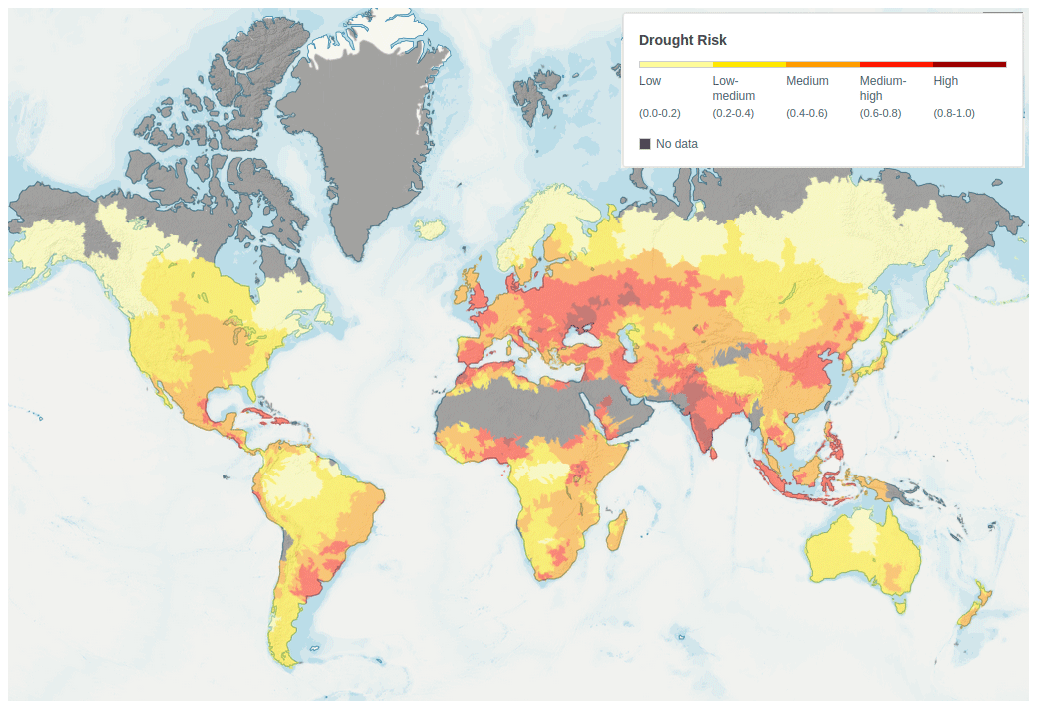
Figure 1Drought risk index score by countries. It combines information on droughts hazard, exposure, and vulnerability. Higher values indicate a higher risk of drought. Source: WRI Aqueduct (https://www.wri.org/aqueduct; last access: 8 August 2022).
Multiyear droughts are rare extreme events, which are related to large-scale atmospheric teleconnections whose dynamics are dictated by chaotic behaviours. An implication of the rare occurrence of multiyear droughts is the limited availability of data to decipher their frequency and train prediction models. For the same reason, it is also difficult to predict how climate change may exacerbate drought risk. Indeed, the warmer climate is changing the hydrological cycle and further affects precipitation (Trenberth, 2011), with evidence demonstrating that precipitation is altering in terms of both annual mean (Knutti and Sedláček, 2013), seasonal variation (Polade et al., 2014; D. Kumar et al., 2014), and extreme events (Papalexiou and Montanari, 2019; Alexander et al., 2006). According to the Intergovernmental Panel on Climate Change Sixth Assessment Report (IPCC AR6), such changing conditions are likely to continue in the 21st century (IPCC, 2021). Therefore, the risk of multiyear droughts is likely to increase in the future, in view also of the increased water demands originated by global warming (Li et al., 2020).
The above reasoning highlights the key role of predictions in mitigating the risk of multiyear droughts and designing adaptation procedures. Future climatic scenarios are usually generated by general circulation models (GCMs), which attempt to simulate future climate variables under given scenarios of CO2 emissions. Recently, the World Climate Research Programme (WCRP) released the Coupled Model Intercomparison Project Phase 6 (CMIP6; Eyring et al., 2016). Simulations from several models are available which deliver ensemble projections of future climate.
The reliability of rainfall simulated by GCMs has been analysed by several studies that focused primarily on the generation of climate models that preceded CMIP6 (CMIP5 and previous models; see Palerme et al., 2017; Koutroulis et al., 2016; Aloysius et al., 2016; S. Kumar et al., 2014; Sillmann et al., 2013). Most of this research compared the climatic scenarios with historical datasets produced by reanalysis such as NCEP or ERA-Interim (Palerme et al., 2017; S. Kumar et al., 2014; Sillmann et al., 2013). However, on the one hand, reanalysis may introduce biases in the reproduction of extreme events. On the other hand, the observation period of these datasets covers only the recent past and therefore may undermine a statistical assessment of performances.
The present study aims at inspecting the ability of selected CMIP6 models in simulating regional-scale climate by focusing on meteorological drought occurrence. We first compare simulated statistics with those of one of the longest daily rainfall records globally available: the Bologna rainfall series, whose observation period dates back to 1813. We decided to adopt an observed record as a baseline instead of a reanalysis to take advantage of an extraordinarily long observation period. Second, we assess meteorological drought changes up to 2100.
The purpose of our study is twofold: (i) to evaluate the ability of up-to-date GCMs in simulating the statistics of observed precipitation by focusing on multiyear meteorological droughts and (ii) to infer how precipitation and drought risk will change in the future. The paper is organized as follows: Sect. 2 provides detailed descriptions of the data used in this study. Sections 3–5 describe the methods for bias correction, reliability testing, and future change assessment. Section 6 presents the results of the historical evaluation and future projections for both precipitation and drought risk. Finally, Sect. 7 summarizes our conclusions.
2.1 Rainfall observations
Italy is one of the first countries that started to systematically collect meteorological observations. Meteorological instruments and a network of observations were developed by Galileo’s scholars and operated in the 17th century already. The rainfall series collected in Padua since 1725 is the longest daily record in the world, and five other rainfall stations have been continuously in operation – with few missing values – since the 18th century (Bologna, Milan, Rome, Palermo, and Turin). Therefore, a data set of enormous value has been accumulated in Italy over the last 3 centuries (Brunetti et al., 2006).
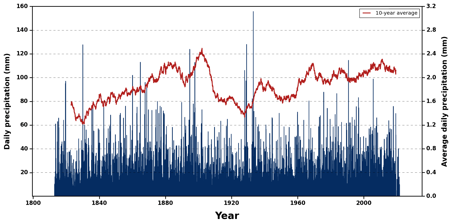
Figure 2Daily rainfall records in Bologna during 1813–2021, with 10-year moving average (red line).
Rainfall observation in Bologna at a daily timescale dates back to 1714. The series in continuous from 1813 onwards. Brunetti et al. (2001) provided an interesting description of the history of the time series. The observatory was originally located in the centre of the city. The rain gauge was changed in 1857 and likely in 1900. After 1978 data were collected by another observatory in a nearby location. Brunetti et al. (2001) proposed monthly correction factors to resolve apparent underestimation of rainfall during 1813–1858, 1900–1928, and 1813–1978. These corrections are valid for monthly rainfall only.
The daily rainfall series observed in Bologna from 1813 to 2021 can be obtained from the European Climate Assessment & Dataset (ECA & D) (https://climexp.knmi.nl/, last access: 9 March 2022). These are original data as reported in the transcripts of the observatory, without any correction. For the purpose of the present analysis, we assume that the daily series is homogeneous. In view of the time window adopted by CMIP6 GCMs for the historical reconstruction, we limit our analysis of the Bologna time series to period of 1850 to 2014 (see Sect. 2.2).
Figure 2 shows the daily time series and the 10-year moving average, which oscillates between a minimum of 1.2 mm and a maximum of 2.5 mm (more than twice the minimum). The above extreme values occurred in the 1820s and the decade ending in 1902, respectively. After 1950, a mild increasing trend is noticed, which mirrors a similar tendency that occurred from the 1830s to the 1890s.
2.2 General circulation model simulation
GCM simulations for both historical (1850–2014) and future (2015–2100) periods are publicly available from the Copernicus database (https://cds.climate.copernicus.eu/, last access: 9 March 2022). Future projections are obtained under the emission scenarios “Shared Socioeconomic Pathway” (SSP) 1-2.6 (SSP1-2.6), 2-4.5 (SSP2-4.5), and 5-8.5 (SSP5-8.5). These are the future emissions considered by the Scenario Model Intercomparison Project (ScenarioMIP) (O'Neill et al., 2016) of CMIP6.
From each model, an ensemble simulation is generated for different initial conditions, initialization methods, physics versions, and forcing datasets. Similarly to Grose et al. (2020) and Kim et al. (2020), we analyse only the first run of each ensemble, which is identified by the abbreviation “r1i1p1f1”, where “r”, “i”, “p”, and “f” indicate initial conditions, initialization method, physics version, and forcing data set, respectively (see https://pcmdi.llnl.gov/CMIP6/Guide/dataUsers.html, last access: 9 March 2022, for more details). We assume that analysing a single ensemble member per GCM is sufficient to sample the ensemble for testing model bias. The assumption above was recently proved to be tenable by Longmate et al. (2023).
Table 1 shows detailed information for 13 GCMs used in this study. We select all the models providing future simulations for the three considered emission scenarios. The multi-model ensemble mean is the arithmetic average value of the 13 GCM outputs.

Simulations by GCM are provided at the grid scale. To compare them with observed data, one should take into account the potential bias that may be introduced by subgrid variability. For the considered timescale subgrid variability is expected to be limited in the region of Bologna. In fact, we focus on monthly and annual rainfall data, which exhibit low spatial variability in the region (see the annual reports of the Regional Agency for Environmental Protection at https://www.arpae.it, last access: 20 February 2023; see also Antolini et al., 2016, for an analysis of subgrid variability in the considered spatial domain).
To compensate for potential bias, we applied bilinear spatial interpolation to estimate the model prediction for Bologna depending on the four nearest GCM grid points. Moreover, we applied quantile delta mapping (QDM) to correct bias with respect to the observed daily rainfall series.
QDM (Cannon et al., 2015) preserves model-projected relative change in quantiles while at the same time correcting the systematic biases in quantiles of a model simulation compared to observed values. It is widely adopted for bias correction of GCM output such as precipitation (Xavier et al., 2022; Fauzi et al., 2020). Here, we apply QDM to the model runs for the historical (1850–2014) and future periods (2015–2100).
First, we compute the empirical frequency of non-exceedance qf(t) of each GCM-simulated value mf(t) during the future (denoted by the subscript “f”) period. Then, the relative change in quantiles Δ(t) of GCM-simulated precipitation over two time periods is given by
where Ff and Fh denote the distribution of empirical frequencies of each GCM-simulated value during the future and historical period, respectively. Then, the bias-corrected value corresponding to qf(t) is computed by the frequency of non-exceedance Fo of the observations during the historical period:
Finally, the bias-corrected GCM simulation for the future period is given by
Note that bias correction for the historical GCM simulation only needs the application of Eq. (2) by plugging in qh(t) in the right-hand side instead of qf(t).
The reliability of GCM simulations with and without bias correction is evaluated by focusing on different temporal scales to obtain a comprehensive picture of model performances.
4.1 Monthly and annual rainfall
To assess the performance of each of the considered CMIP6 GCMs in reproducing the statistics of monthly data during the historical period (1850–2014), we use the “combined probability–probability” (CPP) plot (Koutsoyiannis and Montanari, 2022).
The CPP plot compares the probability distributions Fo and Fh of observed and GCM-simulated monthly rainfall, respectively, during the historical period. The comparison refers to five subsequent 33-year-long time windows during 1850–2014 to assess the capability of GCMs to reproduce changes along the time of climate statistics.
To make the CPP plot, first a realization w from uniform random variable Fw is generated in the range [0, 1], and then we compute the empirical probability distribution:
The ability of GCM in reproducing observed statistics is regarded as good if the plot Fw(w) versus w is the equality line, that is, if Fw(w)=w. This is possible only if Fh is identical to Fo, which is what we would like to check. In essence, the plot tests whether the two distributions, estimated from the GCM simulation and observation, are identical. Note that a CPP plot lying above (below) the equality line indicates underestimation (overestimation) while an S-shaped CPP plot with the initial part above (below) the equality line and the second part below (above) the equality line indicates an underestimation of low (high) rainfall and overestimation of high (low) rainfall (Koutsoyiannis and Montanari, 2022). We also compare the observed and simulated empirical density distributions and lag-1 autocorrelation coefficient of annual rainfall for the whole historical period. Autocorrelation is particularly interesting as it indicates the capability of models to simulate long-term cycles, such as those occurring during multiyear droughts.
4.2 Mean monthly and seasonal rainfall
The goodness of the simulation of monthly and seasonal rainfall averaged over the observation period is evaluated by a graphical comparison with the observed values and the Taylor diagram (Taylor, 2001). The latter is widely applied to summarize how accurately a model simulates an observed record. It integrates three statistical metrics: correlation (R), the centred root-mean-square error (CRMSE), and the ratio of standard deviation (SD) in a single diagram. The angular coordinate represents R. The CRMSE is measured by the distance from the point of reference (observation). Finally, the radial distance from the origin represents the ratio of SD between model simulation and observation. For perfect model simulation, R and the SD ratio assume unit value and CRMSE = 0. These statistics provide a quick summary of the correspondence between the modelled and observed mean monthly and seasonal rainfall, which is particularly useful in assessing the relative merits and overall performance of climate models (Rivera and Arnould, 2020; Dong and Dong, 2021; Yazdandoost et al., 2021). The Taylor diagram is herein used to assess the goodness of the fit of (a) the mean monthly rainfall, (b) March–April–May (MAM) mean rainfall, (c) June–July–August (JJA) mean rainfall, (d) September–October–November (SON) mean rainfall, and (e) December–January–February (DJF) mean rainfall.
4.3 Meteorological droughts
To test the GCM's reliability in simulating multiyear meteorological droughts we apply run theory (Yevjevich, 1967) to annual rainfall to characterize drought events in terms of drought frequency, duration, severity, and intensity. Run theory is one of the most effective approaches for drought identification and has been applied in several areas worldwide (Mishra et al., 2009; Wu et al., 2020; Ho et al., 2021).
In detail, the long-term mean rainfall RLT is adopted as the threshold to identify positive or negative runs (see Fig. 3). If rainfall in a given year is lower than an assigned threshold Tlower<RLT, a negative run is started which ends in the year when the rainfall is higher than RLT. If the interval between two negative runs is only 1 year and rainfall in that year is less than a selected threshold Tupper>RLT, then these two runs are combined into one drought. Finally, only runs which have a duration of no less than 3 years are determined to be multiyear drought events. Here, the thresholds Tupper and Tlower are defined as 20 % more and 10 % less than RLT, respectively. The threshold values have been identified with a trial and error procedure by verifying that relevant droughts observed in the past have been consistently recognized.
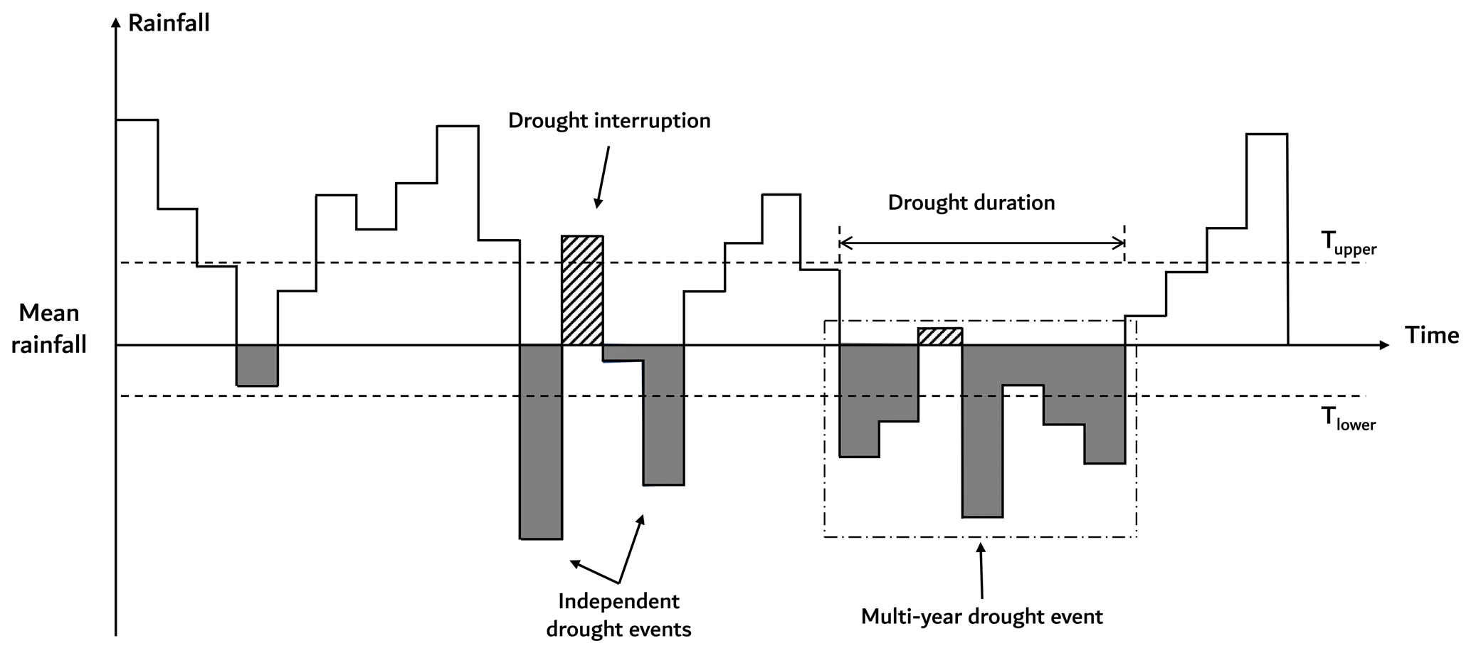
Once a multiyear drought has been identified, drought duration is the time span between the start and the end of the event, and drought severity is computed as the cumulative rainfall deficit with respect to RLT during drought duration divided by the mean rainfall, and drought intensity is computed as the ratio between drought severity and duration. We also estimate the maximum deficit of the drought event, namely, the largest difference between annual rainfall and RLT during the event. Finally, drought frequency is computed as the ratio between the number of drought events that have been identified and the length of the observation period.
Statistics of future projections of annual and seasonal rainfall of the 13 considered GCMs under the three considered scenarios are compared with observed and simulated statistics of the historical period to evaluate future climate change in the Bologna region. For a detailed comparison of seasonal rainfall, the future time horizon is divided into near-future (2030–2059) and far-future (2070–2099) time windows. The multi-model median and the 25th–75th percentiles of the projections given by the GCMs are considered for each scenario to represent the associated ensemble uncertainty.
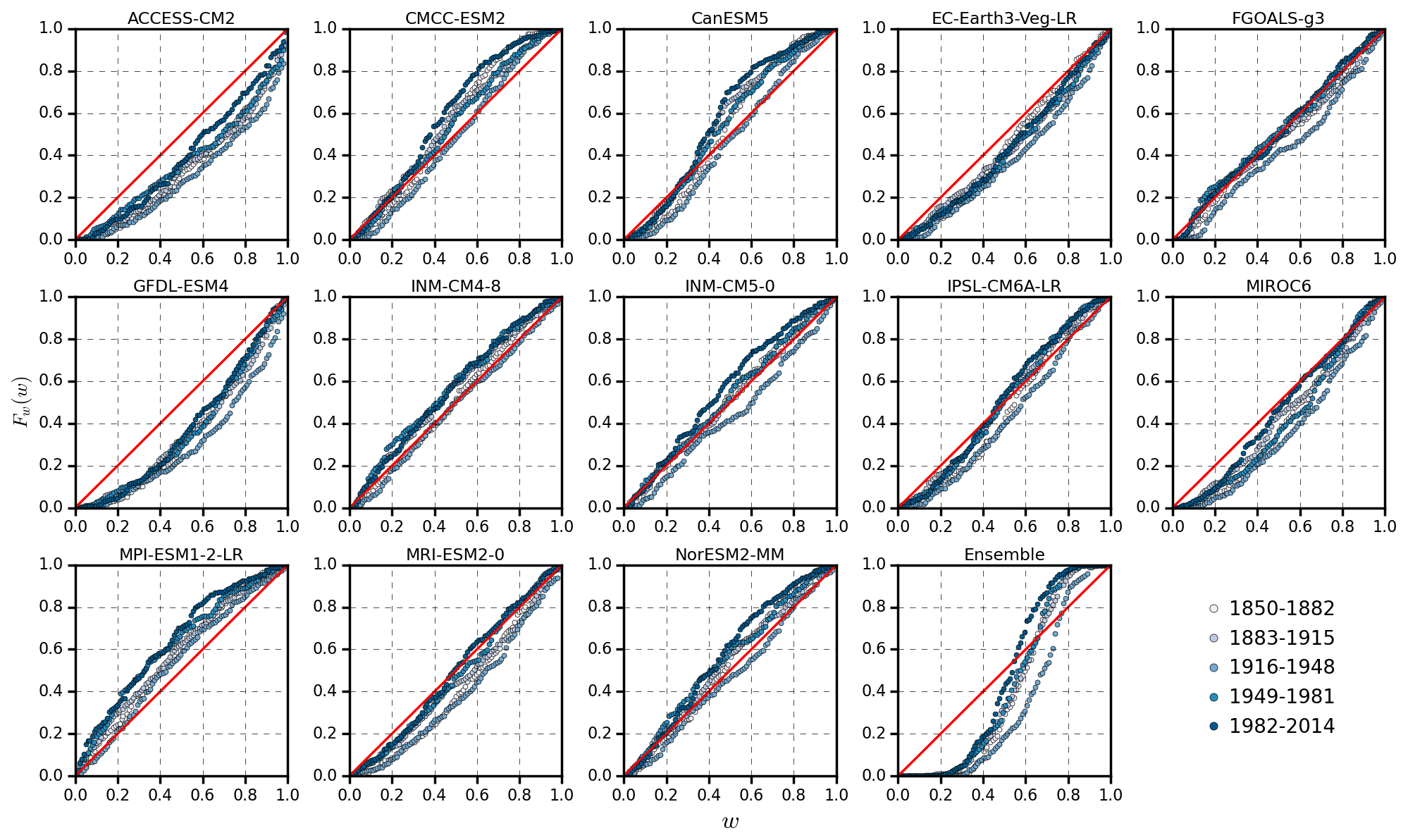
Figure 4Combined probability–probability plot of observed and GCM-simulated monthly rainfall in five time windows during the historical period before bias correction.
6.1 Reliability of historical data simulation
6.1.1 Monthly and annual rainfall
Figures 4 and 5 show the CPP plots of observed and simulated monthly rainfall time series in the five subsequent time windows during the historical period before and after QDM bias correction, respectively. Note that QDM was operated over the whole historical period.
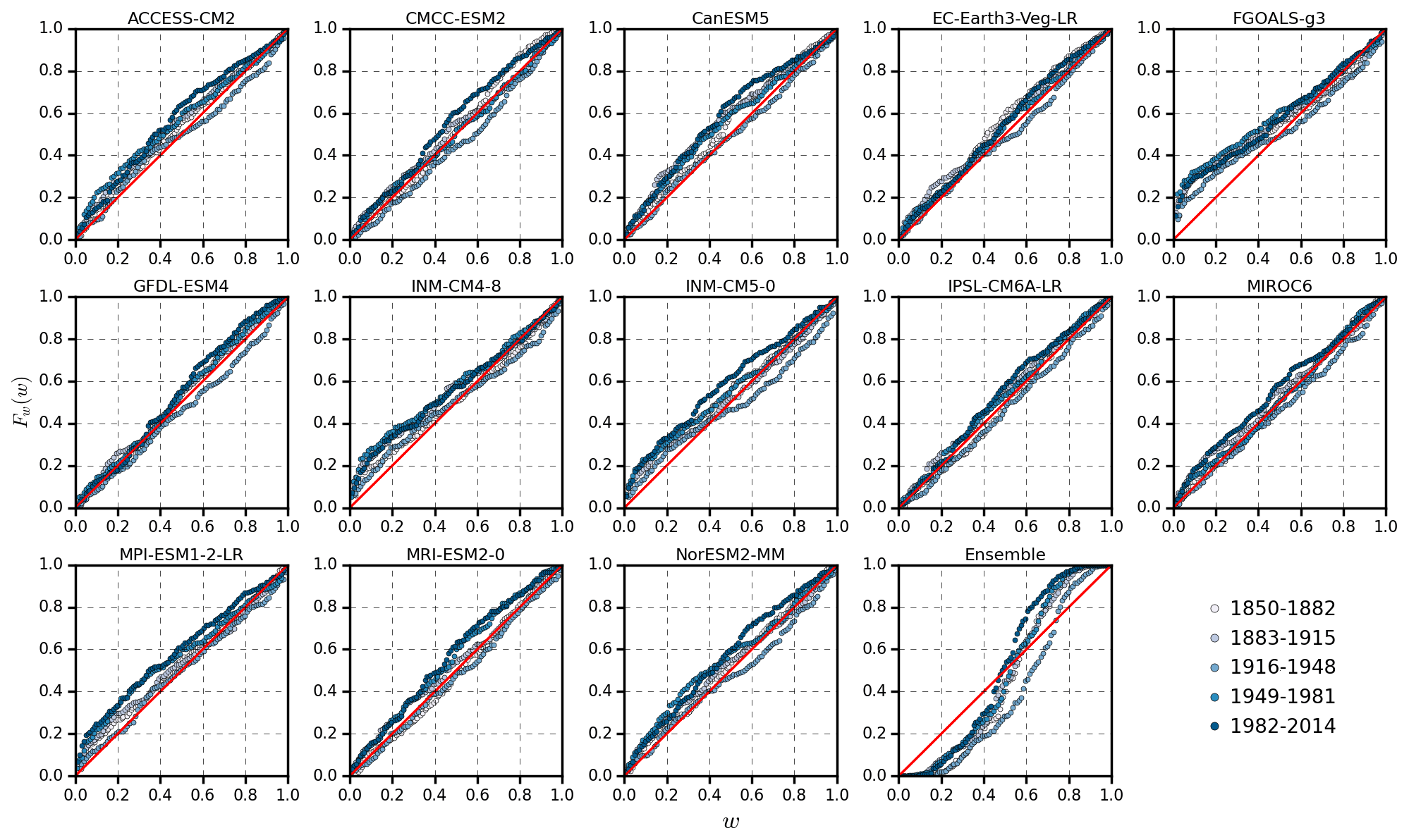
Figure 5Combined probability–probability plot of observed and GCM-simulated monthly rainfall in five time windows during the historical period after bias correction.
While each individual model displays consistent performance in terms of probability distribution across various time windows with only minor differences, the results do not allow easy identification of the optimal model for a given time window. Before bias correction, MPI-ESM1-2-LR generally underestimates monthly rainfall for all periods while some other models (ACCESS-CM2, GFDL-ESM4, and MIROC6) end up with a prevailing overestimation. CMCC-ESM2 and CanESM5 relatively well capture the low rainfall, while underestimating high rainfall. The remaining models (e.g. FGOALS-g3, IPSL-CM6A-LR, and INM-CM4-8) generally fit the observed distribution well in some time windows while exhibiting slight departures in other periods. The multi-model ensemble satisfactorily simulates the mean value while overestimating and underestimating the low and high rainfall, respectively.
As expected, after bias correction all models show a better performance in reproducing probability distributions in different periods except FGOALS-g3 and INM-CM4-8, which slightly underestimate low rainfall after QDM. The performance of the ensemble remains somewhat consistent, although for some periods one notes an improvement in the fit of the mean value. In general, it is confirmed that bias correction improves the model performances for historical simulations. The obvious limit of QDM is the requirement of an extended data set of historical data.
For the whole historical period, Fig. 6 shows a comparison between observed and simulated empirical density distribution of annual rainfall before and after bias correction. Before QDM, the majority of models perform worse in capturing heavier rainfall than lighter rainfall, with the opposite result occurring for EC-Earth3-Veg-LR, MIROC6, and MRI-ESM2-0. Only ACCESS-CM2 and GFDL-ESM4 overestimate both high and low rainfall. After QDM, all the models exhibit improved performances although underestimation of high rainfall is introduced by QDM for seven models and the ensemble simulation. It is noted that multi-model ensemble (MME) mean exhibits lower variability with respect to observed data both before and after bias correction. This result is coherent with what is shown in Figs. 4 and 5.
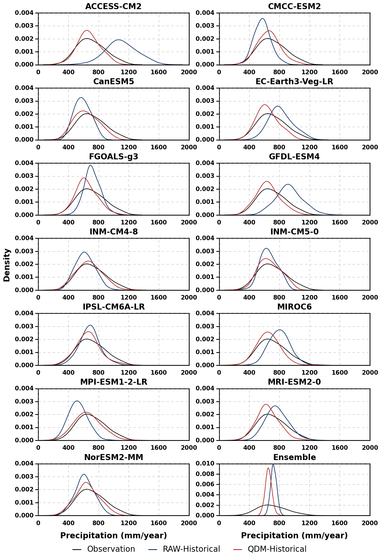
Figure 6Comparison of sample probability density of annual rainfall for observations and GCM historical simulations.
Table 2 displays the lag-1 autocorrelation coefficient for each model simulation before and after QDM bias correction. It is interesting to note that the correlation of observed data is slightly higher in than all the models, therefore highlighting a possible model weakness in simulating temporal correlation. Since the coefficient of the observation series is 0.226, the observed values may be correlated in pairs or triplets while most of the GCMs' series are uncorrelated, thereby implying a possible inadequacy of bi-annual or triennial fitness. After QDM, the correlation decreases which indicates that QDM may influence the autocorrelation of the raw output of GCM.
Table 2Lag-1 autocorrelation coefficient between observed annual rainfall and each historical simulation before and after bias correction.
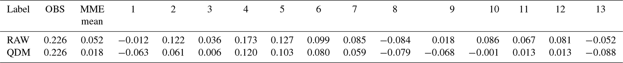
OBS is observation data, MME mean is multi-model ensemble mean, and numbers indicate models: 1 – ACCESS-CM2; 2 – CMCC-ESM2; 3 – CanESM5; 4 – EC-Earth3-Veg-LR; 5 – FGOALS-g3; 6 – GFDL-ESM4; 7 – INM-CM4-8; 8 – INM-CM5-0; 9 – IPSL-CM6A-LR; 10 – MIROC6; 11 – MPI-ESM1-2-LR; 12 – MRI-ESM2-0; 13 – NorESM2-MM.
6.1.2 Mean monthly and seasonal rainfall
Figure 7 shows the graphical comparison between observed and simulated mean monthly rainfall for the whole historical period before bias correction. Most of the models adequately replicate the seasonal rainfall pattern except INM-CM4-8 and FGOALS-g3. However, ACCESS-CM2 overestimates rainfall for all months. Moreover, all models except MPI-ESM1-2-LR, CMCC-ESM2, NorESM2-MM, and CanESM5 overestimate rainfall in DJF. Conversely, all models except ACCESS-CM2, GFDL-ESM4, EC-Earth3-Veg-LR, and MRI-ESM2-0 underestimate JJA and/or SON rainfall. For MAM rainfall, several models exhibit overestimation. In addition, the MME mean satisfactorily reproduces the annual cycle of rainfall, especially MAM rainfall while slightly underestimating JJA and SON and overestimating DJF rainfall.
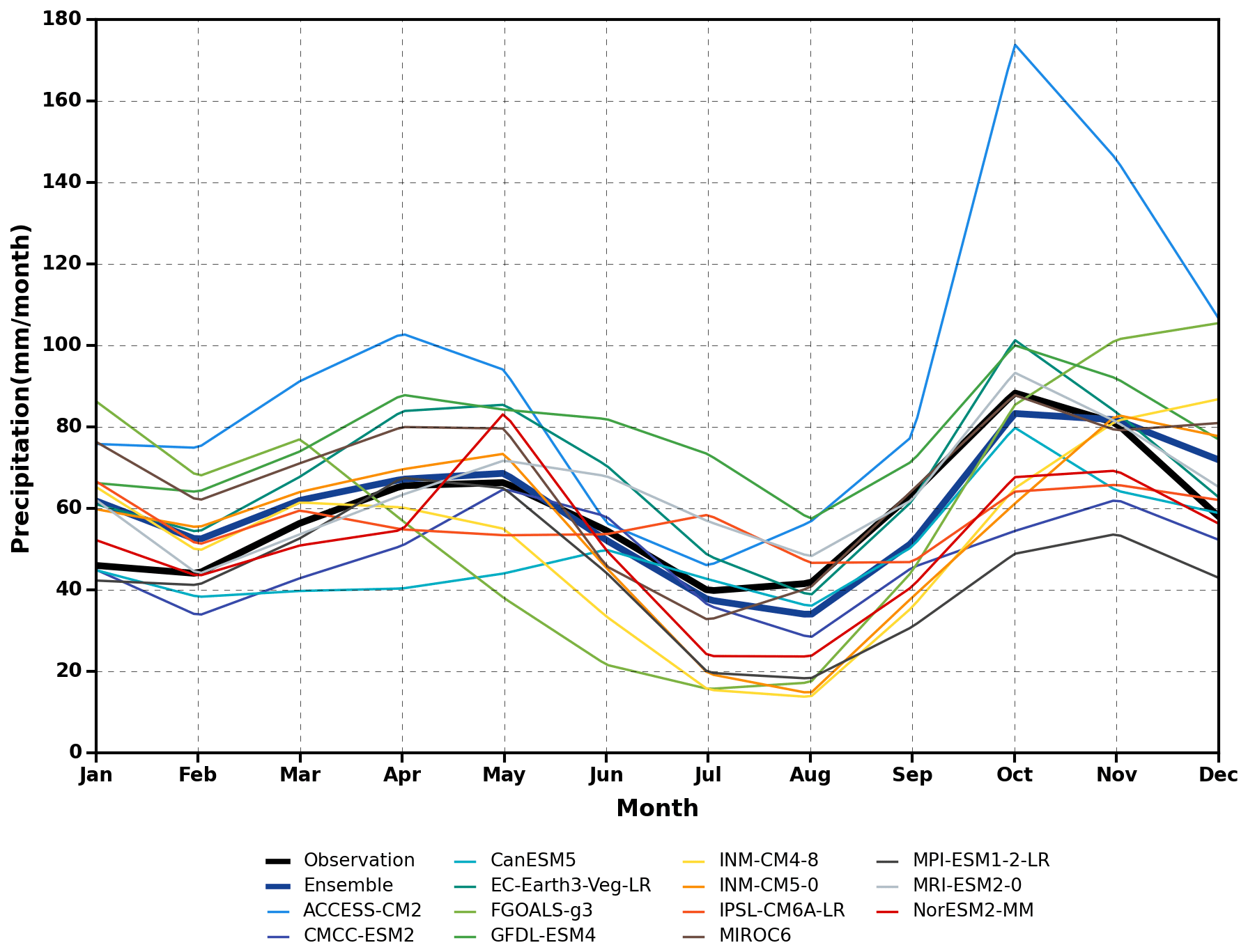
Figure 7Annual cycle of historical (1850–2014) mean monthly rainfall (mm per month) of the MME mean and CMIP6 models against observation data.
Figure 8 displays the same graphical comparison after QDM. Although INM-CM4-8 and FGOALS-g3 still fail to reproduce the seasonal pattern, the performance of ACCESS-CM2 has been improved. Other models show improvement in some seasons only (e.g. NorESM2-MM better captures SON rainfall but shows worse performances for MAM rainfall). In general, most of the models underestimate summer JJA rainfall after QDM.
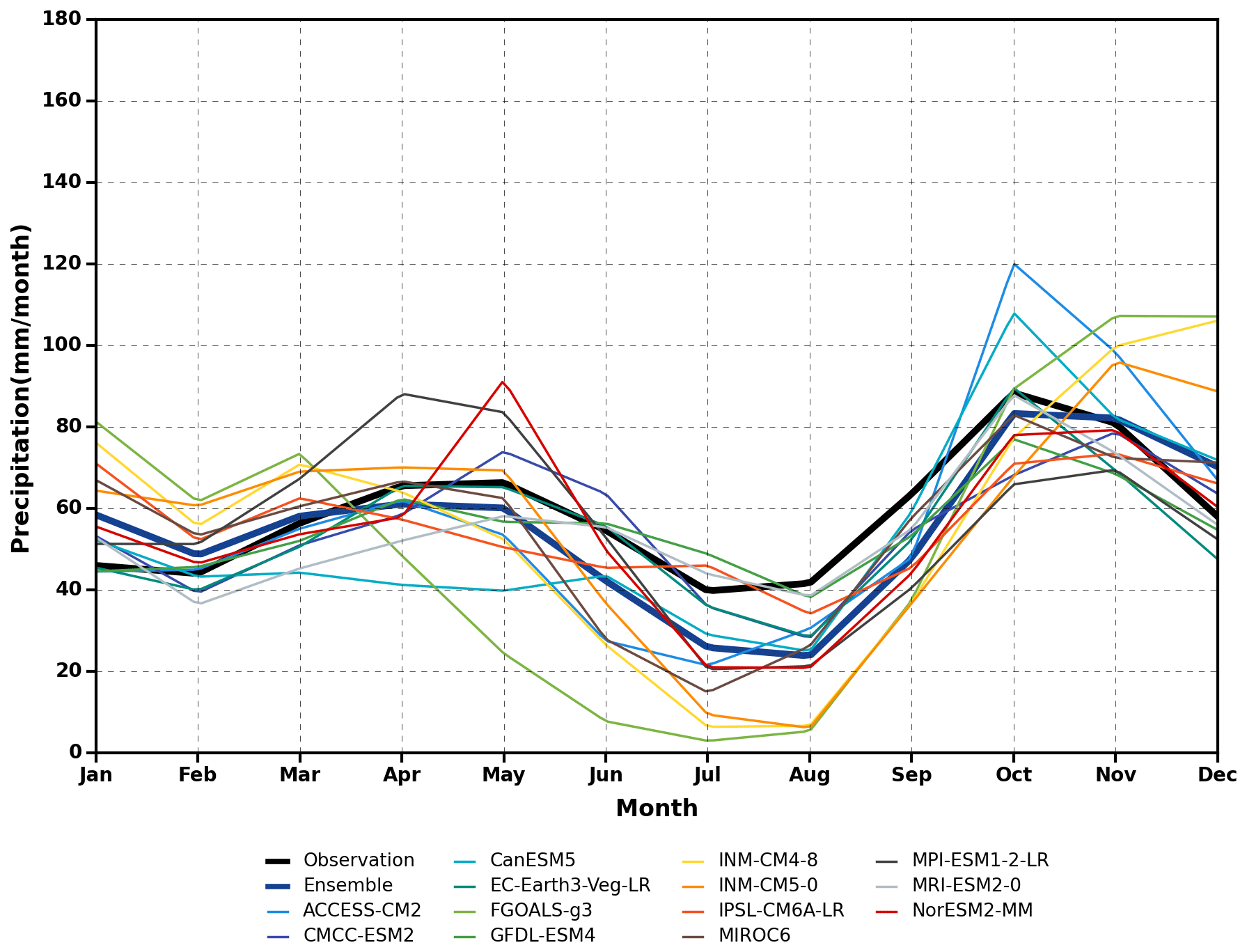
Figure 8Annual cycle of historical (1850–2014) mean monthly rainfall (mm per month) of the MME mean and CMIP6 models against observation data after bias correction.
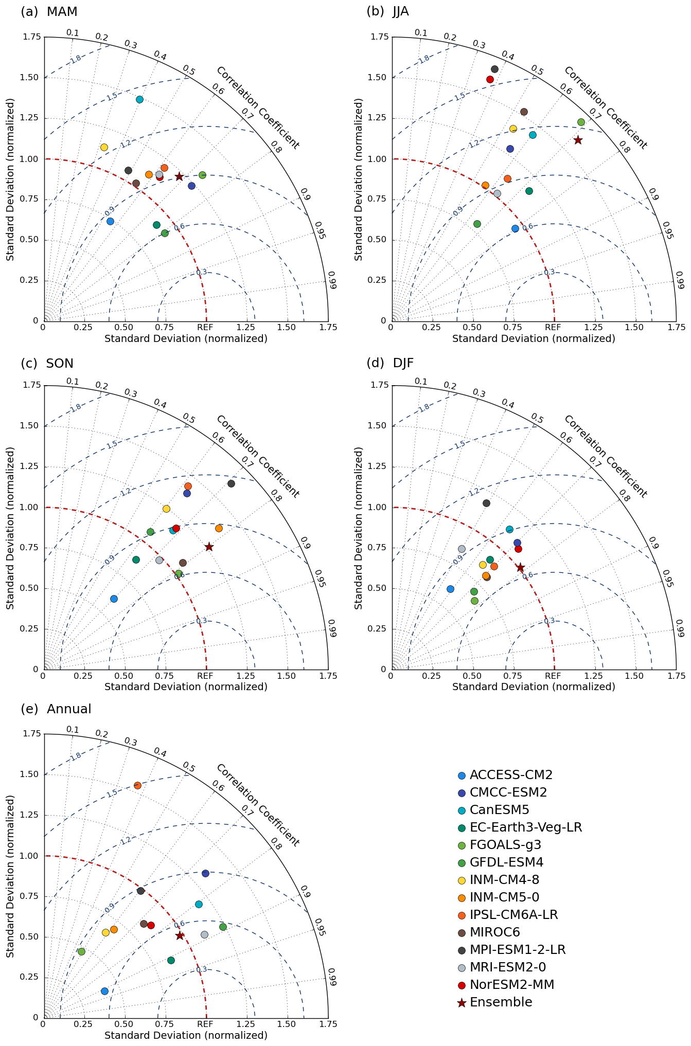
Figure 9Taylor diagram of (a) March–April–May (MAM), (b) June–July–August (JJA), (c) September–October–November (SON), (d) December–January–February (DJF), and (e) annual cycle of historical (1850–2014) mean monthly rainfall for the GCMs and their MME mean before bias correction.
Figure 9 shows the Taylor diagram for each GCM and the MME mean when simulating the seasonal rainfall pattern. It confirms that six of the models and the MME mean adequately replicate the mean monthly rainfall with relatively high R, low CRMSE, and low SD. In particular, satisfactory results are provided by EC-Earth3-Veg-LR and MRI-ESM2-0. IPSL-CM6A-LR and FGOALS-g3 display relatively poor performance. However, a considerable improvement is exhibited in reproducing MAM, SON, and DJF rainfall for these two models, especially FGOALS-g3, which can simulate SON rainfall best. For DJF rainfall, all models show a better performance with respect to other seasons, and the MME mean shows the best performance of any individual model. Most of the models depict a worse performance in SON and JJA than MAM and DJF with much larger bias. In general, the EC-Earth3-Veg-LR provides a satisfactory simulation of both annual cycle and each seasonal rainfall, while GFDL-ESM4, ACCESS-CM2, and FGOALS-g3 can better reproduce the MAM, JJA, and SON rainfall, respectively. Although R is slightly lower than the EC-Earth3-Veg-LR, the MME mean performs satisfactorily in simulating the annual cycle of rainfall and best captures DJF rainfall but shows no advance over the single models in reproducing MAM, JJA, and SON rainfall.
Figure 10 shows the Taylor diagram after QDM. In general, several models show higher CRMSE for JJA rainfall and lower SD for SON rainfall, while the performance for MAM rainfall is similar before and after QDM. Although QDM displays no evident improvement in the models' ability to capture seasonal rainfall patterns, one notes a slightly enhanced performance for the SON season. Overall, the models still show a better ability to reproduce DJF rainfall compared to other seasons. For the annual cycle, individual models (e.g. GFDL-ESM4 and MRI-ESM2-0), exhibit improved simulation abilities, but the MME mean shows a higher SD after bias correction.
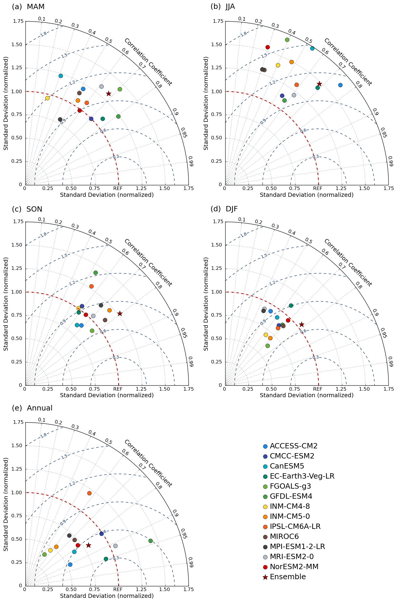
Figure 10Taylor diagram of (a) March–April–May (MAM), (b) June–July–August (JJA), (c) September–October–November (SON), (d) December–January–February (DJF), and (e) annual cycle of historical (1850–2014) mean monthly rainfall for the GCMs and their MME mean after bias correction.
6.1.3 Meteorological droughts
Tables 3 and 4 show the characteristics of multiyear droughts derived by using run theory for both observations and each model simulation before and after bias correction for both the whole historical and whole future periods, the latter for SSP2.6 and SSP8.5 scenarios. For the observation data, the long-term mean value of annual rainfall, which has an RLT of 705 (mm yr−1), is regarded as the threshold to identify the observed multiyear drought events.
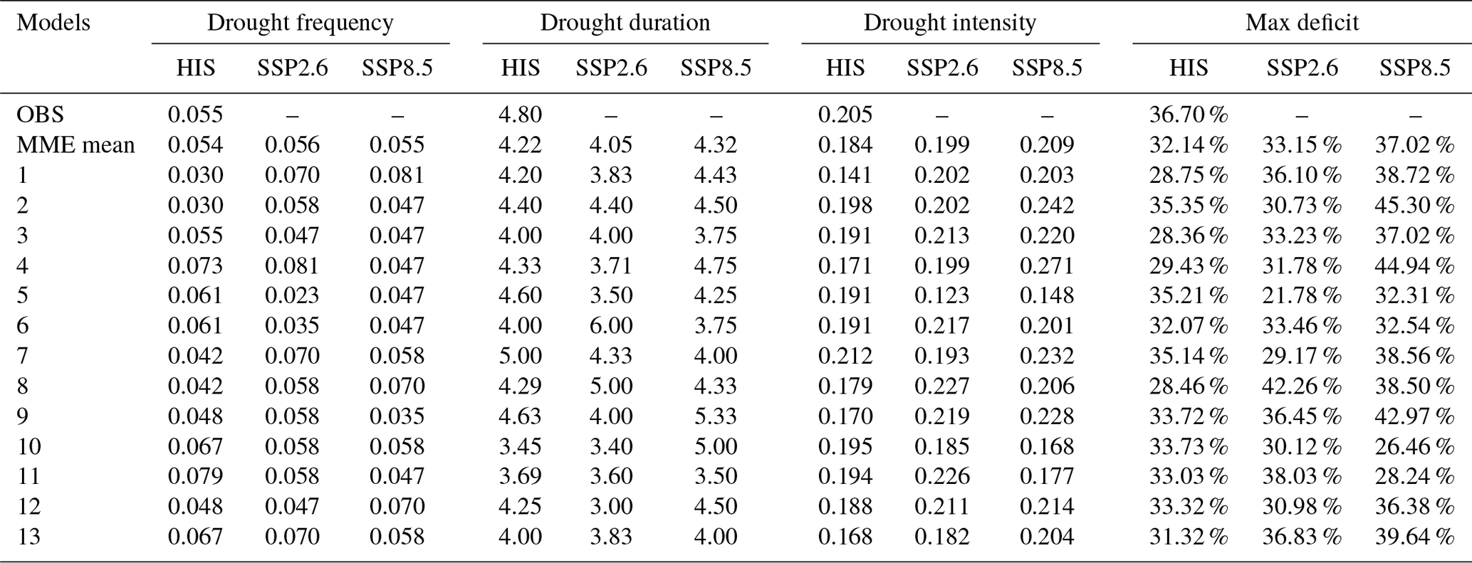
Table 3Mean values over the considered period of drought frequency (DF), duration (DD), intensity (DI), and maximum deficit (MD) for multiyear meteorological droughts exhibited by observed data (1850–2014) and reproduced by models before bias correction for the historical (1850–2014) and future (2015–2100) periods under the two considered scenarios.
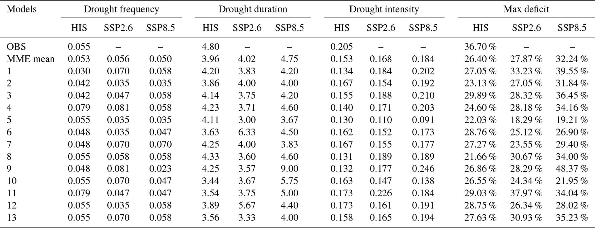
The unit of drought frequency is times per year and the unit of drought duration is years. OBS and HIS are observed data and historical simulation. MME mean is multi-model ensemble mean, and different numbers indicate different models: 1 – ACCESS-CM2; 2 – CMCC-ESM2; 3 – CanESM5; 4 – EC-Earth3-Veg-LR; 5 – FGOALS-g3; 6 – GFDL-ESM4; 7 – INM-CM4-8; 8 – INM-CM5-0; 9 – IPSL-CM6A-LR; 10 – MIROC6; 11 – MPI-ESM1-2-LR; 12 – MRI-ESM2-0; 13 – NorESM2-MM.
Table 4Mean values over the considered period of drought frequency (DF), duration (DD), intensity (DI), and maximum deficit (MD) for multiyear meteorological droughts exhibited by observed data (1850–2014) and reproduced by models after bias correction for the historical (1850–2014) and future (2015–2100) periods under the two considered scenarios.
The unit of drought frequency is times per year and the unit of drought duration is years. OBS and HIS are observed data and historical simulation. MME mean is multi-model ensemble mean, and different numbers indicate different models: 1 – ACCESS-CM2; 2 – CMCC-ESM2; 3 – CanESM5; 4 – EC-Earth3-Veg-LR; 5 – FGOALS-g3; 6 – GFDL-ESM4; 7 – INM-CM4-8; 8 – INM-CM5-0; 9 – IPSL-CM6A-LR; 10 – MIROC6; 11 – MPI-ESM1-2-LR; 12 – MRI-ESM2-0; 13 – NorESM2-MM.
The results highlight that FGOALS-g3, INM-CM5-0, MIROC6, MPI-ESM2-0, and NorESM2-MM simulate drought frequency (DF) fairly well. Notably, all models fail to replicate the drought duration (DD), drought intensity (DI), and maximum deficit (MD). For instance, IPSL-CM6A-LR and INM-CM4-8 show the best performance in simulating DD, which, however, is underestimated by about 10 % by the best simulation. Although MPI-ESM1-2-LR presents the highest value of DI and MD against all the models, marked underestimation with respect to the observations still occurs. The MME mean displays relatively good performance in terms of DF but still underestimates DD, DI, and MD. In detail, the MME mean DD is underestimated by about 17 %, while DI and MD for observations are even nearly 34 % and 39 % higher than the MME mean, respectively.
After QDM, a slight improvement is obtained for the simulation of DF. The MME mean confirms its satisfactory performance, although six models still end up with underestimation. Notably, all models still fail to replicate the DD, DI, and MD, with the only exception being INM-CM4-8, which satisfactorily reproduces drought characteristics. In general, the impact of QDM varies depending on each model and drought behaviour.
QDM slightly mitigates the underestimation by the MME mean of DD, DI, and MD, which, however, remain 12 %, 10 %, and 12 % lower than observations, respectively.
6.2 Future changes
6.2.1 Changes in average rainfall
Figure 11 shows the future projections of annual rainfall after QDM for three different scenarios (SSP1-2.6, SSP2-4.5, and SSP5-8.5), compared with the MME mean simulation of the historical period (1850–2014). Future annual rainfall shows only a slight decrease for the SSP5-8.5 scenario while fluctuating with close to stationary behaviour with respect to the historical period. After applying bias correction, future projections exhibit similarities to the raw output but with a slightly lesser degree of change.
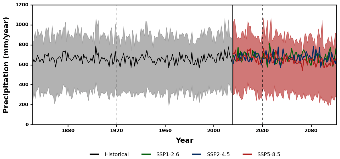
Figure 11Time series of annual rainfall for both the historical simulation and future projections after bias correction (mm yr−1). Historical simulation (black) and future MME mean simulations for SSP1-2.6 (green), SSP2-4.5 (blue), and SSP5-8.5 (red). The uncertainty ranges for the historical simulation (grey shading) and future projection under SSP5-8.5 (red shading) are shown in the 25th and 75th percentiles of the ensemble.
To inspect the temporal progress of changes, the annual cycle of rainfall after bias correction is considered and the future period is divided into the near future (2030–2059) and far future (2070–2099) related to the present-day simulation (1985–2014). Figure 12 shows an overall decrease in monthly rainfall under all the scenarios in each future period. Under the SSP2.6 scenario, the MAM rainfall in the far future is expected to be less than in the near-future period. Conversely, the rainfall during the SON season in the far future will be higher than in the near future. Moreover, rainfall may be more likely to be concentrated in November rather than in October in both periods. This change in rainfall pattern also occurs in the near-future period under the SSP4.5 scenario, but the overall monthly rainfall shows no evident difference between periods. Under the SSP8.5 scenario, the MAM and JJA rainfall in the far future will be considerably less than in the near future, and the rainfall will be more concentrated in the SON and DJF season. The results after QDM depict an analogous future change in the seasonal rainfall pattern. With respect to raw output, however, the JJA season is projected to be drier after QDM, which aligns with the historical simulation.
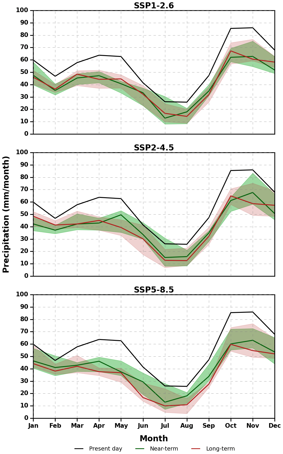
Figure 12Monthly mean rainfall (mm per month) for multiple models in the present day (1985–2014), near future (2030–2059), and far future (2070–2099) under SSP1-2.6, SSP2-4.5, and SSP5-8.5 scenarios. Thick lines indicate multi-model medians, while shading indicates the 25th–75th percentile model ranges.
6.2.2 Future meteorological drought changes
Table 3 reports future drought changes for SSP2.6 and SSP8.5 future scenarios. Corresponding statistics for observed data (whole 1850–2014 observations) and model simulations for the historical period (1850–2014) are also shown.
The future changes in DF with respect to historical simulations are not remarkable. DD, DF, and MD are generally underestimated with respect to historical data. In fact, the values of DD, DI, and MD for the MME mean under SSP2.6 and SSP8.5 are both lower with respect to observations. Moreover, DD of all models except GFDL-ESM4 is shorter under SSP2.6 with respect to observed data. Only the MME mean and models CMCC-ESM2, MIROC6, and MPI-ESM1-2 show a consistent increase in DD when turning from the historical simulation to SSP2.6 and SSP8.5. Nearly all models show an increase in DI with respect to historical simulations for at least one future scenario, and all models except FGOALS-g3 and MIROC6 show a more intense drought under SSP8.5 than SSP2.6. Changes in MD are similar to DI. The above considerations show that historical data depict a worse future in terms of multiyear droughts with respect to simulations before QDM.
Table 4 presents the corresponding future drought changes after QDM. The good performance of the MME mean in terms of DF is confirmed. However, more models exhibit less DF compared to observations under SSP8.5. For DD, QDM results in a general deterioration of performances in terms of underestimation. For DI and MD, similar values to observed data are reached by the MME mean under SSP8.5 only but with large variability among models. In general, QDM improves MME mean performances, but one still notes large variability among models. Moreover, the expectation of increased drought risk in the future with respect to historical observations is not confirmed even after QDM and the application of the worst emission scenario.
The present study refers to the region of Bologna, where the availability of a 209-year-long daily rainfall series allows us to make a unique assessment of GCMs' reliability and their predicted changes in rainfall and drought risk. The results show that GCMs provide a satisfactory simulation of rainfall seasonality, while statistics of rainfall series estimated for the long-term historical period exhibit discrepancies among models and limited reliability in some cases. In particular, the GCMs show weakness in capturing the correlation of annual rainfall, thereby implying a possible lack of fit in the simulation of cycles.
In fact, our focus is concentrated on the statistics of multiyear droughts. We found that the multi-model ensemble can satisfactorily simulate the mean frequency of droughts during the historical period. Conversely, the mean duration, intensity, and maximum deficit of multiyear droughts are underestimated.
Bias correction with QDM improves the simulation of the statistics of the monthly and annual series, while it does not show consistent enhancements in capturing the correlation of annual rainfall and the distribution of seasonal rainfall. The improvement by QDM to simulate drought characteristics is limited. Indeed, future projections by the multi-model ensemble of multiyear droughts depict a similar risk to historical observations, even after bias correction and adopting the most critical emission scenario.
Our results suggest that validation at the local scale of GCM simulations is an essential step to inform downscaling procedures and correction techniques to make sure that model predictions are consistent with the local features of climate. However, extreme events like multiyear droughts are infrequent, and therefore validating their predicted statistics is particularly challenging.
Therefore, the identification of future drought risk, which one would expect to be increased under climate change, remains a challenge, especially if we consider that the reliability of bias correction depends on the availability of observed historical data. For some situations, classical engineering methods for critical event estimation under the assumption of stationarity, with appropriate integration of the information provided by climate models to account for climate change, may still be the most precautionary approach. Therefore, rigorous use and comprehensive interpretation of the available information are needed to avoid mismanagement by also taking into account that the impact of multiyear meteorological droughts is likely to be exacerbated by further pressure on water resources due to increasing population and water demand.
The historical rainfall series observed in Bologna can be obtained from https://climexp.knmi.nl/ (KNMI and WMO, 2022). All the CMIP6 GCM outputs are publicly available from the Copernicus Data Store (https://cds.climate.copernicus.eu/, Copernicus Climate Change Service, 2022).
AM proposed the main research question and supervised the work. RG made the computational analysis, elaborated additional research ideas, and prepared the paper.
The contact author has declared that neither of the authors has any competing interests.
Publisher's note: Copernicus Publications remains neutral with regard to jurisdictional claims in published maps and institutional affiliations.
We thank Zhiqi Yang and Zhanwei Liu for the helpful discussions. We also thank four anonymous reviewers and the editor for their insightful reviews.
Rui Guo was supported by the China Scholarship Council (CSC) Scholarship, no. 202106060061. Alberto Montanari received partial funding from the RETURN Extended Partnership, financed by the National Recovery and Resilience Plan – NRRP, Mission 4, Component 2, Investment 1.3 – D.D. 1243 2/8/2022, PE0000005.
This paper was edited by Lelys Bravo de Guenni and reviewed by four anonymous referees.
Alexander, L. V., Zhang, X., Peterson, T. C., Caesar, J., Gleason, B., Klein Tank, A. M. G., Haylock, M., Collins, D., Trewin, B., Rahimzadeh, F., Tagipour, A., Rupa Kumar, K., Revadekar, J., Griffiths, G., Vincent, L., Stephenson, D. B., Burn, J., Aguilar, E., Brunet, M., Taylor, M., New, M., Zhai, P., Rusticucci, M., and Vazquez-Aguirre, J. L.: Global Observed Changes in Daily Climate Extremes of Temperature and Precipitation, J. Geophys. Res.-Atmos., 111, D05109, https://doi.org/10.1029/2005JD006290, 2006. a
Aloysius, N. R., Sheffield, J., Saiers, J. E., Li, H., and Wood, E. F.: Evaluation of Historical and Future Simulations of Precipitation and Temperature in Central Africa from CMIP5 Climate Models, J. Geophys. Res.-Atmos., 121, 130–152, https://doi.org/10.1002/2015JD023656, 2016. a
Antolini, G., Auteri, L., Pavan, V., Tomei, F., Tomozeiu, R., and Marletto, V.: A daily high-resolution gridded climatic data set for Emilia-Romagna, Italy, during 1961–2010, Int. J. Climatol., 36, 1970–1986, 2016. a
Brunetti, M., Buffoni, L., Lo Vecchio, G., Maugeri, M., and Nanni, T.: Tre Secoli Di Meteorologia a Bologna, Cooperativa Universitaria Studio e Lavoro Milan Rep. 325, 2001. a, b
Brunetti, M., Maugeri, M., Monti, F., and Nanni, T.: Temperature and Precipitation Variability in Italy in the Last Two Centuries from Homogenised Instrumental Time Series, Int. J. Climatol., 26, 345–381, https://doi.org/10.1002/joc.1251, 2006. a
Cannon, A. J., Sobie, S. R., and Murdock, T. Q.: Bias Correction of GCM Precipitation by Quantile Mapping: How Well Do Methods Preserve Changes in Quantiles and Extremes?, J. Climate, 28, 6938–6959, https://doi.org/10.1175/JCLI-D-14-00754.1, 2015. a
Cook, B. I., Cook, E. R., Smerdon, J. E., Seager, R., Williams, A. P., Coats, S., Stahle, D. W., and Díaz, J. V.: North American Megadroughts in the Common Era: Reconstructions and Simulations, WIREs Clim. Change, 7, 411–432, https://doi.org/10.1002/wcc.394, 2016. a, b
Copernicus Climate Change Service – C3S: Climate Data Store (CDS), https://cds.climate.copernicus.eu/ (last access: 9 March 2022), 2022. a
Dong, T. and Dong, W.: Evaluation of Extreme Precipitation over Asia in CMIP6 Models, Clim. Dynam., 57, 1751–1769, https://doi.org/10.1007/s00382-021-05773-1, 2021. a
Eyring, V., Bony, S., Meehl, G. A., Senior, C. A., Stevens, B., Stouffer, R. J., and Taylor, K. E.: Overview of the Coupled Model Intercomparison Project Phase 6 (CMIP6) Experimental Design and Organization, Geosci. Model Dev., 9, 1937–1958, https://doi.org/10.5194/gmd-9-1937-2016, 2016. a
Fauzi, F., Kuswanto, H., and Atok, R.: Bias correction and statistical downscaling of earth system models using quantile delta mapping (QDM) and bias correction constructed analogues with quantile mapping reordering (BCCAQ), J. Phys.: Conf. Ser., 1538, 012050, https://doi.org/10.1088/1742-6596/1538/1/012050, 2020. a
Grose, M. R., Narsey, S., Delage, F. P., Dowdy, A. J., Bador, M., Boschat, G., Chung, C., Kajtar, J. B., Rauniyar, S., Freund, M. B., Lyu, K., Rashid, H., Zhang, X., Wales, S., Trenham, C., Holbrook, N. J., Cowan, T., Alexander, L., Arblaster, J. M., and Power, S.: Insights From CMIP6 for Australia's Future Climate, Earth's Future, 8, e2019EF001469, https://doi.org/10.1029/2019EF001469, 2020. a
Ho, S., Tian, L., Disse, M., and Tuo, Y.: A New Approach to Quantify Propagation Time from Meteorological to Hydrological Drought, J. Hydrol., 603, 127056, https://doi.org/10.1016/j.jhydrol.2021.127056, 2021. a
IPCC: Summary for Policymakers, in: Climate Change 2021: The Physical Science Basis, Contribution of Working Group I to the Sixth Assessment Report of the Intergovernmental Panel on Climate Change, edited by: Masson-Delmotte, V., Zhai, P., Pirani, A., Connors, S., Péan, C., Berger, S., Caud, N., Chen, Y., Goldfarb, L., Gomis, M., Huang, M., Leitzell, K., Lonnoy, E., Matthews, J., Maycock, T., Waterfield, T., Yelekçi, O., Yu, R., and Zhou, B., Cambridge University Press, Cambridge, UK and New York, NY, USA, 3–32, https://doi.org/10.1017/9781009157896.001, 2021. a
Kim, Y.-H., Min, S.-K., Zhang, X., Sillmann, J., and Sandstad, M.: Evaluation of the CMIP6 Multi-Model Ensemble for Climate Extreme Indices, Weather Clim. Extrem., 29, 100269, https://doi.org/10.1016/j.wace.2020.100269, 2020. a
KNMI and WMO – World Meteorological organization: The KNMI climate explorer, https://climexp.knmi.nl/ (last access: 9 March 2022), 2022. a
Knutti, R. and Sedláček, J.: Robustness and Uncertainties in the New CMIP5 Climate Model Projections, Nat. Clim. Change, 3, 369–373, https://doi.org/10.1038/nclimate1716, 2013. a
Koutroulis, A. G., Grillakis, M. G., Tsanis, I. K., and Papadimitriou, L.: Evaluation of Precipitation and Temperature Simulation Performance of the CMIP3 and CMIP5 Historical Experiments, Clim. Dynam., 47, 1881–1898, https://doi.org/10.1007/s00382-015-2938-x, 2016. a
Koutsoyiannis, D. and Montanari, A.: Bluecat: A Local Uncertainty Estimator for Deterministic Simulations and Predictions, Water Resour. Res., 58, e2021WR031215, https://doi.org/10.1029/2021WR031215, 2022. a, b
Kumar, D., Kodra, E., and Ganguly, A. R.: Regional and Seasonal Intercomparison of CMIP3 and CMIP5 Climate Model Ensembles for Temperature and Precipitation, Clim. Dynam., 43, 2491–2518, https://doi.org/10.1007/s00382-014-2070-3, 2014. a
Kumar, S., Lawrence, D. M., Dirmeyer, P. A., and Sheffield, J.: Less Reliable Water Availability in the 21st Century Climate Projections, Earth's Future, 2, 152–160, https://doi.org/10.1002/2013EF000159, 2014. a, b
Li, Z., Fang, G., Chen, Y., Duan, W., and Mukanov, Y.: Agricultural Water Demands in Central Asia under 1.5 ∘C and 2.0 ∘C Global Warming, Agr. Water Manage., 231, 106020, https://doi.org/10.1016/j.agwat.2020.106020, 2020. a
Longmate, J. M., Risser, M. D., and Feldman, D. R.: Prioritizing the selection of CMIP6 model ensemble members for downscaling projections of CONUS temperature and precipitation, Clim. Dynam., https://doi.org/10.21203/rs.3.rs-1428854/v1, in press, 2023. a
Lund, J., Medellin-Azuara, J., Durand, J., and Stone, K.: Lessons from California's 2012–2016 Drought, J. Water Resour. Plan. Manage., 144, 04018067, https://doi.org/10.1061/(ASCE)WR.1943-5452.0000984, 2018. a
Mishra, A. K., Singh, V. P., and Desai, V. R.: Drought Characterization: A Probabilistic Approach, Stoch. Environ. Res. Risk A, 23, 41–55, https://doi.org/10.1007/s00477-007-0194-2, 2009. a
O'Neill, B. C., Tebaldi, C., van Vuuren, D. P., Eyring, V., Friedlingstein, P., Hurtt, G., Knutti, R., Kriegler, E., Lamarque, J.-F., Lowe, J., Meehl, G. A., Moss, R., Riahi, K., and Sanderson, B. M.: The Scenario Model Intercomparison Project (ScenarioMIP) for CMIP6, Geosci. Model Dev., 9, 3461–3482, https://doi.org/10.5194/gmd-9-3461-2016, 2016. a
Palerme, C., Genthon, C., Claud, C., Kay, J. E., Wood, N. B., and L'Ecuyer, T.: Evaluation of Current and Projected Antarctic Precipitation in CMIP5 Models, Clim. Dynam., 48, 225–239, https://doi.org/10.1007/s00382-016-3071-1, 2017. a, b
Papalexiou, S. M. and Montanari, A.: Global and Regional Increase of Precipitation Extremes Under Global Warming, Water Resour. Res., 55, 4901–4914, https://doi.org/10.1029/2018WR024067, 2019. a
Polade, S. D., Pierce, D. W., Cayan, D. R., Gershunov, A., and Dettinger, M. D.: The Key Role of Dry Days in Changing Regional Climate and Precipitation Regimes, Sci. Rep., 4, 4364, https://doi.org/10.1038/srep04364, 2014. a
Rivera, J. A. and Arnould, G.: Evaluation of the Ability of CMIP6 Models to Simulate Precipitation over Southwestern South America: Climatic Features and Long-Term Trends (1901–2014), Atmos. Res., 241, 104953, https://doi.org/10.1016/j.atmosres.2020.104953, 2020. a
Sillmann, J., Kharin, V. V., Zhang, X., Zwiers, F. W., and Bronaugh, D.: Climate Extremes Indices in the CMIP5 Multimodel Ensemble: Part 1. Model Evaluation in the Present Climate, J. Geophys. Res.-Atmos., 118, 1716–1733, https://doi.org/10.1002/jgrd.50203, 2013. a, b
Sousa, P. M., Blamey, R. C., Reason, C. J. C., Ramos, A. M., and Trigo, R. M.: The `Day Zero' Cape Town Drought and the Poleward Migration of Moisture Corridors, Environ. Res. Lett., 13, 124025, https://doi.org/10.1088/1748-9326/aaebc7, 2018. a
Stahl, K., Kohn, I., Blauhut, V., Urquijo, J., De Stefano, L., Acácio, V., Dias, S., Stagge, J. H., Tallaksen, L. M., Kampragou, E., Van Loon, A. F., Barker, L. J., Melsen, L. A., Bifulco, C., Musolino, D., de Carli, A., Massarutto, A., Assimacopoulos, D., and Van Lanen, H. A. J.: Impacts of European Drought Events: Insights from an International Database of Text-Based Reports, Nat. Hazards Earth Syst. Sci., 16, 801–819, https://doi.org/10.5194/nhess-16-801-2016, 2016. a
Tabari, H.: Climate Change Impact on Flood and Extreme Precipitation Increases with Water Availability, Sci. Rep., 10, 13768, https://doi.org/10.1038/s41598-020-70816-2, 2020. a
Tabari, H., Hosseinzadehtalaei, P., Thiery, W., and Willems, P.: Amplified Drought and Flood Risk Under Future Socioeconomic and Climatic Change, Earth's Future, 9, e2021EF002295, https://doi.org/10.1029/2021EF002295, 2021. a
Taylor, K. E.: Summarizing Multiple Aspects of Model Performance in a Single Diagram, J. Geophys. Res.-Atmos., 106, 7183–7192, https://doi.org/10.1029/2000JD900719, 2001. a
Trenberth, K.: Changes in Precipitation with Climate Change, Clim. Res., 47, 123–138, https://doi.org/10.3354/cr00953, 2011. a
Ukkola, A. M., De Kauwe, M. G., Roderick, M. L., Abramowitz, G., and Pitman, A. J.: Robust Future Changes in Meteorological Drought in CMIP6 Projections Despite Uncertainty in Precipitation, Geophys. Res. Lett., 47, e2020GL087820, https://doi.org/10.1029/2020GL087820, 2020. a
Vance, T. R., Roberts, J. L., Plummer, C. T., Kiem, A. S., and van Ommen, T. D.: Interdecadal Pacific Variability and Eastern Australian Megadroughts over the Last Millennium, Geophys. Res. Lett., 42, 129–137, https://doi.org/10.1002/2014GL062447, 2015. a
Van Dijk, A. I. J. M., Beck, H. E., Crosbie, R. S., de Jeu, R. A. M., Liu, Y. Y., Podger, G. M., Timbal, B., and Viney, N. R.: The Millennium Drought in Southeast Australia (2001–2009): Natural and Human Causes and Implications for Water Resources, Ecosystems, Economy, and Society, Water Resour. Res., 49, 1040–1057, https://doi.org/10.1002/wrcr.20123, 2013. a
Wu, J., Chen, X., Love, C. A., Yao, H., Chen, X., and AghaKouchak, A.: Determination of Water Required to Recover from Hydrological Drought: Perspective from Drought Propagation and Non-Standardized Indices, J. Hydrol., 590, 125227, https://doi.org/10.1016/j.jhydrol.2020.125227, 2020. a
Xavier, A. C. F., Martins, L. L., Rudke, A. P., de Morais, M. V. B., Martins, J. A., and Blain, G. C.: Evaluation of Quantile Delta Mapping as a bias-correction method in maximum rainfall dataset from downscaled models in São Paulo state (Brazil), Int. J. Climatol., 42, 175–190, 2022. a
Yazdandoost, F., Moradian, S., Izadi, A., and Aghakouchak, A.: Evaluation of CMIP6 Precipitation Simulations across Different Climatic Zones: Uncertainty and Model Intercomparison, Atmos. Res., 250, 105369, https://doi.org/10.1016/j.atmosres.2020.105369, 2021. a
Yevjevich, V.: An Objective Approach to Definitions and Investigations of Continental Hydrologic Droughts, PhD thesis, Hydrology Paper 23, Colorado State University, Fort Collins, https://api.mountainscholar.org/server/api/core/bitstreams/5f26da05-d712-49bc-acc0-397ec0f70fef/content (last access: 27 July 2023), 1967. a