the Creative Commons Attribution 4.0 License.
the Creative Commons Attribution 4.0 License.
 | 31 Jul 2023
Point-scale multi-objective calibration of the Community Land Model (version 5.0) using in situ observations of water and energy fluxes and variables
Torben O. Sonnenborg
Majken C. Looms
Heye Bogena
Karsten H. Jensen
This study evaluates water and energy fluxes and variables in combination with parameter optimization of version 5 of the state-of-the-art Community Land Model (CLM5) land surface model, using 6 years of hourly observations of latent heat flux, sensible heat flux, groundwater recharge, soil moisture and soil temperature from an agricultural observatory in Denmark. The results show that multi-objective calibration in combination with truncated singular value decomposition and Tikhonov regularization is a powerful method to improve the current practice of using lookup tables to define parameter values in land surface models. Using measurements of turbulent fluxes as the target variable, parameter optimization is capable of matching simulations and observations of latent heat, especially during the summer period, whereas simulated sensible heat is clearly biased. Of the 30 parameters considered, the soil texture, monthly leaf area index (LAI) in summer, stomatal conductance and root distribution have the highest influence on the local-scale simulation results. The results from this study contribute to improvements of the model characterization of water and energy fluxes. This work highlights the importance of performing parameter calibration using observations of hydrologic and energy fluxes and variables to obtain the optimal parameter values for a land surface model.
- Article
(3808 KB) - Full-text XML
-
Supplement
(416 KB) - BibTeX
- EndNote


Hydrological processes play a fundamental role in land surface water and energy cycles. A land surface model (LSM) is a tool for linking energy and water processes at the land surface and is used to study and understand the processes controlling the transport of energy and water. However, there is a need to evaluate the hydrologic performance of LSMs based on comprehensive in situ data on water and energy fluxes and variables. Climate change and changes in land use/land cover are further increasing the demand for quantification of water and energy fluxes. This implies improvement in the predictive capability of LSMs to determine the effect of these land-use and climate changes (Dai et al., 2003; Oleson et al., 2008; Clark et al., 2015; Overgaard et al., 2006).
LSMs simulate the vertical water and energy fluxes from the top of the canopy, through the canopy and stem, through the root zone, and down to the groundwater table. The vertical fluxes and states are simulated based on coupled flow and energy equations subject to various boundary conditions and described by a large number of parameters. It is common practice to use lookup tables to define a priori parameter values (Rosero et al., 2010; Hou et al., 2012). However, many LSM components are based on relatively few observations and idealized laboratory experiments (Stöckli et al., 2008), and existing LSMs are generally not tested on in situ hydrological observation data (Clark et al., 2015). Thus, LSMs are typically under-constrained (De Lannoy et al., 2011; Stöckli et al., 2008), and their capability for hydrological simulations at watershed scales has not been adequately studied (Li et al., 2011). With respect to LSMs, it is standard practice that the a priori assignment of parameter values is based solely on vegetation type or soil texture. However, several authors have suggested that parameterization in LSMs should also consider the climatic conditions (Rosero et al., 2010), as local climate has an important impact on the parameter values, especially when realistic hydrological responses should be captured (Huang et al., 2013).
Many LSM studies focus on continental to global effects (Tangdamrongsub et al., 2017), whereas hydrological model studies often have a catchment-based focus (Demirel et al., 2018). With the development of hydrological observatories (Bogena et al., 2018), critical zone observatories (Guo and Lin, 2016), FLUXNET (Wilson et al., 2002; Chen et al., 2018) and similar observational programs, more and more attention is being paid to the hydrological performance of LSMs at local and regional scales (Stöckli et al., 2008; Carrillo-Rojas et al., 2020; Lane et al., 2021). It is important to test and evaluate LSMs at the point scale to assess their predictability and their usefulness in global simulations (Dai et al., 2003). However, smaller-scale models are also highly relevant, as they represent the scales at which societies make decisions. LSMs are used to inform and support natural resource management, for example, by estimating the evapotranspiration components of various land covers and, thereby, providing a platform for water and land-use management under current and future climate conditions.
LSMs are simplified representations of the landscape, and many of the process relation parameters cannot be directly measured (Gupta et al., 1999). Additionally, there are extensive structural differences among LSMs (Clark et al., 2015). Therefore, the majority of parameters in LSMs are often model dependent and, hence, difficult to transfer and compare between different LSM schemes (Rosero et al., 2010).
Over time, LSMs have been further developed to address a broad range of terrestrial-ecosystem-related scientific questions (Lawrence et al., 2019a), such as the cycling of energy, water, carbon and nitrogen. The “bewilderingly large set of processes” (Clark et al., 2015) incorporated into LSMs heavily increases the model complexity and the associated number of parameters that governs the model equations, thereby emphasizing the need for parameter estimation and performance evaluation (Mendoza et al., 2014). Some of the commonly used LSMs are ORCHIDEE (Krinner et al., 2005), the Community Land Model (CLM; Dai et al., 2003), Noah-MP (Niu et al., 2011), VIC (Liang et al., 1994) and MIKE SHE SWET (Overgaard, 2005). Advanced calibration techniques are widely used in hydrology for parameter estimation, including techniques to quantify uncertainties. Contrary to hydrological modeling, the calibration of LSMs is relatively uncommon (Davison et al., 2016; De Lannoy et al., 2011), and only a limited number of studies have dealt with calibration and sensitivity analysis of the energy and hydrology parameters in LSMs (Gupta et al., 1999; Pauwels and De Lannoy, 2011); examples of such publications are as follows: (i) Rosero et al. (2010), who quantified the parameter sensitivity of both soil and vegetation parameters using the Sobol method in the Noah LSM by minimization of a root-mean-square error (RMSE) multi-objective criteria of sensible heat flux (H), latent heat flux (LE), ground heat flux (G), soil temperature (Tsoil) and soil water content (SWC); (ii) Pauwels and De Lannoy (2011), who also combined energy fluxes, as well as the SWC, when calibrating a simple water and energy balance model using the spectral domain method; (iii) Davison et al. (2016), who performed a single-objective calibration on streamflow and concluded that the simulation of streamflow clearly has an influence on the simulated LE; and (iv) Mendiguren et al. (2017), who (with focus on evaluating the spatial performance of hydrological models) calibrated the two-source energy balance model (TSEB) driven by remote sensing products.
Several studies have carried out sensitivity analyses on former versions of the CLM. Göhler et al. (2013) employed eigendecomposition in a sensitivity study of 66 parameters in CLM3.5 using measurements of energy fluxes and photosynthesis, while both Huang et al. (2013) and Sun et al. (2013) performed sensitivity analyses using satellite-based LE estimates and daily streamflow measurements, respectively, to evaluate the sensitivity of hydrologic parameters in CLM4.0. Hou et al. (2012) undertook an uncertainty quantification using a quasi-Monte Carlo approach to evaluate the sensitivity of LE and H to the hydrological input variables in CLM4.0, and Jefferson et al. (2016) used energy fluxes in the active subspaces method to evaluate parameter sensitivity in the ParFlow-CLM. Zhang et al. (2017) calibrated soil texture parameters using data assimilation methods and observed SWC. Hence, previous studies have shown that both energy and hydrological fluxes and variables are sensitive to the parameterization of the CLM, emphasizing the need for parameter optimization.
In this study, we evaluate in situ water and energy fluxes and variables at an agricultural field site in Denmark using version 5 of the state-of-the-art LSM Community Land Model (CLM5) coupled to the PEST optimization code (Doherty, 2015). In most previous research, LSMs have not been calibrated and, instead, lookup tables are used to define parameter values. Here, we identify values of important parameters in an LSM using multi-objective calibration in combination with regularization to improve the simulation of the hydrological processes.
The recent version (at the time of writing) of the CLM, CLM5, includes a wide range of modifications in its structure and parameterization over previous CLM versions (Lawrence et al., 2019a). Only a few calibration studies have been reported for CLM5 (Dombrowski et al., 2022); however, through their validation of CLM5, Cheng et al. (2021) state that the calibration of the hydrologic parameters are needed to improve simulations of subsurface runoff.
Recently, Dombrowski et al. (2022) performed a sensitivity analysis using the prognostic crop module in CLM5. We calibrate a point-scale CLM5 against observations of net radiation (Rn), incident shortwave radiation (Sout), LE, H, recharge (q), the SWC and Tsoil from the Danish Hydrological Observatory (Jensen and Refsgaard, 2018) using well-established calibration methods from hydrological modeling. Our observational dataset is exclusive in that we include all observations available for closing the long-term water and energy balance at the point-scale, including groundwater recharge measurements, which have not previously been used for evaluating and calibrating an LSM. The novelty of this study lies in the methodological approach that combines (1) multi-objective calibration, (2) truncated singular value decomposition and (3) Tikhonov regularization, using the PEST program suite (Doherty, 2015). After the autocalibration, we evaluate the model parameter uncertainty by means of identifiability and relative error variance reduction (Doherty and Hunt, 2009).
2.1 Study site
The Voulund site is an agricultural field observatory (Jensen and Refsgaard, 2018) located in a temperate climate in the western part of Denmark on flat terrain. During the study period, the field was cultured with rotations of spring and winter barley, whereas grass species were used as a cover crop during the autumn and winter seasons. The 30 cm deep plowed root zone contains approximately 4.5 % organic matter (Andreasen et al., 2020), whereas there is little organic matter content below 30 cm. The soil is sandy with a very low clay content (Vasquez, 2013).
Hourly forcing data from the 2010–2015 period were used for the analysis. Measurements of energy fluxes were obtained from a flux tower (Ringgaard et al., 2011); the tower was also equipped with sensors to measure temperature, relative humidity and radiation components. Wind speed and atmospheric pressure were obtained from a meteorological station. The precipitation dataset has been constructed based on observations from six undercatch-corrected precipitation gauges (Denager et al., 2020). Recorded irrigation amounts are included as additional precipitation in the precipitation dataset. Soil temperature (Tsoil) was obtained from two capacitance sensors located right below the soil surface.
To evaluate the performance of the CLM5 model, we used measurements of LE, H, q, the SWC in the top soil layer (0–20 cm), Tsoil, Sout and Rn. Four percolation lysimeters measured recharge q (Schelde et al., 2011), and measurements of the SWC in the top soil were obtained from a cosmic-ray neutron sensor (CRNS) (Andreasen et al., 2020; Bogena et al., 2022). Two heat flux plates measured ground heat flux (G) at 0.05 m b.g.l. (meters below ground level). Rn was calculated as the difference between incident and reflected shortwave (Sin–Sout) and longwave radiation (Lin–Lout) summed. Further details on site characterizations and data collection are provided in Denager et al. (2020).
2.2 Model description
Version 5 of the open-source Community Land Model (CLM5) LSM (Lawrence et al., 2019a, b) is the land component of the Community Earth System Model (CESM), and it simulates the soil–plant–atmosphere exchange processes. We applied this process-based model in single-point mode, uncoupled from the climate model and driven by hourly in situ site-specific climate forcing data. We used the original and publicly available release code of CLM5 with the modifications mentioned below.
CLM5 includes biophysical, biochemical, ecological and hydrological processes that are described by equations with a large number of parameters. Thermal and soil hydraulic parameters are estimated with built-in pedotransfer functions from simple soil properties, such as soil texture (the fractions of sand and clay) (Nachtergaele et al., 2009) and soil organic carbon (Lawrence and Slater, 2008). CLM5 simulates unsaturated flow using the one-dimensional Richards equation for vertical flow and surface runoff based on a TOPMODEL-based parameterization (SIMTOP; Niu et al., 2005, 2007). Surface water storage is simulated as a function of microtopography (Lawrence et al., 2019a). The soil column is divided into 20 hydrologically active soil layers (0–8.6 m b.g.l.) (Lawrence et al., 2019a), and the thickness of each layer increases from top to bottom. While CLM5 calculates water flux and the SWC for all 20 hydrologically active layers, it is assumed that the soil texture is homogeneous within each of two horizons: the root zone (0–0.32 m b.g.l.) and the below-root zone (0.32–8.6 m b.g.l.). In the present application of CLM5, the simulated groundwater recharge, qsim, is found as the water reaches the bottom of the 11th soil layer, corresponding to the depth of the bottom of the lysimeters. In this study, we compare the average SWC of CLM5 layers 1–4 (0–20 cm) with the SWC measured by the CRNS, which corresponds to the average CRNS measurement depth at the site. All simulations were carried out with hourly time steps covering the 2010–2015 period. Simulated recharge and SWC are compared to the outflow from lysimeters and the CRNS-estimated SWC, respectively.
The lower boundary condition of the model was a water table head-based boundary (https://www.cesm.ucar.edu/models/cesm2/settings/current/clm5_0_nml.html, last access: 19 July 2023). This modification was needed as the default CLM5 settings of the lower boundary condition raised the groundwater table above the level of the bottom of the lysimeters.
CLM5 was applied in satellite phenology mode (CLM5-SP), in which the carbon and nitrogen biogeochemistry cycles were deactivated and plant phenology was represented by the leaf area index (LAI), stem area index (SAI) and canopy height (height_top). The LAI is the green area index, whereas the SAI includes dead leaves and litter.
The energy fluxes considered in CLM5 include direct and diffuse shortwave radiation as well as absorbed, transmitted, and reflected longwave radiation by soil and vegetation. CLM5 simulates the turbulent fluxes of H and LE numerically through the Monin–Obukhov similarity theory (Lawrence et al., 2019a), which relates the turbulent fluxes to the differences in mean temperature and humidity (Wang and Dickinson, 2012). CLM5 calculates many individual processes; for example, soil evaporation, canopy evaporation and transpiration are parameterized individually, and the sum of these individual component terms makes up total Esim. A detailed description of the CLM5 framework is available in Lawrence et al. (2019a).
Energy is conserved at every time step (Lawrence et al., 2019a):
where Rn is the net radiative flux, H is the sensible heat flux, LE is the latent heat flux and G is the ground heat flux. CLM5 simulates LE and H explicitly, whereas G is considered a residual term for closing the energy balance (Lawrence et al., 2019a). This approach for closing the land surface energy balance is used in the majority of the available LSMs (Kracher et al., 2009). As in standard eddy covariance studies, Eq. (1) neglects minor fluxes and storage terms (Foken et al., 2006).
A spin-up configuration enables CLM5 to reach a quasi-equilibrium state prior to the simulation period of interest. A total of 1000 years of spin-up was used from cold start, with the described modifications of the model setup, and 4 years (2012–2015) of forcing data were recycled to achieve proper initial conditions. It took approximately 150 years of spin-up to reach quasi-equilibrium. Additionally, as the calibration process changes the model behavior through parameter adjustments, we included 4 years of spin-up preceding each simulation in the calibration.
CLM5 differentiates between “surface runoff” from the SIMTOP runoff model (Niu et al., 2005) and “surface water runoff/surface water storage” based on microtopography (Lawrence et al., 2019a). In SIMTOP, precipitation that falls over the saturated fraction of a grid cell is immediately converted to surface runoff. Surface runoff at the study site is almost absent. Therefore, the maximum possible saturated area fraction (Fmax) was set to zero, resulting in nonexistent surface runoff.
Meteorological forcing data include precipitation, air temperature, wind speed, surface air pressure and relative humidity, while radiation forcing data include incident solar (Sin) and incident longwave radiation (Lin).
As the intention was to calibrate CLM5 outputs against observed flux data, it is of critical importance that the specified is in agreement with . We identified systematic errors in the measurements of absolute longwave radiation components. However, although the values of absolute longwave radiation were inaccurate, we assume that the difference between and was reliable, thereby assuming that calculated as will represent the net radiation at the field site.
The forcing data of Lin were computed as a differential term, as CLM5 computes Lout using the Stefan–Boltzmann law (Stöckli et al., 2008):
where Rn, Sin and Sout are the respective net radiation, incoming solar radiation and outgoing solar radiation (W m−2); σ is the Stefan–Boltzmann constant ( W m−2 K−4); Ta is the air temperature (K); and Tsoil is the soil-surface temperature (K).
The observed energy fluxes do not meet long-term energy balance closure (Denager et al., 2020). Many studies introduce corrections of the observed energy fluxes, LE and H, to meet energy balance closure (Carrillo-Rojas et al., 2020; Chen et al., 2018; Davison et al., 2016). Such a correction of the observed turbulent fluxes was not applied here, as our specific goal was to analyze the energy balance components using CLM5.
2.3 Calibration approach
Calibration is a challenge when models are complex and the number of parameters is high (Doherty et al., 2010). We applied the PEST suite of programs (Doherty, 2018a, b) to calibrate CLM5. PEST is an open-source software, is model independent, and provides highly parameterized inversion and model parameter uncertainty analysis (Doherty et al., 2010). A single model run in CLM5 took about 10 min on a Linux server (Intel Xeon Gold 6148 processor, 20 cores, 380 GB RAM). An example .pst file used in PEST can be found in Table S3 in the Supplement. In PEST, a maximum of 50 interactions were defined, and only one scenario calibration reached this maximum. We applied the gradient-based nonlinear Gauss–Marquardt–Levenberg method in PEST, in which the calculation of finite-difference derivatives is used in the inversion process. This optimization technique often use fewer models runs than alternative optimization techniques (Doherty, 2015). Additionally, we introduced Tikhonov regularization to honor the observed parameters values as prior knowledge. In mathematical regularization using the subspace method, the parameter space is divided into a solution space and a null space. The solution space comprises combinations of parameters that can be estimated uniquely from the available observations, whereas the null space includes parameters combinations that cannot be estimated on the basis of the observations. Truncation of low singular values provides a threshold between the solution and null spaces (Doherty et al., 2010).
Focus was given to a set of 30 time-invariant model parameters (Tables 1, S1, S2), chosen for their direct mechanistic impacts on the responses of energy and water fluxes. To keep the analysis simple, we decided to include only parameters represented in lookup tables and to disregard hard-coded parameters, parameters determining pedotransfer functions and parameters influencing factors such as snow hydrology. We kept all of these parameters at the prescribed values. A formal local parameter sensitivity analysis of the 30 model parameters was carried out to identify the most sensitive parameters. However, it was decided to include all 30 parameters in the calibration approach. John Doherty (personal communication, 2017) recommends highly parameterized inversion, in which most parameters are included in the calibration. The regularization approach maintains the insensitive parameters at their preferred values; thus, parameter value deviation from the lookup table values can be studied after regularization. It should be noted that we calibrated using the percentages of clay and sand, not directly on the Clapp–Hornberger exponent B. The Clap–Hornberger B exponent is inherently defined in CLM5 using pedotransfer functions of the soil texture (percentages of sand and clay) and the organic matter fraction (Lawrence et al., 2019a). Regularization converts an ill-posed problem to a well-posed problem and prevents overfitting. Truncated singular value decomposition identifies insensitive or highly correlated combinations of parameters and excludes them from the calibration (Doherty, 2015); moreover, using Tikhonov regularization, we honored the observed parameter values and a priori information from lookup tables, as they were given as the prior knowledge/initial values (Tables, 1, S1, S2).
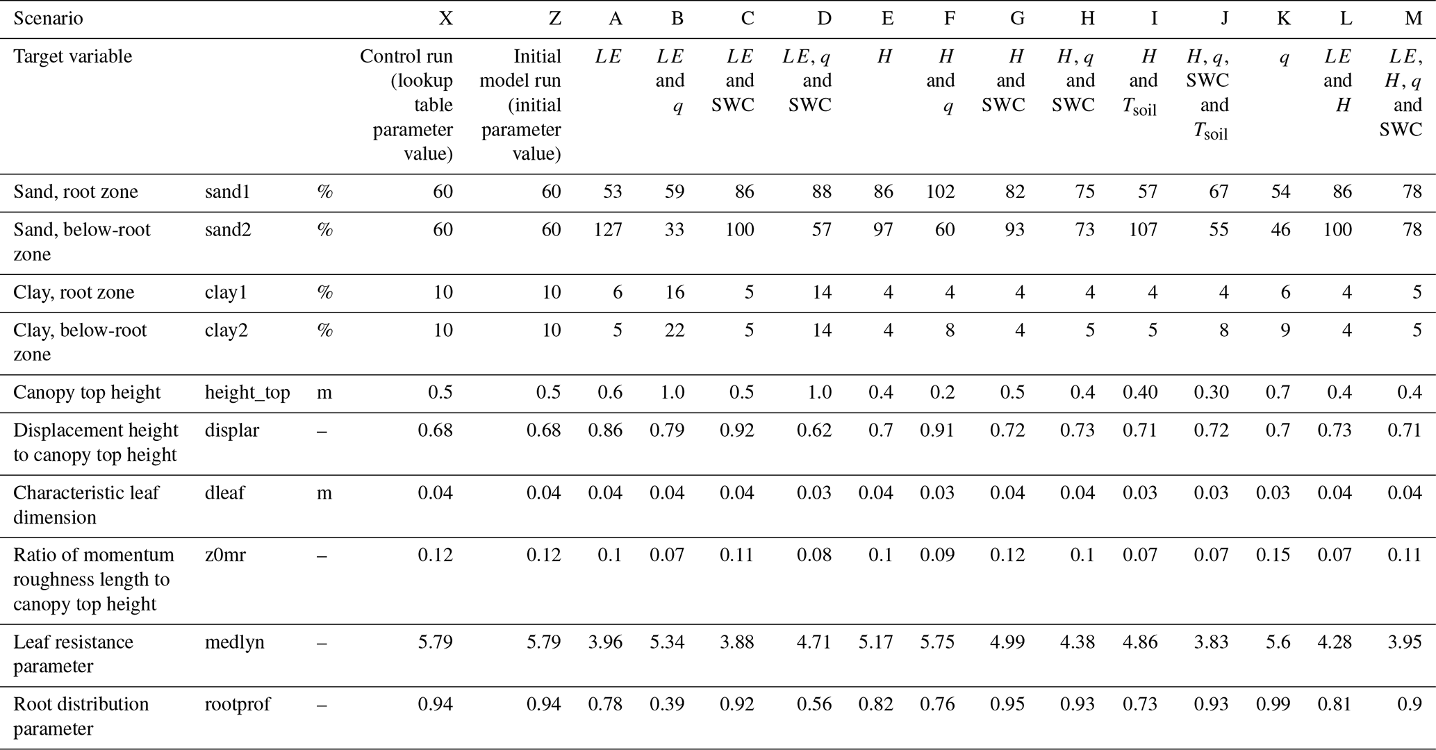
Table 1Lookup table with initial and optimized parameter values for all scenarios. The LAI and optical parameter values can be found in Tables S1 and S2 in the Supplement.
In CLM5, the soil and hydraulic parameters, including porosity, saturated hydraulic conductivity and the Clapp–Hornberger exponent B, in the functional relationships for retention and unsaturated hydraulic conductivity are derived from soil texture (percentage of sand/clay and organic matter fraction) in each soil layer (Lawrence et al., 2019a) using built-in pedotransfer functions. Measured soil texture was used as prior knowledge/initial values (Vasquez, 2013). These were slightly different from lookup table parameter values (Tables 1, S1, S2). The soil carbon density in the root zone was fixed at a value of 6 kg m−3, as this represents an organic matter content corresponding to the measured value of 4.5 % (Andreasen et al., 2020). Soil color determines a dry or saturated soil albedo (Fisher et al., 2019). Soil color was not included in the calibration because the parameter estimation tool was not able to handle parameter values as integers. The lookup parameter value of soil color for the field site is 13; we used this value in the simulations.
The a priori satellite-derived LAI and SAI values were aggregated from high-resolution input datasets (Cheng et al., 2021). According to our basic knowledge of the field site (Herbst et al., 2011), the a priori LAI values derived from satellite images seemed rather small. Therefore, we used initial values for the LAI from Herbst et al. (2011). We included all 12 of the monthly LAI parameters in the calibration. We used the SAI values from the lookup table and did not include them in the optimization. Initial values of the eight optical property parameters were defined according to the lookup table values.
We used a single plant functional type (PFT) “C3 Unmanaged Rainfed Crop” (Lawrence et al., 2019a) for a priori vegetation parameter values. The prescribed leaf orientation index for “C3 Unmanaged Rainfed Crop” of −0.3 was changed to −0.5, as this is the prescribed value for spring wheat (Lawrence et al., 2019a).
Parameter limits were given wide intervals to provide full freedom to the parameter optimization. Prior calibration parameter variability () was given as a standard deviation of 0.5 in the log space of the respective parameters.
In the calibration, we used seven different observation datasets (all at an hourly resolution) as optimization targets: Rn, Sout, LE, H, q, Tsoil and the SWC in the top soil layer. We considered 13 individual scenarios (A–M) in which calibration was carried out against different combinations of observation data types (Table 1). The scenarios were designed to study the value of hydrological data in an energy-based LSM and the reliability of respective LE and H observations. Rn and Sout were included as optimization targets to ensure a persistent match between observations and simulations of Rn and Sout.
The multi-objective function (ϕobservation) that is minimized by PEST is defined as the squared sum of weighted residuals:
where m is the number of observation groups in the given optimization; n is the number of respective Rn, Sout, LE, H, q, SWC and Tsoil observations; ω is the weight of the observations; and yobs and ysim are observed and simulated values, respectively. We ensured uniform weighting between the different observation groups to avoid single observation groups excessively dominating the parameter estimation.
Regularization was introduced in all calibrations by adding the regularization objective function (ϕregularization) to ϕobservation. As we used preferred value regularization, ϕregularization consists of the weighted least squares of the difference between the parameter value and the preferred (a priori) parameter values. Thus, the total objective function (ϕt) comprises the sum of the observation and the regularization objective functions:
where μ is the weight factor of the regularization objective function (Doherty, 2018a).
In mathematical regularization, we seek an “appropriate” fit, rather than the best possible fit, between simulations and observations (Doherty et al., 2010). An acceptable fit is specified by PHIMLIM, which defines a threshold value that the observation objective function must not fall below. By setting this threshold, a balanced optimization is obtained with respect to observations and prior parameter values. PHIMLIM was set 10 % higher than the lowest achieved objective function, and PHIMACCEPT was set 10 % higher than PHIMLIM, as recommend by Doherty (2018a).
The weights for the individual observations were assigned such that they were proportional to the standard deviation associated with the observation. The standard deviation was assumed to be 10 % of the absolute observation value. To ensure that all observation time steps had a balanced impact on the objective function, we developed a simple model of the observation weights of LE, H and q. Within this model optimization, larger observations are given a higher weight than smaller observations; hence, time steps where yobs≈0 are prevented from having an inappropriate high weight and, therefore, an inappropriate high impact on the objective function.
where aLE=1000, aH=1000, and aq=1. All SWC and Tsoil observations were given the same weight and, thus, were not dependent on the observation value.
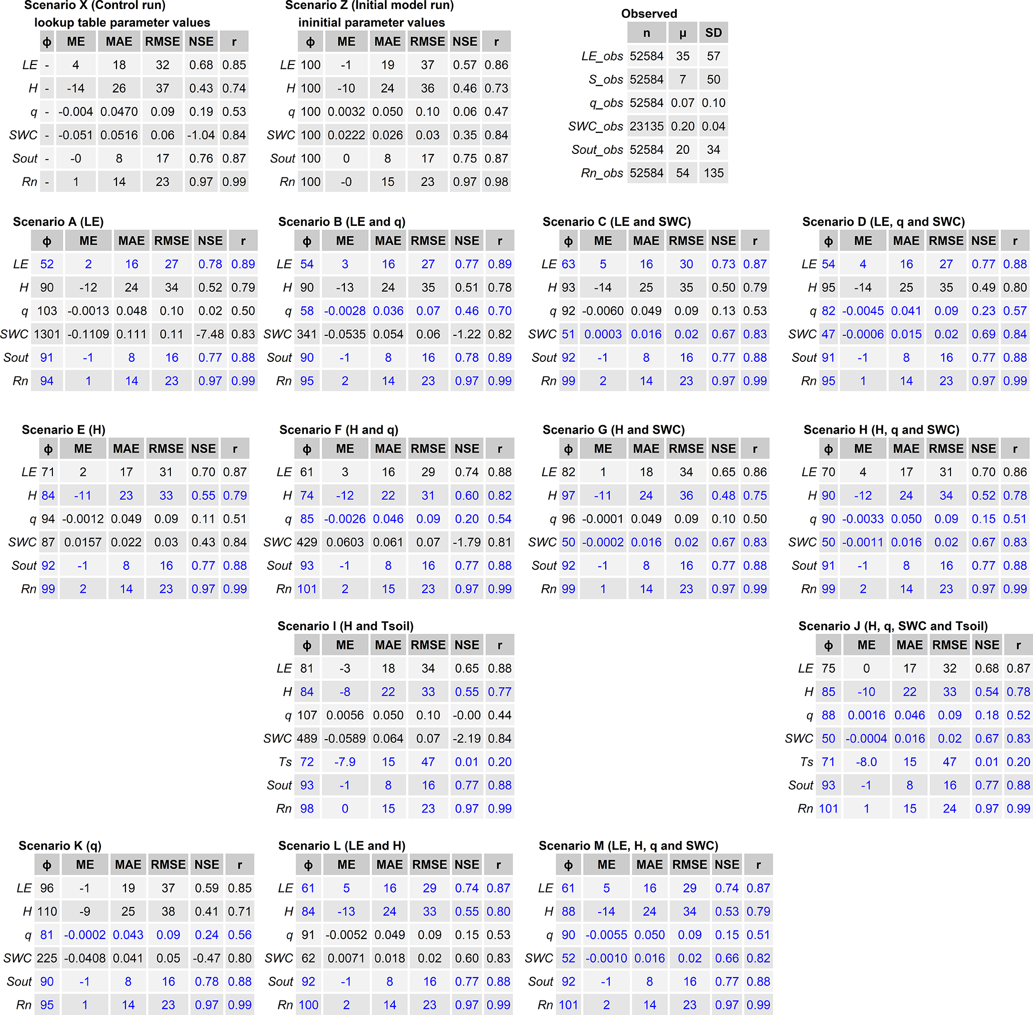
All calibration scenarios were assessed based on the mean error (ME), mean absolute error (MAE), root-mean-square error (RMSE), Nash–Sutcliffe efficiency (NSE) coefficient and Pearson correlation (r) coefficient for each of the six observation groups' LE, H, Rn, q, SWC and Tsoil.
Here, N is the number of observations in the given observation group. All summary statistics were calculated on an hourly time basis.
A small ME suggests that the overall model fit is not biased; however, positive and negative errors may cancel out, implying that ME may be a weak indicator of the goodness of model fit. Instead, the MAE may be a better indicator of model performance. The RMSE is a performance criteria that gives higher weight to large errors, as opposed to the MAE that weights all residuals equally. The innate character of the RMSE is very much related to the objective function. The NSE and r are both unitless, should ideally be as close to one as possible and are comparable across data types. The NSE is a measure of the model's ability to match the temporal variability, whereas the r is a measure of the strength of the linear relationship. For the ME, MAE and RMSE, the closer the metrics are to zero, the better the model performs. The optimized fluxes and states of the system are evaluated via those six metrics (including the objective function). It is important to keep in mind that the PEST optimization tool uses the objective function and that this does not necessarily improve all other metrics.
Aside from parameter estimation, the PEST software package contains a collection of utility programs for the calculation of the model parameter uncertainties developed under the assumption of linearity. Thus, the uncertainty estimates are approximations, but they can, nevertheless, provide useful information, even though the system may violate the assumptions (Doherty, 2015). The truncation point (or threshold) between the null and solution space is a generic mathematical concept that enables an investigation of model error (Doherty et al., 2010; Doherty, 2015).
To assess the parameter importance, we used the two statistics “identifiability” and “relative error variance reduction” (Doherty and Hunt, 2009) calculated by the IDENTPAR and GENLINPRED PEST utility programs. These statistics are based on the same concepts as those applied by mathematical regularization and rely on singular value decomposition of a weighted sensitivity matrix. In contrast to the one-at-a-time sensitivity analysis approach, identifiability and relative error variance reduction determine the significance of the parameters while taking the interactions among them into account (Doherty and Hunt, 2009).
The identifiability expresses the extent to which a parameter can be estimated uniquely based on the extent to which the parameter is located in the solution space and, hence, how much it is informed by available observation data. When the identifiability of a parameter is zero, the dataset possesses no information with respect to that parameter, and the uncertainty is not reduced through the calibration process. When the identifiability of a parameter is one, it does not mean that the parameter can be estimated without error, but it indicates that its potential for error is dominated by and originates from the noise of the observation data (Doherty and Hunt, 2009).
Table 2Summary statistics. The units of each variable are as follows: the NSE and r are unitless, the ME and MAE for H and LE are given in watts per square meter (W m−2), the ME and MAE for q are given in millimeters per hour (mm h−1), the ME and MAE for the SWC are given in cubic meters per cubic meter (m3 m−3), ϕ and the RMSE for H and LE are given in watts per square meter squared ((W m−2)2), ϕ and the RMSE for q are given in millimeters per hour squared ((mm h−1)2), and ϕ and the RMSE for the SWC are given in cubic meters per cubic meter squared ((m3 m−3)2). Blue color indicates that variables were included in the calibration for the given scenario.
The relative error variance reduction (ri) describes the extent to which the calibration process reduces the variance of a parameter from the pre-calibration level (Doherty and Hunt, 2009):
where is the post-calibration error variance associated with the estimation of parameter i and is its pre-calibration error variance assigned by expert knowledge.
To provide a basis for comparison, we ran a control simulation using CLM5's a priori (lookup table) parameter values (Scenario X). Additionally, a simulation was run (Scenario Z) in which some lookup table parameters values were replaced by observed parameter values. Table 1 presents the soil texture parameters and the plant functional type (PFT) parameters. The respective LAI and optical parameters can be found in Tables S1 and S2 in the Supplement. Lookup table and initial parameter values are listed along with the optimized parameters for all calibrated scenarios. Scenarios A, E and K are calibrations with LE, H and q, respectively, as targets. The remaining scenarios are multi-objective calibrations using different combinations of observational data types. The summary statistics are given in Table 2, which presents the following information: the top row shows the initial and control runs as well as statistics on the observed data; row no. 2 presents calibration results using LE as the target as well as results using LE combined with other measurement types as targets; row no. 3 is similar to row no. 2 but LE is substituted by H; row no. 4 is similar to row no. 3 but including Tsoil as the target variable; and the last row shows the results using different combinations of targets.

Figure 1Observed and simulated LE and H (daily mean for 2010–2015) for Scenario X (control run), Scenario D and Scenario E over a 1-year period (a–c) and (hourly mean for 2010–2015) over a 1-week period in June (d–f).
As was used indirectly to obtain incident longwave radiation for model forcing (Eq. 2), there is a good match between and and between and in the control run. To ensure that simulated and observed Rn and Sout agree in the optimization process, Rn and Sout were included in the objective function (Eq. 3) and given the same group weight as that for the other variables in the objective function. We included Rn and Sout in the objective function to ensure accordance between observed and simulated Rn and the shortwave radiation components. It is important to note that, in the control run and initial model run (scenarios X and Z), an excellent match between and was already obtained; therefore, we do not expect the metrics for Rn to improve in the calibrated scenarios (Table 1).
3.1 Analysis of the control run
Simulations based on lookup parameter values for the field site (Scenario X) highly overestimate daily H all year except in July and August (Fig. 1b). On the contrary, LE is underestimated during the cold season from September to April, especially in March and April (Fig. 1a). This model conceptualization fails to reproduce the correct partitioning between LE and H during the grain-filling and harvest period in July and August, when LE is highly overestimated (Fig. 1a) and H is underestimated (Fig. 1b).
Regarding the unsaturated zone variables, the control run (Scenario X) consistently simulates an overly high SWC level, although the dynamics match the observations fairly well (Fig. 2a). The model fails to capture the overall dynamics of q, including low- and high-flow events (Fig. 2b). For certain years, 2010 and 2011, snow periods are not simulated well (results not shown).
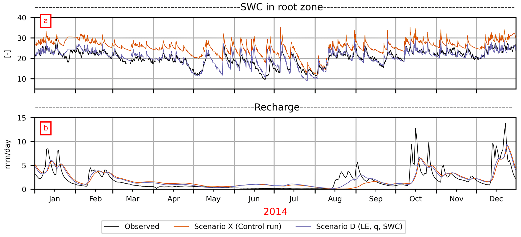
Figure 2Observed and simulated SWC and q for Scenario X (control run) and Scenario D in 2014.
As the turbulent fluxes have a distinct diurnal variation, we compare simulations and observations in Fig. 3 for 4 individual months. For the control run (Scenario X), the daytime LE values are slightly overestimated in June (Fig. 3b), whereas they are underestimated in all other months (Fig. 3a, c, d). For H, both the daytime and nighttime values are overestimated in all 4 months (Fig. 3e, f, g, h). Thus, CLM5 highly overestimates H based on lookup parameter values and is not capable of simulating negative nocturnal H (Figs. 1e and 3e, f, g, h). In winter, the CLM5 control run simulates small negative H during the night, but Hobs is much lower than Hsim (Fig. 3h).
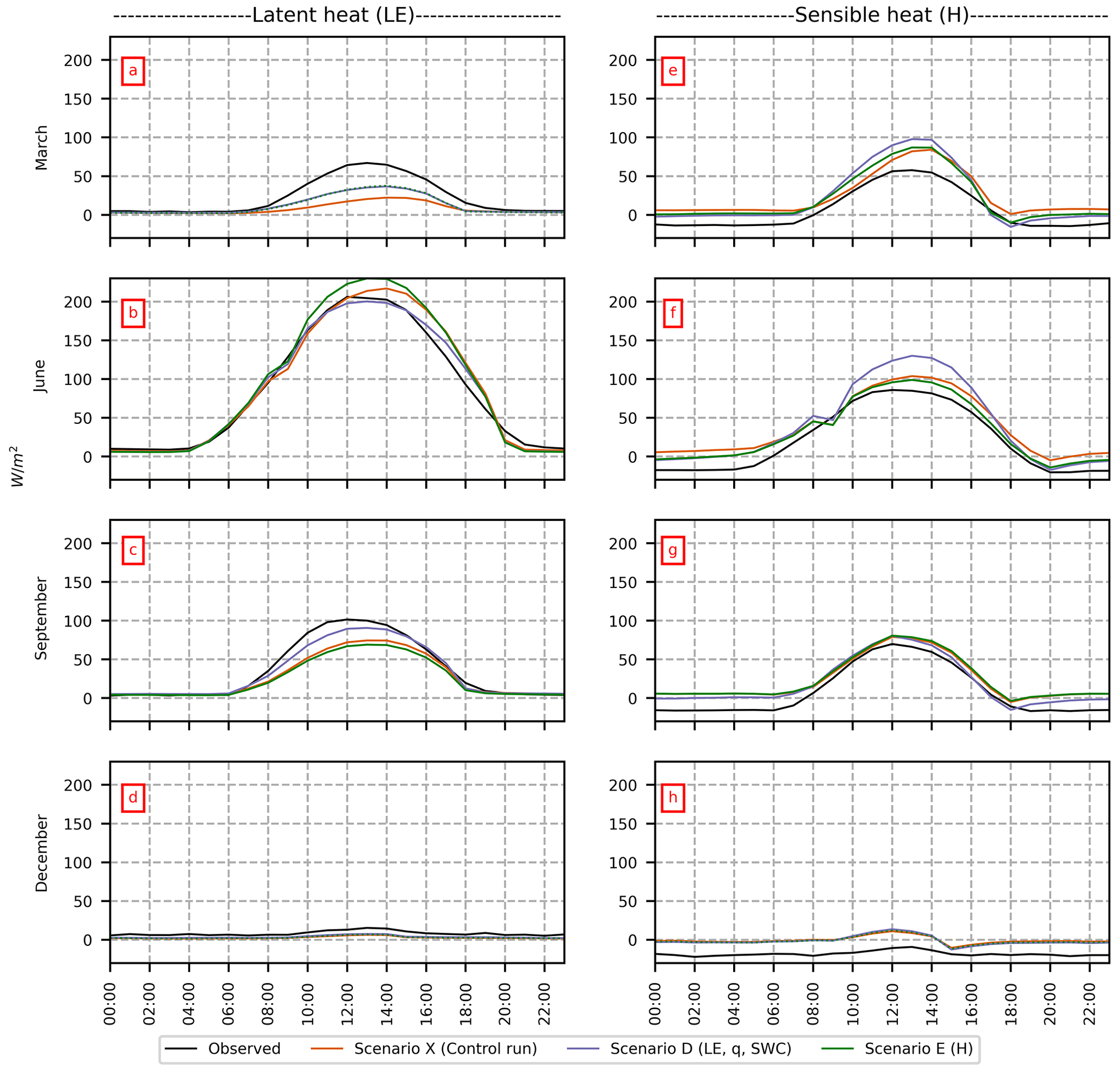
Figure 3Seasonal daily cycle of observed and simulated (hourly mean for 2010–2015) LE and H for Scenario X (control run), Scenario D and Scenario E.
3.2 Analysis of multi-objective calibration results
As expected, calibration enhances CLM5's ability to simulate the dynamics of the energy fluxes, recharge and soil moisture, although with a consistent overestimation of H (Fig. 1b, e).
LE and H are linked through the energy balance and the partitioning of incoming energy into LE and H. In most calibrated scenarios, optimization against either one of the turbulent fluxes improves the other as well. Thus, the inverse calibration improves the simulation of both LE and H. When comparing the initial model run (Scenario Z) with the calibrated scenarios in general, Hsim and Hobs match better in all of the calibrated scenarios (scenarios A–M) than in the control run (Table 2). This applies to most metric types but is most evident for ϕH, which is less than 100 in all scenarios (except Scenario K). This is the case regardless of whether H is used as calibration target (scenarios E–J, L and M) or not (scenarios A–D). In the same way as for H, Table 2 shows that the summary statistics for LE are likewise improved for all scenarios when compared with the initial model run.
Scenarios A and D are, as expected, best at capturing the reduction in LE in the harvest and grain-filling period in July and August. However, it is important to keep in mind that Fig. 1 shows the daily mean over a 6-year period, and the variation in the timing of harvest/grain fill will affect the visual comparison.
Figure 1d, e and f present results for the first week in June. When LE is used as target variable (Scenario A), H is overestimated; the inverse is observed if H is used as the target variable (Scenario E). The excess energy is placed on the other turbulent flux or on G (Fig. 1f).
Despite the improvement in both LEsim and Hsim, a clear discrepancy between Hsim and Hobs is found after calibration (Table 2); this is also seen for the single-objective optimization (Scenario E), as a bias of ME W m−2 is found. MEH is negative in all scenarios with a value of between −9 and −14 W m−2. This is a very high absolute value, especially compared with the mean value of the observations ( W m−2; Table 2). The bias of Hsim can also been seen in Fig. 1b, where the calibrated scenarios are not able to match mean daily Hobs and the simulated values are higher than observations for most of the year. The same discrepancies between simulations and observations can be seen in Fig. 3e, f, g and h, where hourly Hobs values are less than Hsim values for all scenarios and for all months, especially at night. We see from Fig. 1e that CLM5 overestimates the nighttime negative H values.
For Scenario D, LEsim matches LEobs nearly perfectly in June (Figs. 1a, 3b); however, during the remaining seasons (Fig. 3a, c, d), LEsim is underestimated. For example, the calibration of LE (Scenario A) only slightly improves the climatology of LE during March (Fig. 3a). There is only a slight difference in turbulent fluxes between scenarios A and D; thus, including hydrological observations in the objective function does not have much effect on the results.
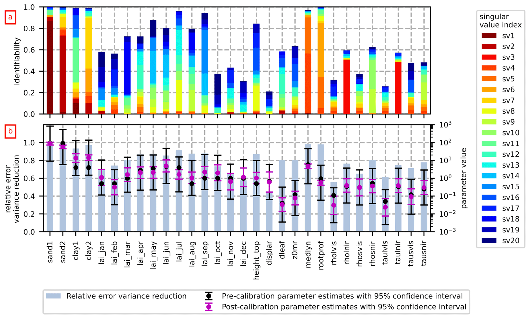
Figure 4The identifiability (a) and the relative error variance reduction and optimized parameter values (b) for Scenario D. The total height of the bars in panel (a) indicates the identifiability of each parameter, and the color-coding of each bar corresponds to the contribution of the singular values to the identifiability. The reader should note the logarithmic scale on the secondary y axis of panel (b).
As expected, the single-criteria optimization of LE (Scenario A) leads to the best summary statistics for LE (Table 2); however, for H, the best summary statistics are surprisingly obtained in Scenario F and not in Scenario E. In the same way, optimization against LE and q (Scenario B) gives better summary statistics for q than the single-objective optimization of q (ϕq=58 for Scenario B and ϕq=81 for Scenario K) and is capable of matching observed and simulated q to a better degree than other scenarios. However, in general, the dynamics of q are not well simulated in any of the scenarios, as reflected by the NSEq being less than 0.46 for all scenarios (Table 2).
The model is generally better at simulating the dynamics of LE compared with H and the hydrological observations, as evidenced by the NSE for the different scenarios (Table 2). This is also the case if LE is not included in the objective function. In all cases (except Scenario G), NSELE is higher than NSEq, NSESWC and NSEH (Table 2). To ensure that the heat and water budget are constrained to the same extent, we ran two scenarios that include Tsoil as a target variable in the calibration. A slight improvement in MEH (from −11 to −8 W m−2) is obtained from Scenario E to Scenario H, but MEH is still highly biased, and the remaining metrics for H are not improved when including Tsoil as the target variable.
The results demonstrate that it is important to include several data types in the optimization. Single-objective optimization against LE or H, respectively, leads to good results for the respective fluxes but deteriorates the simulation of the internal hydrological processes, especially the SWC. The absolute level of simulated SWCsim is too high in the control run (Scenario X) but becomes much better when using site-specific parameter values in the initial model run (Scenario Z) (not shown).
The information content of the different observation data types can be examined by comparing the model results of the different scenarios. When evaluating the model performance of scenarios A–D, it is evident that including q in the objective function (Scenario B) improves the fit of q (ϕq=103 for Scenario A and ϕq=58 for Scenario B) and the SWC (ϕswc=1301 for Scenario A and ϕswc=341 for Scenario B) while still maintaining strong agreement with LE observations (ϕ=52 for Scenario A and ϕLE=54 for Scenario B). On the other hand, including the SWC in the objective function (Scenario C) also improves q (ϕq=103 for Scenario A and ϕq=92 for Scenario C), although the match with LE observations becomes worse (ϕLE=52 for Scenario A to ϕLE=63 for Scenario C). When including both q and SWC in the calibration, a good fit of LE and the SWC as well as an acceptable agreement with q observations can be obtained (Scenario D). Scenario D leads to the best overall model results. Including the SWC in the parameter optimization leads to a good match between SWCobs and SWCsim (Fig. 2a).
Surprisingly, summary statistics (Table 2) do not change much when calibrating the dynamics of LE and H at the same time (scenarios L and M). H is simulated with low accuracy independently of whether LE is included in the objective function or not, and LE is simulated slightly worse in Scenario L than in Scenario A (ϕH=52 for Scenario A and ϕH=61 for Scenario L). Including all four data types in the optimization (Scenario M) still leads to a bias of H simulations.
The parameter response space of CLM5 is complex, and the impacts of the parameters estimated on water and energy fluxes vary with different parameter value combinations. In general, Scenario D gives the best results. Figure 4 shows the identifiability, the relative error variance reduction and the estimates of 30 parameters estimated for Scenario D. The total height of each bar in Fig. 4a is the identifiability of the pertinent parameter, and the color-coding of each bar corresponds to the contribution of different eigencomponents spanning the calibration solution space to the identifiability: warmer colors (red–yellow) correspond to singular values of smaller index (singular value of higher magnitude) and indicate that the parameter is less prone to measurement noise and more informed by observation data (Doherty, 2015).
The boundary between the solution and null subspaces for Scenario D was set to 20. The 30 parameters show a broad range of identifiability, and 14 of the 30 parameters are identifiable on the basis of the hourly observations of Rn, Sout, LE, q and SWC if a somewhat arbitrary qualitative identifiability level of 0.7 is chosen to mark the cutoff between identifiable and unidentifiable parameters. The 14 identifiable parameters are primarily the sand and clay fractions, the LAI in summer, height_top, medlyn and rootprof.
The parameters that have the highest identifiability and are mostly informed by data (warmer colors in Fig. 4) also have the highest relative error variance reduction. Hence, the information contained in the observation dataset constrains the identifiable parameters, whereas the unidentifiable parameters are, to a stronger degree, constrained by expert knowledge in the form of preferred values in the Tikhonov regularization. The parameter confidence intervals mostly decrease for the parameters that are more informed by data.
Figure 5 shows the optimized parameter values, i.e., the soil parameters (Fig. 5a), LAI (Fig. 5b) and optical parameters (Fig. 5c). The optimized values for the plant functional type (PFT) parameters can be found in Tables 1, S1 and S2. Additionally, Fig. 5 indicates how much the parameters have moved compared with the a priori lookup table values and the initial parameter values.
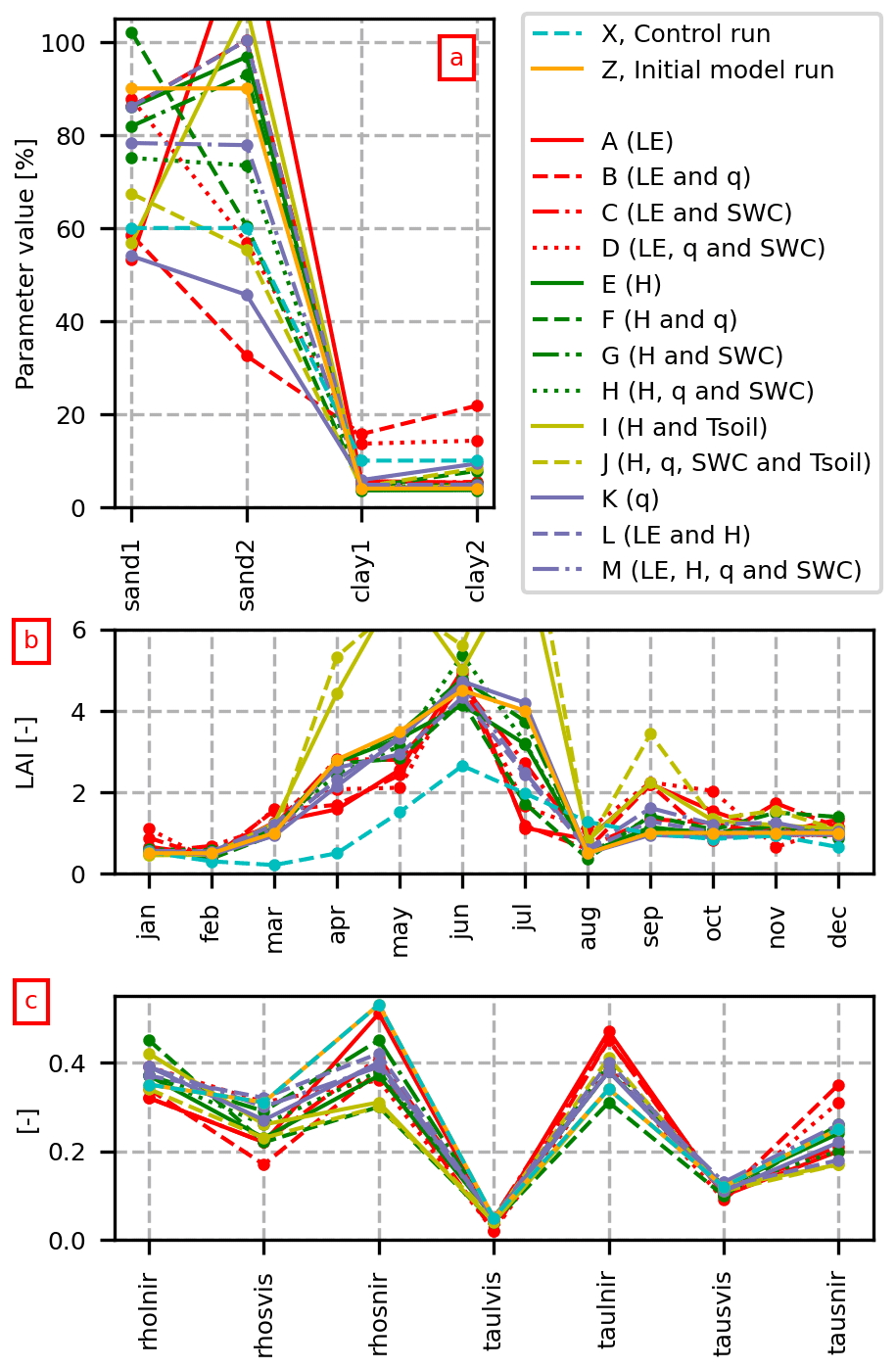
Figure 5Optimized parameter values for all scenarios for (a) soil parameters, (b) LAI and (c) optical parameters.
The a priori values for the PFT parameters are retrieved from global datasets, whereas the soil and vegetation phenology parameters are linked to the study site location (Herbst et al., 2011; Vasquez, 2013). The sand1 and clay1 variables determine the hydraulic properties of the root zone. The sand1 variable is highly informed by data (warmer colors in the identifiability plots in Fig. 4a), which is also seen from the narrow post-calibration confidence interval (Fig. 4b). According to the local information (Vasquez, 2013), the soil at the field site is sandy with a very low clay content. Most calibrated scenarios obtain reasonable soil texture values: the sand content mostly varies between the lookup table value of 60 % and up to 100 %, and the clay content is below 20 %. All scenarios that include q in the objective function (scenarios D, F, H, J, K and M) reduce the fraction of sand in the soil layer below the root zone (sand2). We know that this is incorrect and that the soil texture becomes coarser with depth (Haarder et al., 2015). All scenarios not including q in the objective function have an expected high sand content below the root zone (Fig. 5a). Scenario A, in contrast, has an unrealistic high value for the sand fraction of sand2. In general, the clay content is much less informed by data than sand (Fig. 4a)
All a priori values of the PFT parameters (except medlyn) are nearly identical for the different vegetation types in the lookup tables of CLM5 (Lawrence et al., 2019a). Thus, the specification of individual initial parameter values for each PFT is not possible.
The medlyn variable is a parameter of the stomatal conductance model. The parameter determines the degree of stomatal opening and has a critical impact on the stomatal responses in the soil–root–stem–leaf system. The optimal value for medlyn varies between 3.83 and 5.75 (Table 1).
The rootprof variable is the root distribution parameter that determines the root fraction in each soil layer, and it is critical for the SWC of the soil. This parameter is well informed by data, and the regularization strategy allows the parameter value to move away from the initial value.
The LAI shows similar patterns for all scenarios (Fig. 5b). As the LAI parameters are unidentifiable in cold months, the values do not deviate much from the preferred values. The optimized LAI values enhance energy partitioning of LE and H during the grain-filling and harvest phase in July and August (Fig. 1). The calibrated models match LE and H during the harvest period in July and August better than the control run.
The results presented show that multi-objective calibration considerably enhances the ability of CLM5 to represent both energy and hydrological processes. This result is expected to be applicable elsewhere, particularly in low-lying agricultural areas subject to high evapotranspiration. In line with Gupta et al. (1999), it was also demonstrated that optimization using a single-criterion objective function is less suitable, as the internal hydrological processes are not represented adequately. In contrast, multi-objective parameter estimation considerably enhances the ability of CLM5 to simulate observed energy and hydrology data. According to the summary statistics, Scenario D (calibrated against LE, q and SWC) gives the best overall representation of all data types (Table 2). Compared with the control run (Scenario X), Scenario D reduces the RMSE by 27 %, 2 %, 9 % and 31 % for LE, H, q and SWC, respectively.
In the following, we will discuss issues with respect to the energy and hydrology representation of the model, the calibration approach and the parameter uncertainty. However, to begin with, we will elaborate on the issue of land surface energy balance closure with respect to the calibration of an LSM as well as potential shortcomings of LSMs. Throughout the discussion, we will outline potential future work within the subject of the study.
4.1 Energy balance closure
The eddy covariance (EC) method is generally regarded as the best practical method for measuring turbulent energy fluxes at the land surface; however, numerous studies have documented the lack of energy balance closure (Foken et al., 2006; Franssen et al., 2010; Stoy et al., 2013). As measurements of Rn are generally trusted, an underestimation of the turbulent fluxes appears likely because the sum of the energy fluxes is less than Rn (Foken et al., 2011). The observation data from the field site (Ringgaard et al., 2011) show that incoming available energy (Rn minus G) on average exceeds the turbulent energy fluxes (LE and H) by 21 %; thus, the data are subject to a land surface energy imbalance (Denager et al., 2020). As LSMs conserve energy, the conclusions from LSM calibration studies using turbulent fluxes as target variables rest on the premise of closure of the observed energy fluxes. As it is not possible to match LEobs and Hobs simultaneously, scenarios L and M are fundamentally incorrect.
CLM5 simulates LE and H explicitly through the Monin–Obukhov similarity theory. Nonetheless, the regularization approach used in this study fails to identify parameter values to match uncorrected Hobs with Hsim (Scenario E). It is especially challenging to match negative H during winter and nocturnal periods, when the overlying air is warmer than the surface and sensible heat is, therefore, transported downwards (Figs. 1e and 3e, f, g, h). There may be structural limitations to CLM5 that prevent a good match to H. However, as the observed incoming and outgoing energy is imbalanced (Denager et al., 2020) and the model maintains Rn (Eq. 1), there is excess energy in the model, which CLM5 transmits to H and G. G is often considered to be a residual term for closing the energy balance in CLM5 (e.g., Kracher et al., 2009). Denager et al. (2020) concluded, by comparison to water balance measurements, that the imbalance of the EC method at the specific field site is, to a lesser degree, caused by errors in the LE estimates but can mainly be attributed to errors in the other energy flux components or unaccounted for effects.
Contrary to this study, many studies have tested LSMs using corrected flux observations of H and LE that fulfill energy closure (Carrillo-Rojas et al., 2020; Davison et al., 2016; Pauwels and De Lannoy, 2011; Larsen et al., 2016; Dombrowski et al., 2022). A few studies have tested LSMs using both corrected and uncorrected turbulent fluxes (Chen et al., 2018), but some studies do not indicate whether turbulent energy fluxes have been corrected or not (De Lannoy et al., 2011; Göhler et al., 2013; Hou et al., 2012). Chen et al. (2018) applied both corrected and uncorrected LE and H from FLUXNET to test a point-scale CLM4.5 over open sites; they found that simulations matched uncorrected LE better than corrected LE, and, as energy-balance correction methods increase the LE values, CLM4.5 underestimated FLUXNET-corrected LE.
4.2 Model physics in LSMs
In this study, we have shown that running the model with soil parameters that have been measured (and are therefore likely correct), i.e., Scenario Z, did not lead to improved model performance, which can potentially be interpreted as pointing to deficiencies in the model physics. More and more advanced descriptions of the processes have been built into LSM codes. This induces heavily increased model complexity and expands the associated number of parameters in the model equations (Mendoza et al., 2014). The parameter optimization in complex models is complicated, and there is a possibility that LSMs may not be parameterized appropriately. Several authors have contested the complexity of LSMs (Franks et al., 1999; Clark et al., 2015; McCabe et al., 2005; Williams et al., 2009) and suggested a reassessment of the structure and process representations. An overall simplification of the LSMs would enable a more profound parameter optimization and utilization of measured data. This would lead to more parsimonious LSMs, and utilizing the well-establish model evaluation within hydrology, considering uncertainties in data, model parameters and conceptual understanding (Refsgaard et al., 2021), would enhance the model evaluation of LSMs. Therefore, the hydrology and LSM modeling communities could benefit even more from each other (Clark et al., 2015).
4.3 Value of observation data
Physically, LE depends on both energy flux and water availability. Aside from LE, moisture information is clearly central to the optimization of the internal hydrological processes of CLM5. Other studies have also shown the appropriateness of the SWC in optimizing the hydrological state in LSMs (Zhang et al., 2017; De Lannoy et al., 2011). Similar to LE, groundwater recharge, q, also describes the water exchange; however, as long as LE data are available, q data only provide minor additional information to the calibration.
Data uncertainty has been discussed in Denager et al. (2020), and we are generally confident with the accuracy of our forcing and hydrological data. To improve the simulation of soil water flow in LSMs, we followed the suggestion of Rosero et al. (2010) and used percolation observations in the parameter optimization process. To capture the diurnal dynamics of energy and water fluxes, the optimization is based on hourly time steps. However, given the design of the lysimeters at the field site, where recharge water is collected at a sloping face at the bottom of the lysimeters, there may be a temporal mismatch between model simulations and observations. Although each of the four lysimeters has a surface area of 3.2 m × 3.88 m, their total area is much smaller than the footprint of the EC system.
4.4 Calibration approach
As 6 years of observations are available for all major water and energy balance components at the field site, there is the potential to studying the long-term effects on the seasonal energy and water fluxes and variables. However, the target of the applied calibration approach is the dynamics of the 24 h cycle of hourly observations, rather than the seasonal energy and water balance components.
Sun et al. (2013) found that parameter optimization using PEST only led to small improvements in performance of CLM4.0. In the present study, we were able to obtain considerable improvements by parameter optimization using singular value decomposition and Tikhonov regularization implemented in the PEST software package. This approach is more computationally effective than general Bayesian approaches that require a large number of model simulations to estimate parameter and predictive uncertainty, such as the stochastic Markov chain Monte Carlo inversion of CLM4 presented by Sun et al. (2013). Another approach was presented by Zhang et al. (2017), who evaluated different data assimilation methods for soil texture parameter estimation in the CLM.
4.5 Evaluation of optimal parameters values
Some CLM5 parameters, e.g., LAI and height_top, are physically meaningful and can be inferred directly from observations, whereas other parameters, e.g., displar, dleaf, medlyn, rootprof and z0mr can be viewed as conceptual representations for which useful values cannot be directly measured.
Aside from the stomatal resistance, the LAI also directly controls actual evapotranspiration, and, as the sum of LE and H is constrained by the energy preservation in CLM5, the LAI consequently determines both LE and H.
Theoretically, the LAI should not change between calibration scenarios, and most scenarios show very similar LAI and SAI values. Scenarios A–D show well-constrained LAIjun values of between 4.14 and 5.37. We did not consider SAI parameters as adjustable parameters, but preliminary model calibrations including SAI showed that the decreases in LAIjul and LAIaug were compensated for by an increase in SAIjul and SAIaug in nearly all scenarios. However, we do not expect the SAI to have a considerable influence on turbulent fluxes and hydrological variables. The increase in the LAI in some scenarios in September probably reflects emerging cover crop.
When CLM5 is run in satellite phenology mode, it is not capable of simulating the year-to-year variation in germination, leaf emergence, harvest, etc., as all years are assumed to follow the same pattern. The energy partitioning in July and August is simulated better in some years than in others, but, despite the alignment of distinct yearly phenology in CLM5, the abrupt decrease in LE (averaged over 6 years) at grain filling/harvest is quite well simulated (Fig. 1a). Calibration of CLM5 with the inclusion of the biogeochemistry (BGC) model is beyond the scope of this paper; however, as CLM5-BGC applies carbon and nitrogen cycle functionality, it replaces phenology with prognostic variables. These variables change dynamically with meteorological forcing, soil moisture and nutrient availability (Cheng et al., 2021). Inclusion of the BGC module in CLM5 would further enable simulations of cover crops schemes (Boas et al., 2021). According to Boas et al. (2021), the cover crop scheme helped to match the observed energy balance.
It is a large disadvantage when calibrating LSMs that many important parameters are often hard coded (Davison et al., 2016). Adjusting those hard-coded parameters requires manual alteration of the appropriate code lines and subsequent recompiling before every parameter trial in the calibration routine. This limits the calibration process and the ability of the model to describe important processes (Mendoza et al., 2014).
The model uses pedotransfer functions to estimate the soil hydraulic properties, which is a useful approach for large-scale applications. However, for local-scale applications, as in this study, it would have been more appropriate to be able to specify the hydraulic properties directly. We observed that CLM5 overestimates the recharge during spring and summer, indicating that the representation of the hydraulic properties is inadequate when estimated from pedotransfer functions of optimized soil texture. A large number of former studies regarding parameter estimation and parameter sensitivity in CLM5 have related their analysis to the hydrologic parameters (e.g., hydraulic conductivity) rather than evaluating the model parameters in the pedotransfer functions (e.g., percentage of sand and clay) (Hou et al., 2012; Göhler et al., 2013; Huang et al., 2013; Sun et al., 2013).
De Lannoy et al. (2011) analyzed the effect of different soil texture specifications on simulations of SWC, LE and H using CLM3.5 and concluded that the impact of soil texture on energy fluxes is minor but the impact on water storage characteristics is significant. The present study found that the soil texture parameters (especially in the root zone) are also identifiable in the single-objective calibration of Scenario A.
It should be noted that, although soil texture is defined as a proportion of sand and clay (and therefore has the unit of percentage), individual values of sand or clay > 100 % are conceivable in CLM5, as the parameter intervals were set >100 %. In some scenarios, we obtain a sum of sand and clay slightly above 100 %, but this is not considered a critical issue, as the textural percentages are only used as parameters in the pedotransfer function for the hydraulic properties.
Similar to other sensitivity studies of CLM, we find that the stomatal conductance parameter (medlyn) and the soil parameters are highly significant (Göhler et al., 2013). In contrast, Hou et al. (2012) and Huang et al. (2013) found that subsurface generation parameters (distribution of surface runoff with depth, max subsurface drainage and specific yield) are the most important parameters for LE, H and runoff in CLM4, whereas soil texture parameters (Clapp and Hornberger parameter b and porosity) are of secondary significance. However, the parameters that are most sensitive can vary from site to site and from season to season, and the significance of parameters also depends on which target variable is considered. As our cropland field site has a shallow root zone, the unsaturated zone parameters (e.g., soil texture in the top layer) became more important.
The a priori value of 0.943 for rootprof is similar for all grass and crop PFTs (Lawrence et al., 2019a). Therefore, the off-the-shelf CLM5 does not distinguish root density for different types of grasses and crops. There is the clear possibility to constrain individual rootprof parameter values for different land-cover types. We found the rootprof parameter to be highly identifiable and, thus, highly informed by LE, q and SWC observation data. Our optimized values of the rootprof parameter for the scenarios including the SWC in the objective function (scenarios B and C) are substantially different from the a priori values (rootprof = 0.39 for Scenario B and rootprof = 0.56 for Scenario C). However, the optimized values of rootprof seem reasonable, as they imply an increase in the root density near the surface and a reduction at deeper soil layers, which fit well with the spring and winter barley cultivated at the agricultural field.
In this study, we explore how parameter estimation techniques can be used to improve the hydrological processes in a state-of-the-art LSM. The results indicate that mathematical regularization is a compelling method to improve the current practice of using lookup tables to define parameter values in LSMs.
Using the case study of an agricultural field in western Denmark with 6 years of extensive observations, we demonstrate that calibrating a point-scale CLM5 using (i) multi-objective calibration, (ii) truncated singular value decomposition and (iii) Tikhonov regularization employing combinations of hourly time series of latent heat, sensible heat, soil moisture and groundwater recharge from 2010 to 2015 can considerably improve the characterization of the energy and water fluxes.
The control run overestimated the soil moisture by more than 10 %; however, we found that parameter optimization of CLM5 using soil moisture data enhanced the ability of the model to describe the temporal patterns of moisture storage within the root zone. Calibration also considerably improved the energy partitioning of LE and H during the summer period and revealed good reproduction of observed and simulated LE and H during the grain-filling and harvest period in July and August.
Nevertheless, we found that H was biased the rest of the year, as the simulated H was clearly overestimated. It was not possible to fine-tune parameters to match the observed H, which suggests that the observed H needs to be corrected to match simulations.
Additionally, we evaluated the post-calibration uncertainties of the model parameters using the identifiability and relative error variance reduction statistics. Identifiability indicates the extent to which the parameter is informed by observation data. Using LE, q and SWC as target variables, we found that the identifiable parameters were soil texture, monthly LAI in summer, the stomatal conductance model parameter (medlyn) and the root distribution parameter (rootprof).
Our results highlight the necessity for parameter calibration using available observations of energy and hydrological fluxes to obtain an optimal parameter set for CLM5. We anticipate that the results from this study will contribute to improvements in the model characterization of water and energy fluxes, especially when EC flux data are available.
The forcing and calibration data from the site can be obtained from the corresponding author upon reasonable request.
The supplement related to this article is available online at: https://doi.org/10.5194/hess-27-2827-2023-supplement.
TD, TOS, MCL and KHJ designed the study. TD carried out all numerical modeling and analyses and also designed the figures. TD was primarily responsible for writing the manuscript. All authors discussed the results and provided critical feedback on the manuscript drafts.
The contact author has declared that none of the authors has any competing interests.
Publisher's note: Copernicus Publications remains neutral with regard to jurisdictional claims in published maps and institutional affiliations.
We are very thankful for the opportunities that this donation provided. Additionally, we would like to thank Theresa Boas and Lukas Strebel (Forschungszentrum Jülich) and Rena Meyer (the University of Oldenburg) for their help and guidance.
This research has been supported by the Villum Foundation.
This paper was edited by Luis Samaniego and reviewed by three anonymous referees.
Andreasen, M., Jensen, K. H., Bogena, H., Desilets, D., Zreda, M., and Looms, M. C.: Cosmic Ray Neutron Soil Moisture Estimation Using Physically Based Site-Specific Conversion Functions, Water Resour. Res., 56, 1–20, https://doi.org/10.1029/2019WR026588, 2020.
Boas, T., Bogena, H., Grünwald, T., Heinesch, B., Ryu, D., Schmidt, M., Vereecken, H., Western, A., and Franssen, H. J. H.: Improving the representation of cropland sites in the Community Land Model (CLM) version 5.0, Geosci. Model Dev., 14, 573–601, https://doi.org/10.5194/gmd-14-573-2021, 2021.
Bogena, H. R., Montzka, C., Huisman, J. A., Graf, A., Schmidt, M., Stockinger, M., von Hebel, C., Hendricks-Franssen, H. J., van der Kruk, J., Tappe, W., Lücke, A., Baatz, R., Bol, R., Groh, J., Pütz, T., Jakobi, J., Kunkel, R., Sorg, J., and Vereecken, H.: The TERENO-Rur Hydrological Observatory: A Multiscale Multi-Compartment Research Platform for the Advancement of Hydrological Science, Vadose Zone J., 17, 1–22, https://doi.org/10.2136/vzj2018.03.0055, 2018.
Bogena, H. R., Schrön, M., Jakobi, J., Ney, P., Zacharias, S., Andreasen, M., Baatz, R., Boorman, D., Duygu, M. B., Eguibar-Galán, M. A., Fersch, B., Franke, T., Geris, J., González Sanchis, M., Kerr, Y., Korf, T., Mengistu, Z., Mialon, A., Nasta, P., Nitychoruk, J., Pisinaras, V., Rasche, D., Rosolem, R., Said, H., Schattan, P., Zreda, M., Achleitner, S., Albentosa-Hernández, E., Akyürek, Z., Blume, T., Del Campo, A., Canone, D., Dimitrova-Petrova, K., Evans, J. G., Ferraris, S., Frances, F., Gisolo, D., Güntner, A., Herrmann, F., Iwema, J., Jensen, K. H., Kunstmann, H., Lidón, A., Looms, M. C., Oswald, S., Panagopoulos, A., Patil, A., Power, D., Rebmann, C., Romano, N., Scheiffele, L., Seneviratne, S., Weltin, G., and Vereecken, H.: COSMOS-Europe: a European network of cosmic-ray neutron soil moisture sensors, Earth Syst. Sci. Data, 14, 1125–1151, https://doi.org/10.5194/essd-14-1125-2022, 2022.
Carrillo-Rojas, G., Schulz, H. M., Orellana-Alvear, J., Ochoa-Sánchez, A., Trachte, K., Célleri, R., and Bendix, J.: Atmosphere-surface fluxes modeling for the high Andes: The case of páramo catchments of Ecuador, Sci. Total Environ., 704, 135372, https://doi.org/10.1016/j.scitotenv.2019.135372, 2020.
Chen, L., Dirmeyer, P. A., Guo, Z., and Schultz, N. M.: Pairing FLUXNET sites to validate model representations of land-use/land-cover change, Hydrol. Earth Syst. Sci., 22, 111–125, https://doi.org/10.5194/hess-22-111-2018, 2018.
Cheng, Y., Huang, M., Zhu, B., Bisht, G., Zhou, T., Liu, Y., Song, F., and He, X.: Validation of the Community Land Model Version 5 Over the Contiguous United States (CONUS) Using In Situ and Remote Sensing Data Sets, J. Geophys. Res.-Atmos., 126, 1–27, https://doi.org/10.1029/2020JD033539, 2021.
Clark, M. P., Fan, Y., Lawrence, D. M., Adam, J. C., Bolster, D., Gochis, D. J., Hooper, R. P., Kumar, M., Leung, L. R., Mackay, D. S., Maxwell, R. M., Shen, C., Swenson, S. C., and Zeng, X.: Improving the representation of hydrologic processes in Earth System Models, Water Resour. Res., 1–27, https://doi.org/10.1002/2015WR017096, 2015.
Dai, Y., Zeng, X., Dickinson, R. E., Baker, I., Bonan, G. B., Bosilovich, M. G., Denning, A. S., Dirmeyer, P. A., Houser, P. R., Niu, G., Oleson, K. W., Schlosser, C. A., and Yang, Z. L.: The common land model, B. Am. Meteorol. Soc., 84, 1013–1023, https://doi.org/10.1175/BAMS-84-8-1013, 2003.
Davison, B., Pietroniro, A., Fortin, V., Leconte, R., Mamo, M., and Yau, M. K.: What is missing from the prescription of hydrology for land surface schemes?, J. Hydrometeorol., 17, 2013–2039, https://doi.org/10.1175/JHM-D-15-0172.1, 2016.
De Lannoy, G. J. M., Ufford, J., Sahoo, A. K., Dirmeyer, P., and Houser, P. R.: Observed and simulated water and energy budget components at SCAN sites in the lower Mississippi Basin, Hydrol. Process., 25, 634–649, https://doi.org/10.1002/hyp.7855, 2011.
Demirel, M. C., Mai, J., Mendiguren, G., Koch, J., Samaniego, L., and Stisen, S.: Combining satellite data and appropriate objective functions for improved spatial pattern performance of a distributed hydrologic model, Hydrol. Earth Syst. Sci., 22, 1299–1315, https://doi.org/10.5194/hess-22-1299-2018, 2018.
Denager, T., Looms, M. C., Sonnenborg, T. O., and Jensen, K. H.: Comparison of evapotranspiration estimates using the water balance and the eddy covariance methods, Vadose Zone J., 19, 1–21, https://doi.org/10.1002/vzj2.20032, 2020.
Doherty, J.: Calibration and Uncertainty Analysis for Complex Environmental Models – The PEST book, Watermark Numerical Computing, ISBN 978-0-9943786-0-6, 2015.
Doherty, J.: PEST – Model-Independent Parameter Estimation – User manual Part I, Watermark Numerical Computing, https://pesthomepage.org/documentation (last access: 19 July 2023), 2018a.
Doherty, J.: PEST – Model-Independent Parameter Estimation – User manual Part II, Watermark Numerical Computing, https://pesthomepage.org/documentation (last access: 19 July 2023), 2018b.
Doherty, J. and Hunt, R. J.: Two statistics for evaluating parameter identifiability and error reduction, J. Hydrol., 366, 119–127, https://doi.org/10.1016/j.jhydrol.2008.12.018, 2009.
Doherty, J., Hunt, R. J., and Tonkin, M.: Approaches to Highly Parameterized Inversion: A Guide to Using PEST for Model-Parameter and Predictive-Uncertainty Analysis, S. Geological Survey Scientific Investigations Report, 2010–5211, 71 p., 2010.
Dombrowski, O., Brogi, C., Hendricks Franssen, H.-J., Zanotelli, D., and Bogena, H.: CLM5-FruitTree: a new sub-model for deciduous fruit trees in the Community Land Model (CLM5), Geosci. Model Dev., 15, 5167–5193, https://doi.org/10.5194/gmd-15-5167-2022, 2022.
Fisher, R. A., Wieder, W. R., Sanderson, B. M., Koven, C. D., Oleson, K. W., Xu, C., Fisher, J. B., Shi, M., Walker, A. P., and Lawrence, D. M.: Parametric Controls on Vegetation Responses to Biogeochemical Forcing in the CLM5, J. Adv. Model. Earth Syst., 11, 2879–2895, https://doi.org/10.1029/2019MS001609, 2019.
Foken, T., Wimmer, F., Mauder, M., Thomas, C., and Liebethal, C.: Some aspects of the energy balance closure problem, Atmos. Chem. Phys., 6, 4395–4402, https://doi.org/10.5194/acp-6-4395-2006, 2006.
Foken, T., Aubinet, M., Finnigan, J. J., Leclerc, M. Y., Mauder, M., and Paw U, K. T.: Results of a panel discussion about the energy balance closure correction for trace gases, B. Am. Meteorol. Soc., 92, 13–18, https://doi.org/10.1175/2011BAMS3130.1, 2011.
Franks, S. W., Beven, K. J., Quinn, P. F., and Wright, I. R.: On the sensitivity of soil-vegetation-atmosphere transfer (SVAT) schemes: Equifinality and the problem of robust calibration, Agr. Forest Meteorol., 86, 63–75, https://doi.org/10.1016/S0168-1923(96)02421-5, 1999.
Franssen, H. J. H., Stöckli, R., Lehner, I., Rotenberg, E., and Seneviratne, S. I.: Energy balance closure of eddy-covariance data: A multisite analysis for European FLUXNET stations, Agr. Forest Meteorol., 150, 1553–1567, https://doi.org/10.1016/j.agrformet.2010.08.005, 2010.
Göhler, M., Mai, J., and Cuntz, M.: Use of eigendecomposition in a parameter sensitivity analysis of the Community Land Model, J. Geophys. Res.-Biogeo., 118, 904–921, https://doi.org/10.1002/jgrg.20072, 2013.
Guo, L. and Lin, H.: Critical Zone Research and Observatories: Current Status and Future Perspectives, Vadose Zone J., 15, 1–14, https://doi.org/10.2136/vzj2016.06.0050, 2016.
Gupta, H. V., Bastidas, L. A., Sorooshian, S., Shuttleworth, W. J., Yang, Z. L., Bastidas, L. A., Sorooshian, S., Shuttleworth, W. J., and Yang, Z. L.: Parameter estimation of a land surface scheme using multicriteria methods, J. Geophys. Res.-Atmos., 104, 19491–19503, https://doi.org/10.1029/1999JD900154, 1999.
Haarder, E. B., Jensen, K. H., Binley, A., Nielsen, L., Uglebjerg, T. B., and Looms, M. C.: Estimation of Recharge from Long-Term Monitoring of Saline Tracer Transport Using Electrical Resistivity Tomography, Vadose Zone J., 14, 1–13, https://doi.org/10.2136/vzj2014.08.0110, 2015.
Herbst, M., Friborg, T., Ringgaard, R., and Soegaard, H.: Catchment-wide atmospheric greenhouse gas exchange as influenced by land use diversity, Vadose Zone J., 10, 67–77, https://doi.org/10.2136/vzj2010.0058, 2011.
Hou, Z., Huang, M., Leung, L. R., Lin, G., and Ricciuto, D. M.: Sensitivity of surface flux simulations to hydrologic parameters based on an uncertainty quantification framework applied to the Community Land Model, J. Geophys. Res.-Atmos., 117, 1–18, https://doi.org/10.1029/2012JD017521, 2012.
Huang, M., Hou, Z., Leung, L. R., Ke, Y., Liu, Y., Fang, Z., and Sun, Y.: Uncertainty analysis of runoff simulations and parameter identifiability in the community land model: Evidence from MOPEX basins, J. Hydrometeorol., 14, 1754–1772, https://doi.org/10.1175/JHM-D-12-0138.1, 2013.
Jefferson, J. L., Gilbert, J. M., Constantine, P. G., and Maxwell, R. M.: Reprint of: Active subspaces for sensitivity analysis and dimension reduction of an integrated hydrologic model, Comput. Geosci., 90, 78–89, https://doi.org/10.1016/j.cageo.2015.11.002, 2016.
Jensen, K. H. and Refsgaard, J. C.: HOBE: The Danish Hydrological Observatory, Vadose Zone J., 17, 1–24, https://doi.org/10.2136/vzj2018.03.0059, 2018.
Kracher, D., Mengelkamp, H. T., and Foken, T.: The residual of the energy balance closure and its influence on the results of three SVAT models, Meteorol. Z., 18, 647–661, https://doi.org/10.1127/0941-2948/2009/0412, 2009.
Krinner, G., Viovy, N., de Noblet-Ducoudré, N., Ogée, J., Polcher, J., Friedlingstein, P., Ciais, P., Sitch, S., and Prentice, I. C.: A dynamic global vegetation model for studies of the coupled atmosphere-biosphere system, Global Biogeochem. Cy., 19, 1–33, https://doi.org/10.1029/2003GB002199, 2005.
Lane, R. A., Freer, J. E., Coxon, G., and Wagener, T.: Incorporating Uncertainty Into Multiscale Parameter Regionalization to Evaluate the Performance of Nationally Consistent Parameter Fields for a Hydrological Model, Water Resour. Res., 57, 1–19, https://doi.org/10.1029/2020WR028393, 2021.
Larsen, M. A. D. D., Refsgaard, J. C., Jensen, K. H., Butts, M. B., Stisen, S., and Mollerup, M.: Calibration of a distributed hydrology and land surface model using energy flux measurements, Agric. Forest Meteorol., 217, 74–88, https://doi.org/10.1016/j.agrformet.2015.11.012, 2016.
Lawrence, D., Fisher, R., Koven, C., Oleson, K., Swenson, S., and Vertenstein, M.: CLM5 Documentation, National Center for Atmospheric Research (NCAR), Boulder, Colorado, https://www.cesm.ucar.edu/models/cesm2/land/CLM50_Tech_Note.pdf (last access: 19 July 2023), 337 pp., 2019a.
Lawrence, D., Fisher, R. A., Koven, C. D., Oleson, K. W., Swenson, S. C., Bonan, G., Collier, N., Ghimire, B., van Kampenhout, L., Kennedy, D., Kluzek, E., Lawrence, P. J., Li, F., Li, H., Lombardozzi, D., Riley, W. J., Sacks, W. J., Shi, M., Vertenstein, M., Wieder, W. R., Xu, C., Ali, A. A., Badger, A. M., Bisht, G., van den Broeke, M., Brunke, M. A., Burns, S. P., Buzan, J., Clark, M., Craig, A., Dahlin, K., Drewniak, B., Fisher, J. B., Flanner, M., Fox, A. M., Gentine, P., Hoffman, F., Keppel-Aleks, G., Knox, R., Kumar, S., Lenaerts, J., Leung, L. R., Lipscomb, W. H., Lu, Y., Pandey, A., Pelletier, J. D., Perket, J., Randerson, J. T., Ricciuto, D. M., Sanderson, B. M., Slater, A., Subin, Z. M., Tang, J., Thomas, R. Q., Val Martin, M., Zeng, X., Kampenhout, L., Kennedy, D., Kluzek, E., Lawrence, P. J., Li, F., Li, H., Lombardozzi, D., Riley, W. J., Sacks, W. J., Shi, M., Vertenstein, M., Wieder, W. R., Xu, C., Ali, A. A., Badger, A. M., Bisht, G., Broeke, M., Brunke, M. A., Burns, S. P., Buzan, J., Clark, M., Craig, A., Dahlin, K., Drewniak, B., Fisher, J. B., Flanner, M., Fox, A. M., Gentine, P., Hoffman, F., Keppel-Aleks, G., Knox, R., Kumar, S., Lenaerts, J., Leung, L. R., Lipscomb, W. H., Lu, Y., Pandey, A., Pelletier, J. D., Perket, J., Randerson, J. T., Ricciuto, D. M., Sanderson, B. M., Slater, A., Subin, Z. M., Tang, J., Thomas, R. Q., Val Martin, M., and Zeng, X.: The Community Land Model Version 5: Description of New Features, Benchmarking, and Impact of Forcing Uncertainty, J. Adv. Model. Earth Syst., 11, 4245–4287, https://doi.org/10.1029/2018MS001583, 2019b.
Lawrence, D. M. and Slater, A. G.: Incorporating organic soil into a global climate model, Clim. Dynam., 30, 145–160, https://doi.org/10.1007/s00382-007-0278-1, 2008.
Li, H., Huang, M., Wigmosta, M. S., Ke, Y., Coleman, A. M., Leung, L. R., Wang, A., and Ricciuto, D. M.: Evaluating runoff simulations from the Community Land Model 4.0 using observations from flux towers and a mountainous watershed, J. Geophys. Res.-Atmos., 116, 1–19, https://doi.org/10.1029/2011JD016276, 2011.
Liang, X., Lettenmaier, D. P., Wood, E. F., and Burges, S. J.: A simple hydrologically based model of land surface water and energy fluxes for general circulation models, J. Geophys. Res.-Atmos., 99, 14415–14428, https://doi.org/10.1029/94JD00483, 1994.
McCabe, M. F., Franks, S. W., and Kalma, J. D.: Calibration of a land surface model using multiple data sets, J. Hydrol., 302, 209–222, https://doi.org/10.1016/j.jhydrol.2004.07.002, 2005.
Mendiguren, G., Koch, J., and Stisen, S.: Spatial pattern evaluation of a calibrated national hydrological model – A remote-sensing-based diagnostic approach, Hydrol. Earth Syst. Sci., 21, 5987–6005, https://doi.org/10.5194/hess-21-5987-2017, 2017.
Mendoza, P. A., Clark, M. P., Varlage, M., Pajagopalan, B., Samaniego, L., Abramowitz, G., and Hoshin, G.: Are we unnecessarily constraining the agility of complex process-based models?, Water Ressources Res., 51, 716–728, https://doi.org/10.1002/2014WR015820, 2014.
Nachtergaele, F., van Velthuizen, H., Verelst, L., Batjes, N., Dijkshoorn, K., van Engelen, V., Fischer, G., Jones, A., Montanarella, L., Petri, M., Prieler, S., Teixeira, E., Wiberg, D., and Shi, X.: Harmonized World Soil Database Version 1.1, Harmonized World Soil Database, ISRIC, Wageningen, https://www.fao.org/docrep/018/aq361e/aq361e.pdf (last access: 20 July 2023), 2009.
Niu, G. Y., Yang, Z. L., Dickinson, R. E., and Gulden, L. E.: A simple TOPMODEL-based runoff parameterization (SIMTOP) for use in global climate models, J. Geophys. Res.-Atmos., 110, 1–15, https://doi.org/10.1029/2005JD006111, 2005.
Niu, G. Y., Yang, Z. L., Dickinson, R. E., Gulden, L. E., and Su, H.: Development of a simple groundwater model for use in climate models and evaluation with Gravity Recovery and Climate Experiment data, J. Geophys. Res.-Atmos., 112, 1–14, https://doi.org/10.1029/2006JD007522, 2007.
Niu, G. Y., Yang, Z. L., Mitchell, K. E., Chen, F., Ek, M. B., Barlage, M., Kumar, A., Manning, K., Niyogi, D., Rosero, E., Tewari, M., and Xia, Y.: The community Noah land surface model with multiparameterization options (Noah-MP): 1. Model description and evaluation with local-scale measurements, J. Geophys. Res.-Atmos., 116, 1–19, https://doi.org/10.1029/2010JD015139, 2011.
Oleson, K. W., Niu, G. Y., Yang, Z. L., Lawrence, D. M., Thornton, P. E., Lawrence, P. J., Stöckli, R., Dickinson, R. E., Bonan, G. B., Levis, S., Dai, A., and Qian, T.: Improvements to the community land model and their impact on the hydrological cycle, J. Geophys. Res.-Biogeo., 113, G01021, https://doi.org/10.1029/2007JG000563, 2008.
Overgaard, J.: Energy based land surface modelling: New opportunities in integrated hydrological modelling, Technical University of Denmark, ISBN 87-89220-98-6, 2005.
Overgaard, J., Rosbjerg, D., and Butts, M. B.: Land-surface modelling in hydrological perspective – a review, Biogeosciences, 3, 229–241, https://doi.org/10.5194/bg-3-229-2006, 2006.
Pauwels, V. R. N. and De Lannoy, G. J. M.: Multivariate calibration of a water and energy balance model in the spectral domain, Water Resour. Res., 47, W07523, https://doi.org/10.1029/2010WR010292, 2011.
Refsgaard, J. C., Stisen, S., and Koch, J.: Hydrological process knowledge in catchment modelling – Lessons and perspectives from 60 years development, Hydrol. Process., 36, 1–20, https://doi.org/10.1002/hyp.14463, 2021.
Ringgaard, R., Herbst, M., Friborg, T., Schelde, K., Thomsen, A. G., and Soegaard, H.: Energy Fluxes above Three Disparate Surfaces in a Temperate Mesoscale Coastal Catchment, Vadose Zone J., 10, 54–66, https://doi.org/10.2136/vzj2009.0181, 2011.
Rosero, E., Yang, Z. L., Wagener, T., Gulden, L. E., Yatheendradas, S., and Niu, G. Y.: Quantifying parameter sensitivity, interaction, and transferability in hydrologically enhanced versions of the Noah land surface model over transition zones during the warm season, J. Geophys. Res.-Atmos., 115, 1–21, https://doi.org/10.1029/2009JD012035, 2010.
Schelde, K., Ringgaard, R., Herbst, M., Thomsen, A., Friborg, T., and Søgaard, H.: Comparing Evapotranspiration Rates Estimated from Atmospheric Flux and TDR Soil Moisture Measurements, Vadose Zone J., 10, 78–83, https://doi.org/10.2136/vzj2010.0060, 2011.
Stöckli, R., Lawrence, D. M., Niu, G.-Y., Oleson, K. W., Thornton, P. E., Yang, Z.-L., Bonan, G. B., Denning, A. S., and Running, S. W.: Use of FLUXNET in the Community Land Model development, J. Geophys. Res.-Biogeo., 113, G01025, https://doi.org/10.1029/2007JG000562, 2008.
Stoy, P. C., Mauder, M., Foken, T., Marcolla, B., Boegh, E., Ibrom, A., Arain, M. A., Arneth, A., Aurela, M., Bernhofer, C., Cescatti, A., Dellwik, E., Duce, P., Gianelle, D., van Gorsel, E., Kiely, G., Knohl, A., Margolis, H., Mccaughey, H., Merbold, L., Montagnani, L., Papale, D., Reichstein, M., Saunders, M., Serrano-Ortiz, P., Sottocornola, M., Spano, D., Vaccari, F., and Varlagin, A.: A data-driven analysis of energy balance closure across FLUXNET research sites: The role of landscape scale heterogeneity, Agr. Forest Meteorol., 171–172, 137–152, https://doi.org/10.1016/j.agrformet.2012.11.004, 2013.
Sun, Y., Hou, Z., Huang, M., Tian, F., and Ruby Leung, L.: Inverse modeling of hydrologic parameters using surface flux and runoff observations in the Community Land Model, Hydrol. Earth Syst. Sci., 17, 4995–5011, https://doi.org/10.5194/hess-17-4995-2013, 2013.
Tangdamrongsub, N., Steele-Dunne, S. C., Gunter, B. C., Ditmar, P. G., Sutanudjaja, E. H., Sun, Y., Xia, T., and Wang, Z.: Improving estimates of water resources in a semi-arid region by assimilating GRACE data into the PCR-GLOBWB hydrological model, Hydrol. Earth Syst. Sci., 21, 2053–2074, https://doi.org/10.5194/hess-21-2053-2017, 2017.
Vasquez, V.: Profile Soil Water Content Measurements for Estimation of Groundwater Recharge in Different Land Uses, PhD thesis, Aarhus University, Department of Agroecology – Climate and Water, 2013.
Wang, K. and Dickinson, R. E.: A review of global terrestrial evapotranspiration: Observation, modeling, climatology, and climatic variability, Rev. Geophys., 50, RG2005, https://doi.org/10.1029/2011RG000373, 2012.
Williams, M., Richardson, A. D., Reichstein, M., Stoy, P. C., Peylin, P., Verbeeck, H., Carvalhais, N., Jung, M., Hollinger, D. Y., Kattge, J., Leuning, R., Luo, Y., Tomelleri, E., Trudinger, C. M., and Wang, Y.-P.: Improving land surface models with FLUXNET data, Biogeosciences, 6, 1341–1359, https://doi.org/10.5194/bg-6-1341-2009, 2009.
Wilson, K., Goldstein, A., Flage, A., Aubinet, M., Baldocchi, D., Berbigier, P., Bernhofer, C., Ceulemans, R., Dolman, H., Feild, C., Grelle, A., Andreas, I., Law, B. E., Kowalski, A., Meyers, T., Moncrieff, J., Monson, R., Oechel, W., Tenhunen, J., Valentini, R., and Verma, S.: Energy balance closure at FLUXNET sites, Agric. Forest Meteorol., 113, 223–243, https://doi.org/10.1016/S0168-1923(02)00109-0, 2002.
Zhang, H., Hendricks Franssen, H.-J., Han, X., Vrugt, J. A., and Vereecken, H.: State and parameter estimation of two land surface models using the ensemble Kalman filter and the particle filter, Hydrol. Earth Syst. Sci., 21, 4927–4958, https://doi.org/10.5194/hess-21-4927-2017, 2017.