the Creative Commons Attribution 4.0 License.
the Creative Commons Attribution 4.0 License.
 | 26 Jul 2023
Investigating the response of land–atmosphere interactions and feedbacks to spatial representation of irrigation in a coupled modeling framework
Patricia Lawston-Parker
Joseph A. Santanello Jr.
Nathaniel W. Chaney
The transport of water, heat, and momentum from the surface to the atmosphere is dependent, in part, on the characteristics of the land surface. Along with the model physics, parameterization schemes, and parameters employed, land datasets determine the spatial variability in land surface states (i.e., soil moisture and temperature) and fluxes. Despite the importance of these datasets, they are often chosen out of convenience or owing to regional limitations, without due assessment of their impacts on model results. Irrigation is an anthropogenic form of land heterogeneity that has been shown to alter the land surface energy balance, ambient weather, and local circulations. As such, irrigation schemes are becoming more prevalent in weather and climate models, with rapid developments in dataset availability and parameterization scheme complexity. Thus, to address pragmatic issues related to modeling irrigation, this study uses a high-resolution, regional coupled modeling system to investigate the impacts of irrigation dataset selection on land–atmosphere (L–A) coupling using a case study from the Great Plains Irrigation Experiment (GRAINEX) field campaign. The simulations are assessed in the context of irrigated vs. nonirrigated regions, subregions across the irrigation gradient, and sub-grid-scale process representation in coarser-scale models. The results show that L–A coupling is sensitive to the choice of irrigation dataset and resolution and that the irrigation impact on surface fluxes and near-surface meteorology can be dominant, conditioned on the details of the irrigation map (e.g., boundaries and heterogeneity), or minimal. A consistent finding across several analyses was that even a low percentage of irrigation fraction (i.e., 4 %–16 %) can have significant local and downstream atmospheric impacts (e.g., lower planetary boundary layer, PBL, height), suggesting that the representation of boundaries and heterogeneous areas within irrigated regions is particularly important for the modeling of irrigation impacts on the atmosphere in this model. When viewing the simulations presented here as a proxy for “ideal” tiling in an Earth-system-model-scale grid box, the results show that some “tiles” will reach critical nonlinear moisture and PBL thresholds that could be important for clouds and convection, implying that heterogeneity resulting from irrigation should be taken into consideration in new sub-grid L–A exchange parameterizations.
- Article
(9873 KB) - Full-text XML
-
Supplement
(23636 KB) - BibTeX
- EndNote


The characteristics of the land surface play a critical role in determining the transfer of water, heat, and momentum to the atmosphere (Chaney et al., 2018; Santanello et al., 2018; Zhou et al., 2019; Pielke Sr., 2001). For this reason, an important component of Earth system models (ESMs) is the land model, which represents the radiative and physical properties of the surface, providing a lower boundary for, and exchange with, the atmosphere (Peters-Lidard et al., 2015). Datasets that define the land surface and its spatial variability (i.e., land heterogeneity), such as land use and land cover (LULC), soil properties (e.g., type and texture), and vegetation characteristics (e.g., leaf area index and greenness vegetation fraction), are often overlooked but are integral components of this land surface representation. Along with the model physics, parameterization schemes, and parameters employed, these datasets determine the spatial variability in land surface states (i.e., soil moisture and temperature) and water and energy balance via land surface temperature and fluxes of latent and sensible heat (Niu et al., 2011; Yang et al., 2011). Despite the importance of these datasets, they are often chosen out of convenience or owing to regional limitations, without due assessment of their impacts on model results.
Operational and global weather and climate models, such as ESMs, tend to operate at relatively coarse scales compared with the natural variability in the land surface. As a result, advanced approaches to representing sub-grid-scale heterogeneity of the land have been introduced (e.g., tiling), but they have not been fully leveraged due to model coupling that primarily exchanges a grid-scale mean flux between land and atmospheric models (Simon et al., 2021). To address these deficiencies in current operational ESMs, NOAA's Climate Process Team (CPT) and the Coupling of Land and Atmospheric Subgrid Parameterizations (CLASP) project (http://www.clasp.earth, last access: 1 February 2023) seek to improve the parameterization of heterogeneous sub-grid exchange between the land and atmosphere. Ideally, such a parameterization should be representative of both natural (e.g., land cover, soil type, and terrain) and human-induced (e.g., irrigation, reservoirs, and dams) sources of heterogeneity.
With respect to the latter, modeling of the geophysical impacts of human activities is a relatively new area of research. In particular, agricultural irrigation consumes the largest amount of water by far at the global level (FAO, 2021) and has been shown to alter the land surface energy balance, ambient weather, and local circulations (Bonfils and Lobell, 2007; Lo and Famiglietti, 2013; Rappin et al., 2022). As such, irrigation schemes are becoming more prevalent in weather and climate models, with rapid developments in dataset availability and parameterization scheme complexity (e.g., Valmassoi et al., 2020; Zhang et al., 2020; X. Xu et al., 2019; Lawston et al., 2015). In most regional and global models, an irrigation fraction map is used to determine where irrigation can be triggered and, together with the triggering algorithm and thresholds, creates unique spatial variability in soil moisture that alters the naturally (i.e., from precipitation alone) occurring heterogeneity (Jha et al., 2022; Valmossoi et al., 2020). Until recently, the choice of the irrigation fraction dataset was limited; however, the increasing availability of datasets (e.g., Deines et al., 2019; Brown and Pervez, 2014; Siebert et al., 2013) has created a pressing need to better understand how land–atmosphere (L–A) coupling responds to different spatial representations of irrigation. Such an investigation is relevant not only for future coupled modeling of irrigation (e.g., in terms of implications/limitations for scientific results) but also for understanding where and when such irrigation-imposed heterogeneity may be important for sub-grid parameterizations, such as those being developed in the CLASP project.
Thus, to address pragmatic issues related to modeling irrigation, this study uses a high-resolution, regional coupled modeling system to investigate the impacts of irrigation dataset selection on L–A coupling. The results are discussed in the context of ESM sub-grid heterogeneity to better understand how L–A coupling may be impacted by developments in CLASP parameterizations. However, the results are relevant to the overall modeling community, which is rapidly working towards developing approaches to parameterize irrigation. The main questions that this work seeks to answer are as follows:
-
What is the impact of the irrigation dataset (i.e., irrigation fraction map) selection on land surface heterogeneity in soil moisture and surface fluxes?
-
How does irrigation-induced heterogeneity impact L–A interactions and feedbacks at the 1 km, process-level scale?
-
Is there essential L–A coupling information that is lost when averaging from the process-level scale (1 km) to the scale of a typical ESM (e.g., 100 km)?
The paper is organized as follows: Sect. 2 presents relevant background information; Sect. 3 describes the methods and experimental design, including the modeling systems and observations employed for this work; and results are given in Sect. 4, with discussions and conclusions presented in Sects. 5 and 6, respectively.
The characteristics and spatial variability (i.e., heterogeneity) of the land surface directly affect the surface energy and moisture budgets (Chaney et al., 2018, 2021; Zhou et al., 2019) and, therefore, play a key role in simulation and prediction of the atmosphere. Previous work has shown that landscape heterogeneity influences the spatial structure of surface heating, convective initiation, and cumulus cloud-base height (Rabin et al., 1990; Schrieber et al., 1996; Pielke Sr., 2001; Tian et al., 2022). Recent studies have assessed the relative importance of common sources (i.e., datasets) of land heterogeneity in land surface models (LSMs) and coupled models for a range of applications. For example, Simon et al. (2021) showed that the land heterogeneity which produces the biggest impacts on clouds and mesoscale circulations in the Weather Research and Forecasting (WRF) model in large-eddy simulation (LES) mode is primarily driven by heterogeneous meteorological forcing (i.e., precipitation). In addition, Li et al. (2022) found that including more land heterogeneity sources in the Energy Exascale Earth System Model (E3SM) led to larger spatial variability in the simulated water and energy partitioning, with atmospheric forcing and LULC sources contributing the most.
Irrigation is a form of anthropogenic land heterogeneity that increases soil moisture and, therefore, has the potential to affect ambient weather via alterations to the surface energy and water budgets and planetary boundary layer (PBL) feedbacks. Many previous studies have concluded that irrigation can repartition latent and sensible fluxes, ultimately resulting in local to regional irrigation-induced cooling (Aegerter et al., 2017; Leng et al., 2017; Qian et al., 2013; Mahmood et al., 2013; Lawston et al., 2020). Other studies have found that irrigation can generate new circulations or modify those that already exist. For example, Harding and Snyder (2012a, b) found that irrigation not only enhances precipitation but also leads to a net water loss in the US Great Plains, as the precipitation falls away from the source and is often outweighed by evapotranspiration (ET) increases. While Lo and Famiglietti (2013) showed that irrigation strengthens the regional hydrological cycle through increased ET and water vapor export, they noted that some of the additional water is returned to the area via streamflow and managed diversion. Mahalov et al. (2016) found that irrigation modifies the North American monsoon rainfall: some areas downwind experience increases in convective rainfall through positive soil moisture–rainfall feedbacks, whereas other areas experience a decrease in precipitation due, in part, to decreased convective available potential energy (CAPE). These studies, and others focused on the impact of irrigation on weather and climate (Kang and Eltahir, 2018; Thiery et al., 2017; Cook et al., 2010), have demonstrated that irrigation can have large impacts on near-surface meteorology, PBL evolution, mesoscale circulations, and convective initiation.
The land heterogeneity imposed by irrigation is a result of human behavior, including local and regional water management policies that can influence farmers' decisions regarding crop types, timing, and water use. To simulate irrigation, a model approximates such behavior by progressing through a series of checkpoints to determine (1) where, (2) when, and (3) how much irrigation water to apply. The activation of the irrigation scheme (i.e., when) and how much water is applied can be prescribed on a schedule (e.g., Valmassoi et al., 2020) or conditioned on a model variable, most often soil moisture, meeting a predetermined threshold of dryness and desired replenishment (e.g., Ozdogan et al., 2010; Lawston et al., 2015).
Of primary importance is where irrigation is triggered in the model, as it is the prerequisite to determining the details of irrigation in point nos. 2 and 3 above. In regional and global models, maps of irrigated areas are processed into irrigation fraction maps that define the fraction of the model grid cell that is irrigated. These irrigation fraction maps are used to establish where (spatially) in the model domain the irrigation scheme “can” activate and may also be referenced to scale the amount of water applied (e.g., Ozdogan et al., 2010; Lawston et al., 2020; Nie et al., 2021). Many modern irrigation maps are created by leveraging the geophysical impacts of human behaviors, as observed by remote-sensing platforms, sometimes combined with survey statistics or climate data, to create maps of areas equipped for irrigation (Siebert et al., 2013) or actual irrigated areas (Thenkabail, 2009; Biggs et al., 2006; Ozdogan and Gutman, 2008; Brown and Pervez 2014; Salmon et al., 2015; Deines et al., 2019). Although once prohibitively difficult to acquire at high temporal frequency, technological advances in tools (e.g., Google Earth Engine and machine learning algorithms) and computing power have increased the availability of irrigation datasets (Deines et al., 2019; T. Xu et al., 2019).
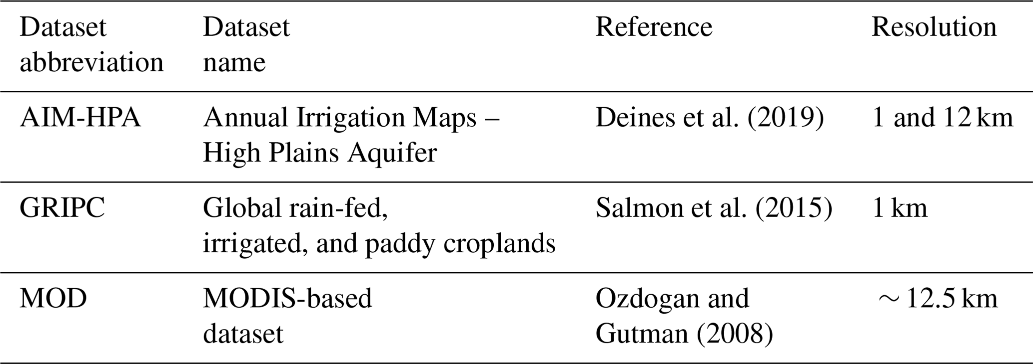
One of the first datasets to leverage machine learning applications in remote sensing used an image classification algorithm along with MODIS vegetation indices, ancillary climate, and agricultural data to map irrigated areas in the continental US circa 2001 (hereafter MOD; Ozdogan and Gutman, 2008). The resulting dataset, produced at a 500 m resolution, showed an estimated root-mean-square error (RMSE) of about 2 % of the total irrigated area in the US. Using a similar methodology, but expanding the analysis to the global scale, the “Global rain-fed, irrigated, and paddy croplands” (GRIPC; Salmon et al., 2015) map also used a machine learning algorithm applied to MODIS data, climate data, and existing information from other datasets to map not only irrigated areas but also rainfed and paddy croplands at a 500 m resolution, circa 2005. More recently, Deines et al. (2019) used Google Earth Engine to process Landsat data and environmental covariables using a random forest classifier to create the Annual Mapping of Irrigated Areas – High Plains Aquifer (AIM-HPA) dataset, consisting of one map per year from 1984 to 2017 at a 30 m resolution for the High Plains Aquifer region of the central US. The high temporal and spatial resolution of this dataset marks a major advancement in irrigation mapping that has benefits not only for weather and climate modeling but also for the management, policy, and agronomy fields (Deines et al., 2019).
This work explores the impacts of these three, high-quality and widely used irrigation datasets – MOD, GRIPC, and AIM-HPA (Table 1) – on land–atmosphere interactions in eastern Nebraska using a case study from the Great Plains Irrigation Experiment (GRAINEX) field campaign. It should be noted that the purpose of this study is not to discern the most accurate irrigation map for the study area; rather, this work is a model sensitivity study that seeks to understand if and the extent to which irrigation heterogeneity (via irrigation map selection and resolution) can impact the simulation and prediction of land–atmosphere coupling and ambient weather, and it discusses the implications of such impacts in the context of sub-grid-scale process representation in coarser-scale models.
Table 1List of irrigation maps used in the simulations, including their references and resolutions.
3.1 Models and experimental design
This study uses version 3.3 of the Noah land surface model (Chen and Dudhia, 2001) within the NASA Land Information System (LIS; Kumar et al., 2006) to complete long-term (2010–2019), land-only spin-ups of land surface states (soil moisture and temperature) and fluxes (sensible and latent). A long-term LSM spin-up that is consistent in its irrigation treatment is essential for the proper, equilibrated initialization of the subsequent coupling simulations. The modeling domain is 360 km × 360 km with a spatial resolution of 1 km and encompasses the GRAINEX field campaign study region (Fig. 1). The land-only simulations are forced with meteorological data from Phase 2 of the National Land Data Assimilation System (NLDAS-2; Xia et al., 2012) and use MODIS International Geosphere–Biosphere Program (MODIS-IGBP) land cover and National Centers for Environmental Prediction (NCEP) climatological greenness vegetation fraction (GVF) and leaf area index (LAI) datasets.
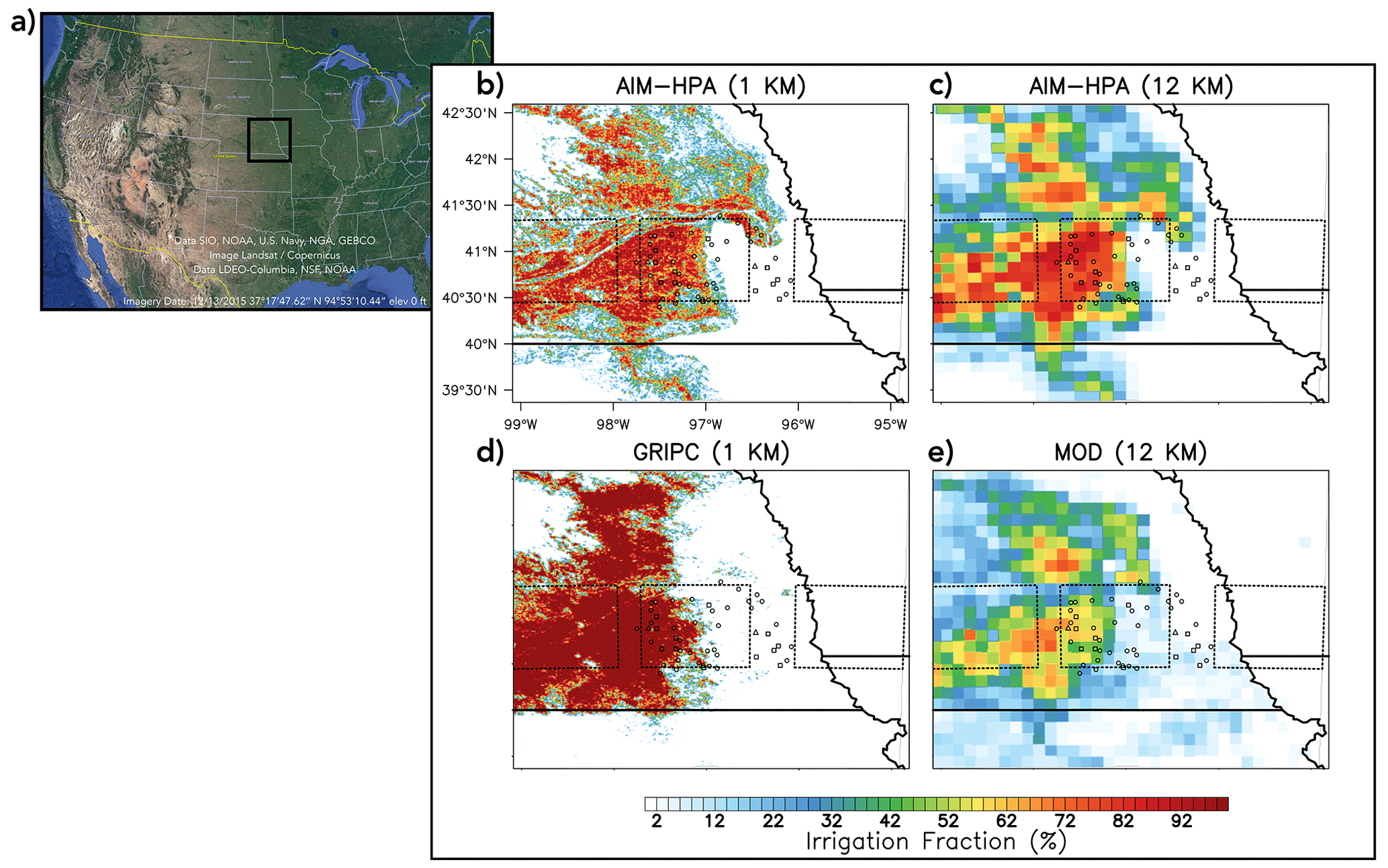
Figure 1Panel (a) presents a map of the USA (Google Earth Pro, 2023) with a box indicating the location of the study area. Panel (b) shows the application of the AIM-HPA 1 km, (c) AIM-HPA 12 km, (d) GRIPC 1 km, and (e) MOD 12 km irrigation fraction datasets to the modeling domain. Boxes show the irrigated (left), transition (middle), and rainfed (right) 100 km × 100 km domains used in the analysis shown in Figs. 4 and 5.
The irrigation parameterization within LIS/Noah is activated when four conditions are met: (1) the land cover must be an irrigable type (e.g., non-urban or bare soil land cover); (2) the irrigation fraction must be nonzero, (3) the simulation date or time must be within the “growing season”, defined by a grid cell GVF greater than 40 % of the annual range in climatological GVF; and (4) the root zone must be dry enough to require irrigation, as determined by root zone moisture availability that falls below a user-defined field capacity threshold. Ozdogan et al. (2010) determined 50 % of field capacity to be sufficient based on correspondence with local experts in Nebraska and California as well as on trial and error. Due to this previous work, as well as previous assessments of the irrigation scheme and modeling system (Lawston et al., 2017), this study also uses a threshold of 50 % of field capacity. The root zone is determined by the crop type and scaled by GVF to mimic a seasonal cycle of root growth. If all conditions are met, water will be applied as precipitation (mimicking a “sprinkler” application) until the root zone moisture availability reaches 80 % of field capacity. Center-pivot sprinklers are the most common method of irrigation in Nebraska (NASS, 2009). The irrigation fraction is used to scale the amount of water applied. More details about the irrigation schemes as well as an evaluation and sensitivity analysis of the irrigation scheme and thresholds can be found in Ozdogan et al. (2010) and Lawston et al. (2015, 2017). The irrigation scheme, thresholds, and all datasets except irrigation fraction (i.e., land cover, GVF, soil texture, crop type, and meteorological forcing) are kept constant between runs.
Three different irrigation maps, MOD, GRIPC, and AIM-HPA (see Sect. 2), are used in the land-only simulations. These datasets have a relatively high native resolution (30 m for AIM-HPA and 500 m for MOD and GRIPC) but are upscaled to the model 1 km grid at varying resolutions to discern not only the impact of differing irrigation sources but also of varying the dataset resolution. The AIM-HPA dataset for the year 2017 (the most recent year available at the time of this work) is upscaled to both 1 and 12 km, GRIPC is upscaled to 1 km, and MOD is upscaled the resolution of the NLDAS domain (∼ 12.5 km). These simulations provide the opportunity to discern the impacts of heterogeneity resulting from the following: (1) a single-dataset resolution only (i.e., AIM-HPA 1 km vs. AIM-HPA 12 km), (2) different datasets at a coarser resolution (MOD 12 km vs. AIM-HPA 12 km) and a higher resolution (i.e., GRIPC 1 km vs. AIM-HPA 1 km), and (3) using a product at an “off-the-shelf” resolution (i.e., MOD ∼ 12 km). An additional baseline run with the irrigation scheme inactive is also completed (hereafter NO IRR), resulting in five runs (i.e., NO IRR, MOD 12 km, GRIPC 1 km, AIM-HPA 1 km, and AIM-HPA 12 km).
Each land-only spin-up is used to initialize a fully coupled simulation with the NASA Unified Weather Research and Forecasting System (NU-WRF; Peters-Lidard et al., 2015), which is coupled to LIS (i.e., LIS-WRF; Kumar et al., 2008). These five LIS-WRF simulations are run for 30 h from 00:00 UTC on 24 July to 12:00 UTC on 25 July 2018. This time period was selected to build upon previous GRAINEX analyses (Rappin et al., 2021, 2022) that identified it as the most ideal period for the evaluation of irrigation's impact on L–A coupling during the second intensive observation period (IOP). The LIS-WRF simulations are forced using meteorological data from the NCEP Final Analysis (FNL; https://rda.ucar.edu/datasets/ds083.3/, last access: 10 October 2021). The model setup has 60 vertical levels and uses Mellor–Yamada–Nakanishi–Niino Level-2.5 (MYNN2.5; Nakanishi and Niino, 2006) surface layer and PBL schemes. The identical irrigation scheme, thresholds, and respective datasets used in the land-only simulations are also used in the coupled runs, ensuring continuity between the spun-up initial conditions and the coupled irrigation parameterization.
Figure 1 shows the irrigation maps applied to the modeling domain for the four irrigated runs along with markers indicating the locations of relevant GRAINEX observation sites and boxes defining subregions used in the analysis detailed in Sect. 4. There are several key differences that emerge among the maps. When comparing the higher-resolution maps (i.e., Fig. 1b vs. d), AIM-HPA extends the irrigated area further to the east and south than the GRIPC dataset and has a wider range of irrigated fraction values. More specifically, most grid cells classified as irrigated by GRIPC show a high irrigation fraction (> 90 %), whereas AIM-HPA is more heterogeneous, even in the heart of the irrigated area. Some of this heterogeneity is lost when upscaling to 12 km (Fig. 1c), but a greater range in irrigation fraction still exists compared with the other coarser-resolution run, MOD (Fig. 1e). The location of the highest-intensity irrigation in the MOD dataset is similar to the others (i.e., roughly between 97 and 98∘ W), but MOD is an outlier in that it extends a low percentage of irrigation (i.e., < 30 %) far eastward, well into what is considered to be rainfed areas of the GRAINEX study domain.
3.2 Observations
To comprehensively observe the impacts of irrigation on the atmosphere, GRAINEX (Rappin et al., 2021) deployed a collection of observation systems in a 100 km × 100 km region of eastern Nebraska in May–August 2018. This field campaign, funded by the National Science Foundation (NSF), was centered on a divide between predominately irrigated (west) and rainfed agriculture (east). Observation systems used during the campaign include 12 flux towers, 80 temporary meteorological observation stations, 2 vertical wind profilers, and regular radiosonde launches (Rappin et al., 2021). The campaign also featured two IOPs, (1) 29 May–13 June and (2) 16–30 July, in order to more rigorously observe the impacts of the commencement and peak of irrigation, respectively. Analysis of the GRAINEX data has shown that air temperature, wind speed, and the planetary boundary layer height (PBLH) were lower over the irrigated area compared with the nonirrigated region (Rappin et al., 2021, 2022) and that irrigation in the upslope region of the domain weakened terrain-induced baroclinicity and the slope wind circulation (Phillips et al., 2022).
Observations from the GRAINEX field campaign are used to assess the model simulations. Figure 2 shows the locations of the comprehensive land and PBL profiling instruments used in this study overlaid on the irrigation fraction given by the AIM-HPA dataset. The green, orange, and red circles in Fig. 2 note the locations of 38 Environmental Monitoring Economical Sensor Hub (EMESH) meteorological stations. EMESH weather stations were developed at the University of Alabama in Huntsville and were field tested for accuracy and reliability. Each EMESH station recorded standard meteorological data, such as air temperature, barometric pressure, relative humidity, wind speed and direction, and rainfall, as well as soil moisture and temperature. The blue triangles in Fig. 2 indicate the locations of two Integrated Sounding System (ISS) sites. The western ISS site (i.e., York) is surrounded by irrigated agriculture, whereas the eastern site (i.e., Rogers Farm) is representative of the nonirrigated region. Instrumentation at each ISS site included a ceilometer, radar wind profiler, weather station, and 2-hourly radiosonde launches from sunrise (∼ 11:00 UTC) to sunset (∼ 01:00 UTC). In this study, we use weather data (e.g., temperature, humidity, and pressure) from the EMESH stations (Nair et al., 2019) and radiosonde observations from the Rogers Farm (UCAR/NCAR, 2018a) and York ISS sites (UCAR/NCAR, 2018b). More information about the EMESH stations and the ISS sites as well as a full description of all instruments deployed during the campaign can be found in Rappin et al. (2021).
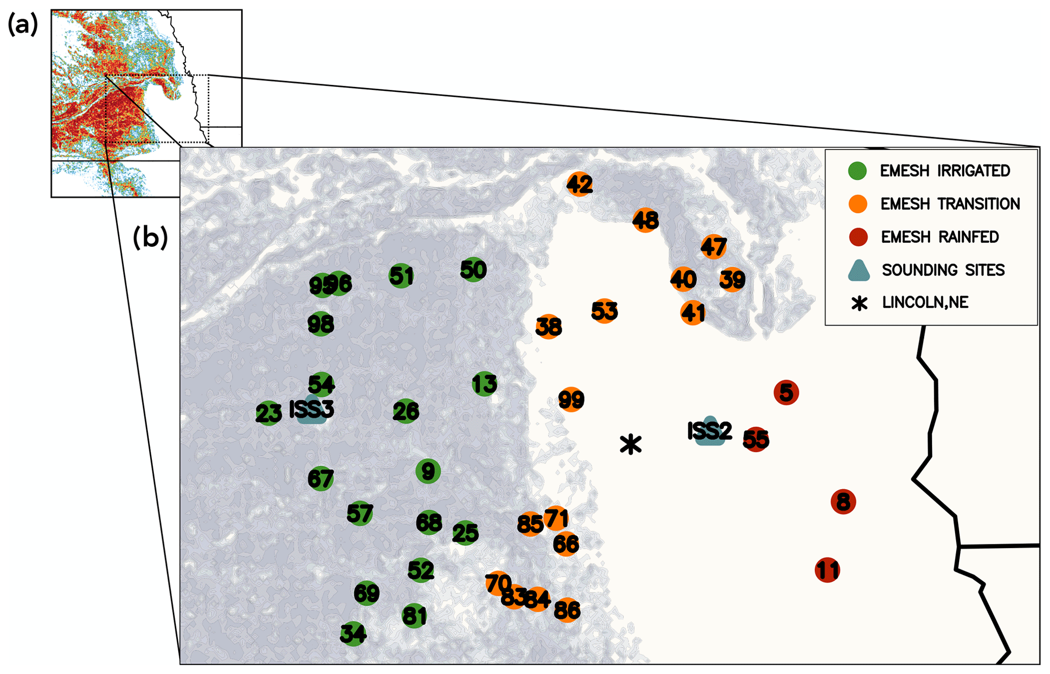
Figure 2(a) The AIM-HPA 1 km irrigation dataset applied to the modeling domain with a box noting the zoomed in area in panel (b). (b) Locations of the GRAINEX instruments overlaid on the AIM-HPA 1 km irrigation fraction dataset. Circles indicate stations with meteorological observations (i.e., temperature and humidity), classified as irrigated (green), transition (orange), and rainfed (red). Blue triangles are the locations of radiosonde launches (i.e., ISS sites) at the irrigated (ISS3 – York) and nonirrigated (ISS2 – Rogers Farm) sites.
In order to investigate the irrigation dataset heterogeneity impacts in different subregions of the domain, the EMESH stations are classified as being in irrigated (green circles), transition (orange circles), or rainfed (red circles) regions. EMESH stations with a longitude less than (i.e., west of) 97.084∘ W are well within the irrigated area and are classified as “irrigated” stations, whereas those with a longitude greater than (i.e., east of) 96.335∘ W are classified as rainfed stations. The stations located between 97.084 and 96.335∘ W are classified as transition stations, as they are likely subject to both irrigated and nonirrigated effects under typical synoptic conditions. These longitude cutoffs were chosen to encompass both the boundary of irrigation given by the AIM-HPA 1 km map and the Big Blue River, the latter of which is locally understood to be the unofficial “dividing line” between predominately irrigated and rainfed agriculture (Rappin et al., 2021). In addition, a coarser-scale subregional analysis is completed that imposes three 100 km × 100 km boxes on the study region (shown in Fig. 1), as proxies for three ESM grid cells that are mostly irrigated, partially irrigated (i.e., transition), and mostly rainfed (as discussed in Sect. 4).
3.3 Land–atmosphere (L–A) interactions
The local L–A coupling (i.e., LoCo; Santanello et al., 2018) process chain paradigm provides an integrative framework for assessing the impacts of land surface heterogeneity (LSH) by evaluating the relative sensitivities of (1) surface fluxes to soil moisture; (2) PBL evolution to fluxes; (3) entrainment fluxes to PBL evolution; and (4) the collective feedback of the atmosphere on ambient weather, clouds, and precipitation. This allows for a more comprehensive analysis of the coupling impacts of heterogeneity vs. a traditional one-at-a-time approach (e.g., evaluating evapotranspiration or air temperature independently). In this study, the complete set of process chain variables are not available at any individual site, so we do not undertake a site-by-site, end-to-end LoCo assessment. Rather, we use the process chain framework to assess the bulk land surface forcing by using aggregates of observations and models across regions. In particular, we employ (1) evaporative fraction (EF = latent heat flux/latent heat flux + sensible heat flux) vs. PBL height (PBLH) plots and (2) a modified version of mixing diagrams (Santanello et al., 2009, 2018). Traditional mixing diagrams relate the diurnal coevolution of temperature and moisture in the boundary layer using vectors representing the surface input of heat and moisture scaled by the PBLH. As surface fluxes and PBLH observations are not co-located with near-surface meteorology observations, the vectors are excluded from this analysis.
Figure 3 shows the differences between no irrigation and each irrigation simulation in top-layer soil moisture, EF, temperature at 20 m, humidity (mixing ratio) at 20 m, and the PBLH, along with the GRAINEX instrument locations for reference. The 20 m model height (rather than 2 m) is chosen throughout the analysis to assess the bulk (ambient) signal of irrigation, as 2 m values will be more reflective of hyper-local vegetation and crop characteristics and irrigation practices in the field. In each case, irrigation increases soil moisture, latent heat flux, and near-surface humidity, as expected, with a corresponding decrease in sensible heat flux, temperature, and the PBLH. The spatial pattern of changes in soil moisture and evaporative fraction corresponds closely to the irrigation data source, as the irrigation map determines the location of soil moisture increases, which then directly affect fluxes via the terrestrial leg of the L–A coupling chain (Dirmeyer, 2011). The impacts on the PBLH and temperature and humidity are more representative of the bulk atmospheric integrated (spatially and vertically) response to irrigation (i.e., the atmospheric leg of L–A coupling), and, as such, the impacts extend a bit beyond the actual boundaries of irrigated area, particularly in the southern region as the result of light northerly winds.
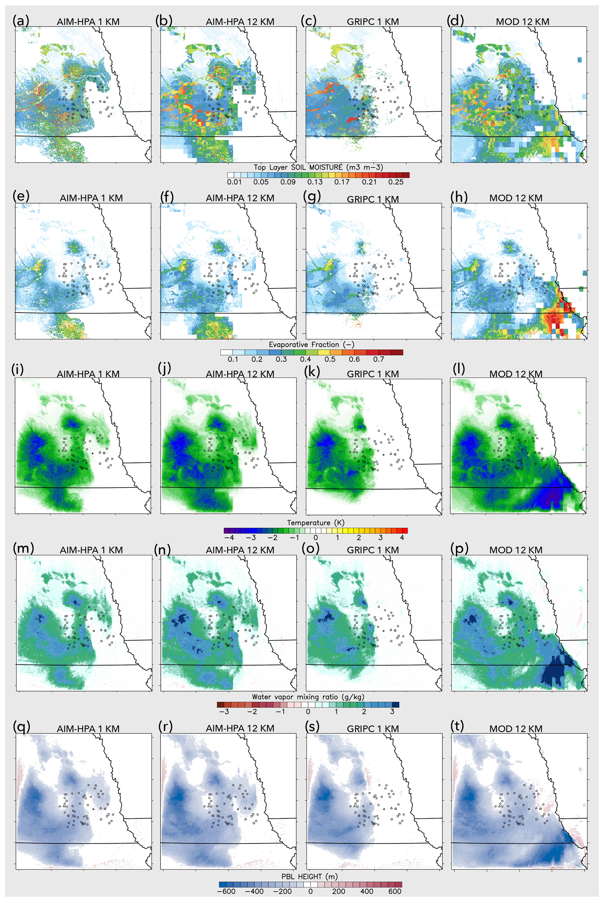
Figure 3Difference from the control as a daytime average for the (a–d) top-layer soil moisture, (e–h) evaporative fraction, (i–l) temperature at 20 m, (m–p) humidity (mixing ratio) at 20 m, and (q–t) PBLH for the AIM-HPA 1 km, AIM-HPA 12 km, GRIPC 1 km, and MOD 12 km runs.
The spatial extent and magnitude of irrigation-induced changes vary based on the selected irrigation map, with the biggest differences stemming from the dataset source, rather than the resolution. The MOD map is the clear outlier, as the irrigated area and subsequent impacts extend well east into the actual rainfed region of the GRAINEX domain. The biggest changes are observed in the southeast corner of the domain, where even a small amount of irrigation fraction (4 %–16 %) increases soil moisture by 0.1–0.15 m3 m−3 and reduces temperature by up to 3 K. The GRIPC map most closely matches the GRAINEX site-level classification of irrigated and rainfed sites, largely bisecting the site locations and limiting most impacts to Nebraska, whereas the other irrigation maps extend south into Kansas. The AIM-HPA maps at different resolutions are quite similar, but the upscaling limits the precision of the spatial heterogeneity at the irrigated vs. nonirrigated border as well as the subsequent impacts.
In order to analyze the extent to which essential L–A coupling information, driven by the irrigation heterogeneity, is retained at the ESM scale, three 100 km × 100 km subregions are imposed on the study domain, indicated by the boxes in Fig. 1. The western subregion is largely irrigated, the center contains the transition area from irrigated to rainfed, and the eastern is predominantly rainfed. These subregions can be viewed as a proxy for an ESM grid cell, with the model 1 km grid cells contained within them serving as “tiles” in which the ESM sub-grid L–A processes are fully resolved.
Figure 4 presents plots of the daytime average EF vs. the maximum PBLH, which is a critical coupling metric that relates the daytime surface flux of heat and moisture (i.e., the land forcing) to the PBL response (Santanello et al., 2009, 2011). The gray circles represent the EF and PBLH (given as the model diagnostic from the MYNN scheme) values for each 1 km grid cell within the irrigated subregion for each model run. The colored markers show the subregional average for each model run and are, therefore, the same for each figure panel (Fig. 4a–e). The NO IRR run (Fig. 4a) shows the variability in the EF and PBLH that results from natural heterogeneity in the model (e.g., land cover and soil type) and reveals that this subregion is fairly wet on this day even without irrigation, as most grid cells have EF values of 0.5 or greater. In the irrigated runs (Fig. 4b–e), the irrigation scheme increases the EF in most grid cells and greatly reduces the PBLH compared with NO IRR. Although the spatial averages are very similar across the irrigated runs (e.g., colored markers grouped near an EF of 0.8 and PBLH of 1100 m), the spread across the 1 km tiles varies considerably. For example, the AIM-HPA 1 km dataset produces the most spatial variability in the EF (i.e., numerous points spread between an EF of 0.3 and 0.7 across the 100 km box), due to the local heterogeneity that extends to lower and, importantly, zero irrigation fraction values. This variability in EF is lost when upscaling to 12 km (Fig. 4c). In fact, AIM-HPA 12 km more closely resembles the MOD 12 km run (Fig. 4d), which has a positive irrigation fraction throughout the region, than the AIM-HPA 1 km run, suggesting that resolution of the irrigation fraction dataset can play a key role in the terrestrial leg of L–A coupling. Despite the lower EF values seen in this subregion in the AIM-HPA and GRIPC runs, there is little impact on the PBL growth, likely due to the bulk of the domain being irrigated and the spatial and vertical blending of that influence.
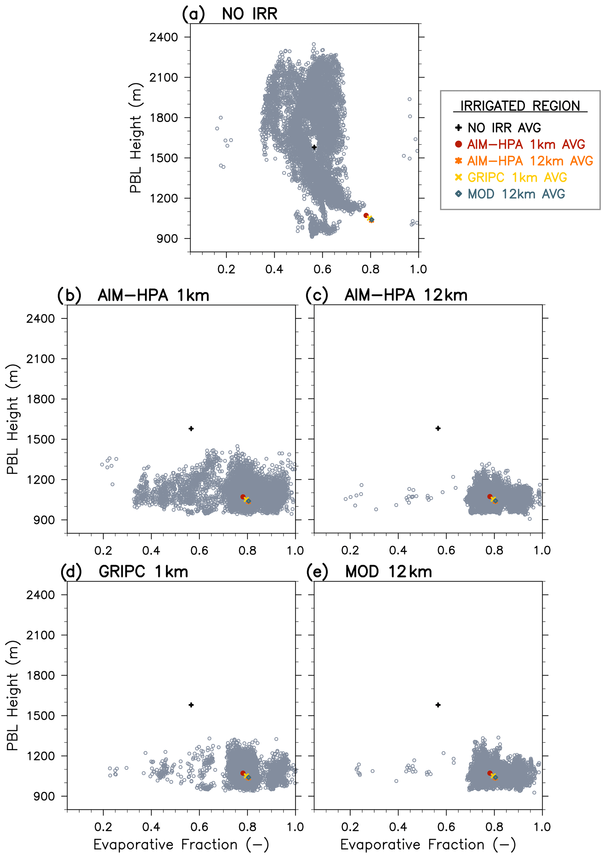
Figure 4Evaporative fraction vs. PBLH plots for the irrigated subregion for the (a) NO IRR, (b) AIM-HPA 1 km, (c) AIM-HPA 12 km, (d) GRIPC 1 km, and (e) MOD 12 km runs. There is one gray marker for each 1 km grid cell within the 100 × 100 km irrigated subregion. The colored markers represent the subregional average for each run and are, therefore, the same for each subplot.
Figure 5 shows the EF vs. PBLH plots for the transition region for all runs. The NO IRR run (Fig. 5a) shows tight grouping of points with fairly clean borders governed by the natural heterogeneity (e.g., land cover, soil type, and vegetation characteristics) and associated model thresholds and parameters. The irrigated runs (Fig. 5b–e) show how irrigation and the irrigation fraction map itself change the heterogeneity in the EF vs. PBLH. For example, in the transition region, the MOD run extends irrigation to the east such that the transition region is almost entirely irrigated, resulting in EF values that are skewed towards the high (i.e., wet) end of the EF, whereas two clusters (wet vs. moderate) emerge as a result of the precisely resolved irrigation boundary in the AIM-HPA 1 km run. Notably, the wetter cluster in the AIM-HPA 1 km run has EF values similar to the MOD run (i.e., ∼ 0.65–0.9) but has corresponding PBLH values that are up to 400 m higher than in MOD. It is likely that the drier (east of the AIM-HPA transition boundary) grid cells that have higher sensible and lower latent heat impact larger PBL growth and entrainment feedbacks (as the PBL can integrate over 10–50 km horizontally; Stull, 1988), and the influence is felt beyond just the nonirrigated region. This implies that some grid cells in the AIM-HPA 1 km run (but not MOD, which has irrigation throughout) reach critical moisture and PBL thresholds that allow for PBL feedbacks that increase the height of the PBL. The L–A interactions that lead to these feedbacks are a direct result of the irrigation map and triggering thresholds and, in turn, could be important for cloud development and convective processes in a sub-grid ESM parameterization.
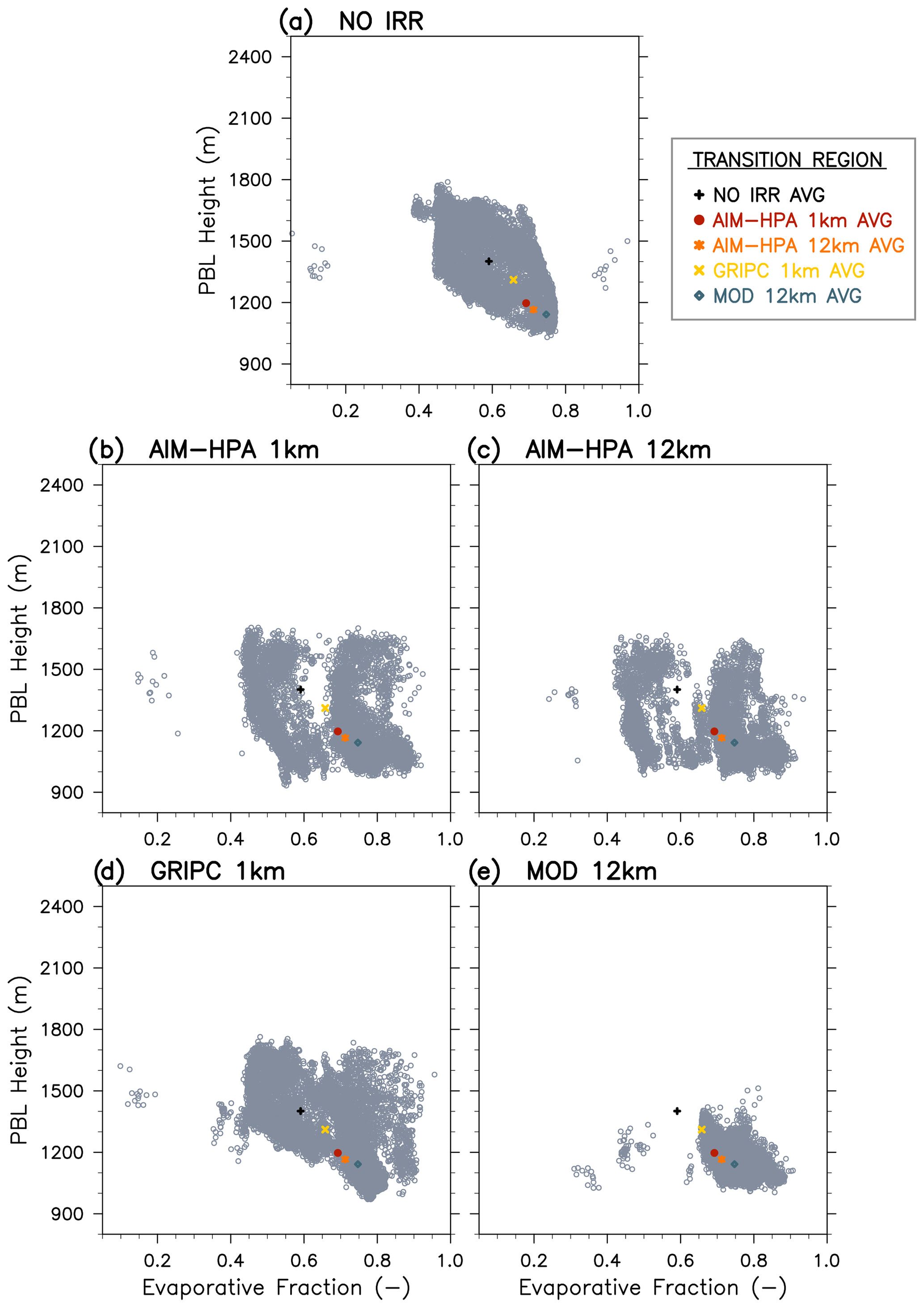
The rainfed region (Fig. S1 in the Supplement) shows considerable spread in both the EF and PBLH but little difference across runs, as all datasets specify a zero or near-zero irrigation fraction. This allows “natural” heterogeneity in the EF to dominate, which is dependent on land cover, soil type, terrain, and precipitation. Overall, it is clear from the intercomparison of the three subregions that irrigation (and choice of dataset in coupled models) can be a dominant and/or limiting (Fig. 4), conditional (dependent on the orientation of the fraction map, boundaries, and wind flow; Fig. 5), or minimal (i.e., natural heterogeneity dominates; Fig. S1) control on L–A coupling and the processes that govern the relationship of soil moisture, fluxes, and PBL growth on ambient weather.
Figure 6 presents mixing diagrams for seven subregions of the GRAINEX domain. All irrigation maps define the western part of the domain as heavily irrigated, but the maps differ considerably in their representation of the heterogeneity within the irrigated area and in defining the location and characteristics of the transition between irrigated and rainfed areas. To address this within-region heterogeneity, the EMESH sites are classified into the following seven subregions using the AIM-HPA 1 km irrigation map: North Irrigated, Middle Irrigated, and South Irrigated (Fig. 2, green circles); Northeast Transition, Northwest Transition, and Southwest Transition (Fig. 2, orange circles); and Rainfed (Fig. 2, red circles). Table 2 lists the specific site numbers included in each subregion.
Table 2List of GRAINEX EMESH sites, including the subregional classification used in Fig. 6, and the irrigation fraction given by each dataset for the grid cell closest to the site's latitude and longitude.
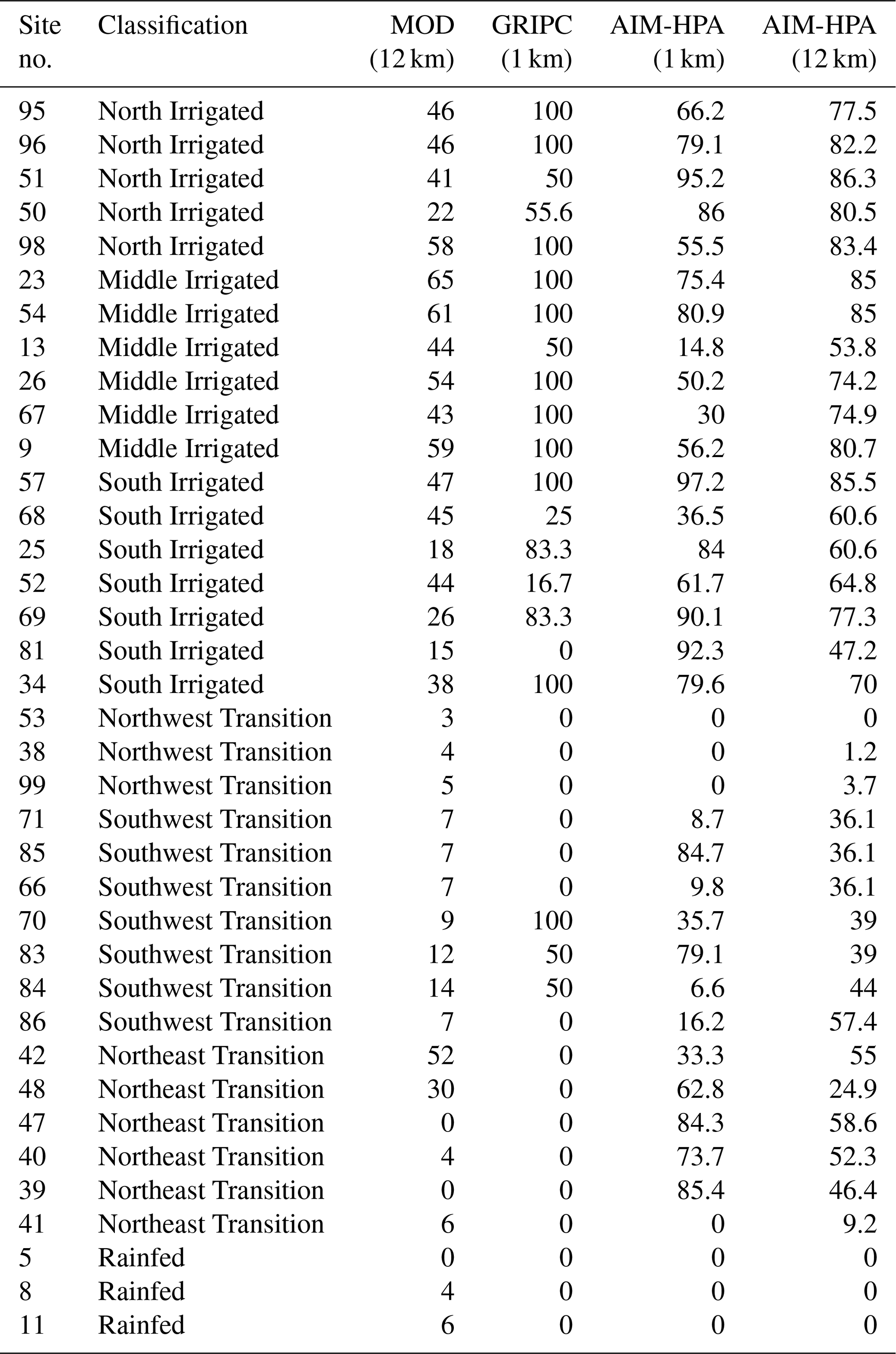
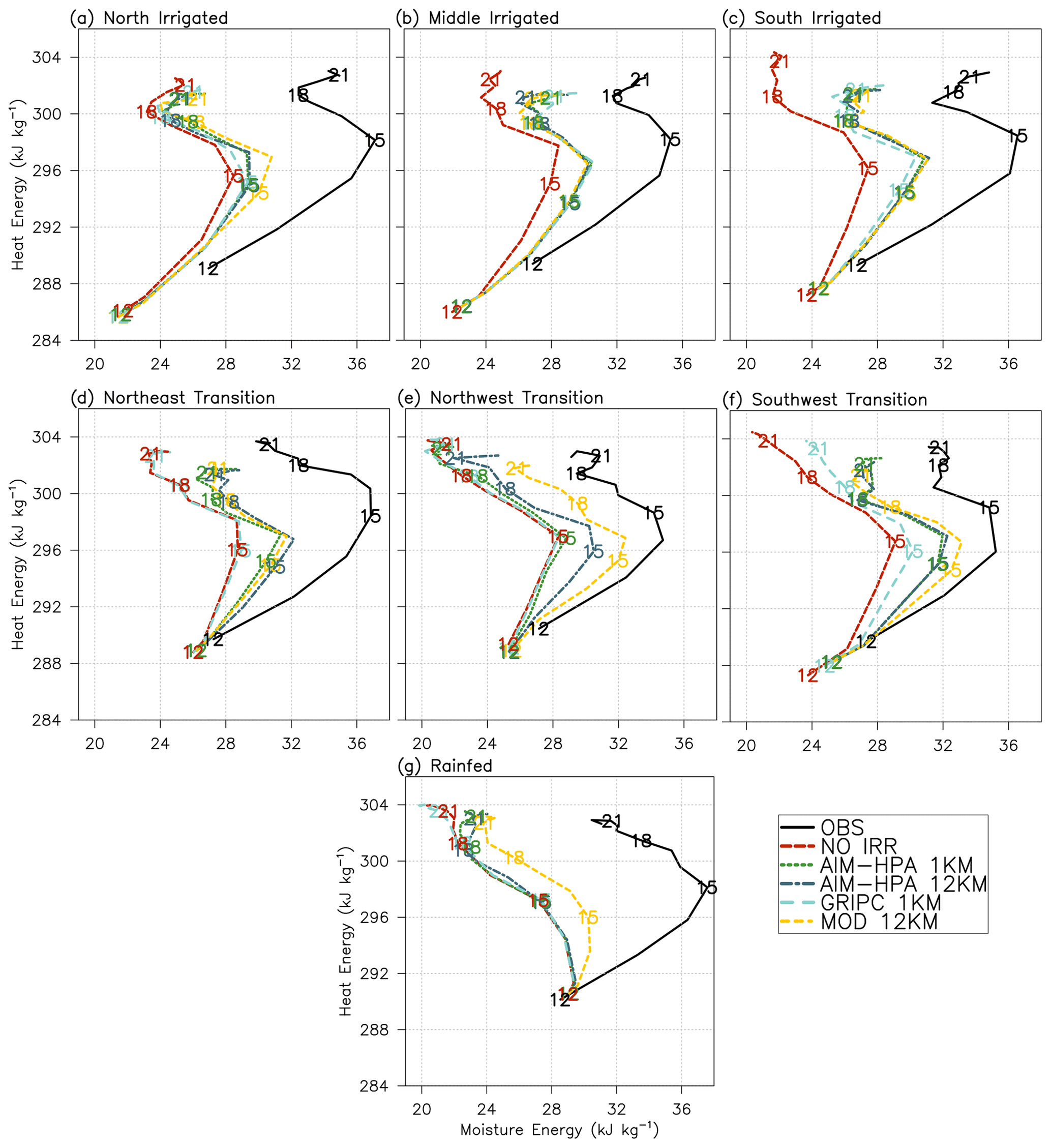
Figure 6Average mixing diagrams for the (a) North Irrigated, (b) Middle Irrigated, (c) South Irrigated, (d) Northeast Transition, (e) Northwest Transition, (f) Southwest Transition, and (d) Rainfed subregions.
Figure 6 shows that there is tight grouping across (i.e., minimal difference in) the irrigation runs in the Middle Irrigated (Fig. 6b) and South Irrigated (Fig. 6c) regions. Irrigation can affect the simulations through (1) wetter initial soil moisture conditions from the irrigated spin-up (i.e., previous irrigation) and (2) irrigation in the coupled simulation (i.e., present irrigation). The similar performance displayed by the irrigation runs is due to the combined facts that (1) there is agreement among the maps that these regions are heavily irrigated and (2) these regions also exhibit low antecedent moisture (Fig. S2), causing irrigation to turn on in the coupled run. In contrast, the North Irrigated (Fig. 6a) region, while also heavily irrigated, has wetter antecedent soil moisture, so irrigation does not turn on in the coupled run at the sites that make up this region. Rather, the spread is due to previously applied irrigation from which the model has begun to dry out.
The irrigation maps differ the most in the transition region between irrigated and rainfed, leading to the greatest spread in model runs in the Northwest Transition (Fig. 6e) and Southwest Transition (Fig. 6f) subregions. In the Rainfed (Fig. 6g) subregion, the MOD run is the outlier as it classifies the rainfed sites as irrigated, whereas all other runs are close to the NO IRR run because they correctly classify these sites as rainfed. Figure 6 also shows that the model has an inherent dry bias, as the observations are consistently more humid than the NO IRR run in all subregions, including Rainfed. The irrigation scheme, regardless of the prescribed irrigation fraction map, acts to mitigate this bias, compensating for other model errors beyond only the lack of irrigation in the model.
In order to better understand the irrigation impacts on the PBL, the York (irrigated) and Rogers Farm (rainfed) sites are analyzed in more detail in Figs. 7, 8, and 9. Figure 7 again shows mixing diagrams, although this time for the single sites (i.e., not spatial averages as in Fig. 6) of York and Rogers Farm, using temperature and humidity at 20 m in the model and at the level closest to 20 m from radiosonde observations. At the York site, the model starts the day considerably cooler and drier than observations, but the daytime heating vigorously warms and moistens the boundary layer, bringing all model runs closer to observations by late morning (e.g., 15:00 UTC). The model follows the diurnal cycle of the observations well, implying that it captures the warming and moistening of the boundary layer early in the day, the subsequent drying due to entrainment around midday (i.e., the “left turn” in the diagram), and the second round of moistening late in the day (i.e., the final “right turn”).
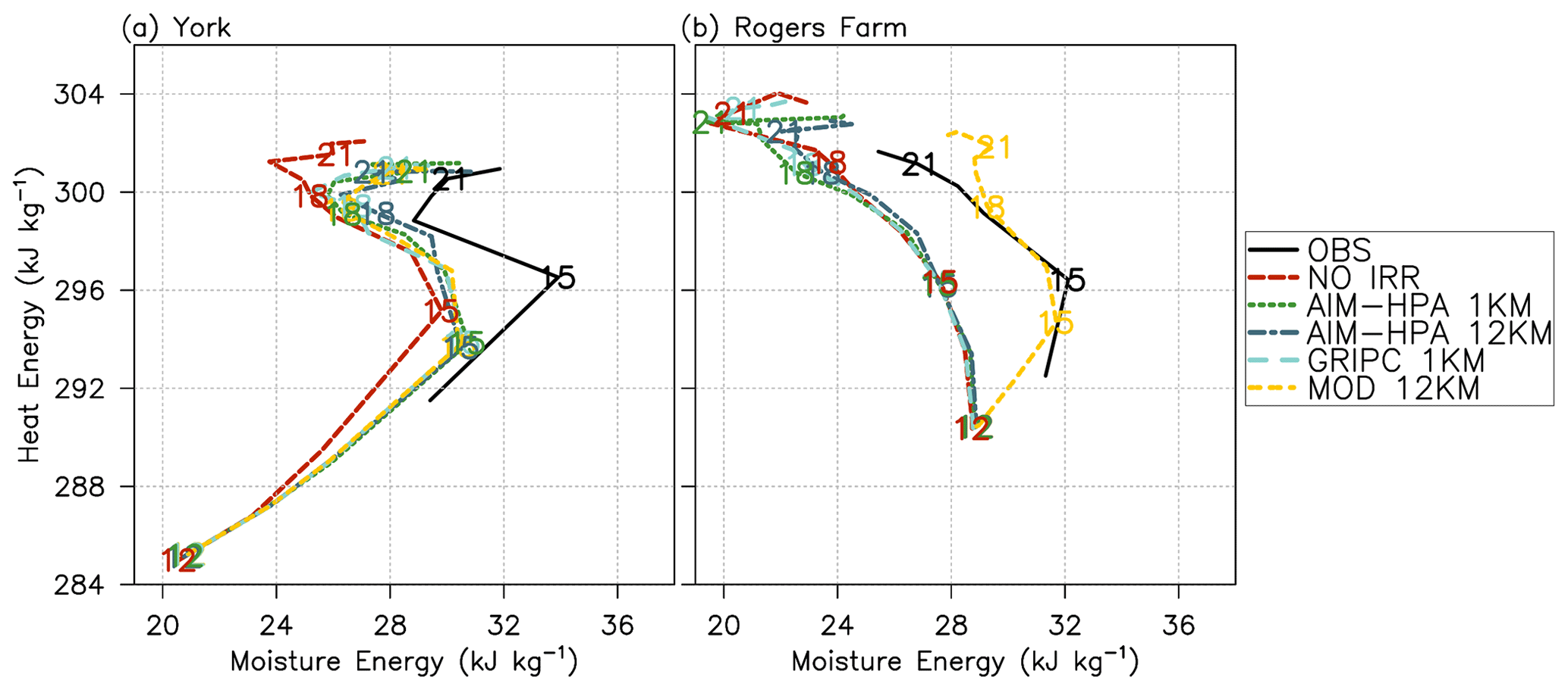
Figure 7Mixing diagrams for the (a) York (ISS3 – irrigated) and (b) Rogers Farm (ISS2 – rainfed) Integrated Sounding System sites.
At the Rogers Farm site, most of the model runs capture the midday drying well (slow leftward curve) but miss the small morning moistening from 13:00 to 15:00 UTC shown in observations. In addition, the models display a late day moistening (20:00–23:00 UTC or 15:00–18:00 LT, local time) that does not appear in observations. The exception is the MOD run, which shows the moistening early in the day and gradual drying throughout the day, more consistent with observations. The better performance of MOD is due to misclassifying this site as a small percentage irrigated and, therefore, mitigating the existing dry bias in the model.
Figures 8 and 9 show 2-hourly (15:00 UTC on 24 July to 01:00 UTC on 25 July) potential temperature profiles for the lowest 1.8 km at the York and Rogers Farm sites, respectively. A detailed analysis of the radiosonde profiles is available in Rappin et al. (2021). Here, we focus on the differences in the model runs and their ability to simulate what was observed. At the York site, the observations show more rapid PBL growth from 15:00 to 17:00 UTC than the model as the PBL grows into a more unstable free atmosphere layer. Although the model is slower in simulating this growth at 17:00 UTC, the well-mixed layer and the PBLH (i.e., approximated as the level corresponding to the maximum gradient in potential temperature) are remarkably well simulated during 19:00–23:00 UTC. The NO IRR simulation is the outlier, as it simulates a warmer boundary layer throughout the diurnal period. Little difference is noted between the irrigated runs at this site.
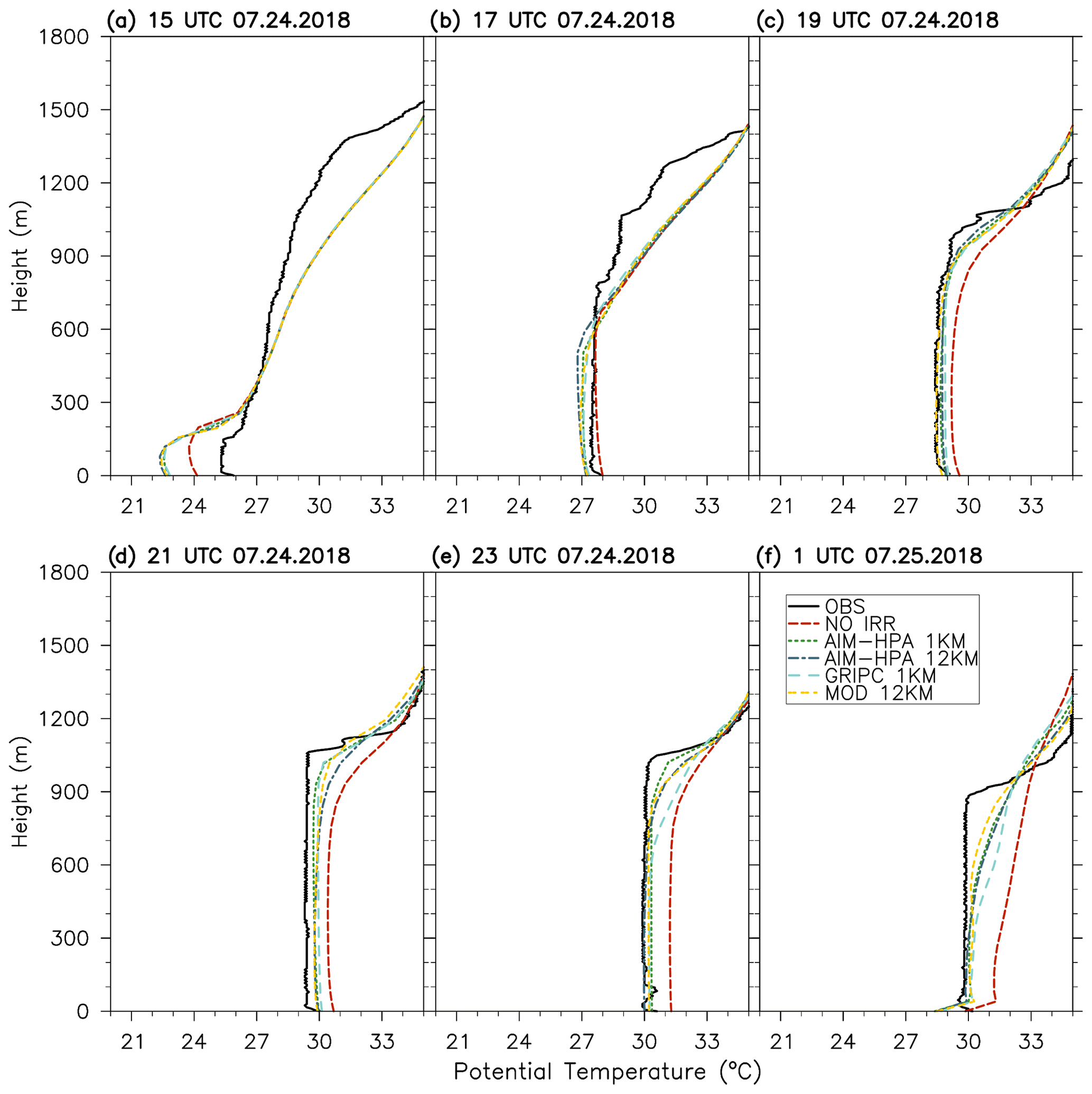
Figure 8Potential temperature profiles for each model run and observations at the York Integrated Sounding System site (ISS3 – irrigated) every 2 h from 15:00 UTC on 24 July to 01:00 UTC on 25 July.
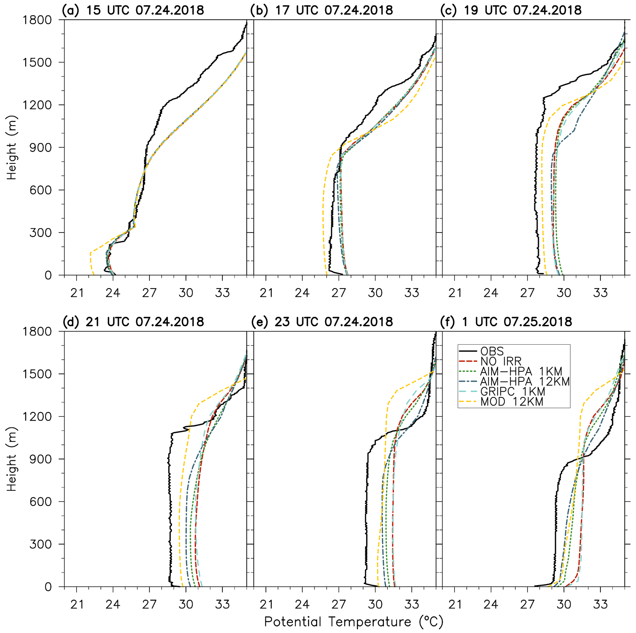
Figure 9As in Fig. 8 but for the Rogers Farm Integrated Sounding System site (ISS2 – rainfed).
At the rainfed site (Fig. 9), the model runs show a warm bias in the potential temperature profiles. The OBS (observations, black solid line in Fig. 9) are again more unstable in the free atmosphere and feature a residual layer extending to about 1300 m at 15:00 UTC. The observed PBL grows quickly to the top of the residual layer, and the PBLH reaches a maximum of about 1400 m at 19:00 UTC. The model simulates a shallower residual layer (about 900 m at 15:00 UTC) and slower growth once the PBL surpasses the top of the residual layer and grows into the more stable air in the free atmosphere. Thus, these plots illustrate that the residual layer can be a good predictor of future PBL growth (e.g., Santanello et al., 2005) and that surface changes induced by irrigation need to be considered holistically, as the PBL and lower troposphere are important modulators of the response. Figure 9 also shows more sensitivity to the irrigation fraction map (i.e., spread among runs) at the Rogers Farm site compared with York, despite irrigation not occurring at this site, except in the misclassified MOD.
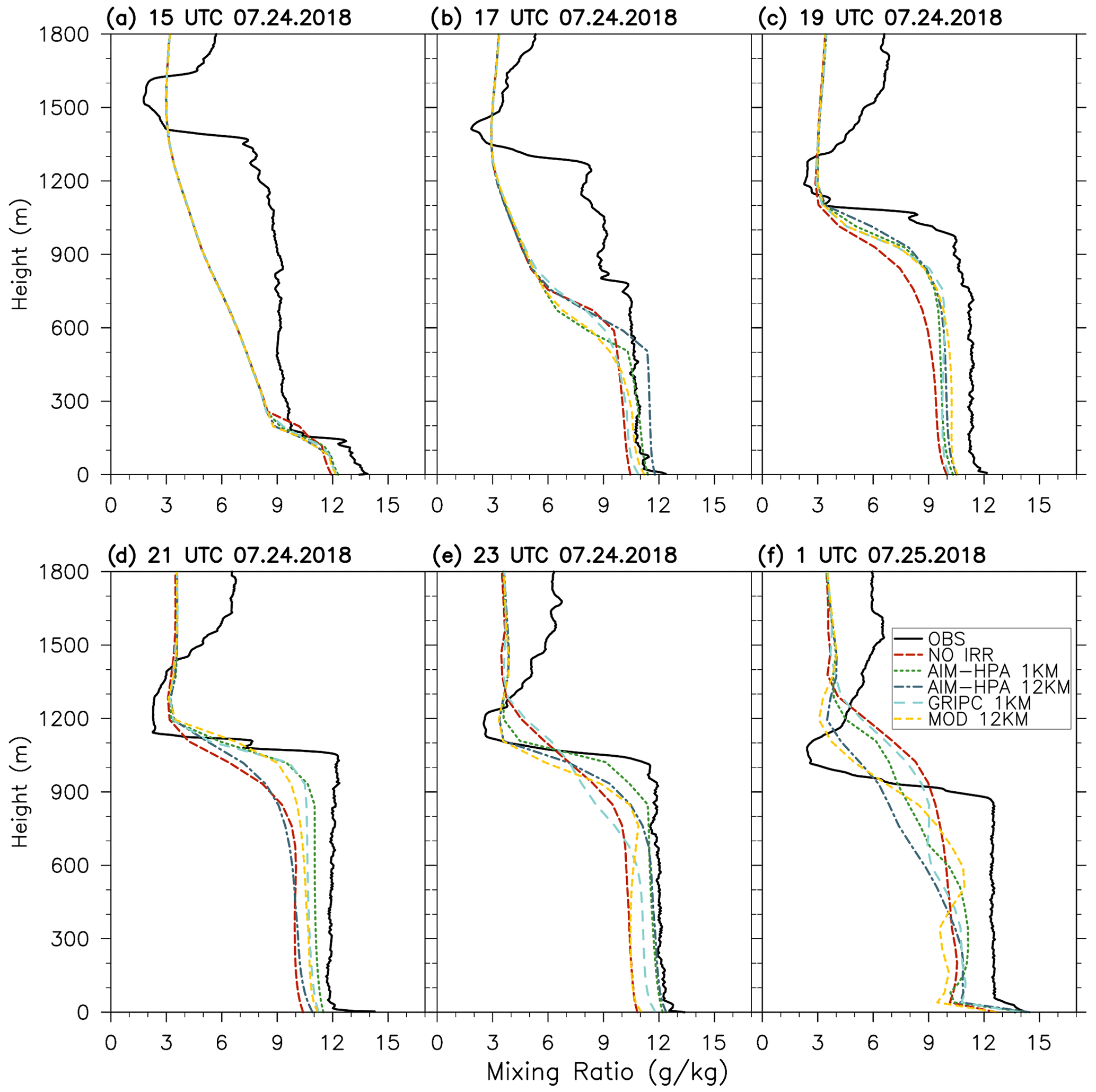
Figure 10Water vapor mixing ratio profiles for each model run and observations at the York Integrated Sounding System site (ISS3 – irrigated) every 2 h from 15:00 UTC on 24 July to 01:00 UTC on 25 July.
Figures 10 and 11 show water vapor mixing ratio profiles for the York and Rogers farm sites, respectively. At the York site, the model again exhibits a dry bias that irrigation acts to erode as it moves the irrigation runs slightly closer to observations. There is little difference between the runs early in the day. While the AIM-HPA runs at each resolution perform marginally better by 21:00 and 23:00 UTC, all of the runs perform quite well. The observations at both sites show a dry layer around 1500 m that gradually lowers throughout the day. At the rainfed site (Fig. 11), the MOD run, which exhibits greater moisture from the irrigation misclassification, lacks this dry layer, resulting in a wetter and taller boundary layer that stands out from the other runs. Overall, the models struggle to simulate the details of the elevated dry slot, with the MOD run being an outlier as a result of the irrigation misclassification.
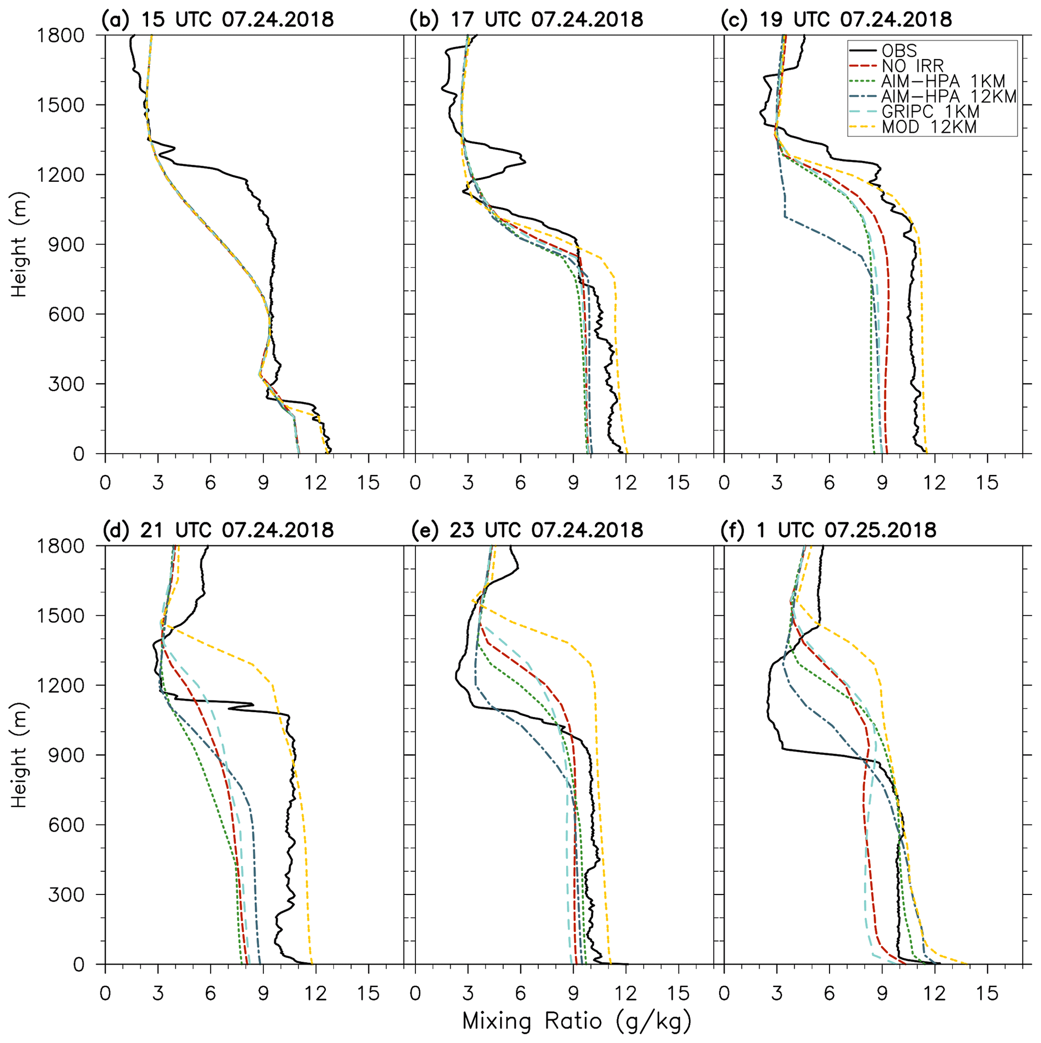
Figure 11As in Fig. 10 but for the Rogers Farm Integrated Sounding System site (ISS2 – rainfed).
This study employed a high-resolution, regional coupled modeling system to assess the impacts of the spatial representation of irrigation on L–A coupling using a case study from the GRAINEX field campaign. The simulations are assessed in the context of irrigated vs. nonirrigated regions, subregions across the irrigation gradient, and sub-grid-scale process representation in coarser-scale models.
The results show that L–A coupling is sensitive to the choice of irrigation dataset and resolution and that the irrigation impact on surface fluxes and near-surface meteorology can be dominant, conditioned on the details of the irrigation map (e.g., boundaries and heterogeneity), or minimal. For example, within the irrigated region, the irrigation map resolution had a larger influence on the spatial heterogeneity of the evaporative fraction than the choice of dataset, whereas the opposite is true (i.e., the dataset was more important) in the transition region. When viewing the simulations presented here as a proxy for “ideal” tiling in an ESM-scale grid box, the results show that some tiles will reach critical nonlinear moisture and PBL thresholds that could be important for clouds and convection, implying that heterogeneity resulting from irrigation should be taken into consideration in new sub-grid L–A exchange parameterizations, such as those being investigated within the CLASP project.
A consistent finding across several analyses was that even a low percentage of irrigation fraction can have significant local and downstream atmospheric impacts, suggesting that representation of boundaries and heterogeneous areas within irrigated regions is particularly important for the modeling of irrigation impacts on the atmosphere. In addition, the analysis of modeled and observed temperature and moisture profiles demonstrated that lower troposphere stability is an important modulator of the irrigation signal. The results also show that irrigation, regardless of the dataset, acts to mitigate an existing dry bias in the model, as highlighted by irrigation improving the bias in rainfed areas misclassified by the irrigation datasets. This underscores that care must be taken in the implementation of irrigation physics in models in order to avoid utilizing the irrigation scheme as a tuning mechanism to compensate for embedded model errors. Approaching the evaluation of irrigation schemes through a holistic L–A coupling framework, as demonstrated here, can aid in disentangling model improvements that result from new irrigation inclusion vs. the mitigation of unrelated model biases.
This study focused on a major type of human-induced land heterogeneity (i.e., irrigation) that can be introduced by model parameters and datasets, distinct from natural sources such as LULC, soil properties (e.g., type and texture), and the greenness vegetation fraction. Our results suggest that the combination of the irrigation fraction specification and the triggering algorithm creates a new type of soil moisture heterogeneity that is different from what would occur due to atmospheric forcing alone and that results in changes to L–A coupling and ambient weather.
The selected case study was chosen to fully leverage the available GRAINEX data on a favorable day for L–A interactions during IOP2 (i.e., the height of irrigation) and to build on previous GRAINEX and L–A coupling work (Rappin et al., 2021, 2022). The model antecedent soil moisture in the irrigated region ranged from 0.14 to 0.24 m3 m−3, as some regions of the domain were wet from antecedent rainfall. In addition, only one type of LSM irrigation scheme and thresholds are used in this study, whereas previous work has shown that L–A coupling is sensitive to irrigation type and factors such as vegetation greenness (Lawston et al., 2015). This enabled a controlled study on the impacts of the specific irrigation map applied, which is often overlooked in irrigation modeling impact studies (similar to land cover or soil-type datasets). A combination of mapping, thresholds, and antecedent soil moisture regime (which influences triggering) determines the irrigation heterogeneity, and these factors deserve further investigation under a wider range of atmospheric conditions. In addition, this analysis concentrated on the region of GRAINEX observations, where there are other areas of the domain with larger differences between datasets (e.g., the southeast corner) that could be explored more directly.
This work featured only three of several widely used irrigation datasets, and it is likely that the amount and variety of irrigation datasets will increase in coming years. The results of this study suggest that, to be most beneficial for irrigation representation within ESMs, future irrigation fraction datasets should ideally be high resolution, resolve large-scale irrigation boundaries, and capture within-region irrigation heterogeneity. While not investigated here, a focus of future work should be to discern the importance of the location and intensity of irrigation map boundaries on local wind and mesoscale circulations as well as the prevailing wind influences across these boundaries.
NASA's Land Information System code is open source and available on GitHub (https://github.com/NASA-LIS/LISF, Kumar et al., 2006). Data from the GRAINEX field campaign are accessible via https://doi.org/10.26023/ZEP0-XK4N-AW01 (Nair et al., 2019), https://doi.org/10.5065/D6WH2NV0 (UCAR/NCAR, 2018a) and https://doi.org/10.5065/D6RR1X4P (UCAR/NCAR, 2018b). The NASA Unified WRF code and model results are archived and can be made available from the corresponding author upon request.
The supplement related to this article is available online at: https://doi.org/10.5194/hess-27-2787-2023-supplement.
PLP and JAS Jr. formulated the experimental design. PLP completed the experiments and analyzed the simulation results and field campaign data. JAS Jr. and NWC aided PLP in the interpretation of the results and outlined their implications. PLP prepared the manuscript with contributions from all co-authors.
The contact author has declared that none of the authors has any competing interests.
Publisher’s note: Copernicus Publications remains neutral with regard to jurisdictional claims in published maps and institutional affiliations.
This work was supported by the NOAA Climate Process Teams – Translating Land Process Understanding to Improve Climate Models program. Additional funding was provided by NASA Headquarters and David Considine. Funding for GRAINEX science and airborne measurements was provided by NASA Headquarters and Jared Entin. Resources supporting this work were provided by the NASA High-End Computing (HEC) program through the NASA Center for Climate Simulation (NCCS) at Goddard Space Flight Center.
This research has been supported by the National Oceanic and Atmospheric Administration (grant no. NOAA-OAR-CPO-2019-2005530).
This paper was edited by Xing Yuan and reviewed by two anonymous referees.
Aegerter, C., Wang, J., Ge, C., Irmak, S., Oglesby, R., Wardlow, B., Yang, H., You, J., and Shulski, M.: Mesoscale Modeling of the Meteorological Impacts of Irrigation during the 2012 Central Plains Drought, J. Appl. Meteorol. Clim., 56, 1259–1283, https://journals.ametsoc.org/view/journals/apme/56/5/jamc-d-16-0292.1.xml, 2017.
Brown, J. F. and Pervez, M. S.: Merging remote sensing data and national agricultural statistics to model change in irrigated agriculture, Agr. Syst., 127, 28–40, 2014.
Biggs, T. W., Thenkabail, P. S., Gumma, M. K., Scott, C. A., Parthasaradhi, G. R., and Turral, H. N.: Irrigated area mapping in heterogeneous landscapes with MODIS time series, ground truth and census data, Krishna Basin, India, Int. J. Remote Sens., 27, 4245–4266, 2006.
Bonfils, C. and Lobell D.: Empirical evidence for a recent slowdown in irrigation-induced cooling, P. Natl. Acad. Sci. USA, 104, 13582–13587, https://doi.org/10.1073/pnas.0700144104, 2007.
Chaney, N. W., Van Huijgevoort, M. H. J., Shevliakova, E., Malyshev, S., Milly, P. C. D., Gauthier, P. P. G., and Sulman, B. N.: Harnessing big data to rethink land heterogeneity in Earth system models, Hydrol. Earth Syst. Sci., 22, 3311–3330, https://doi.org/10.5194/hess-22-3311-2018, 2018.
Chaney, N. W., Torres-Rojas, L., Vergopolan, N., and Fisher, C. K.: HydroBlocks v0.2: enabling a field-scale two-way coupling between the land surface and river networks in Earth system models, Geosci. Model Dev., 14, 6813–6832, https://doi.org/10.5194/gmd-14-6813-2021, 2021.
Chen, F. and Dudhia, J.: Coupling an advanced land surface – hydrology model with the Penn State – NCARMM5Modeling System. Part I: Model implementation and sensitivity, Mon. Weather Rev., 129, 569–585, https://doi.org/10.1175/1520-0493(2001)129<0569:CAALSH>2.0.CO;2, 2001.
Cook, B., Puma, M. J., and Krakauer, N. Y.: Irrigation induced surface cooling in the context of modern and increased greenhouse gas forcing, Clim. Dynam., 37, 1587–1600, https://doi.org/10.1007/s00382-010-0932-x, 2010.
Deines, J. M., Kendall, A. D., Crowley, M. A., Rapp, J., Cardille, J. A., and Hyndman, D. W.: Mapping three decades of annual irrigation across the US High Plains Aquifer using Landsat and Google Earth Engine, Remote Sens. Environ., 233, 111400, https://doi.org/10.1016/j.rse.2019.111400, 2019.
Dirmeyer, P. A.: The terrestrial segment of soil moisture–climate coupling, Geophys. Res. Lett., 38, L16702, https://doi.org/10.1029/2011GL048268, 2011.
FAO: AQUASTAT – FAO's Global Information System of Water and Agriculture, https://www.fao.org/aquastat/en/geospatial-information/global-maps-irrigated-areas/history/ (last access: 18 November 2022), 2021.
Google Earth Pro: v 7.3.6.9345 (13 December 2015), United States of America, 37∘17′47.62′′ N 94∘53′10.44′′, elev 0 ft eye alt 2429.42 mi, last access: 23 January 2023.
Jha, R., Mondal, A., Devanand, A., Roxy, M. K., and Ghosh, S.: Limited influence of irrigation on pre-monsoon heat stress in the Indo-Gangetic Plain, Nat. Commun., 13, 4275, https://doi.org/10.1038/s41467-022-31962-5, 2022.
Harding, K. J. and Snyder, P. K.: Modeling the atmospheric response to irrigation in the Great Plains. Part I: General impacts on precipitation and the energy budget, J. Hydrometeorol., 13, 1667–1686, https://doi.org/10.1175/JHM-D-11-098.1, 2012a.
Harding, K. J. and Snyder, P. K.: Modeling the atmospheric response to irrigation in the Great Plains. Part II: The precipitation of irrigated water and changes in precipitation recycling, J. Hydrometeorol., 13, 1687–1703, https://doi.org/10.1175/JHM-D-11-099.1, 2012b.
Kang, S. and Eltahir, E. B.: North China Plain threatened by deadly heatwaves due to climate change and irrigation, Nat. Commun., 9, 2894, https://doi.org/10.1038/s41467-018-05252-y, 2018.
Kumar, S. V., Peters-Lidard, C. D., Tian, Y., Houser, P. R., Geiger, J., Olden, S., Lighty, L., Eastman, J. L., Doty, B., Dirmeyer, P., Adams, J., Mitchell, K., Wood, E. F., and Sheffield, J.: Land information system: An interoperable framework for high resolution land surface modeling, Environ. Modell. Softw., 21, 1402–1415, https://doi.org/10.1016/j.envsoft.2005.07.004, 2006 (code available at: https://github.com/NASA-LIS/LISF).
Kumar, S. V., Peters-Lidard, C. D., Eastman, J. L., and Tao, W.-K.: An integrated high resolution hydrometeorological modeling testbed using LIS and WRF, Environ. Modell. Softw., 23, 169–181, https://doi.org/10.1016/j.envsoft.2007.05.012, 2008.
Lawston, P. M., Santanello Jr., J. A., Zaitchik, B. F., and Rodell, M.: Impact of Irrigation Methods on Land Surface Model Spinup and Initialization of WRF Forecasts, J. Hydrometeorol., 16, 1135–1154, https://doi.org/10.1175/JHM-D-14-0203.1, 2015.
Lawston, P. M., Santanello Jr., J. A., Franz, T. E., and Rodell, M.: Assessment of irrigation physics in a land surface modeling framework using non-traditional and human-practice datasets, Hydrol. Earth Syst. Sci., 21, 2953–2966, https://doi.org/10.5194/hess-21-2953-2017, 2017.
Lawston, P. M., Santanello Jr., J. A., Hanson, B., and Arsensault, K.: Impacts of Irrigation on Summertime Temperatures in the Pacific Northwest, Earth Interact., 24, 1–26, https://doi.org/10.1175/EI-D-19-0015.1, 2020.
Leng, G., Ruby Leung, L., and Huang, M.: Significant impacts of irrigation water sources and methods on modeling irrigation effects in the ACME Land Model, J. Adv. Model. Earth Sy., 9, 1665–1683, https://doi.org/10.1002/2016MS000885, 2017.
Li, L., Bisht, G., and Leung, L. R.: Spatial heterogeneity effects on land surface modeling of water and energy partitioning, Geosci. Model Dev., 15, 5489–5510, https://doi.org/10.5194/gmd-15-5489-2022, 2022.
Lo, M.-H. and Famiglietti, J. S.: Irrigation in California's Central Valley strengthens the southwestern U.S. water cycle, Geophys. Res. Lett., 40, 301–306, https://doi.org/10.1002/grl.50108, 2013.
Mahalov, A., Li, J., and Hyde, P.: Regional Impacts of Irrigation in Mexico and the Southwestern United States on Hydrometeorological Fields in the North American Monsoon Region, J. Hydrometeorol., 17, 2981–2995, 2016.
Mahmood, R., Keeling, T., Foster, S. A., and Hubbard, K. G.: Did irrigation impact 20th century air temperature in the high plains aquifer region?, Appl. Geogr., 38, 11–21, https://doi.org/10.1016/j.apgeog.2012.11.002, 2013.
Nair, U., Phillips, C., and Kaulfus, A.: EMESH Surface Station Observations, Version 1.0, UCAR/NCAR – Earth Observing Laboratory [data set], https://doi.org/10.26023/ZEP0-XK4N-AW01, 2019.
Nakanishi, M. and Niino, H.: An improved Mellor–Yamada Level-3 model: Its numerical stability and application to a regional prediction of advection fog, Bound.-Lay. Meteorol., 119, 397–407, https://doi.org/10.1007/s10546-005-9030-8, 2006.
Nie, W., Zaitchik, B. F., Rodell, M., Kumar, S. V., Arsenault, K. R., and Badr, H. S.: Irrigation water demand sensitivity to climate variability across the contiguous United States, Water Resour. Res., 57, e2020WR027738, https://doi.org/10.1029/2020WR027738, 2021.
Niu, G.-Y., Yang, Z.-L., Mitchell, K. E., Chen, F., Ek, M. B., Barlage, M., Kumar, A., Manning, K., Niyogi, D., Rosero, E., Tewari, M., and Xia, Y.: The community Noah land surface model with multiparameterization options (Noah-MP): 1. Model description and evaluation with local-scale measurements, J. Geophys. Res., 116, D12109, https://doi.org/10.1029/2010JD015139, 2011.
Ozdogan, M. and Gutman, G.: A new methodology to map irrigated areas using multi-temporal MODIS and ancillary data: An application example in the continental US, Remote Sens. Environ., 112, 3520–3537, 2008.
Ozdogan, M., Rodell, M., Beaudoing, H. K., and Toll, D. L.: Simulating the effects of irrigation over the United States in a land surface model based on satellite-derived agricultural data, J. Hydrometeorol., 11, 171–184, 2010.
Peters-Lidard, C. D., Kemp, E. M., Matsui, T., Santanello, J. A., Kumar, S. V., Jacob, J. P., Clune, T., Tao, W.-K., Chin, M., Hou, A., Case, J. L., Kim, D., Kim, K.-M., Lau, W., Liu, Y., Shi, J., Starr, D., Tan, Q., Tao, Z., Zaitchik, B. F., Zavodsky, B., Zhang, S. Q., and Zupanski, M.: Integrated modeling of aerosol, cloud, precipitation and land processes at satellite-resolved scales, Environ. Modell. Softw., 67, 149–159, https://doi.org/10.1016/j.envsoft.2015.01.007, 2015.
Phillips, C. E., Nair, U. S., Mahmood, R., Rappin, E., and Pielke, R. A.: Influence of Irrigation on Diurnal Mesoscale Circulations: Results From GRAINEX, Geophys. Res. Lett., 49, 1944–8007, 2022.
Pielke Sr, R. A.: Influence of the spatial distribution of vegetation and soils on the prediction of cumulus convective rainfall, Rev. Geophys., 39, 151–177, https://doi.org/10.1029/1999rg000072, 2001.
Pielke Sr., R. A.: Influence of the spatial distribution of vegetation and soils on the prediction of cumulus convective rainfall, Rev. Geophys., 39, 151–177, 2011.
Qian, Y., Huang, M., Yang, B., and Berg, L. K.: A modeling study of irrigation effects on surface fluxes and land–air–cloud interactions in the southern Great Plains, J. Hydrometeorol., 14, 700–721, https://doi.org/10.1175/JHM-D-12-0134.1, 2013.
Rabin, R. M., Stadler, S., Wetzel, P. J., Stensrud, D. J., and Gregory, M.: Observed effects of landscape variability on convective clouds, B. Am. Meteorol. Soc., 71, 272–280, 1990.
Rappin, E., Mahmood, R., Nair, U., Pielke Sr., R. A., Brown, W., Oncley, S., Wurman, J., Kosiba, K., Kaulfus, A., Phillips, C., Lachenmeier, E., Santanello Jr., J., Kim, E., and Lawston-Parker, P.: The Great Plains Irrigation Experiment (GRAINEX), B. Am. Meteorol. Soc., 102, E1756–E1785, https://doi.org/10.1175/BAMS-D-20-0041.1, 2021.
Rappin, E. D., Mahmood, R., Nair, U. S., and Pielke Sr., R. A.: Land–Atmosphere Interactions during GRAINEX: Planetary Boundary Layer Evolution in the Presence of Irrigation, J. Hydrometeorol., 23, 1401–1417, https://doi.org/10.1175/JHM-D-21-0160.1, 2022.
Salmon, J. M., Friedl, M. A., Frolking, S., Wisser, D., and Douglas, E. M.: Global rain-fed, irrigated, and paddy croplands: A new high resolution map derived from remote sensing, crop inventories and climate data, Int. J. Appl. Earth Obs., 38, 321–334, https://doi.org/10.1016/j.jag.2015.01.014, 2015.
Santanello Jr., J. A., Friedl, M. A., and Kustas, W. P.: An Empirical Investigation of Convective Planetary Boundary Layer Evolution and Its Relationship with the Land Surface, J. Appl. Meteorol., 44, 917–932, 2005.
Santanello Jr., J. A., Peters-Lidard, C. D., Kumar, S. V., Alonge, C., and Tao, W.-K.: A modeling and observational framework for diagnosing local land–atmosphere coupling on diurnal time scales, J. Hydrometeorol., 10, 577–599, https://doi.org/10.1175/2009JHM1066.1, 2009.
Santanello Jr., J. A., Dirmeyer, P. A., Ferguson, C. R., Findell, K. L., Tawfik, A. B., Berg, A., Ek, M., Gentine, P., Guillod, B. P., van Heerwaarden, C., Roundy, J., and Wulfmeyer, V.: Land–atmosphere interactions: The LoCo perspective, B. Am. Meteorol. Soc., 99, 1253–1272, https://doi.org/10.1175/BAMS-D-17-0001.1, 2018.
Schrieber, K., Stull, R., and Zhang, Q.: Distributions of surface layer buoyancy versus lifting condensation level over a heterogenous land surface, J. Atmos. Sci., 53, 1086–1107, 1996.
Siebert, S., Henrich, V., Frenken, K., and Burke, J.: Global Map of Irrigation Areas version 5, Food and Agriculture Organization of the United Nations, http://www.fao.org/nr/water/aquastat/irrigationmap/index10.stm (last access: 17 July 2023), 2013.
Simon, J. S., Bragg, A. D., Dirmeyer, P. A., and Chaney, N. W.: Semi-coupling of a Field-scale Resolving Landsurface Model and WRF-LES to Investigate the Influence of Land-surface Heterogeneity on Cloud Development, J. Adv. Model. Earth Sy., 13, e2021MS002602, https://doi.org/10.1029/2021MS002602, 2021.
Stull, R. B.: An Introduction to Boundary Layer Meteorology, Kluwer Academic, 670 pp., https://doi.org/10.1007/978-94-009-3027-8, 1988.
Tian, J., Zhang, Y., Klein, S. A., Oktem, R., and Wang, L.: How does land cover and its heterogeneity length scales affect the formation of summertime shallow cumulus clouds in observations from the US Southern Great Plains, Geophys. Res. Lett., 49, e2021GL097070, https://doi.org/10.1029/2021GL097070, 2022.
Thenkabail, P. S., Biradar, C. M., Noojipady, P., Dheeravath, V., Li, Y., Velpuri, M., Muralikrishna, G., Gangalakunta, O. R. P., Turral, H., Cai, X., Vithanage, J., Schull, M. A., and Dutta, R.: Global irrigated area map (GIAM), derived from remote sensing, for the end of the last millennium, Int. J. Remote Sens., 30, 3679–3733, https://doi.org/10.1080/01431160802698919, 2009.
Thiery, W., Davin, E. L., Lawrence, D. M., Hirsch, A. L., Hauser, M., and Seneviratne, S. I.: Present-day irrigation mitigates heat extremes, J. Geophys. Res.-Atmos., 122, 1403–1422, https://doi.org/10.1002/2016JD025740, 2017.
UCAR/NCAR: NCAR/EOL ISS Radiosonde Data – ISS2 Rogers Farm Site, Version 1.0, UCAR/NCAR – Earth Observing Laboratory [data set], https://doi.org/10.5065/D6WH2NV0, 2018a.
UCAR/NCAR: NCAR/EOL Quality Controlled Radiosonde Data – ISS3 York Site, Version 1.0, UCAR/NCAR – Earth Observing Laboratory, https://doi.org/10.5065/D6RR1X4P, 2018b.
Valmassoi, A., Dudhia, J., Di Sabatino, S., and Pilla, F.: Evaluation of three new surface irrigation parameterizations in the WRF-ARW v3.8.1 model: the Po Valley (Italy) case study, Geosci. Model Dev., 13, 3179–3201, https://doi.org/10.5194/gmd-13-3179-2020, 2020.
Xia, Y., Mitchell, K., Ek, M., Sheffield, J., Cosgrove, B., Wood, E., Luo, L., Alonge, C., Wei, H., Meng, J., Livneh, B., Lettenmaier, D., Koren, V., Duan, Q., Mo, K., Fan, Y., and Mocko, D.: Continental-scale water and energy flux analysis and validation for the North American Land Data Assimilation System project phase 2 (NLDAS-2): 1. Intercomparison and application of model products, J. Geophys. Res., 117, D03109, https://doi.org/10.1029/2011JD016048, 2012.
Xu, T., Deines, J., Kendall, A., Basso, B., and Hyndman, D. W.: Addressing Challenges for Mapping Irrigated Fields in Subhumid Temperate Regions by Integrating Remote Sensing and Hydroclimatic Data, Remote Sens., 11, 370, https://doi.org/10.3390/rs11030370, 2019.
Xu, X., Chen, F., Barlage, M., Gochis, D., Miao, S., and Shen, S.: Lessons learned from modeling irrigation from field to regional scales, J. Adv. Model. Earth Sy., 11, 2428–2448, https://doi.org/10.1029/2018MS001595, 2019.
Yang, Z.-L., Niu, G.-Y., Mitchell, K. E., Chen, F., Ek, M., Barlage, M., Manning, K., Niyogi, D., Tewari, M., and Xia, Y.: The Community Noah Land Surface Model with Multi-Parameterization Options (Noah-MP): 2. Evaluation over Global River Basins, J. Geophys. Res., 116, D12110, https://doi.org/10.1029/2010JD015140, 2011.
Zhang, Z., Barlage, M., Chen, F., Li, Y., Helgason, W., Xu, X., Liu, X., and Li, Z.: Joint modeling of crop and irrigation in the central United States using the Noah-MP land surface model, J. Adv. Model. Earth Sy., 12, e2020MS002159, https://doi.org/10.1029/2020MS002159, 2020.
Zhou, Y., Li, D., and Li, X.: The Effects of Surface Heterogeneity Scale on the Flux Imbalance under Free Convection, J. Geophys. Res.-Atmos., 124, 8424–8448, https://doi.org/10.1029/2018jd029550, 2019.