the Creative Commons Attribution 4.0 License.
the Creative Commons Attribution 4.0 License.
 | 24 Jul 2023
Interactions between thresholds and spatial discretizations of snow: insights from estimates of wolverine denning habitat in the Colorado Rocky Mountains
Yiwen Fang
Steven A. Margulis
Ben Livneh
Thresholds can be used to interpret environmental data in a way that is easily communicated and useful for decision-making purposes. However, thresholds are often developed for specific data products and time periods, changing findings when the same threshold is applied to datasets or periods with different characteristics. Here, we test the impact of different spatial discretizations of snow on annual estimates of wolverine denning opportunities in the Colorado Rocky Mountains, defined using a snow water equivalent (SWE) threshold (0.20 m) and threshold date (15 May) from previous habitat assessments. Annual potential wolverine denning area (PWDA) was thresholded from a 36-year (1985–2020) snow reanalysis model with three different spatial discretizations: (1) 480 m grid cells (D480), (2) 90 m grid cells (D90), and (3) 480 m grid cells with implicit representations of subgrid snow spatial heterogeneity (S480). Relative to the D480 and S480 discretizations, D90 resolved shallower snow deposits on slopes between 3050 and 3350 m elevation, decreasing PWDA by 10 %, on average. In years with warmer and/or drier winters, S480 discretizations with subgrid representations of snow heterogeneity increased PWDA, even within grid cells where mean 15 May SWE was less than the SWE threshold. These simulations increased PWDA by upwards of 30 % in low-snow years, as compared to the D480 and D90 simulations without subgrid snow heterogeneity. Despite PWDA sensitivity to different snow spatial discretizations, PWDA was controlled more by annual variations in winter precipitation and temperature. However, small changes to the SWE threshold (±0.07 m) and threshold date (±2 weeks) also affected PWDA by as much as 82 %. Across these threshold ranges, PWDA was approximately 18 % more sensitive to the SWE threshold than the threshold date. However, the sensitivity to the threshold date was larger in years with late spring snowfall, when PWDA depended on whether modeled SWE was thresholded before, during, or after spring snow accumulation. Our results demonstrate that snow thresholds are useful but may not always provide a complete picture of the annual variability in snow-adapted wildlife denning opportunities. Studies thresholding spatiotemporal datasets could be improved by including (1) information about the fidelity of thresholds across multiple spatial discretizations and (2) uncertainties related to ranges of realistic thresholds.
- Article
(10173 KB) - Full-text XML
-
Supplement
(1702 KB) - BibTeX
- EndNote


Generalizing environmental data using thresholds can present information in a way that is more easily understood, communicated, and applied for decision-making purposes. Conceptually, thresholds are static constraints intended to partition the areas, timing, and/or prevalence of data greater or less than some scientifically or managerially relevant limit. In the field of snow science, thresholds are used to classify snow cover and snow absence from remotely sensed observations (Dozier, 1989; Hall and Riggs, 2007; Sankey et al., 2015), partition snow accumulation and snowmelt seasons (Cayan, 1996; Hamlet et al., 2005; Mote et al., 2005; Serreze et al., 1999), and parameterize modeled processes like snow-layer formation and merging (e.g., Clark et al., 2015; Liston and Elder, 2006; Wigmosta et al., 2002), rain and snow precipitation partitions (Auer, 1974; Harder and Pomeroy, 2013), and snow-holding capacity on steep slopes (Bernhardt and Schulz, 2010). Thresholds are also used to identify drought conditions in snow-dominated watersheds (Dierauer et al., 2019; Harpold et al., 2017; Heldmyer et al., 2023) and the associated “decision trigger” and “tipping point” thresholds that determine water use and allocation in regulated basins (Herman and Giuliani, 2018; Kwadijk et al., 2010; Shih and ReVelle, 1995). However, despite widespread use, thresholds are often developed for specific applications and over short time intervals, decreasing the likelihood that a threshold developed for one purpose could be applied in an identical manner to different periods of time or to environmental products with different characteristics (Härer et al., 2018; Jennings et al., 2018; Maher et al., 2012; Pflug et al., 2019).
Here, we focus on snow thresholds that have been used increasingly over the past decade to identify regions with conditions suitable for the survival of snow-adapted wildlife. Many studies use thresholds that focus on snow characteristics like snow depth, snow cover, snow density, snow water equivalent (SWE), and snowmelt season snow persistence, which can be important for denning, migration, and food availability for species like wolverines (Gulo gulo), polar bears (Ursus maritimus), and Dall sheep (Ovis dalli dalli) (Barsugli et al., 2020; Durner et al., 2013; Liston et al., 2016; Mahoney et al., 2018; McKelvey et al., 2011; Sivy et al., 2018). However, relatively few studies simulate snow at spatial resolutions that correspond to the features that drive snow habitat (e.g., Glass et al., 2021; Liston et al., 2016; Mahoney et al., 2018). For instance, wolverines rely on snow drifts for maternal and natal denning. These drifts often form alee of obstructions near the forest edge and in talus fields (e.g., Fig. 1, star). Yet, few models simulate snow at den-scale spatial resolutions (< 10 m) and represent the physical processes that control the formation of dens, like wind-redistribution, preferential deposition, avalanching, and microtopographic shading. This is particularly the case for species status assessments which often attempt to quantify wildlife habitat at large regional extents where high-resolution snow simulations with complex physical processes would be computationally prohibitive. Thresholds are therefore used to facilitate the relationship between a coarser-resolution representation of snow and the finer-scale feasibility of wildlife habitat. The validity of this approach is debated (e.g., Araújo and Peterson, 2012; Barsugli et al., 2020; Boelman et al., 2019; Bokhorst et al., 2016; Copeland et al., 2010; Magoun et al., 2017). For example, coarser-scale representations of snow may resolve the larger-scale meteorological influences on habitat availability, but coarser-scale representations of snow likely overlook the smaller-scale refugia that could continue to support habitat, even with future changes to climate.
This study builds on work from Barsugli et al. (2020), who used physically based simulations to identify regions that could support wolverine denning using a SWE threshold (0.20 m) on a static date (15 May) corresponding to the tail end of the maternal denning period (Copeland et al., 2010; McKelvey et al., 2011; USFWS, 2018). This 0.20 m SWE threshold was chosen based on 15 May SWE that corresponded to known wolverine denning sites from a 250 m snow simulation (Barsugli et al., 2020; Ray et al., 2017; USFWS, 2018). Barsugli et al. (2020) found that, relative to previous studies that used ∼10 km products (Laliberte and Ripple, 2004; McKelvey et al., 2011), snow simulations at 250 m resolution were able to better resolve SWE persistence, and increased habitat, on shaded north-facing slopes. The 250 m simulations also increased the overall prevalence of snow that could support wolverine dens, both in current and future climates, over the Colorado and Montana Rocky Mountain domains.
Here, we extend the findings from Barsugli et al. (2020), testing the difference in wolverine denning support defined using thresholds (0.20 m SWE on 15 May) and a historic snow reanalysis with different spatial discretizations (Fig. 1). These discretizations include: (1) discrete 480 m grid cells (D480), (2) discrete 90 m grid cells (D90), and (3) 480 m grid cells with implicit representations of subgrid SWE spatial heterogeneity (S480). These discretizations straddle the 250 m resolution used by Barsugli et al. (2020) and include both discrete (D480 and D90) and implicit (S480) representations of snow distribution. These reanalyses, which combine snow modeling and remotely sensed observations of snow cover (more in Sect. 2.2), also resolve snow volume and distribution in mountain terrain significantly better than more common modeling approaches (Pflug et al., 2022; Yang et al., 2021). We focus on the same Colorado Rocky Mountain domain used by Barsugli et al. (2020) over a longer period of 36 years, spanning 1985 to 2020. We address the following research questions: (1) how does the spatial discretization of snow influence estimates of potential wolverine denning area (PWDA), and (2) is the sensitivity of PWDA to different snow spatial discretizations greater or smaller than the sensitivity to annual changes in winter climatic conditions? We also identify the spatial locations and causes of the greatest differences of PWDA and evaluate sensitivities to small uncertainties in both SWE thresholds (±0.07 m) and threshold dates (±2 weeks). More generally, this study highlights shortcomings, opportunities, and tradeoffs to thresholding spatial snow products and serves as a roadmap for future wildlife habitat assessments.
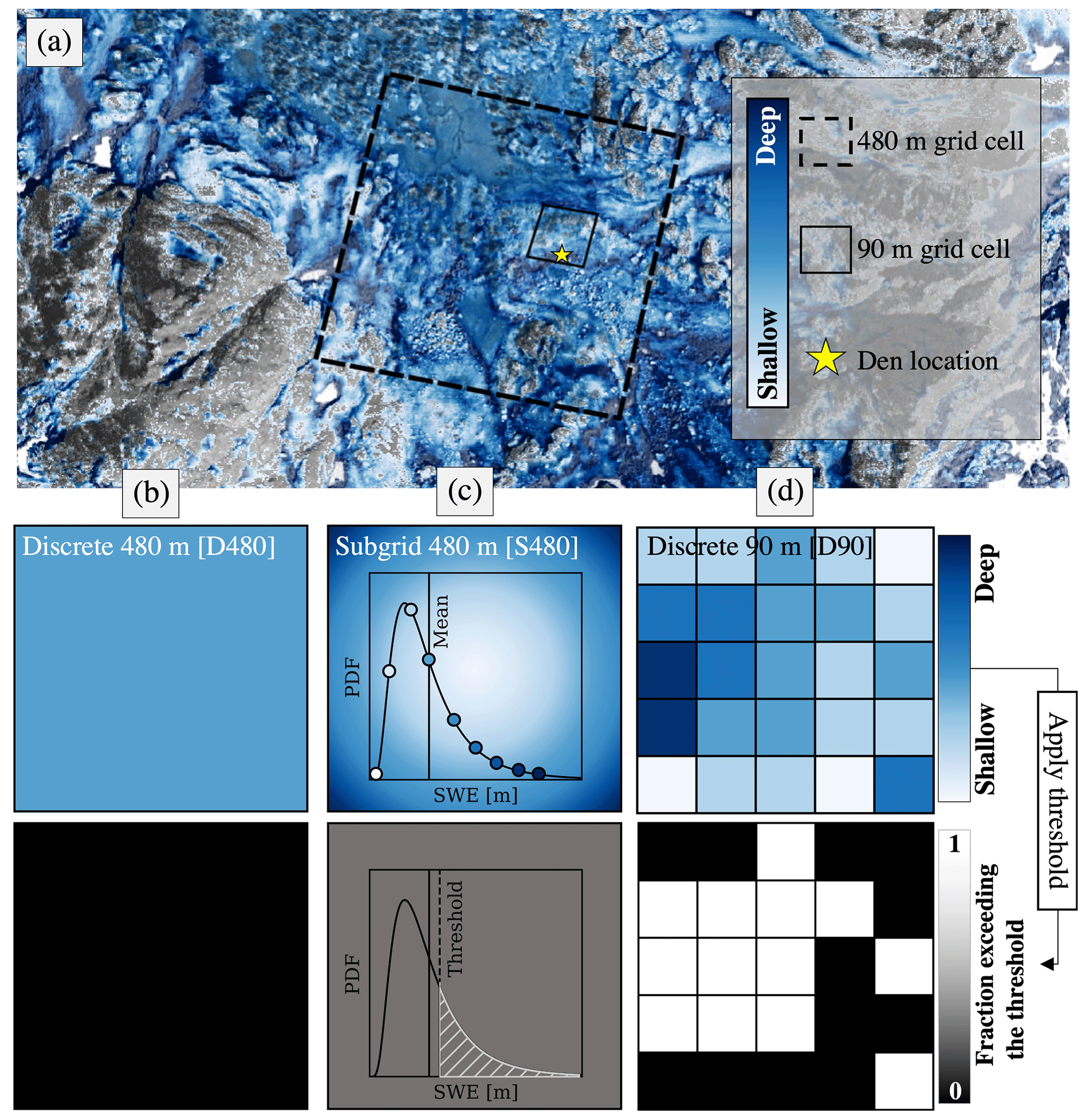
Figure 1SWE spatial heterogeneity inferred from airborne lidar at 1 m resolution, compared to 480 and 90 m grid cells, and a point (star) with a snow drift suitably deep for wolverine denning (a). SWE is simulated in this study using three different spatial discretizations: (b) 480 m discrete grid cells (D480), (c) 480 m grid cells with subgrid SWE heterogeneity (S480), and (d) 90 m discrete grid cells (D90). The fraction of the area that could support wolverine denning is estimated for each discretization using a 0.20 m SWE threshold on 15 May. The fraction of the area exceeding the SWE threshold is binary (fully greater than or less than the threshold) for discrete grid cells (b, d), while the area exceeding the SWE threshold for the S480 discretization (c) is defined by the fraction of the grid cell SWE distribution exceeding the threshold (white hatching)
2.1 Domain
We focused this work over the Rocky Mountain National Park in Colorado state (Fig. 2). This domain is home to several snow-adapted wildlife species and has been included in wolverine habitat assessments (Barsugli et al., 2020; McKelvey et al., 2011; USFWS, 2018). Barsugli et al. (2020) estimated most of the terrain supportive of wolverine habitat in this region to be between 2700 and 3600 m of elevation. Although this area does not currently support a reproductive population of wolverines, this region is of potential interest for wolverine reintroduction. More information about wolverine habitat can be found in the US Fish and Wildlife Service species status assessment (USFWS, 2018).
The Rocky Mountain National Park domain contained several snow observations (Fig 2). These observations include 28 snow telemetry (SNOTEL) stations, deployed and managed by the National Resources and Conservation Service. These stations use snow pillows to measure the weight of snowpack and resulting SWE. A distributed lidar observation of snow depth in the southernmost portion of the domain was also collected by the National Center for Airborne Laser Mapping in May 2010. These observations were used to assess the accuracy of the SWE reanalysis discussed in Sect. 2.2.
2.2 SWE reanalyses
SWE was calculated over the Rocky Mountain domain (Fig. 2) from a popular satellite-era (water years 1985–2020) probabilistic snow reanalysis (Margulis et al., 2019, 2016, 2015) performed at 3 arcsec (∼90 m) and 16 arcsec (∼480 m). This reanalysis was generated at each individual grid cell using an ensemble of simulations forced by the Modern-Era Retrospective analysis for Research and Applications, Version 2 (MERRA-2; Gelaro et al., 2017), and simulated using the simplified Simple Biosphere Model, Version 3 (Xue et al., 1991), coupled with the Liston (2004) snow depletion curve. The forcing dataset was downscaled to the simulation grid (Girotto et al., 2014; Margulis et al., 2015) before running the land surface model. Model ensemble members were provided different (1) precipitation multipliers (influencing total snow mass), (2) snow albedo decay functions (influencing the rate of snow ablation), and (3) parameterizations of subgrid snow spatial variability (influencing subgrid snow cover during snowmelt), among other parameters. The reanalysis then reweighted the ensemble members to most heavily favor those that matched the snowmelt season evolution of fractional snow-covered area from 30 m Landsat observations. We expect uncertainties and errors in the snow reanalysis owing to both errors in meteorological forcing data (e.g., Daloz et al., 2020; Liu and Margulis, 2019) and errors with the snow model (e.g., Feng et al., 2008; Xiao et al., 2021). However, the ensemble approach used by this reanalysis adjusted modeled snow accumulation and depletion to track remote sensing observations of snow cover depletion, which has shown the capability to bias correct SWE and implicitly account for difficult-to-simulate processes like precipitation lapse rates, wind loading and/or scour, avalanching, and forest–snow processes (e.g., Pflug et al., 2022; Yang et al., 2021).
Relative to SNOTEL observations, which are not used by the snow reanalysis, the reanalysis exhibited a SWE coefficient of correlation of 0.82 between 1985 and 2020 in the Rocky Mountain domain (Supplement Fig. S1). On average, the reanalysis was biased low relative to the snow pillow observations by approximately 23 %. However, this could be attributed to the location of SNOTEL observations in forested clearings (Fig. 2a) which typically have SWE deeper than the terrain covered by the 480 and 90 m pixels (e.g., Livneh et al., 2014; Pflug et al., 2022).While the snow reanalysis used in this study is ultimately a model product and subject to a number of modeling uncertainties, the SWE simulated by the 90 and 480 m discretizations agreed closely with each other and with ground observations. Therefore, spatial differences in 15 May SWE and the resulting distribution of snow that exceeded the SWE threshold (e.g., Fig. 1) was attributable to differences in the interactions between the static SWE threshold and different spatial discretizations of snow.
For the 480 m grid cells with subgrid snow variability (Fig. 1c, S480), the heterogeneity of SWE was estimated using a method developed by Liston (2004). This method assumes that the subgrid heterogeneity of SWE accumulation is lognormally distributed and is dictated by a time-constant coefficient of variation (CoV),
where μ is the grid cell mean SWE and σ is the standard deviation of the SWE within that grid cell. The CoV of subgrid SWE accumulation (Fig. 2b and c) was determined for each 480 m grid cell using the most common pattern of SWE accumulation from the overlapping 90 m reanalysis grid cells (Fig. 1d) between 1985 and 2020 (detailed further in Supplement Sect. S1). In Sect. 3.1, we discuss how CoV was used to estimate the temporal evolution of subgrid SWE heterogeneity.
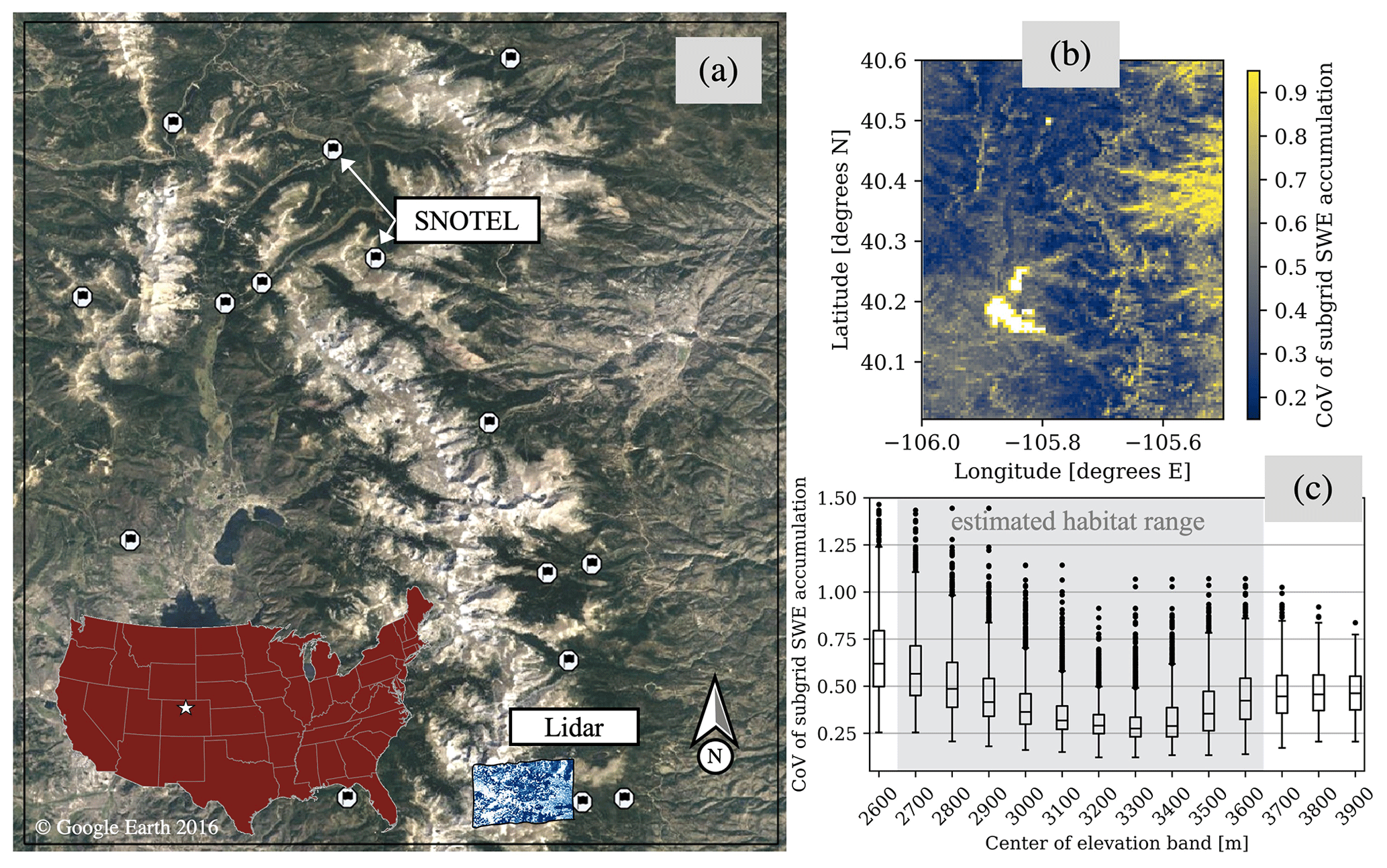
Figure 2Rocky Mountain National Park study domain. The location of SNOTEL observations and lidar snow depth observations are superimposed in the terrain map (a). The 480 m coefficient of variation of subgrid SWE accumulation is shown both spatially (b) and across 100 m elevation bands (c).
The methods evaluate the impacts of snow spatial discretizations and winter climatic conditions on assessments of total area suitable for denning wolverines. We investigated three different spatial discretizations: two discretizations using more common discrete representations of snow, and one with an implicit representation of subgrid snow heterogeneity (see Sect. 3.1). For each, potential wolverine denning area (PWDA) was calculated using a static SWE threshold (0.20 m) on a static spring date (15 May) (Sect. 3.2). Finally, we partitioned years with winter precipitation magnitude and precipitation-phase climate categories (wet, dry, cold, and warm) (see Sect. 3.3). These categories were used to examine whether winter climatic conditions or model representations of snow spatial distribution most influenced estimates of PWDA.
3.1 Subgrid SWE evolution
The temporal evolution of subgrid SWE heterogeneity was estimated for 480 m grid cells (Fig. 1, S480) using methods developed by Liston (2004) (Fig. 3). Provided the reanalysis grid cell mean SWE (μ) from a D480 grid cell (Fig. 1b) and a CoV of subgrid SWE accumulation (Fig. 2b), the probability distribution of subgrid SWE for that grid cell (f(SWE)) was calculated using a lognormal distribution,
Figure 3b demonstrates the subgrid distribution of SWE in two winter periods ( and ) assuming the mean SWE evolution from Fig. 3a, a CoV of 0.50, and Eqs. (2)–(4).
In the snowmelt season, the Liston (2004) methodology assumes spatially uniform snowmelt, causing snow disappearance first in locations with thinner SWE and last in locations with deeper SWE. This can be conceptualized as taking the subgrid distribution of snow at peak SWE (Fig. 3b, ) and adjusting it downwards by a constant amount to reflect spatially uniform melt (SWEm) (Fig. 3c). In doing so, snow only exists for portions of the grid cell where f(SWE) at peak SWE was greater than SWEm. Therefore, the fractional snow-covered area (fSCA) of the grid cell could be calculated from the fraction of the distribution (f(SWE)) with SWE greater than SWEm,
Since SWEm can exceed the amount of SWE that exists in some locations at peak SWE timing, and since SWE cannot be less than 0 m (snow absent), the change in grid cell mean SWE (μ) throughout snowmelt will not necessarily equal SWEm. Rather, μ throughout the snowmelt season can be calculated from the expected value of the melt-shifted distribution (Fig. 3c),
In this study, we were provided μ from the reanalysis at each 480 m grid cell and daily time step. Using the CoV calculated from the overlapping D90 data (Fig. 2b), and maximum annual μ at each grid cell, we calculated the SWE distribution (Eq. 2) for each grid cell at peak SWE timing. Then, using a Newton–Raphson solver, we solved the SWEm for each grid cell that caused μ from Eq. (6) to match D480 μ at each grid cell on 15 May.
The Liston (2004) subgrid SWE parameterization discussed above operates under several assumptions. Like many other studies (e.g., Donald et al., 1995; Helbig et al., 2021; Jonas et al., 2009), Eq. (2) assumes that the distribution of snow accumulation at scales finer than the grid cell resolution can be represented by a lognormal distribution. We tested this assumption by evaluating the distribution of 1 m lidar snow depth observations (Fig. 2a) that fell within 480 m grid cells. The Kolmogorov–Smirnov (KS) statistic, or maximum difference between cumulative distribution functions, was used to test how well different theoretical distributions (e.g., normal, lognormal, gamma, Rayleigh, and chi) used by a variety of snow studies (e.g., He et al., 2019; Helbig et al., 2015; Mendoza et al., 2020; Pflug and Lundquist, 2020; Skaugen and Melvold, 2019) matched the lidar-observed snow depth distributions. The KS statistic for the lognormal distribution (Eq. 2) was 0.12±0.05 and was significantly worse (greater than 0.22) when comparing the observed lidar distributions versus other common distributions, like normal and gamma distributions. While not perfect, these results showed that subgrid snow heterogeneity was approximated best by lognormal distributions. The Liston (2004) subgrid methodology also assumed that the CoV of subgrid SWE accumulation was constant, resulting in a linear increase in SWE variability (standard deviation) with mean SWE throughout the snow accumulation season (Fig. 3b). While we lacked validation data to test this, this assumption is the basis for other modeling approaches, which scale snow input using information from historic snow accumulation patterns (Liston, 2004; Luce et al., 1998; Pflug et al., 2021; Vögeli et al., 2016). Finally, although subgrid snowmelt is not spatially uniform, melt-season snow heterogeneity is often modeled well by assuming uniform snowmelt. This is due to the outsized influence of snow accumulation spatial heterogeneity on snowmelt onset timing and snowmelt rates (Egli et al., 2012; Luce et al., 1998; Lundquist and Dettinger, 2005; Pflug and Lundquist, 2020). Here, we acknowledge that this approach operates on multiple assumptions (discussed above), all of which could vary in accuracy on grid cell level. However, this approach may also provide the opportunity to implicitly represent the heterogeneity of snow in complex terrain and the fraction of the area that could be more supportive for denning habitat (e.g., Fig. 1). We discuss this more in Sect. 3.2. Readers should refer to Liston (2004) for more information about the subgrid snow methodology described in this section.
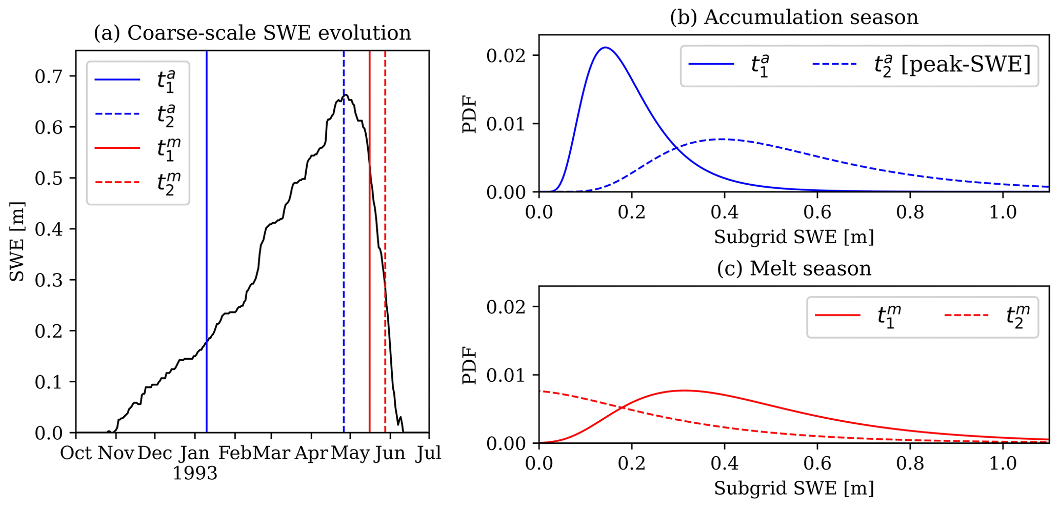
Figure 3An example of the Liston (2004) subgrid SWE parameterization assuming CoV = 0.5 and SWE evolution for a 480 m grid cell in a random year (a). Subgrid SWE distributions are shown for two times (t, subscripts 1 and 2) in the accumulation (superscript a) and melt (superscript m) seasons (b and c, respectively). The timing of each date corresponds to the matching vertical bar in (a).
3.2 Thresholding wolverine habitable area
The area that could support denning wolverines was calculated for each of the discretizations in each year using a SWE threshold of 0.20 m on 15 May, in accordance with previous studies (e.g., Barsugli et al., 2020; Copeland et al., 2010; McKelvey et al., 2011). For the D480 and D90 discretizations, each cell's denning fraction (DF) was classified as fully suitable for denning (DF = 1.0) or unsuitable (DF = 0.0) if the 15 May grid cell SWE was greater than or less than 0.20 m, respectively. For the S480 discretization, DF was calculated for each grid cell using
which represented the portion of the cell's SWE distribution greater than the SWE threshold (β=0.20 m). PWDA was calculated for each discretization as the sum of DF (in space), multiplied by grid cell area.
Relative to DF calculated from a discrete 480 m grid cell (D480), DF calculated over the same area from the finer-scale discretizations (S480 and D90) could have one of four possible relationships. First, the mean SWE of the D480 grid cell and the finer-scale distribution of SWE (S480 and D90) could both be entirely greater than the 0.20 SWE threshold. This results in a fully suitable denning fraction (DF = 1.0) for all discretizations (Fig. 4a). DF would also agree in regions where all discretizations have SWE below 0.20 m (Fig. 4d), resulting in no denning opportunities (DF = 0.0). The scenarios shown in Fig. 4b and c are where DF is sensitive to the discretization. Figure 4b shows a scenario where the coarse-scale mean SWE is sufficiently deep enough to be classified as fully suitable for denning (SWE > 0.20 m), even though some portion of that grid cell contains SWE that is shallower than the SWE threshold. Therefore, using a finer-scale discretization would result in a net loss in DF, the magnitude of which is shown by the red hatching in Fig. 4b. The opposite could be true for instances where coarse-scale mean SWE falls below the 0.20 m SWE threshold, thereby underestimating denning opportunities relative to finer-scale representations that resolve some deeper snow deposits (Fig. 4c, blue hatching). Here, the three reanalysis discretizations (D480, D90, and S480) were provided identical meteorological forcing and, when coarsened to 480m resolution, had SWE that agreed to within 1 %, on average on 15 May. Therefore, the degrees to which the scenarios shown in Fig. 4b and c occur were the drivers of differences to wolverine denning opportunities.
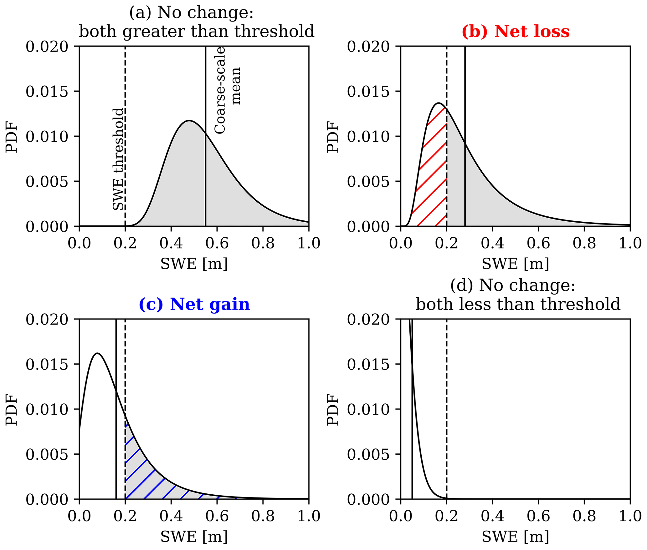
Figure 4Conceptual portrayal of the similarities (a, d) and differences (b, c) in DF for a 480 m discrete grid cell (solid vertical line) and a finer-scale representation (distribution) of SWE over the same area. The dashed vertical lines represent the 0.20 m SWE threshold. Shaded areas show the portion of the distribution with SWE greater than the threshold. Hatched areas demonstrate differences in DF between the coarser-scale and finer-scale discretizations of SWE.
3.3 Categorizing winter climate categories
To determine PWDA sensitivity to different climatic conditions, we identified years from the reanalysis with different winter precipitation magnitude and phase (rain versus snow). Here, winter is defined by periods between 1 October and the date of domain peak SWE volume. Following work from Heldmyer et al. (2023), we used domain average cumulative winter precipitation and the fraction of the winter precipitation that fell as snow (both from the reanalysis) as indices for winter precipitation magnitude and the temperature at which precipitation fell. Using a percentile, we separated years that fell at least that far from the 1985–2020 median precipitation magnitude and fraction of snow precipitation. In doing so, we partitioned years with wet, dry, cold, and warm winter climate categories. We did this separation using a range of percentiles until the statistical difference (measured using the Mann–Whitney u test) in D480 PWDA was maximized between the years with different climatic conditions (warm, cold, wet, dry, and typical). To avoid spurious results, this percentile was also adjusted to ensure that each climate category included at least 6 years. This approach maximized the difference in interannual PWDA as a function of different winter climatic conditions. This was then used as the baseline to compare how much more or less sensitive PWDA was to the different SWE spatial discretizations.
Over low-elevation forested grid cells (< 2800 m), SWE accumulation variability was large relative to the smaller amounts of snow, resulting in large CoV (typically between 0.50 and 0.80) (Fig. 2b and c). On mid-elevation slopes (2800–3300 m), CoV tended to be smaller (approximately 0.30, on average). However, CoV increased again at higher elevations (> 3300 m) and particularly on the leeward side of peaks. This was expected given the more extreme terrain and increased spatial variability of snow from wind drifting, preferential deposition, cornice formation, and avalanching.
The difference in PWDA was maximized between (1) warm and cold years and (2) wet and dry years that had winter precipitation magnitude (Fig. 5a, x axis) and precipitation phase (Fig. 5a, y axis) that fell above the 77th and below the 23rd percentiles (±27th percentile from the median). These climate conditions had impacts on the evolution of SWE and snow-covered area (Fig. 5b and c). On average, as compared to years with normal winter precipitation magnitude and phase (Fig. 5a, white region), cold years and wet years had peak SWE volume that was 23 % and 28 % greater, respectively. This was opposed to warm years and dry years, with peak SWE volume that was 21 % and 31 % smaller, on average, than typical water years. The timing of peak SWE was driven most by the magnitude of winter precipitation. In fact, average peak SWE timing was 28 d later for wet years than dry years. Snow disappearance timing (snow-covered area < 200 km2) was also 21 d later for wet years than dry years. Statistically, the timing of snow disappearance, crucial for wolverine denning habitat, was explained well by the peak SWE volume (r= 0.82) and the date of peak SWE (r= 0.63), both of which were influenced more by winter precipitation magnitude than temperature.
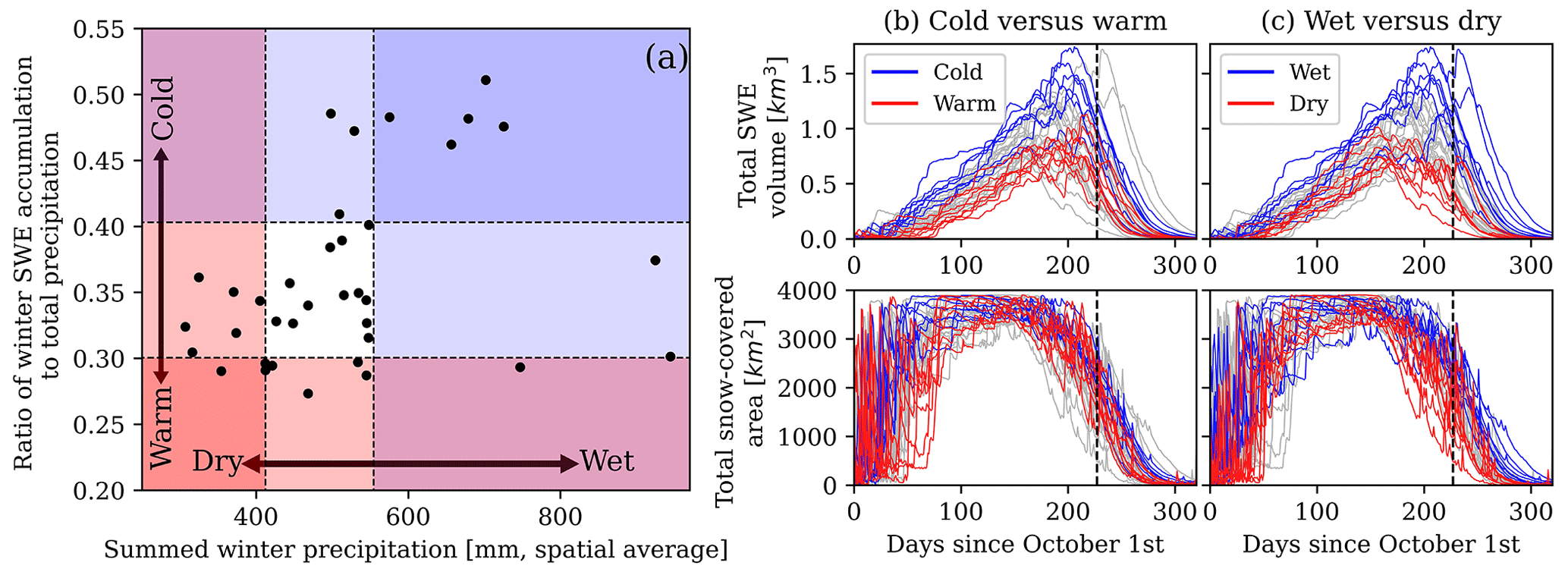
Figure 5Annual climatic conditions grouped into categories based on winter precipitation magnitude (a, horizontal axis) and precipitation phase (a, vertical axis) outside the 23rd and 77th percentiles (a, dashed lines). The evolution of SWE volume and snow cover are compared for warm versus cold (b) and wet versus dry years (c). Dashed vertical lines in (c) and (d) indicate 15 May.
In all years except dry 2002, PWDA was smaller for the D90 discretization than the D480 discretization (Fig. 6). This resulted in a 10 % reduction to the 36-year median PWDA (Fig. 6b). The PWDA differences between the D480 and S480 discretizations varied more on an annual basis. For years with D480 PWDA less than 1000 km2, S480 discretizations increased PWDA by up to 30 %; 11 % on average. However, in years with PWDA greater than 1000 km2, S480 PWDA was approximately 3 % smaller, on average, than D480 PWDA. In short, the S480 discretization tended to have smaller annual swings in PWDA than the D480 discretization. The causes of these PWDA disagreements are discussed in Sect. 5.1. Despite the annual differences in D480 and S480 PWDA, the 36-year median PWDA for these discretizations agreed to within 1 % (Fig. 6b).
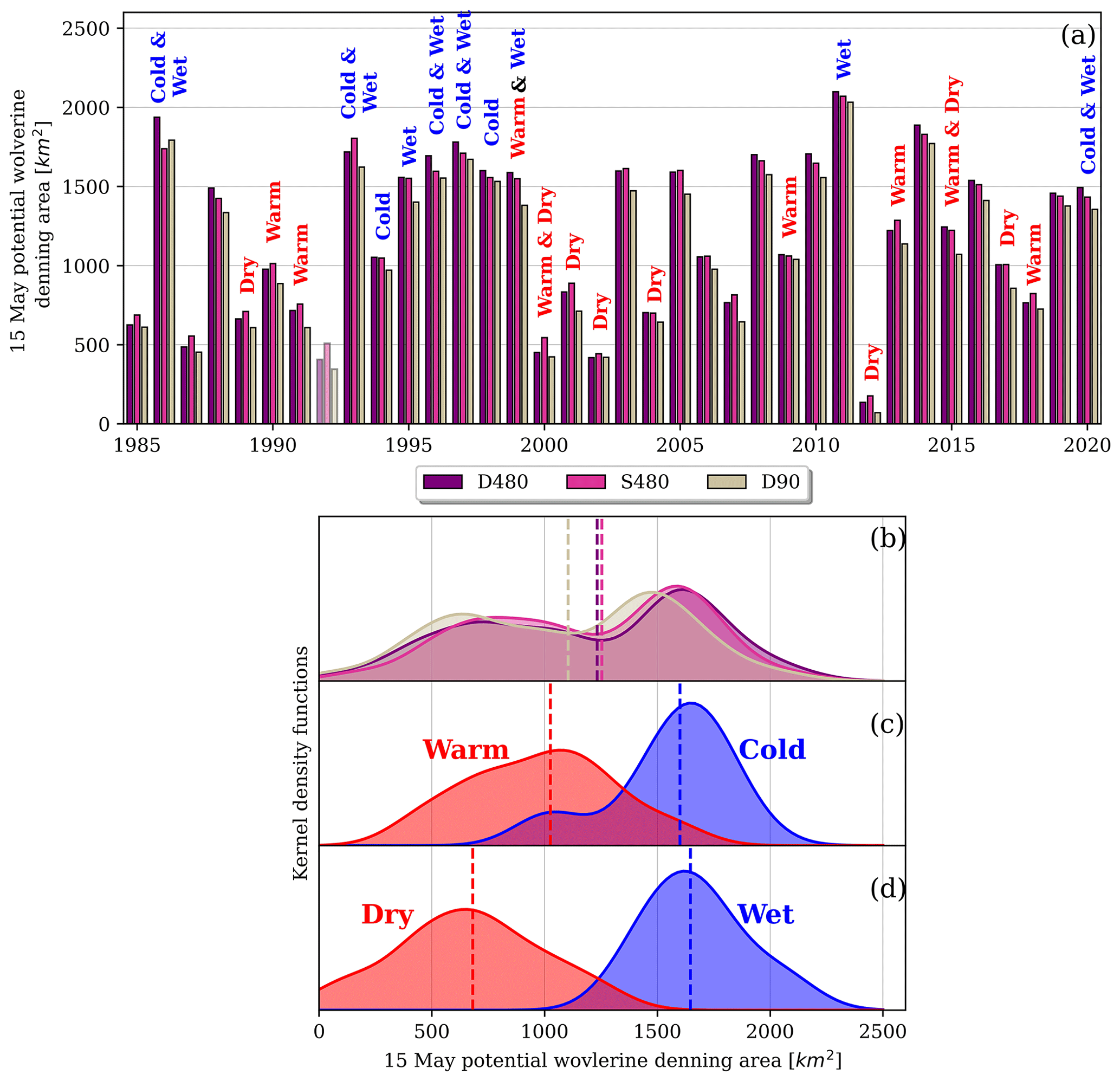
Figure 615 May PWDA compared annually for three different spatial discretizations (a). Lower panels show the kernel distributions for the data in (a), separated based on the spatial discretization (b), temperature categories (c), and precipitation categories (d). The medians of each distribution are shown by the dashed vertical lines (b–d). The data in (c) and (d) include data from all three spatial discretizations. The data from WY1992 (a, faded bars) exhibited artifacts and were excluded from the kernel distributions (b–d).
Even though PWDA was sensitive to different spatial discretizations (Fig. 6b), PWDA across the 36-year period was not statistically different between any of the three discretizations (p > 0.48). Conversely, the difference in 15 May PWDA was significantly larger between the years with different winter climate categories (Fig. 6c and d).Differences in PWDA between years with warm and cold conditions were statistically significant (). Given that the 15 May snow-covered areas were similar between warm and cold years (Fig. 5b), this difference between warm and cold years in Fig. 6c shows that changes to PWDA were driven by changes to SWE magnitude and the area with SWE exceeding the SWE threshold. Dry and wet years exhibited larger differences to both 15 May SWE and snow cover (Fig. 5c), resulting in PWDA (Fig. 6d) that was even more different between the years with these climate conditions (). The impact of these warm, dry, cold, and wet climate conditions resulted in the bimodal distributions in PWDA shown for the different discretizations across the full time period (Fig. 6a). While PWDA was not statistically different between cold and wet years (p= 0.34), the distribution of PWDA in dry years was significantly smaller than the distribution of PWDA in warm years (p= 0.001), showing that PWDA was more sensitive to conditions that reduced snow habitat, like warm and dry conditions.
The results from Fig. 6 suggested that changes in PWDA across annual periods of differing climatic conditions or across future periods with expected changes in climate (e.g., Barsugli et al., 2020) should be informative from a species status assessment perspective, regardless of the snow spatial discretizations that we tested here. However, as noted above, the S480 discretization increased PWDA by 11 % on average in low-snow years, with increases as large as 30 % for individual years. These low-snow years often corresponded with drier and/or warmer winter conditions, the latter of which are expected in the future. For example, the average air temperature during December, January, and February precipitation events during warm years in the reanalysis record was approximately 0.8∘ higher than winter precipitation events in typical years. These conditions are consistent with what is projected for this region by 2055 (Eyring et al., 2016; Scott et al., 2016). This suggests that the disparity between habitat inferred from discrete grid cells and grid cells with subgrid snow heterogeneity could be of greater importance for future snow habitat assessments. Additionally, using PWDA as the sole metric for evaluating differences in annual opportunities for wolverine denning may oversimplify the degree to which static thresholds and different spatial discretizations interact. For instance, PWDA inferred on a static date (15 May) compares very different regimes of the snow season, as wet years had peak SWE timing, and snowmelt season onset, that was 21 d later than typical snow seasons (Fig. 5). Since shallower snow melts more readily than deeper snow (provided the same energy), comparing SWE on a static date in years with very different conditions neglects the different rates of habitat depletion for a few days on either side of the date threshold. These issues are investigated more in Sect. 5.
In this section, we diagnose the causes for disagreements in the frequency and locations at which the 15 May SWE exceeded the 0.20 m SWE threshold between the three spatial discretizations of snow (Sect. 5.1). We also investigate how the use of a static SWE threshold and threshold date may obscure the picture of interannual changes to wolverine denning habitat availability (Sect. 5.2). Using these findings, we discuss how information provided from multiple spatial discretizations could provide information about the fidelity and uncertainty of thresholds, as well as the interactions and tradeoffs between spatial discretizations and thresholds, both in context for assessing snow-adapted wildlife habitat and more broadly for other environmental studies (Sect. 5.3).
5.1 Spatial differences in DF
The spatial difference in DF between the three discretizations had annually similar patterns, with the largest differences at locations where the domain had SWE that was near the 0.20 m SWE threshold. This is shown in Fig. 7d and Fig. 7e where the spatial DF disagreements that spiked on 15 May 2008 were focused between approximately 2800 and 3200 m of elevation. Relative to the D480 discretization, the S480 discretization tended to increase DF in grid cells at lower elevations where mean SWE was less than the SWE threshold, but some portion of the grid cell had SWE deep enough to exceed the threshold (e.g., Fig. 4c). The opposite effect occurred at higher elevations where mean SWE exceeded the SWE threshold, but the lower tails of the S480 SWE distributions were below the threshold (e.g., Fig. 4b). As a result, the S480 discretization had a more gradual increase in thresholded denning availability with elevation and a downward shift in the elevations that could support denning wolverines (Fig. 7f). In fact, relative to the D480 discretization, the S480 discretization had 23 % less interannual variability in the elevation at which equal PWDA existed at higher and lower elevations (Fig. S2a). This was a result of the subgrid representations of SWE heterogeneity which allowed for gradual and fractional (0.0 ≤ DF ≤ 1.0) increases in DF with increases in SWE. This was opposed to the D480 discretization, which could only resolve binary DF (0 or 1 for SWE less than and greater than 0.20 m), resulting in larger elevational shifts in the annual locations that could support wolverine denning.
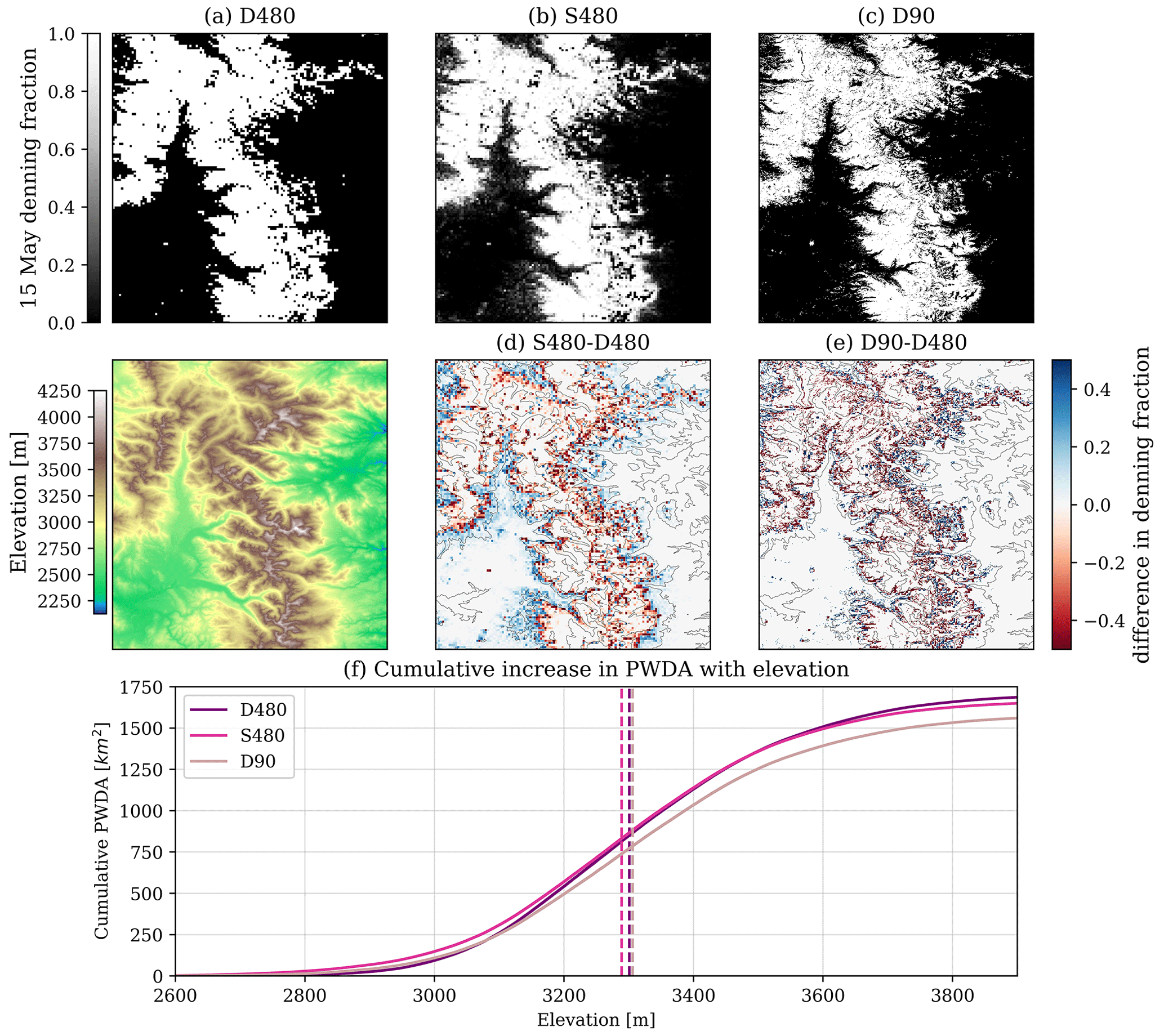
Figure 7Spatial comparisons of DF for the three discretizations on 15 May 2008. Panel (f) compares the cumulative PWDA (y axis) calculated for grid cells sorted in order of increasing elevation (x axis). Dashed vertical dashed lines show the elevation of median PWDA or elevation at which PWDA is equal for higher and lower elevations.
Relative to the D480 discretization, the D90 discretization also tended to increase DF at lower elevations. However, all years had reduced D90 DF in elevations higher than approximately 3120 m. This was the cause of the 10 % reduction in D90 PWDA, relative to the other discretizations (Fig. 6b). These decreases were typically located on unvegetated, exposed, and steep slopes, where it was likely that winter snow retention was decreased, snow sublimation was increased, and sloughing to lower elevations was more common (Bernhardt and Schulz, 2010; Grünewald et al., 2014; Machguth et al., 2006). This demonstrates the utility of the observation-based reanalysis used in this study, which may have resolved thinner snow deposits on slopes with decreased snow retention and/or enhanced snow removal by processes like sloughing, both of which are among the most difficult processes to represent with models. The D480 discretization averaged snow from surrounding areas, smoothing out thinner snow deposits resolved by the D90 discretization. Although attempting to resolve subgrid snow heterogeneity, the evolution of SWE assumed by the S480 simulation, which assumed lognormal snow accumulation and spatially uniform subgrid snowmelt (Fig. 3), may have been less appropriate for the areas containing sparsely distributed 90 m regions with thinner snow. While the D90 discretization decreased total PWDA, D90 snow cover was also patchier (Fig. 7c), which could also influence the movement and connectivity for wolverines (USFWS, 2018) and other snow-adapted species.
Winter precipitation magnitude and temperature influenced the volume of snow and the elevation of the snow line that existed on 15 May in each year. Since the differences in DF between the discretizations were largest at grid cells near the 0.20 m SWE threshold, often located just above the snow line, the spatial pattern of DF differences (e.g., Fig. 7) exhibited an interannually repeatable relationship with the dry, warm, cold, and wet winter climate categories (Fig. 5). To show this, we calculated the differences in DF between all three discretizations (D480 versus S480, D480 versus D90, and S480 versus D90) in all 36 years. Then, for each 480 m grid cell, we identified the climate category that resulted in the greatest mean absolute differences in DF across the three discretizations. The climate categories that had the greatest influence on DF uncertainties covered similar portions of the domain, with 33.7 %, 20.9 %, 25.2 %, and 20.2 % being most attributed to dry, warm, cold, and wet conditions, respectively (Fig. 8). At low elevations (2650–3050 m), 15 May snow typically existed only in wet years. In those years and elevations, mean SWE for the D480 and D90 discretizations often fell below the 0.20 m SWE threshold. However, the large CoVs of subgrid SWE accumulation in these elevations (Fig. 2) resulted in S480 subgrid SWE distributions with upper tails that sometimes exceeded 0.20 m (e.g., Fig. 4c) (Fig. 8c). This was in line with findings from Magoun et al. (2017), who noted suitable denning conditions at lower elevations, even in instances when the surrounding terrain was predominantly snow free.
The average differences in DF between the three discretizations were largest in cold years for elevations spanning 3050–3150 m and in warm years for elevations spanning 3150–3350 m (Fig. 8). Across this elevation range (3050–3350 m), both of the 480 m discretizations (D480 and S480) estimated more denning opportunities than the D90 discretization (Fig. 8c). However, at higher elevations (> 3350 m), DF calculated from the S480 discretization approached DF calculated from the D90 thinner snow deposits (Fig. 8c).
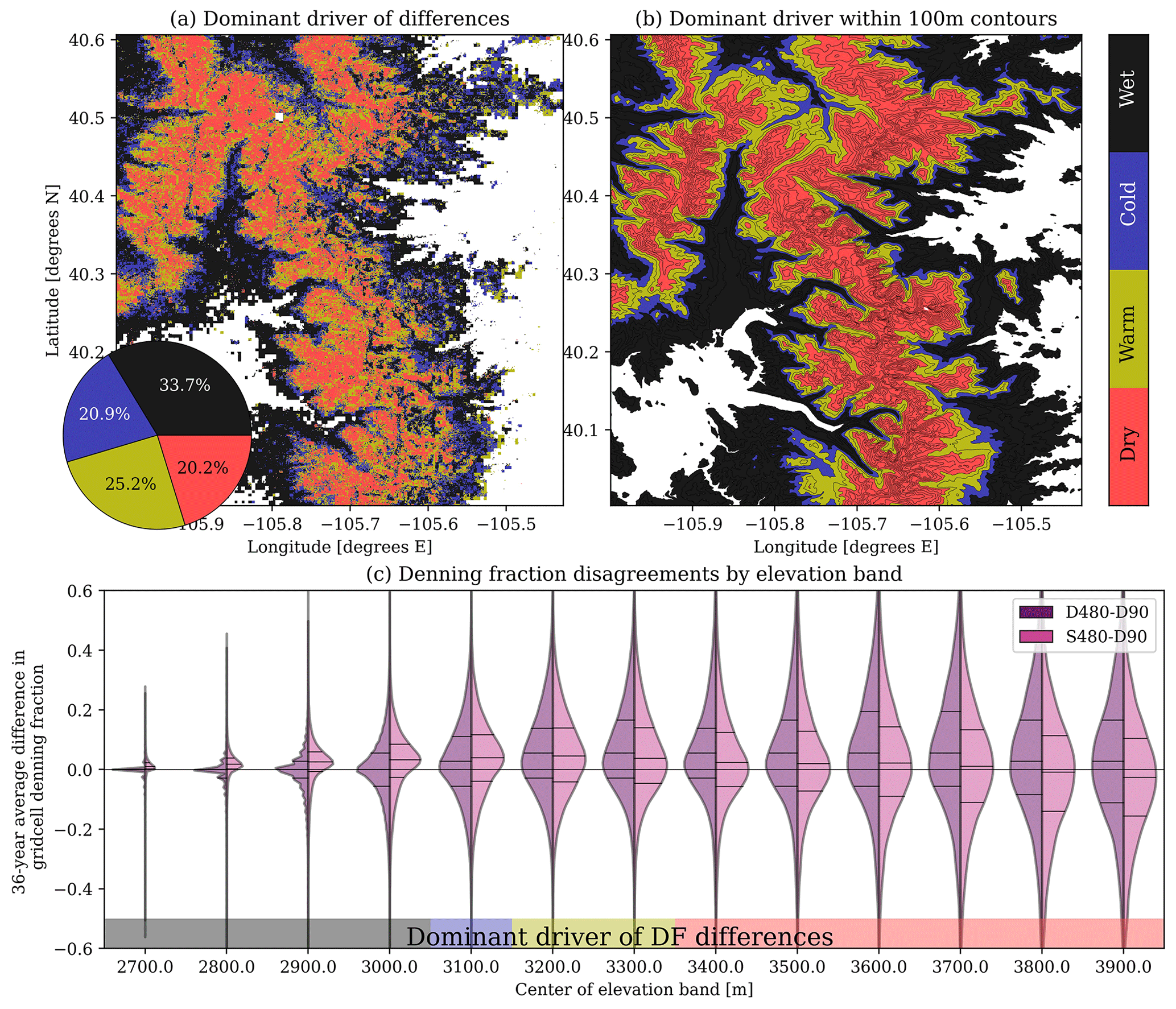
Figure 8Winter climate categories that most influenced DF disagreements between the three discretizations (a). Panel (b) shows the most prevalent influence from (a), for 100 m elevation bands. Using DF from the D90 discretization as a reference, the 36-year average difference in DF for the D480 and S480 simulations are shown by distributions for each 100 m elevation band (c). Lines inside the distributions show the median and interquartile range.
5.2 Threshold sensitivities
To this point, we assumed confidence in the SWE (0.20 m) and date (15 May) thresholds. However, small changes to either threshold could influence annual estimates of PWDA (e.g., Copeland et al., 2010; Magoun et al., 2017). In Fig. 9, we show PWDA calculated from a range of realistic SWE thresholds and threshold dates. The range of SWE thresholds (0.20 ± 0.07 m) were determined using a snow depth of 0.50 m, corresponding to observed wolverine dens (USFWS, 2018) and the 90th percentile range of 15 May snow densities from SNOTEL observations (Fig. 2a) between 1985 and 2020 (260–540 kg m−3). The range of threshold dates spanned a period of ± 2 weeks, corresponding to the difference in peak SWE timing between dry and wet years (Fig. 5). This month-long time span is also consistent with the observed range of wolverine birth dates (Inman et al., 2012). PWDA sensitivity was calculated using all combinations of SWE and date thresholds, both of which were discretized at 14 equally spaced increments (Fig. 9, left). Then, the gradients (direction and magnitude of greatest change in PWDA) were calculated from each unique combination of SWE and date thresholds. The gradients were summed using vector addition (Fig. 9, right column) to determine (1) the total rate of change in PWDA with changing thresholds (arrow length) and (2) the degree to which PWDA was sensitive to one threshold versus the other (arrow angle). This process was repeated for each discretization and year.
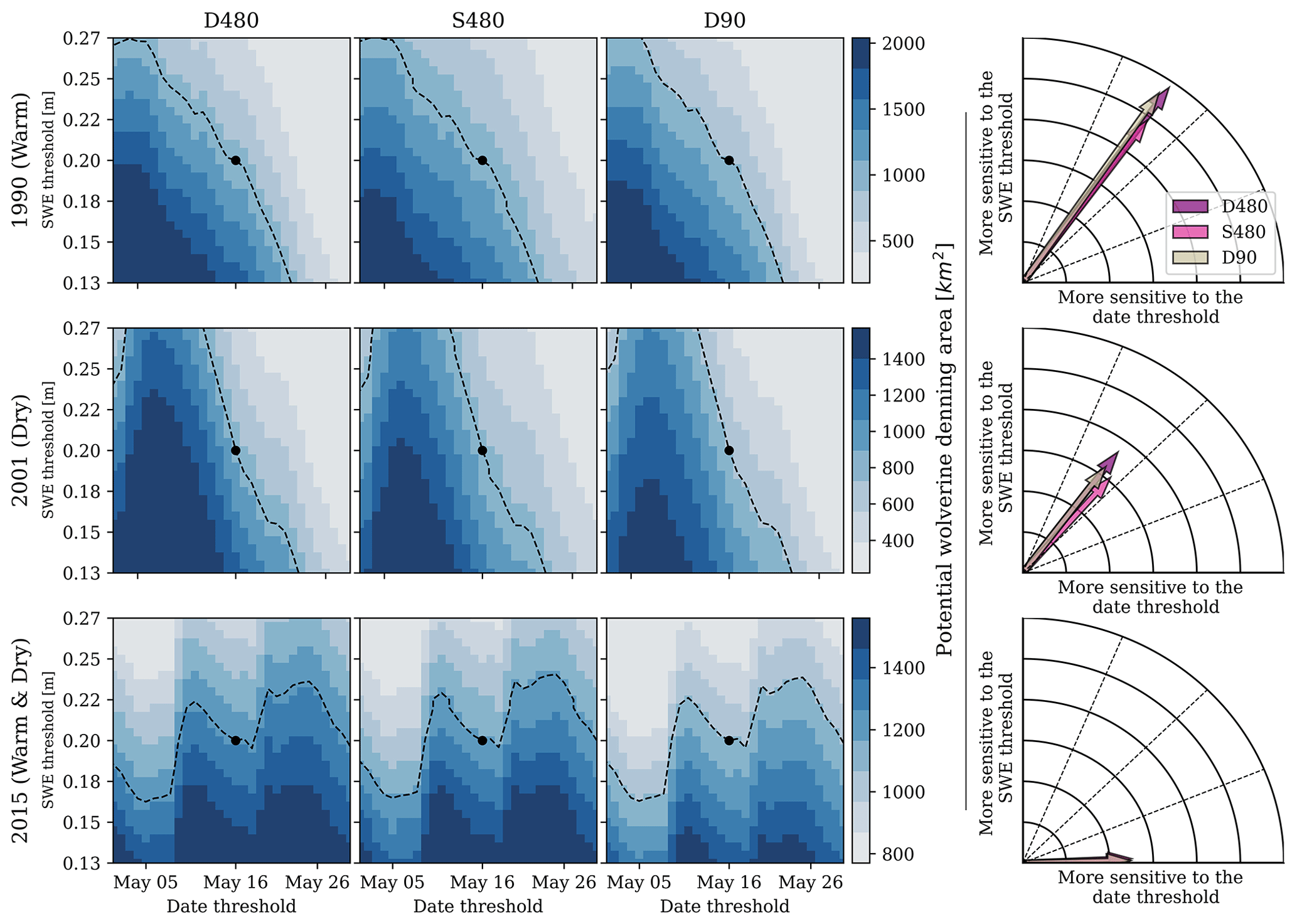
Figure 9PWDA calculated using different SWE (y axes) and date thresholds (x axes), for the different discretizations (columns), in 3 different years (rows) with very different sensitivities. PWDA calculated from the default thresholds (0.20 m SWE on 15 May) is shown by the black circle. Combinations of thresholds that could reproduce the default PWDA are approximated by the dashed contour. The rightmost arrows show the total direction and magnitude of PWDA changes with changes in the thresholds.
PWDA in warm 1990 was 18 % more sensitive to the SWE thresholds than the threshold dates (Fig. 9, top row). To put this another way, the change in PWDA across a period of ±3 d from 15 May was approximately equal to the change in PWDA from adjusting the SWE threshold by ±2.5 cm. This sensitivity was similar to the average threshold sensitivity from the 36-year reanalysis record (Fig. S2b). However, multiple years exhibited unique sensitivities. For example, spring snowfall between 1 and 6 May 2001 (Fig. 9, middle row) caused PWDA to both increase and decrease over the range of date thresholds (assuming a constant SWE threshold). Therefore, PWDA changed based on whether the threshold date was before, during, or after the May snowfall event, buffering the degree to which thresholded denning habitat estimates were influenced by the specific winter meteorological conditions that occurred in that year. This effect also occurred in 2015, when 15 May fell between two spring snowfall events (Fig. 9, bottom row). As a result, PWDA tended to increase, on average, over the range of threshold dates, resulting in heightened sensitivities to the date on which denning opportunities were evaluated. These spring snowfall events had large impacts on 15 May PWDA but are unlikely to accurately represent the habitat opportunities and stresses that wolverine were subject to in that year. This demonstrates the dangers of thresholds applied on static dates and suggests that metrics over multiple dates (e.g., number of May days exceeding a SWE threshold) and across sequences of years could be more accurate representations of snow refugia.
PWDA varied by as much 82 % between the realistic thresholds shown in Fig. 9. This was similar in magnitude to the differences in PWDA between years with opposing winter climate anomalies (Fig. 6c and d). Across the years evaluated in this study, the sensitivities to the thresholds were largest for the D480 simulation and smallest for the S480 simulation (Figs. 9 and S2b). As discussed in Sect. 5.1, the S480 discretization, which represented subgrid snow distribution and fractional changes to DF with changes to the SWE threshold and threshold date, had less sensitivity to annual changes in meteorological conditions. Similarly, small changes in the SWE threshold and threshold date changed the prevalence of snow that exceeded the static threshold for discrete grid cells by larger amounts than the S480 discretization. This suggests that studies with subgrid representations of snow heterogeneity may decrease the overall sensitivity to SWE and date thresholds.
5.3 Threshold caveats and future suggestions
The D90 and S480 discretizations provided unique but different advantages for estimating PWDA. We believe that the upper-elevation decreases in D90 SWE and denning habitat on steep and unvegetated surfaces were realistic. These results were contrary to the findings from Barsugli et al. (2020), who in the same domain, found that finer-scale physically based simulations resulted in net increases in wolverine denning opportunities. However, this analysis used a joint model and observation-based approach (Sect. 2) that may have implicitly represented decreased snow retention and/or snow sloughing better than the physically based models used by Barsugli et al. (2020). The discretization with subgrid snow heterogeneity (S480), which is not as commonly used, had less dramatic swings in PWDA with changes in annual winter climatic conditions (Fig. 6) and thresholds (Fig. 9). We therefore think that subgrid representations of snow may be important for habitat assessments, especially given that snow deposits suitable for denning at scales of 10 m or less sometimes occur in regions with otherwise little snow (Magoun et al., 2017).
The results of this study suggest that uncertainties provided from combinations of multiple discretizations, applied across a range of realistic thresholds, would be more informative than a single discretization and set of thresholds. For instance, SWE volume on 15 May 2015 was 10 % less than the 36-year median 15 May SWE volume. However, due to spring snowfall (Fig. 9), SWE volume on 30 May 2015 was 31 % greater than the 36-year median on the same date. Multiple discretizations could also be used to identify the locations of most (e.g., Fig. 4a and d) and least certain (Fig. 4b and c) opportunities for denning habitat. This information could be used as the basis for identifying the locations where remote sensing or field campaigns could hone annual estimates of refugium, given that year's meteorological conditions. Altogether, differences across discretizations (e.g., Fig. 6) and threshold sensitivities (e.g., Fig. 9) could also be used to provide uncertainty bounds for PWDA calculated in any given year.
Our results show that caution is warranted when combining gridded data and static thresholds. While we focus on the impact that thresholds and different snow spatial discretizations have on approximations of wolverine denning opportunities, we expect these results to be applicable to other environmental applications. For instance, while temperature thresholds are widely used to partition rain and snow precipitation in models, temperature discretized at different spatial scales could influence the spatial variability of temperature and resulting snowfall volume thresholded across one or many snowfall events (e.g., Jennings et al., 2018; Nolin and Daly, 2006; Wayand et al., 2017). Snow cover thresholded using visible and infrared satellite observations may also require changes based on the size of the satellite pixels and the underlying topographic and vegetative characteristics (Härer et al., 2018; Pestana et al., 2019). Future studies should report the extent to which different spatial discretizations and ranges of realistic thresholds influence results. This information could be used to report (1) the uncertainty of thresholded outputs, (2) the fidelity of different gridded products, and (3) the degree to which multiple spatial discretizations could be combined to improve the fidelity and transferability of results.
Potential wolverine denning area (PWDA) was thresholded using a published SWE threshold (0.20 m) on a threshold date (15 May) in a Colorado Rocky Mountain domain between 1985 and 2020. Results showed that PWDA was statistically different (p < 0.01) between years with different winter precipitation magnitude (wet versus dry) and precipitation temperature (cold versus warm) conditions. In fact, climate-driven differences in annual PWDA were substantially larger than differences in PWDA between snow discretized using (1) discrete 480 m grid cells, (2) 480 m grid cells with subgrid representations of SWE heterogeneity, and (3) discrete 90 m grid cells. Therefore, studies that assess changes in habitat health for species like wolverines with past and future changes in climate could be informative, regardless of the spatial discretizations tested.
Despite the sensitivity to winter climatic conditions, annual differences in denning patterns and parameter sensitivities emerged for the different discretizations. For instance, 90 m grid cells resolved thinner snow deposits in mid-to-upper elevations (approximately 3050–3350 m) that were not resolved by either of the 480 m discretizations, decreasing PWDA by 10 %, on average. Snow discretized with subgrid representations of SWE spatial heterogeneity also had less dramatic swings in annual PWDA. The simulations with subgrid SWE heterogeneity increased PWDA by 10 %–30 % in low-snow years, many of which were representative of future changes in average temperature expected over the next 50 years. Spatially, the differences in the prevalence of SWE that exceeded the threshold between the three different snow discretizations were heightened at the grid cells that had SWE values close to the SWE threshold (0.20 m) on 15 May, the elevation of which was driven in large part by the winter climatic conditions. On average, PWDA was more sensitive to the SWE threshold than the date threshold but had the smallest amount of sensitivity to the 480 m simulation with subgrid snow heterogeneity, which had more gradual changes to the fraction of a region exceeding the SWE threshold with small changes in SWE. This discretization also had the least amount of sensitivity to interannual changes in winter climatic conditions. However, some years had late spring snowfall events, altering the amount of PWDA by up to 82 % depending on whether the threshold date was before, during, or after the snowfall event.
Our results show that differences in how snow is spatially discretized can influence information generalized using thresholds. Therefore, future studies thresholding spatiotemporal environmental data should include multiple spatial discretizations and ranges of realistic thresholds to provide a more comprehensive picture of uncertainties associated with chosen thresholds and datasets. Although we used wolverine habitat as an example, we expect these results to be applicable to any study thresholding environmental data, especially for studies generalizing information at spatial scales finer than those of modeled or observed resolutions.
Readers are encouraged to enquire about the most up-to-date version of the reanalysis from the principal developer, Steven Margulis. Scripts used in this paper are provided at https://github.com/jupflug/HABITAT-threshold_vs_discretization (last access: 18 July 2023; https://doi.org/10.5281/zenodo.8161074, Pflug, 2023).
The supplement related to this article is available online at: https://doi.org/10.5194/hess-27-2747-2023-supplement.
JMP and BL designed the experiments. YF and SM provided the snow reanalysis. JMP wrote the paper, with comments provided from all authors and special supervision by BL.
The contact author has declared that none of the authors has any competing interests.
Publisher’s note: Copernicus Publications remains neutral with regard to jurisdictional claims in published maps and institutional affiliations.
We would like to thank and acknowledge support from current and past US Fish and Wildlife Service staff, in particular, John Guinotte and Steve Torbit.
This research has been supported by the Cooperative Institute for Research in Environmental Sciences (grant no. 00782920) and the US Geological Survey, Western Ecological Research Center, US Geological Survey (grant no. G21AC10645).
This paper was edited by Jan Seibert and reviewed by two anonymous referees.
Araújo, M. B. and Peterson, A. T.: Uses and misuses of bioclimatic envelope modeling, Ecology, 93, 1527–1539, https://doi.org/10.1890/11-1930.1, 2012.
Auer, A. H.: The Rain versus Snow Threshold Temperatures, Weatherwise, 27, 67, https://doi.org/10.1080/00431672.1974.9931684, 1974.
Barsugli, J. J., Ray, A. J., Livneh, B., Dewes, C. F., Heldmyer, A., Rangwala, I., Guinotte, J. M., and Torbit, S.: Projections of Mountain Snowpack Loss for Wolverine Denning Elevations in the Rocky Mountains, Earths Future, 8, e2020EF001537, https://doi.org/10.1029/2020EF001537, 2020.
Bernhardt, M. and Schulz, K.: SnowSlide: A simple routine for calculating gravitational snow transport, Geophys. Res. Lett., 37, L11502, https://doi.org/10.1029/2010GL043086, 2010.
Boelman, N. T., Liston, G.E ., Gurarie, E., Meddens, A. J. H., Mahoney, P. J., Kirchner, P. B., Bohrer, G., Brinkman, T. J., Cosgrove, C. L., Eitel, J. U. H., Hebblewhite, M., Kimball, J. S., LaPoint, S., Nolin, A. W., Pedersen, S. H., Prugh, L. R., Reinking, A. K., and Vierling, L. A.: Integrating snow science and wildlife ecology in Arctic-boreal North America, Environ. Res. Lett., 14, 010401, https://doi.org/10.1088/1748-9326/aaeec1, 2019.
Bokhorst, S., Pedersen, S. H., Brucker, L., Anisimov, O., Bjerke, J. W., Brown, R. D., Ehrich, D., Essery, R. L. H., Heilig, A., Ingvander, S., Johansson, C., Johansson, M., Jónsdóttir, I. S., Inga, N., Luojus, K., Macelloni, G., Mariash, H., McLennan, D., Rosqvist, G. N., Sato, A., Savela, H., Schneebeli, M., Sokolov, A., Sokratov, S. A., Terzago, S., Vikhamar-Schuler, D., Williamson, S., Qiu, Y., and Callaghan, T. V.: Changing Arctic snow cover: A review of recent developments and assessment of future needs for observations, modelling, and impacts, Ambio, 45, 516–537, https://doi.org/10.1007/s13280-016-0770-0, 2016.
Cayan, D. R.: Interannual Climate Variability and Snowpack in the Western United States, J. Climate, 9, 928–948. https://doi.org/10.1175/1520-0442(1996)009<0928:ICVASI>2.0.CO;2, 1996.
Clark, M. P., Nijssen, B., Lundquist, J., Kavetski, D., Rupp, D. E., Woods, R. A., Freer, J. E., Gutmann, E. D., Wood, A. W., Brekke, L. D., Arnold, J. R., Gochis, D. J., and Rasmussen, R. M.: A unified approach for process-based hydrologic modeling: 1. Modeling concept, Water Resour. Res., 51, 2498–2514, https://doi.org/10.1002/2015WR017198, 2015.
Copeland, J. P., McKelvey, K. S., Aubry, K. B., Landa, A., Persson, J., Inman, R. M., Krebs, J., Lofroth, E., Golden, H., Squires, J. R., Magoun, A., Schwartz, M. K., Wilmot, J., Copeland, C. L., Yates, R. E., Kojola, I., and May, R.: The bioclimatic envelope of the wolverine (Gulo gulo): do climatic constraints limit its geographic distribution?, Can. J. Zool., 88, 233–246, https://doi.org/10.1139/Z09-136, 2010.
Daloz, A. S., Mateling, M., L'Ecuyer, T., Kulie, M., Wood, N. B., Durand, M., Wrzesien, M., Stjern, C. W., and Dimri, A. P.: How much snow falls in the world's mountains? A first look at mountain snowfall estimates in A-train observations and reanalyses, The Cryosphere, 14, 3195–3207, https://doi.org/10.5194/tc-14-3195-2020, 2020.
Dierauer, J. R., Allen, D. M., and Whitfield, P. H.: Snow Drought Risk and Susceptibility in the Western United States and Southwestern Canada, Water Resour. Res., 55, 3076–3091, https://doi.org/10.1029/2018WR023229, 2019.
Donald, J. R., Soulis, E. D., Kouwen, N., and Pietroniro, A.: A Land Cover-Based Snow Cover Representation for Distributed Hydrologic Models, Water Resour. Res., 31, 995–1009, https://doi.org/10.1029/94WR02973, 1995.
Dozier, J.: Spectral signature of alpine snow cover from the landsat thematic mapper, Remote Sens. Environ., 28, 9–22, https://doi.org/10.1016/0034-4257(89)90101-6, 1989.
Durner, G. M., Simac, K., and Amstrup, S. C.: Mapping Polar Bear Maternal Denning Habitat in the National Petroleum Reserve – Alaska with an IfSAR Digital Terrain Model, Arctic, 66, 197–206, 2013.
Egli, L., Jonas, T., Grünewald, T., Schirmer, M., and Burlando, P.: Dynamics of snow ablation in a small Alpine catchment observed by repeated terrestrial laser scans, Hydrol. Process., 26, 1574–1585, 2012.
Eyring, V., Bony, S., Meehl, G. A., Senior, C. A., Stevens, B., Stouffer, R. J., and Taylor, K. E.: Overview of the Coupled Model Intercomparison Project Phase 6 (CMIP6) experimental design and organization, Geosci. Model Dev., 9, 1937–1958, https://doi.org/10.5194/gmd-9-1937-2016, 2016.
Feng, X., Sahoo, A., Arsenault, K., Houser, P., Luo, Y., and Troy, T. J.: The Impact of Snow Model Complexity at Three CLPX Sites, J. Hydrometeorol., 9, 1464–1481, https://doi.org/10.1175/2008JHM860.1, 2008.
Gelaro, R., McCarty, W., Suárez, M. J., Todling, R., Molod, A., Takacs, L., Randles, C. A., Darmenov, A., Bosilovich, M. G., Reichle, R., Wargan, K., Coy, L., Cullather, R., Draper, C., Akella, S., Buchard, V., Conaty, A., da Silva, A. M., Gu, W., Kim, G.-K., Koster, R., Lucchesi, R., Merkova, D., Nielsen, J. E., Partyka, G., Pawson, S., Putman, W., Rienecker, M., Schubert, S. D., Sienkiewicz, M., and Zhao, B.: The Modern-Era Retrospective Analysis for Research and Applications, Version 2 (MERRA-2), J. Climate, 30, 5419–5454, https://doi.org/10.1175/JCLI-D-16-0758.1, 2017.
Girotto, M., Margulis, S. A., and Durand, M.: Probabilistic SWE reanalysis as a generalization of deterministic SWE reconstruction techniques, Hydrol. Process., 28, 3875–3895, https://doi.org/10.1002/hyp.9887, 2014.
Glass, T. W., Breed, G. A., Liston, G. E., Reinking, A. K., Robards, M. D., and Kielland, K.: Spatiotemporally variable snow properties drive habitat use of an Arctic mesopredator, Oecologia, 195, 887–899, https://doi.org/10.1007/s00442-021-04890-2, 2021.
Grünewald, T., Bühler, Y., and Lehning, M.: Elevation dependency of mountain snow depth, The Cryosphere, 8, 2381–2394, https://doi.org/10.5194/tc-8-2381-2014, 2014.
Hall, D. K. and Riggs, G. A.: Accuracy assessment of the MODIS snow products, Hydrol. Process., 21, 1534–1547, https://doi.org/10.1002/hyp.6715, 2007.
Hamlet, A. F., Mote, P. W., Clark, M. P., and Lettenmaier, D. P.: Effects of Temperature and Precipitation Variability on Snowpack Trends in the Western United States, J. Climate, 18, 4545–4561, https://doi.org/10.1175/JCLI3538.1, 2005.
Harder, P. and Pomeroy, J.: Estimating precipitation phase using a psychrometric energy balance method, Hydrol. Process., 27, 1901–1914, https://doi.org/10.1002/hyp.9799, 2013.
Härer, S., Bernhardt, M., Siebers, M., and Schulz, K.: On the need for a time- and location-dependent estimation of the NDSI threshold value for reducing existing uncertainties in snow cover maps at different scales, The Cryosphere, 12, 1629–1642, https://doi.org/10.5194/tc-12-1629-2018, 2018.
Harpold, A., Dettinger, M., and Rajagopal, S.: Defining Snow Drought and Why It Matters, EOS-Earth Space Sci. News, 98, https://doi.org/10.1029/2017EO068775, 2017.
He, S., Ohara, N., and Miller, S. N.: Understanding subgrid variability of snow depth at 1-km scale using Lidar measurements, Hydrol. Process., 33, 1525–1537, https://doi.org/10.1002/hyp.13415, 2019.
Helbig, N., van Herwijnen, A., Magnusson, J., and Jonas, T.: Fractional snow-covered area parameterization over complex topography, Hydrol. Earth Syst. Sci., 19, 1339–1351, https://doi.org/10.5194/hess-19-1339-2015, 2015.
Helbig, N., Bühler, Y., Eberhard, L., Deschamps-Berger, C., Gascoin, S., Dumont, M., Revuelto, J., Deems, J. S., and Jonas, T.: Fractional snow-covered area: scale-independent peak of winter parameterization, The Cryosphere, 15, 615–632, https://doi.org/10.5194/tc-15-615-2021, 2021.
Heldmyer, A. J., Bjarke, N. R., and Livneh, B.: A 21st-Century perspective on snow drought in the Upper Colorado River Basin, J. Am. Water Resour. As., 59, 396–415, https://doi.org/10.1111/1752-1688.13095, 2023.
Herman, J. D. and Giuliani, M.: Policy tree optimization for threshold-based water resources management over multiple timescales, Environ. Modell. Softw., 99, 39–51, https://doi.org/10.1016/j.envsoft.2017.09.016, 2018.
Inman, R. M., Magoun, A. J., Persson, J., and Mattisson, J.: The wolverine's niche: linking reproductive chronology, caching, competition, and climate, J. Mammal., 93, 634–644, https://doi.org/10.1644/11-MAMM-A-319.1, 2012.
Jennings, K. S., Winchell, T. S., Livneh, B., and Molotch, N. P.: Spatial variation of the rain–snow temperature threshold across the Northern Hemisphere, Nat. Commun., 9, 1148, https://doi.org/10.1038/s41467-018-03629-7, 2018.
Jonas, T., Marty, C., and Magnusson, J.: Estimating the snow water equivalent from snow depth measurements in the Swiss Alps, J. Hydrol., 378, 161–167, https://doi.org/10.1016/j.jhydrol.2009.09.021, 2009.
Kwadijk, J. C. J., Haasnoot, M., Mulder, J. P. M., Hoogvliet, M. M. C., Jeuken, A. B. M., van der Krogt, R. A. A., van Oostrom, N. G. C., Schelfhout, H. A., van Velzen, E. H., van Waveren, H., and de Wit, M. J .M.: Using adaptation tipping points to prepare for climate change and sea level rise: a case study in the Netherlands, WIREs Clim. Change, 1, 729–740, https://doi.org/10.1002/wcc.64, 2010.
Laliberte, A. S. and Ripple, W. J.: Range Contractions of North American Carnivores and Ungulates, BioScience, 54, 123–138, https://doi.org/10.1641/0006-3568(2004)054[0123:RCONAC]2.0.CO;2, 2004.
Liston, G. E.: Representing Subgrid Snow Cover Heterogeneities in Regional and Global Models, J. Climate, 17, 1381–1397, https://doi.org/10.1175/1520-0442(2004)017<1381:RSSCHI>2.0.CO;2, 2004.
Liston, G. E. and Elder, K.: A Distributed Snow-Evolution Modeling System (SnowModel), J. Hydrometeorol., 7, 1259–1276, https://doi.org/10.1175/JHM548.1, 2006.
Liston, G. E., Perham, C. J., Shideler, R. T., and Cheuvront, A. N.: Modeling snowdrift habitat for polar bear dens, Ecol. Model., 320, 114–134, https://doi.org/10.1016/j.ecolmodel.2015.09.010, 2016.
Liu, Y. and Margulis, S. A.: Deriving Bias and Uncertainty in MERRA-2 Snowfall Precipitation Over High Mountain Asia, Front. Earth Sci., 7, 39, https://doi.org/10.3389/feart.2019.00280, 2019.
Livneh, B., Deems, J. S., Schneider, D., Barsugli, J. J., and Molotch, N. P.: Filling in the gaps: Inferring spatially distributed precipitation from gauge observations over complex terrain, Water Resour. Res., 50, 8589–8610, https://doi.org/10.1002/2014WR015442, 2014.
Luce, C. H., Tarboton, D. G., and Cooley, K. R.: The influence of the spatial distribution of snow on basin-averaged snowmelt, Hydrol. Process., 12, 1671–1683, https://doi.org/10.1002/(SICI)1099-1085(199808/09)12:10/11<1671::AID-HYP688>3.0.CO;2-N, 1998.
Lundquist, J. D. and Dettinger, M. D.: How snowpack heterogeneity affects diurnal streamflow timing, Water Resour. Res., 41, W05007, https://doi.org/10.1029/2004WR003649, 2005.
Machguth, H., Paul, F., Hoelzle, M., and Haeberli, W.: Distributed glacier mass-balance modelling as an important component of modern multi-level glacier monitoring, Ann. Glaciol., 43, 335–343, https://doi.org/10.3189/172756406781812285, 2006.
Magoun, A. J., Robards, M. D., Packila, M. L., and Glass, T. W.: Detecting snow at the den-site scale in wolverine denning habitat, Wildlife Soc. B., 41, 381–387, https://doi.org/10.1002/wsb.765, 2017.
Maher, A. I., Treitz, P. M., and Ferguson, M. A. D.: Can Landsat data detect variations in snow cover within habitats of arctic ungulates?, Wildlife Biol., 18, 75–87, https://doi.org/10.2981/11-055, 2012.
Mahoney, P. J., Liston, G. E., LaPoint, S., Gurarie, E., Mangipane, B., Wells, A. G., Brinkman, T. J., Eitel, J. U. H., Hebblewhite, M., Nolin, A. W., Boelman, N., and Prugh, L. R.: Navigating snowscapes: scale-dependent responses of mountain sheep to snowpack properties, Ecol. Appl., 28, 1715–1729, https://doi.org/10.1002/eap.1773, 2018.
Margulis, S. A., Girotto, M., Cortés, G., and Durand, M.: A Particle Batch Smoother Approach to Snow Water Equivalent Estimation, J. Hydrometeorol., 16, 1752–1772, https://doi.org/10.1175/JHM-D-14-0177.1, 2015.
Margulis, S. A., Cortés, G., Girotto, M., and Durand, M.: A Landsat-Era Sierra Nevada Snow Reanalysis (1985–2015), J. Hydrometeorol., 17, 1203–1221, https://doi.org/10.1175/JHM-D-15-0177.1, 2016.
Margulis, S. A., Liu, Y., and Baldo, E.: A Joint Landsat- and MODIS-Based Reanalysis Approach for Midlatitude Montane Seasonal Snow Characterization, Front. Earth Sci., 7, 4257, https://doi.org/10.3389/feart.2019.00272, 2019.
McKelvey, K. S., Copeland, J. P., Schwartz, M. K., Littell, J. S., Aubry, K. B., Squires, J. R., Parks, S. A., Elsner, M. M., and Mauger, G. S.: Climate change predicted to shift wolverine distributions, connectivity, and dispersal corridors, Ecol. Appl., 21, 2882–2897, https://doi.org/10.1890/10-2206.1, 2011.
Mendoza, P. A., Musselman, K. N., Revuelto, J., Deems, J. S., López-Moreno, J. I., and McPhee, J.: Interannual and Seasonal Variability of Snow Depth Scaling Behavior in a Subalpine Catchment, Water Resour. Res., 56, e2020WR027343, https://doi.org/10.1029/2020WR027343, 2020.
Mote, P. W., Hamlet, A. F., Clark, M. P., and Lettenmaier, D. P.: Declining mountain snowpack in Western North America, B. Am. Meteorol. Soc., 86, 39–50, https://doi.org/10.1175/BAMS-86-1-39, 2005.
Nolin, A. W. and Daly, C.: Mapping “at risk” snow in the Pacific Northwest, J. Hydrometeorol., 7, 1164–1171, 2006.
Pestana, S., Chickadel, C. C., Harpold, A., Kostadinov, T. S., Pai, H., Tyler, S., Webster, C., and Lundquist, J. D.: Bias Correction of Airborne Thermal Infrared Observations Over Forests Using Melting Snow, Water Resour. Res., 55, 11331–11343, https://doi.org/10.1029/2019WR025699, 2019.
Pflug, J.: jupflug/HABITAT-threshold_vs_discretization: Code pertaining to Pflug et al. (2023) (v1.0), Zenodo [code], https://doi.org/10.5281/zenodo.8161075, 2023.
Pflug, J. M. and Lundquist, J. D.: Inferring Distributed Snow Depth by Leveraging Snow Pattern Repeatability: Investigation Using 47 Lidar Observations in the Tuolumne Watershed, Sierra Nevada, California, Water Resour. Res., 56, e2020WR027243, https://doi.org/10.1029/2020WR027243, 2020.
Pflug, J. M., Liston, G. E., Nijssen, B., and Lundquist, J. D.: Testing Model Representations of Snowpack Liquid Water Percolation Across Multiple Climates, Water Resour. Res., 55, 4820–4838, https://doi.org/10.1029/2018WR024632, 2019.
Pflug, J. M., Hughes, M., and Lundquist, J. D.: Downscaling snow deposition using historic snow depth patterns: Diagnosing limitations from snowfall biases, winter snow losses, and interannual snow pattern repeatability, Water Resour. Res., 57, e2021WR029999, https://doi.org/10.1029/2021WR029999, 2021.
Pflug, J. M., Margulis, S. A., and Lundquist, J. D.: Inferring watershed-scale mean snowfall magnitude and distribution using multidecadal snow reanalysis patterns and snow pillow observations, Hydrol. Process., 36, e14581, https://doi.org/10.1002/hyp.14581, 2022.
Ray, A. L., Barsugli, J. J., Livneh, B., Dewes, C. F., Rangwala, I., Heldmyer, A., and Stewart, J.: Future snow persistence in Rocky Mountain and Glacier National Parks: An analysis to inform the USFWS Wolverine Species Status Assessment. NOAA Report to the U.S. Fish and Wildlife Service, 101 pp., https://psl.noaa.gov/assessments/pdf/noaa-future-snow-persistence-report-2017.pdf (last access: 18 July 2023), 2017.
Sankey, T., Donald, J., McVay, J., Ashley, M., O'Donnell, F., Lopez, S. M., and Springer, A.: Multi-scale analysis of snow dynamics at the southern margin of the North American continental snow distribution, Remote Sens. Environ., 169, 307–319, https://doi.org/10.1016/j.rse.2015.08.028, 2015.
Scott, J. D., Alexander, M. A., Murray, D. R., Swales, D., and Eischeid, J.: The Climate Change Web Portal: A System to Access and Display Climate and Earth System Model Output from the CMIP5 Archive, B. Am. Meteorol. Soc., 97, 523–530, https://doi.org/10.1175/BAMS-D-15-00035.1, 2016.
Serreze, M. C., Clark, M. P., Armstrong, R. L., McGinnis, D. A., and Pulwarty, R.S.: Characteristics of the western United States snowpack from snowpack telemetry (SNO?) data, Water Resour. Res., 35, 2145–2160, https://doi.org/10.1029/1999WR900090, 1999.
Shih, J.-S. and ReVelle, C.: Water supply operations during drought: A discrete hedging rule, Eur. J. Oper. Res., 82, 163–175, https://doi.org/10.1016/0377-2217(93)E0237-R, 1995.
Sivy, K. J., Nolin, A. W., Cosgrove, C. L., and Prugh, L. R.: Critical snow density threshold for Dall's sheep (Ovis dalli dalli), Can. J. Zool., 96, 1170–1177, https://doi.org/10.1139/cjz-2017-0259, 2018.
Skaugen, T. and Melvold, K.: Modeling the Snow Depth Variability With a High-Resolution Lidar Data Set and Nonlinear Terrain Dependency, Water Resour. Res., 55, 9689–9704, https://doi.org/10.1029/2019WR025030, 2019.
USFWS: Species status assessment report for the North American Wolverine (Gulo gulo luscus), (No. Version 1.2.), U.S. Fish and Wildlife Service, Mountain-Prarie Region, Lakewood, CO, Government report, https://ecos.fws.gov/ServCat/DownloadFile/187253 (last access: 18 July 2023), 2018.
Vögeli, C., Lehning, M., Wever, N., and Bavay, M.: Scaling Precipitation Input to Spatially Distributed Hydrological Models by Measured Snow Distribution, Front. Earth Sci., 4, 108, https://doi.org/10.3389/feart.2016.00108, 2016.
Wayand, N. E., Clark, M. P., and Lundquist, J. D.: Diagnosing snow accumulation errors in a rain-snow transitional environment with snow board observations, Hydrol. Process., 31, 349–363, https://doi.org/10.1002/hyp.11002, 2017.
Wigmosta, M. S., Nijssen, B., Storck, P., and Lettenmaier, D. P.: The Distributed Hydrology Soil Vegetation Model, in: Mathematical Models of Small Watershed Hydrology and Applications, edited by: Singh, V. P. and Frevert, D. K., Water Resource Publications, Littleton, CO, 2002.
Xiao, M., Mahanama, S. P., Xue, Y., Chen, F., and Lettenmaier, D. P.: Modeling Snow Ablation over the Mountains of the Western United States: Patterns and Controlling Factors, J. Hydrometeorol., 22, 297–311, https://doi.org/10.1175/JHM-D-19-0198.1, 2021.
Xue, Y., Sellers, P. J., Kinter, J. L., and Shukla, J.: A Simplified Biosphere Model for Global Climate Studies, J. Climate, 4, 345–364, https://doi.org/10.1175/1520-0442(1991)004<0345:ASBMFG>2.0.CO;2, 1991.
Yang, K., Musselman, K. N., Rittger, K., Margulis, S. A., Painter, T. H., and Molotch, N. P.: Combining ground-based and remotely sensed snow data in a linear regression model for real-time estimation of snow water equivalent, Adv. Water Resour., 160, 104075, https://doi.org/10.1016/j.advwatres.2021.104075, 2021.