the Creative Commons Attribution 4.0 License.
the Creative Commons Attribution 4.0 License.
 | 18 Jul 2023
Technical note: Complexity–uncertainty curve (c-u-curve) – a method to analyse, classify and compare dynamical systems
Pankaj Dey
We propose and provide a proof of concept of a method to analyse, classify and compare dynamical systems of arbitrary dimensions by the two key features uncertainty and complexity. It starts by subdividing the system's time trajectory into a number of time slices. For all values in a time slice, the Shannon information entropy is calculated, measuring within-slice variability. System uncertainty is then expressed by the mean entropy of all time slices. We define system complexity as “uncertainty about uncertainty” and express it by the entropy of the entropies of all time slices. Calculating and plotting uncertainty “u” and complexity “c” for many different numbers of time slices yields the c-u-curve. Systems can be analysed, compared and classified by the c-u-curve in terms of (i) its overall shape, (ii) mean and maximum uncertainty, (iii) mean and maximum complexity and (iv) characteristic timescale expressed by the width of the time slice for which maximum complexity occurs. We demonstrate the method with the example of both synthetic and real-world time series (constant, random noise, Lorenz attractor, precipitation and streamflow) and show that the shape and properties of the respective c-u-curve clearly reflect the particular characteristics of each time series. For the hydrological time series, we also show that the c-u-curve characteristics are in accordance with hydrological system understanding. We conclude that the c-u-curve method can be used to analyse, classify and compare dynamical systems. In particular, it can be used to classify hydrological systems into similar groups, a pre-condition for regionalization, and it can be used as a diagnostic measure and as an objective function in hydrological model calibration. Distinctive features of the method are (i) that it is based on unit-free probabilities, thus permitting application to any kind of data, (ii) that it is bounded, (iii) that it naturally expands from single-variate to multivariate systems, and (iv) that it is applicable to both deterministic and probabilistic value representations, permitting e.g. application to ensemble model predictions.
- Article
(1690 KB) - Full-text XML
- BibTeX
- EndNote


In the earth sciences, many systems of interest are dynamical; i.e. their states are ordered by time and evolve as a function of time. The theory of dynamical systems (Forrester, 1968; Strogatz, 1994) therefore has proven useful across a wide range of earth science systems and problems such as weather prediction (Lorenz, 1969), ecology (Hastings et al., 1993; Bossel, 1986), hydrology (Koutsoyiannis, 2006), geomorphology (Phillips, 2006) and coupled human–ecological systems (Bossel, 2007).
Key characteristics of dynamical systems include their mean states (e.g. climatic mean values in the atmospheric sciences), their variability (e.g. annual minimum and maximum streamflow in hydrology) and their complexity (e.g. population dynamics in ecological predator–prey cycles). Interestingly, despite its importance and widespread use, there are to date no single agreed-upon definition and interpretation of complexity and no agreed-upon base set of features characterizing a complex system. Gell-Mann (1995), Lloyd (2001), Prokopenko et al. (2009) and Ladyman et al. (2013) provide interesting overviews of the topic. Gell-Mann (1995) points out that while measures of complexity for entities in the real world are to some degree always context-dependent, they have in common that “…complexity can be high only in a region intermediate between total order and complete disorder.” Lloyd (2001) provides a short yet comprehensive list of complexity measures categorized by difficulty of description, difficulty of creation and degree of organization. Prokopenko et al. (2009) discuss the connection between complexity, self-organization, emergence and adaptation and suggest an information–theoretical framework to promote interdisciplinary and transdisciplinary communication on these topics. Ladyman et al. (2013) review various approaches to define complex systems, distill a set of core features common to all definitions (nonlinearity, feedback, emergence, hierarchy, numerosity) and provide a large collection and a taxonomy for measures of complexity.
Characterizing dynamical systems by few and meaningful statistics representing the above-mentioned key features is important for several reasons: system classification, intercomparison and similarity analysis are pre-conditions for the transfer of knowledge from well-known to poorly known systems or situations (see e.g. Wagener et al., 2007, Sawicz et al., 2011, and Seibert et al., 2017, for applications in hydrology). Further, dynamical system analysis helps in detecting and quantifying nonstationarity, a key aspect in the context of global change (Ehret et al., 2014), and it is important for evaluating the realism of dynamical system models and for guiding their targeted improvement (Moriasi et al., 2007; Yapo et al., 1998).
In this paper, we address the task of parsimonious yet comprehensive characterization of dynamical systems by proposing a method based on concepts of information theory. It comprises both variability and complexity and adopts the view that the overall variability (or uncertainty) of a time series is the mean of its variabilities in subperiods and that the complexity of a time series is the overall variability of these variabilities. We use examples from hydrology, as due to the multitude of subsystems and processes involved, most hydrological systems are classified as variable and complex systems (Dooge, 1986). Hydrological systems and models thereof have been analysed in terms of predictive, model structural and model parameter uncertainty by Vrugt et al. (2003), Liu and Gupta (2007) and Vrugt et al. (2009). Hydrological systems have been classified in terms of their complexity by Jenerette et al. (2012), Jovanovic et al. (2017), Ossola et al. (2015), Bras (2015), Engelhardt et al. (2009), Pande and Moayeri (2018), Sivakumar and Singh (2012), Sivakumar et al. (2007) and Ombadi et al. (2021). Following early attempts by Jakeman and Hornberger (1993), Pande and Moayeri (2018) investigated how the relation between the information content and complexity of hydrological systems can guide the selection of adequate models thereof and vice versa.
In particular, concepts from information theory have been applied for hydrological system analysis and classification by Pachepsky et al. (2006), Hauhs and Lange (2008), Zhou et al. (2012), Castillo et al. (2015) and recently by Dey and Mujumdar (2022). Information-based approaches rely on log-transformed probability distributions of the quantities of interest and are thus independent of the units of the data. Compared to methods relying directly on the data values, this poses an advantage in terms of generality and comparability across disciplines. Being rooted in information theory, the method we propose in this paper makes use of this advantage. The same applies to the methods of multiscale entropy (MSE) proposed by Costa et al. (2002) in the context of physiological time series and the method suggested by LopezRuiz et al. (1995) for physical systems. Both share similarities with the complexity–uncertainty curve (c-u-curve) method but also differ in some important aspects, which will be discussed in Sect. 2.3 after the c-u-curve method has been introduced in Sect. 2.1. The MSE method has been applied to a wide range of complex systems, such as biological signals (Costa et al., 2005), ball-bearing fault measurements (Wu et al., 2013) and seismic (Guzmán-Vargas et al., 2008) and hydro-meteorological time series. For the latter, Li and Zhang (2008) analysed long time series of Mississippi River flow data, and Chou (2011) used MSE in combination with wavelet transformation to analyse properties of station-based rainfall time series. Brunsell (2010) also applied entropy measures on various temporal scales to assess the spatial–temporal variability of daily precipitation, similar to the MSE method, but refers to this as “a multiscale information theory approach”.
The remainder of the text is organized as follows. In Sect. 2, we present all the steps of the method, describe its properties, and compare it to existing methods. In Sect. 3, we apply the method to both synthetic time series and observed hydrological data to demonstrate uses and interpretations of the c-u-curve method. We summarize the method, discuss its limitations, and draw conclusions in the final Sect. 4.
Please note that in what follows, for clarity we introduce the method with the example of univariate time series with deterministic values, and we calculate discrete entropy based on a uniform binning approach.
2.1 Method description
The mathematical variable names used in this section and throughout the paper were chosen with the goal of straightforward interpretation. The names were constructed by a combination of the following base “alphabet”: n is for “number”, v is for “value”, b is for “bin”, s is for “(time) slice”, e is for “entropy”, t is for “time”, and w is for “width”. For example, variable nvb is formed by a combination of three symbols and represents the “number of value bins”. To avoid confusion of combined variable names with multiplication (e.g. nvb could be falsely interpreted as the product of variables n, v and b), we explicitly indicate each multiplication with the “⋅” symbol.
Applying the method to a given time series with overall nt time steps consists of a number of steps and related choices. At first, for each variate involved, a suitable discretization (binning) scheme is chosen. The bins must cover the entire value range, and their total number (nvb) can be chosen according to a user's demands regarding data resolution. Next, the time series is divided into a number of ns time slices. The slices must be mutually exclusive and together must cover the time series. The slices are preferably, but not necessarily, of uniform width. Next, separately for each slice, a discrete probability distribution (histogram) is calculated using the data in the slice and the chosen binning scheme. From the histogram obtained in this way, the Shannon information entropy H (Shannon, 1948) is calculated following Eq. (1):
where X is all sample data within the slice, p(xvb) refers to the probability of variate value x falling into bin vb, and nvb is the total number of value bins. Entropy measures data variability or uncertainty in bit, with the intuitive interpretation as “the minimum number of binary (Yes/No) questions needed to be asked to correctly guess values drawn from a known distribution”. Cover and Thomas (2006) provide an excellent introduction to information theory, and applications to hydrology and hydro-meteorology are e.g. presented in Singh (2013) and Neuper and Ehret (2019). Neuper and Ehret (2019) also describe the relation of entropy and variance: “As with the variance of a distribution, entropy is a measure of spread, but there are some important differences: while variance takes the values of the data into account and is expressed in (squared) units of the underlying data, entropy takes the probabilities of the data into account and is measured in bit. Variance is influenced by the relative position of the data on the measure scale and is dominated by values far from the mean: entropy is influenced by the distribution of probability mass and is dominated by large probabilities. Some welcome properties of entropy are that it is applicable to data that cannot be placed on a measure scale (categorical data) and that it allows comparison of distributions from different data due to its generalized expression in bit”.
As entropy values may differ between slices, an overall uncertainty estimate for all slices is calculated as the expected value of all slice entropies. For equal-width slices, this is mean entropy according to Eq. (2).
where s refers to a particular slice of all ns time slices. The uncertainty defined in this way measures the average within-slice variability of the data, i.e. uncertainty of the time series as seen through the lens of the chosen time-slicing scheme.
Next, we consider the variability of entropy across all the slices, and as before we measure variability by entropy. In order to calculate this higher-order “entropy of entropies”, a suitable binning scheme for entropy values must be chosen, which can be based on the same criteria as outlined above. It is then used to calculate a histogram of the ns entropy values. We thus define complexity as the entropy of entropy values, which is calculated following Eq. (3).
where neb denotes the total number of entropy bins, eb denotes a particular entropy bin, and p(Heb) denotes the probability of a time slice entropy Hs falling into bin eb. Complexity measures how uncertain we are about the uncertainty in a particular time slice when all we know is the distribution of uncertainties (entropies) across all time slices in the time series. The question may arise why complexity is calculated as the entropy rather than the variance (second moment) of entropies, which would seem a logical extension of uncertainty being calculated as the mean (first moment) of entropies. There are three reasons for this choice, i.e. consistency, interpretability and robustness. “Consistency” refers to the idea that, when expressing the variability of the distribution within a time slice by entropy, we think that it is also a natural choice to express the variability of the variabilities by entropy. Thus, variability is always expressed in the same unit of bit, which increases comparability among the values and upper bounds of uncertainty and complexity. “Interpretability” refers to the fact that entropy has the intuitive interpretation of the “number of binary yes–no questions to ask to move from a prior to posterior state of knowledge”, while variance lacks this straightforward interpretation. “Robustness” refers to the previously discussed property of variance being more sensitive to outliers in the data than entropy. While variance is a good choice for extreme-value statistics with a focus on the tails of a distribution, we think that, for a characterization of the overall variability of a data set, entropy is more appropriate.
The entire procedure of calculating uncertainty and complexity is repeated for many different choices of ns (time-slicing schemes). For each choice of ns, for equal-width slices the width of a time slice is . In principle, ns can be chosen to take any value in the range [1,nt]. For ns=1, the entire time series is contained in a single slice of width sw=nt. For ns=nt, each time slice contains only a single time step. However, it is recommended to choose ns – and with it sw – from a smaller range: if we require that, for a robust estimation of a time slice histogram, each of its nvb bins should on average be populated by a minimum number of m values, then the width sw of a time slice (i.e. the number of values within) must be at least nvb⋅m (see Eq. 4). This means that, for robust estimates of uncertainty, the time series should be split into only a few but wide time slices. For robust estimates of complexity, however, it is the opposite: the histogram of uncertainty values is populated by a total of ns values (the entropies of all time slices). If for the sake of a robust estimation we again require that each of the histogram bins should be populated by at least m values, then at least neb⋅m time slice entropy values are needed. This means that the time series should be split into many – and hence narrow – time slices. These two antagonistic constraints lead to upper and lower limits for the choice of sw, which is formalized in Eq. (4). For a (subjective) user's choice of m, Eq. (4) yields the range of time slice widths sw satisfying the “m criterion” for both the uncertainty and complexity histogram as a function of time series length nt and the number of bins for both uncertainty (nvb) and complexity (neb).
For example, for a time series with nt=30 000 time steps, choices of m=3 and (all histograms resolved by 10 bins), the range of suitable time slice widths is [30,1000]. It should be noted that Eq. (4), through the choice of sw, provides one possible guideline for robust histogram estimation, but a user can also resort to other binning guidelines, such as the methods suggested by Sturges (1926), Scott (1979), Freedman and Diaconis (1981), Pechlivanidis et al. (2016) or Knuth (2019). Throughout all the time-slicing schemes, the number of value and entropy bins must be kept constant to ensure comparability. Together, the set of all time-slicing schemes produces a set of complexity–uncertainty value pairs. Plotting them with uncertainty values on the x axis and complexity values on the y axis is what we call the c-u-curve. It summarizes several interesting properties of the time series under consideration, which will be discussed in Sect. 3.
2.2 Properties
In this section, we briefly summarize some general properties of the c-u-curve and discuss its limitations and possible generalizations.
2.2.1 Axis units
For the c-u-curve, both the x axis (showing uncertainty) and the y axis (showing complexity) are in units of bit (see Eqs. 2 and 3); i.e. they are independent of the units of the data. This facilitates intercomparison of different systems and application to multivariate systems where variates are in different units.
2.2.2 Existence of lower and upper bounds for uncertainty
The lower bound for uncertainty is always zero, which is reached if, for all time slices, all values within a time slice fall into the same value bin. The upper bound is dependent on the choice of nvb (the number of bins resolving the value range). Its value, log 2(nvb), is the entropy of a uniform (maximum-entropy) distribution. It is reached when the data within each time slice are uniformly distributed across all value bins. In a plot of the c-u-curve, the upper uncertainty bound appears as a vertical line.
2.2.3 Existence of lower and upper bounds for complexity
As with uncertainty, the lower bound of complexity is always zero. It is reached if the entropy values calculated for all time slices all fall into the same entropy bin. The upper bound is dependent on the choice of neb (the number of bins resolving the entropy range). Similar to uncertainty, its value, log 2(neb), is the entropy of a uniform distribution and is reached when the entropies of all the time slices are uniformly distributed across all the entropy bins. In a plot of the c-u-curve, this global upper complexity bound appears as a horizontal line. However, there exists another, stricter upper bound, where the maximum reachable complexity is a function of uncertainty: consider the distribution of entropy values of all time slices. Its mean value is represented by uncertainty (see Eq. 2). It poses a constraint on how the entropy values can be distributed over the entropy bins and hence the maximum entropy this distribution can reach. For example, if the mean entropy lies within the lowest entropy bin, all entropy values necessarily also have to be placed in that bin, which corresponds to a Dirac distribution, which has an entropy of zero. Zero uncertainty therefore necessarily implies zero complexity. The same applies if mean entropy lies in the maximum entropy bin. In that case, all entropy values necessarily have to lie in that bin, too, which again corresponds to a Dirac distribution with zero complexity. More generally, the reachable upper bound for complexity is determined by solving the task to find, for a discrete (binned) probability distribution with a finite number of distinguishable states and a known mean (here: uncertainty) from all possible distributions, the one which maximizes entropy (here: complexity). The solution to this task was provided by Conrad (2022) and is summarized in Appendix B. In a plot of the c-u-curve, this upper bound for complexity appears as an arch starting at the origin and terminating at the upper uncertainty bound with zero complexity.
2.2.4 Invariance under normalization
The shape and values of the c-u-curve remain invariant under prior normalization of the data if the binning scheme is also transformed. Normalization can therefore be applied for convenience to use the same binning scheme for all time series. Likewise, for better comparability among time series of different lengths, normalization of the time domain is also possible. As a consequence, the time slice widths sw will be expressed in units of “length relative to the length of the time series” rather than in the original time units. However, this potentially comes at the cost of losing interpretability, e.g. in detecting the effect of diurnal or seasonal cycles in the c-u-curve.
2.2.5 Influence of the chosen binning scheme
The values of the bounds and all uncertainty and complexity values of the curve depend on the chosen binning for the values and the entropies. For direct comparison of the c-u-curve, the binnings should therefore agree. If this is for some reason not feasible, comparability can be established by normalizing values to a [0,1] range. This can be achieved by dividing values of the c-u-curve by the values of the global upper bounds for uncertainty and complexity.
2.2.6 No guarantee of continuity
For better visibility, we connected the c-u-curve points calculated for different time slice widths sw in Figs. 2 and 3 with a line. However, there is no theoretical argument guaranteeing the continuity of the c-u-curve, and the lines should not be interpreted in this manner. Nevertheless, test runs with many different data sets and many time slice widths suggest that the c-u-curve is generally smooth.
2.2.7 Influence of time slice positioning
For short time series with highly variable data, different splits of the time series into time slices might return quite different results. In other words, the default splitting scheme starting at the first time step (e.g. “1-2-3”, “4-5-6”, etc., for time slices of width sw=3) might not be representative of all other possible splitting schemes (e.g. “2-3-4”, “5-6-7”, etc.). To investigate the sensitivity of the c-u-curve results to time slice positioning, we repeated all applications as discussed in Sect. 3 with a moving-window approach, applying all possible splitting schemes and analysing the variability of the results (not shown). For all the applications, the results were almost indistinguishable from each other, and the overall sensitivity to the splitting scheme therefore seems small. Nevertheless, in the c-u-curve code (Ehret, 2022) published together with this paper, the user can choose between the default splitting scheme and a moving-window approach where all possible splitting schemes are applied and the results are averaged.
2.2.8 Influence of errors and trends in the data
Without formal proofs, we briefly discuss here the effect of errors or trends in the data on the values and shape of the c-u-curve. In the case of random errors coming from a particular distribution (e.g. measurement error), uncertainty about the true entropy of a time slice will be equal to the entropy of the error distribution and, as information from independent sources is additive, the total entropy of a time slice will be the sum of the within-slice entropy without the error plus the entropy of the error distribution. As the additional entropy by the error is the same for all the time slices, the mean entropy of all the time slices (uncertainty) will also increase by the entropy of the error, but the distribution of entropies will remain its shape; as a consequence, the entropy of that distribution (complexity) will remain unchanged. Random error will therefore shift the c-u-curve to the right. A bias in the data will shift the distribution of the values in a time slice, but its shape will remain unchanged and so will its entropy. As this applies to all the time slices, the c-u-curve will remain unchanged. Trends in the data will increase the variability within all the time slices in the same manner, such that uncertainty increases but complexity remains unchanged. Breakpoints in the data, where one (or no) trend is replaced by another, will increase the variability of the time slice entropies and hence the complexity.
2.2.9 Generalizations and limitations
We introduced the c-u-curve method with a univariate and deterministic example. However, the method is also applicable to multivariate and/or probabilistic data. When moving from univariate to multivariate data, the entropy within a time slice simply changes from univariate to multivariate entropy. When moving from deterministic to probabilistic variables, for each time step in a time slice, a value distribution rather than a crisp value will be used to populate the distribution of all values in the time slice, but the result will still be a single distribution with a single entropy value, which can be plotted as before in the c-u-curve. In Ehret (2022), we provide multivariate and probabilistic application examples and the related generalized code. Also, in the method description in Sect. 2.1, we calculated discrete entropy based on a uniform binning approach. We did so as it has some useful properties (ease of interpretation is one of them) compared to calculating continuous entropy. Nevertheless, the method can also be used with non-uniform binning or continuous representations of data distributions as long as entropy can be calculated from the data distribution. For a detailed discussion of discrete vs. continuous entropy, see Azmi et al. (2021) and references therein. Please also note that, strictly speaking, the c-u-curve method does not measure the uncertainty and complexity of an entire dynamical system, but only those of its signals (time series) that are available for analysis. For cases where the signals do not completely cover the system's state space, we should therefore refer to the results as “signal uncertainty” and “signal complexity”. As throughout the literature on dynamical system analysis, this distinction is usually not made, and we also stick to the term “system” rather than “signal” throughout this paper.
2.3 Comparison to existing methods
Two methods similar to the c-u-curve have been proposed in the literature, which in the following we will briefly explain and discuss. The first, CLMC, was proposed by López-Ruiz (1995), and the second, MSE, by Costa et al. (2002). CLMC is a statistical measure of complexity for physical systems. It is calculated as the product of the system's information content, which is measured by the (normalized) Shannon entropy of the probability distribution of all of its accessible discrete states and disequilibrium, which is measured by the sum – taken over all accessible discrete states – of squared differences between the system's probability distribution and a corresponding uniform (maximum-entropy) distribution. For example, a crystal has high disequilibrium but low information content, and an ideal gas has low disequilibrium but high information content, but for both the product CLMC is small, indicating low complexity. Plotting a system's CLMC over its information content (see Fig. 2 in López-Ruiz, 1995) looks similar to the c-u-curve, including the limit behaviour (complexity approaches zero for systems with very high and very low entropy) and the existence of an upper bound for complexity as a function of entropy. Feldman and Crutchfield (1998) later proposed replacing the somewhat arbitrary measure of disequilibrium in López-Ruiz (1995) by Kullback–Leibler divergence, but the essential differences of CLMC and the c-u-curve methods remain. Firstly, the former defines complexity as the product of two separate system characteristics, of which one is the departure from a benchmark system and the latter derives both characteristics from the system alone. Secondly, the former does not take the order of the data into account, while the latter explicitly does when calculating entropy for data within temporally neighbouring data within time slices.
The MSE method calculates the entropy of a time series for various coarse-grained (time−averaged) versions thereof and then plots the entropy over the size of the averaging window (referred to as a scale factor τ in Costa et al., 2002). MSE shares with the c-u-curve the idea that from the joint display and comparison of various entropy values of a time series much can be learned about the underlying dynamical system. It is also similar in that the temporal order of the data is explicitly taken into account. The main difference is that, in MSE, data in a time window are averaged; i.e. the within-window variability of the data is essentially removed, while in the c-u-curve entropy calculations are always done on the original data. The second difference is that MSE does not provide an objective measure of system complexity; rather, this is visually inferred from the plot: complex systems are those revealing high entropy values across a wide range of scale factors. Obviously, the MSE and the c-u-curve approach can be joined by repeating c-u-curve calculations for various coarse-grained versions of a time series, which seems like a very promising idea for future work.
3.1 Time series description
We discuss the properties of the c-u-curve with the example of six time series as shown in Fig. 1a–f. Time series a–c are synthetic time series: a straight line, random uniform noise and the famous Lorenz attractor (Lorenz, 1963). We chose them for their simple, exemplary and well-known behaviour. The straight line (Fig. 1a) contains no variability whatsoever and should therefore show very little uncertainty and complexity. The random noise (Fig. 1b) contains very high but constant variability and should therefore show high uncertainty and low complexity. The Lorenz attractor (Fig. 1c) is a prime example of complex behaviour arising from feedbacks in dynamical systems. We used the code as provided by Moiseev (2022) with standard parameters to produce a time series of the Lorenz attractor. From its three variates, for clarity, only the first one is shown and discussed, and the results from jointly considering all three variates are similar. All synthetic time series consist of nt=30 000 time steps, and for both value binning and entropy binning, 10 bins were used. With a choice of m=3, the range of recommended time slice widths is according to Eq. (4). In addition to the recommended range of time slice widths, we also included the two extreme values sw=1 and sw=30 000 for demonstration purposes.

Figure 1Synthetic and hydro-meteorological time series used for demonstration of the c-u-curve. Time series for subplots (a–c) comprise 30 000 time steps; for clarity, only 300 (subplots a–b) and 3000 (subplot c) time steps are shown. Time series for subplots (d–f) comprise 12 418 daily time steps (34 years); for clarity, only 4 years (1 October 1993–30 September 1997) are shown. All values are normalized to the [0,1] value range. Further details on the time series are provided in the text.
Time series d–f are hydro-meteorological observations taken from the CAMELS US data set (Newman et al., 2015). The first (Fig. 1d) are daily precipitation observations for the South Toe River, NC (short: STR), basin, and the second (Fig. 1e) is the corresponding time series of daily streamflow observations. The basin size is 113.1 km2, and precipitation mainly falls as rain (the fraction of precipitation as snow is 8.5 %). The third time series (Fig. 1f) also contains daily streamflow observations but from the 111.5 km2 Green River, MA (short: GR), basin, which is more snow-dominated (the fraction of precipitation as snow is 22.2 %). We chose the time series for the following reasons. Comparing precipitation and streamflow series from the same basin (STR) allows the effect of the rainfall–runoff transformation process on uncertainty and complexity to be analysed. Here we expect that a basin – by spatio-temporal convolution of precipitation – will mainly reduce precipitation variability and with it uncertainty and complexity. Comparing streamflow from two basins with different levels of snow influence (STR and GR) allows the effect of snow processes on uncertainty and complexity to be analysed. Here we expect that the carryover effect of snow accumulation and the influence of an independent additional driver of hydrological dynamics – radiation – should increase both uncertainty and complexity. All hydro-meteorological time series contain 12 418 daily observations from 1 October 1980 to 30 September 2014 (34 years). As for the synthetic time series, we also used 10 bins to resolve both the range of values and the range of entropies. However, we used a different time-slicing scheme to reflect standard ways of time aggregation of real-world data. In particular, we used the set of d, which corresponds to 1 d, 1–3 weeks, 1–6 months, 1–2 years and the entire 34-year period. Please note that, for a choice of m=3, the range of recommended time slice widths is d according to Eq. (4). Results for time slices outside of this range should therefore be treated with caution. We included them nevertheless for a more complete assessment of the time series.
For convenience, we normalized all six time series to a [0,1] value range and then calculated uncertainty and complexity according to Eqs. (2) and (3).
3.2 Results and discussion
In this section, we present and discuss the c-u-curves of all six time series. We start by discussing the three artificial time series, followed by the three hydro-meteorological time series. All the c-u-curves are shown in Fig. 2, and their key characteristics are summarized in Table 1. For clarity, Fig. 3 additionally shows only the hydro-meteorological time series in a subregion of Fig. 2. For further illustration, selected histograms of time series streamflow in GR are shown in Appendix A.
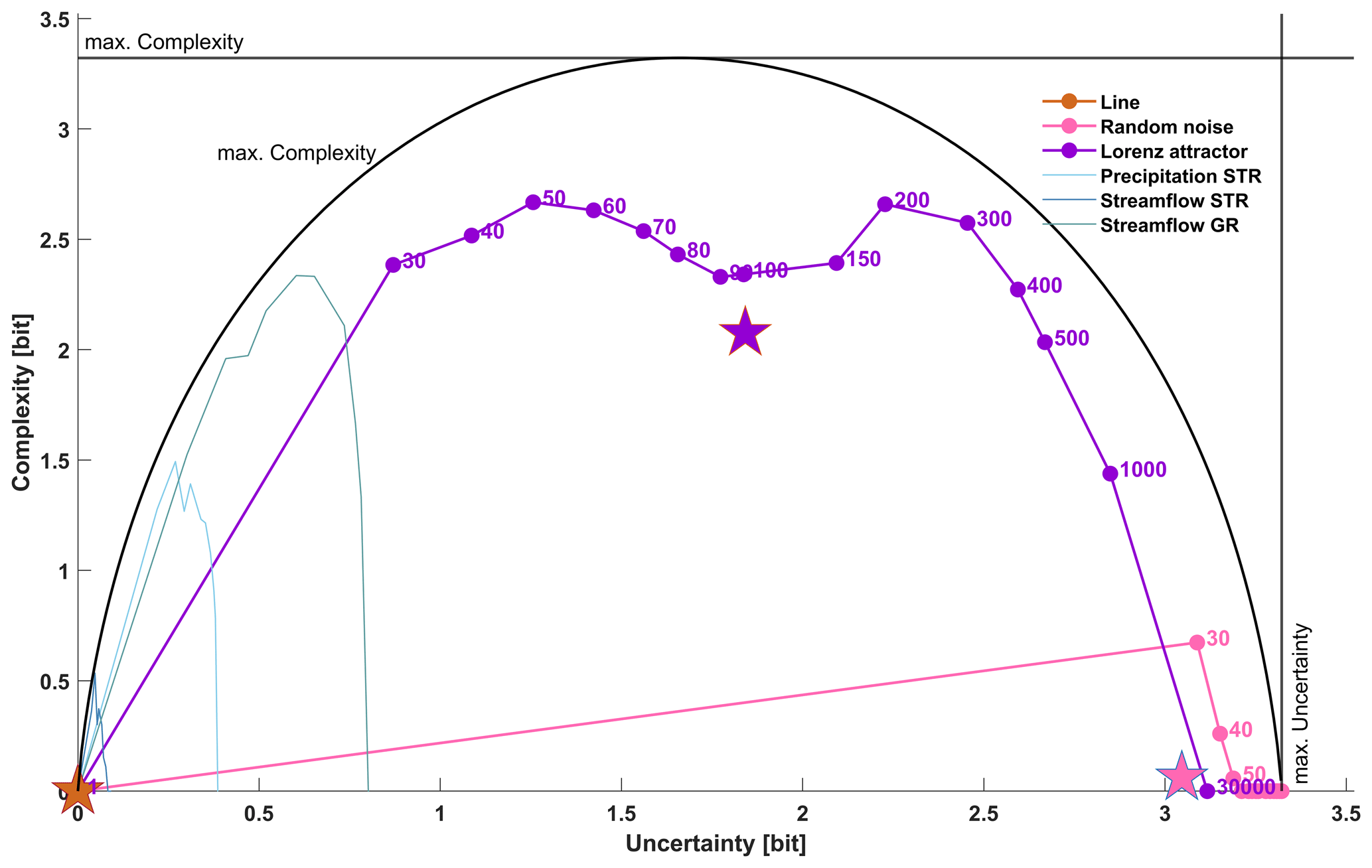
Figure 2The c-u-curves for synthetic (dotted) and hydro-meteorological (no marker) time series as shown in Fig. 1. The time series length is 30 000 for the synthetic data and 12 418 for the hydro-meteorological data. The number of value bins and entropy bins is 10, and the maximum uncertainty limit and maximum complexity limit are at log 2(10)=3.32 bits. The black arch shows the maximum complexity limit as a function of uncertainty. For the synthetic series, dot labels indicate the time slice width sw used to calculate uncertainty and complexity, and the pentagram positions indicate the mean uncertainty and mean complexity across all the chosen time-slicing schemes. The hydro-meteorological series are included to indicate their position within the full range of uncertainty and complexity; their details are shown in Fig. 3. For interpretations of the axis unit “bit”, see Sect. 2.1. The lines connecting individual c-u-curve points were included for better visibility and should not be interpreted as an indication of the guaranteed continuity of a c-u-curve.
Table 1Key characteristics of the c-u-curve for both the synthetic and hydro-meteorological time series.
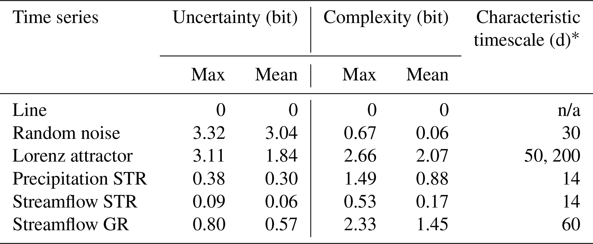
* Width of the time slice at which maximum complexity occurs.
n/a = not applicable
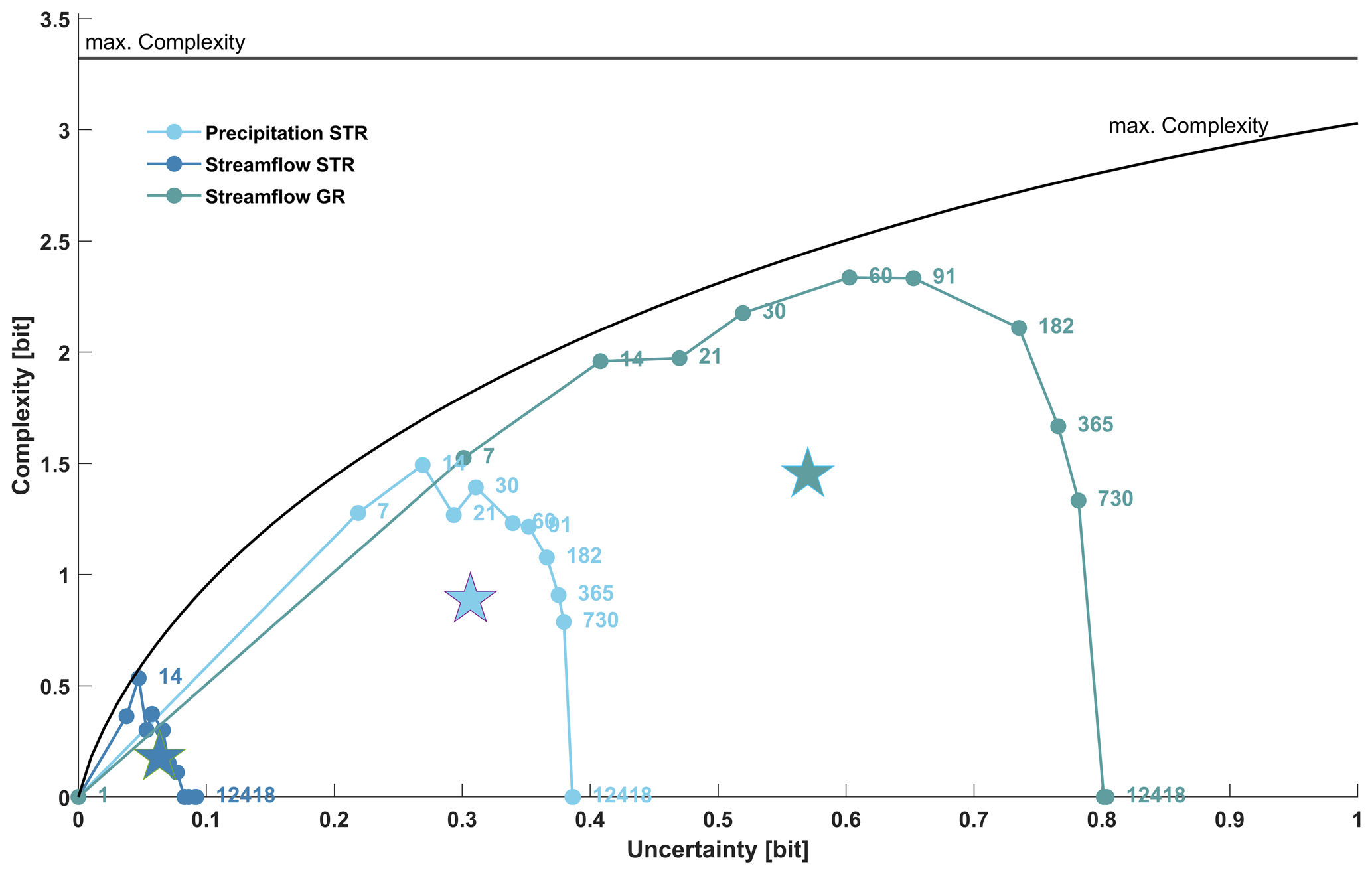
Figure 3The c-u-curve for all hydro-meteorological time series as shown in Fig. 1d–f. All the time series comprise 12 418 time steps, the number of value bins and entropy bins is 10, and the maximum uncertainty limit and maximum complexity limit are at log 2(10)=3.32 bits. The black arch shows the maximum complexity limit as a function of uncertainty. Note that for better display of details this is a horizontally zoomed-in version of Fig. 2. Dot labels indicate the time slice width sw used to calculate uncertainty and complexity. The pentagram positions indicate the mean uncertainty and mean complexity across all the chosen time-slicing schemes. For interpretations of the axis units “bit”, see Sect. 2.1. The lines connecting individual c-u-curve points were included for better visibility and should not be interpreted as an indication of the guaranteed continuity of a c-u-curve.
The overall shape of each c-u-curve contains key characteristics of the underlying time series. We start by discussing the c-u-curve plot of the straight line in Fig. 2. It shows – as expected – the simplest behaviour: for all the time-slicing schemes, both within-slice variability and across-slice variability are zero; i.e. the series displays zero uncertainty and complexity throughout (all dots are stacked at the origin). As a consequence, mean uncertainty and complexity across all the time-slicing schemes (indicated by the brown pentagram in the plot and listed in Table 1) are also zero.
The random noise series in Fig. 2 by contrast displays very high uncertainty and low complexity for most of the time-slicing schemes (most dots are stacked in the lower-right corner of the plot), and only for many but narrow time slices of 50, 40 and 30 values per slice does complexity assume non-zero values. This can be attributed to random effects in small samples, where purely by chance both highly and hardly variable samples can occur, thus creating a wide range of time slice entropies and resulting in apparent non-zero complexity. For wider slices, the larger sample size leads to more similarly distributed samples, resulting in a narrow range of time slice entropies and hence low complexity. Overall, mean uncertainty is very high and mean complexity is very low (position of the pink pentagram in Fig. 2 and values in Table 1), which is what we expected from random noise.
The Lorenz attractor in Fig. 2 reveals a more diverse behaviour across the range of time-slicing schemes. We start discussing it for the case of sw=30 000, i.e. when a single time slice covers the entire time series. As described in the general properties, for this case uncertainty is always at its maximum and equals the entropy of the time series, and complexity is zero, because only a single entropy value populates the entropy distribution. The actual uncertainty value (3.11 bits), or its distance from the upper limit of uncertainty (), is a key characteristic of the time series and expresses its overall variability. Decreasing the time slice width sw decreases within-slice variability (uncertainty). Also, it provides the potential for non-zero complexity as more and more entropy values populate the entropy distribution. For the curve shown in Fig. 2, complexity continuously increases and reaches its first maximum value of 2.66 bits (or ) for sw=200 and at 2.22 bits of uncertainty. This point is another key characteristic of a c-u-curve, indicating at which temporal aggregation the across-slice variability is highest. Further decreasing slice width first leads to a decrease and then another increase in complexity until a second maximum of 2.66 bits is reached at sw=50 (see the values in Table 1). Afterwards, complexity and uncertainty decrease to zero for sw=1, which is a general property of any c-u-curve (see the discussion of general properties above). Taking the uncertainty and complexity mean across all the time slices summarizes the c-u-curve in a single point (purple pentagram in Fig. 2, values in Table 1). For the Lorenz attractor, this reveals medium average uncertainty and high average complexity. In fact, the overall shape of the c-u-curve is close to the upper complexity limit reachable at a given uncertainty (shown in the plot as a black arch). This is in accordance with expectations, as the Lorenz attractor is known for exhibiting complex behaviour on many timescales. Interestingly, apart from revealing its generally complex behaviour, the c-u-curve also reveals at which particular time slice width the complexity of the Lorenz attractor is at a maximum. This can be interpreted as a “characteristic timescale” of the time series.
Next, we discuss the c-u-curves of the hydro-meteorological time series. In Fig. 2, they are indicated by the lines without markers. It is immediately obvious that they all possess low uncertainty, much lower than the theoretical maximum (indicated by the vertical “maximum uncertainty” limit) and the random noise and also lower than the Lorenz attractor. This is in accordance with our expectations and a consequence of the typically high temporal autocorrelation of hydro-meteorological time series, which clearly separates them from purely random time series. For a better view of the details, we re-plotted the hydro-meteorological time series in a subregion of the uncertainty limits in Fig. 3, which we will refer to in the following.
Despite the generally low uncertainties, the precipitation STR time series in Fig. 3 displays considerable complexity (indicated overall by the c-u-curve being close to the upper complexity limit and for mean complexity by the relatively high pentagram position), which can be explained by the existence of meteorological regimes with different levels of precipitation variability, such as dry periods (low variability), periods with alternating dry and wet periods (high variability) and wet times with diverse precipitation amounts (high variability). The highest complexity occurs for a time slice width of sw=14 d, indicating that the greatest variability of within-slice precipitation variability occurs for 2-week periods.
Interestingly, the corresponding streamflow STR time series displays much lower mean and maximum values (see Table 1) for both uncertainty (within-slice variability) and complexity (across-slice variability). This is in accordance with the general hydrological understanding that in the absence of major carryover mechanisms, rainfall–runoff transformation in catchments is mainly by aggregation and convolution, thus reducing the variability of the precipitation signal. It is noteworthy that while this harmonizing effect changes uncertainty and complexity means and maxima, it does not affect the characteristic timescale. For both streamflow STR and precipitation STR, this is 2 weeks. This suggests that precipitation remains the main control of streamflow complexity despite the processes involved in rainfall–runoff transformation.
This is different for the second streamflow GR time series. Here, in addition to the above-mentioned rainfall–runoff transformation, precipitation is partly stored as snow and later released as streamflow by melting. The temporal pattern of snowmelt is not only governed by snow availability, i.e. the precipitation regime, but also by energy availability, i.e. the long-term radiation and temperature regime. Such additional, independent controls of hydrological function can add uncertainty and complexity to streamflow production. Compared to streamflow STR, both uncertainty and complexity are indeed much larger in terms of mean and maximum values, and they are even larger than the corresponding values for precipitation STR (compare the pentagram positions in Fig. 3 and the values in Table 1). The characteristic timescale of streamflow GR is 2–3 months (60–91 d). This is considerably longer than for streamflow STR and can be explained by the carryover effect of snow accumulation and snowmelt acting on timescales of the order of months rather than days or weeks. For further illustration of the c-u-curve method, selected histograms for streamflow GR are shown in Appendix A.
In this paper we presented a method to analyse and classify dynamical systems by the two key features uncertainty and complexity. After dividing the time series into a set of time slices, the Shannon information entropy is calculated for the data in each time slice. Uncertainty is then calculated as the mean entropy of all the time slices, complexity as the entropy of all the entropy values. Complexity thus expresses “uncertainty about uncertainty” in the time series. Calculating and plotting uncertainty and complexity for many time-slicing schemes yields the c-u-curve, with key characteristics mean and maximum uncertainty, mean and maximum complexity, and the characteristic timescale of the time series. The latter is defined as the time slice width at which maximum complexity occurs.
The c-u-curve method has several useful properties: independence from the units of the data (both uncertainty and complexity are expressed in bit), existence of upper and lower bounds for both uncertainty and complexity as a function of the chosen data resolution, and bounded behaviour when approaching the upper and lower limits of time slicing. For a single time slice containing all data, uncertainty equals the time series entropy and complexity is zero; for time slices containing single values, both uncertainty and complexity are zero. The c-u-curve method is applicable to single-variate and multivariate data sets as well as to deterministic and probabilistic value representations (ensemble data sets), making it suitable for a wide range of tasks and systems. The main limitation of the method arises from the requirement of sufficiently populating distributions, which sets bounds on both the minimum and maximum widths of time slices.
We provided a proof of concept with the example of six time series, three of them artificial, three of them from hydro-meteorological observations. The artificial time series (straight line, random noise, Lorenz attractor) were chosen for their very different, exemplary and well-known behaviour and with the goal of demonstrating that the c-u-curve successfully reveals this behaviour, i.e. to demonstrate the general applicability of the method across a wide range of time series types. The observed time series (precipitation and streamflow from a mainly rainfall-dominated basin and streamflow from a basin where additionally snow processes influence the hydrological function) were chosen with the goal of demonstrating that the c-u-curve method reveals characteristics of real-world time series that are in accordance with the general knowledge of hydrological system functioning. For all the time series, we were able to show that the c-u-curve properties were distinctly different among the time series – which indicates that the method has discriminative capabilities useful for system classification and that the properties are in accordance with expectations based on system understanding. This indicates that the method captures relevant time series properties and expresses them in terms of uncertainty and complexity.
While the range of applications presented in this paper is small and mainly intended as a proof of concept, the results encourage further studies. Particularly for hydro-meteorological applications, we suggest that the c-u-curve method can be used for hydrological classification, as an objective function in hydrological model training, and for hydrological system analysis. For classification, we suggest using large hydro-meteorological data sets such as those from Addor et al. (2017) or Kuentz et al. (2017) to analyse whether the c-u-curve distinguishes between catchments with known differences, such as groundwater- and interflow-dominated, pristine and regulated, snow-free and snow-influenced, and arid and humid. In the same context, classifications by the c-u-curve can be compared to existing hydrological classifiers and signatures (such as the flow-duration curve and others as discussed in Jehn et al., 2020, Addor et al., 2018, and Kuentz et al., 2017) in terms of classification similarity and strength. The clear differences in c-u-curve properties between the two streamflow time series investigated in this paper encourage further research in this direction. In terms of hydrological model training, we suggest that the c-u-curve and its characteristic values can be used as an additional objective function. While standard hydrological objective functions such as Nash–Sutcliffe efficiency guide models towards point-by-point agreement of model output and observations, c-u-curve characteristics can guide models towards correct representations of short- and long-term variability patterns. Supported by the (dis-)similarities of the c-u-curve properties of the precipitation and streamflow time series presented in this paper, we also suggest that by analysing and comparing c-u-curve properties of input, internal states and output of hydrological systems, valuable insights into the functioning of these systems can be gained, e.g. whether they increase or decrease the uncertainty and complexity of the signals propagating through them. Further work on these topics is in progress. Finally, we propose the combination of the multiscale entropy (MSE) and c-u-curve approaches as discussed in Sect. 2.3 as a very promising avenue for future work.
As an illustration of how time series values within a time slice translate into histograms and entropy values, we show, for streamflow GR, in Fig. A1 the streamflow hydrographs and the corresponding histograms for three time slices. All the time slices have a width of 60 d, which is the slice width for which the series shows the highest complexity (compare Table 1 and Fig. 3). Overall, the time series (12 418 time steps) splits into time slices. For each slice, we calculated entropy and selected three interesting ones: one with the smallest of all entropy values (0 bits), one with the highest of all entropy values (2.27 bits), and one with an entropy of 0.61 bits, which is close to the overall mean entropy of 0.60 bits of all 206 time slices (“uncertainty”). The normalized time series of the three 60 d slices are shown in Fig. A1a–c, and the corresponding histograms are shown in Fig. A1d–f. As can be seen from Fig. A1a–c, for streamflow GR the possible range of variability within 60 d time slices is quite high, ranging from almost uniform flow (Fig. A1a) to time slices including very variable flow with both high-flow and low-flow conditions (Fig. A1c). This is summarized in Fig. A2, which shows the histogram of all 206 entropy values. Its entropy (“complexity”) is 2.33 bits (compare Table 1).
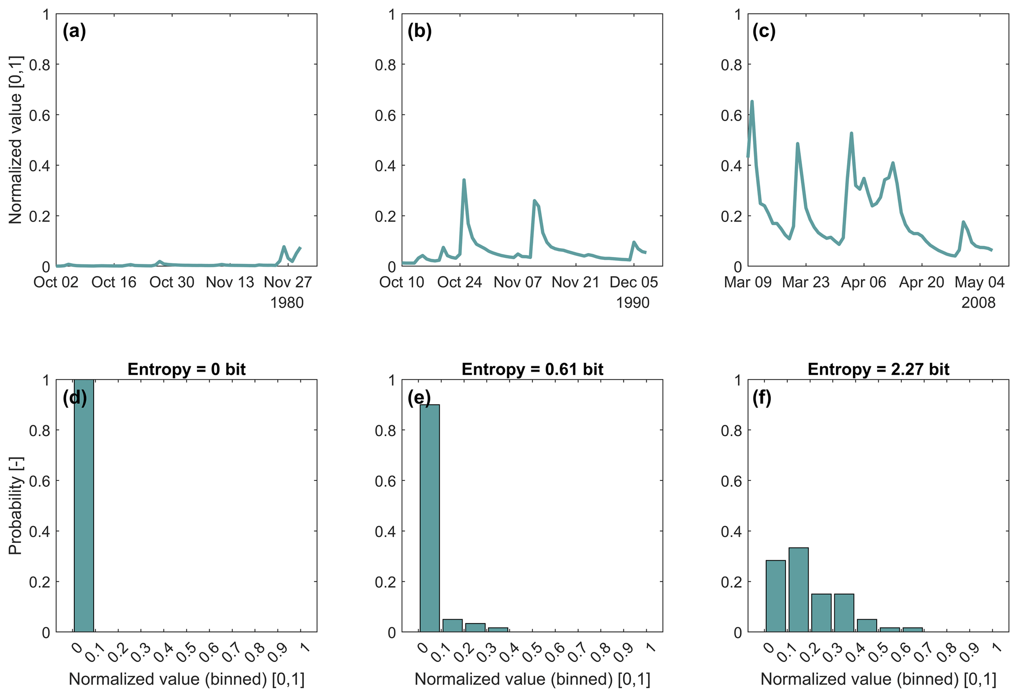
Figure A1Normalized streamflow hydrographs and corresponding histograms of three time slices from time series streamflow GR. Each time slice comprises 60 d. For the histograms, the value range of the normalized streamflow was split into 10 bins of uniform width. Subplots (a) and (d): time slice 2 October–30 November 1980, entropy=0 bits. Subplots (b) and (e): time slice 10 October–8 December 1990, entropy=0.61 bits. Subplots (c) and (f): time slice 9 March–7 May 2008, entropy=2.27 bits.
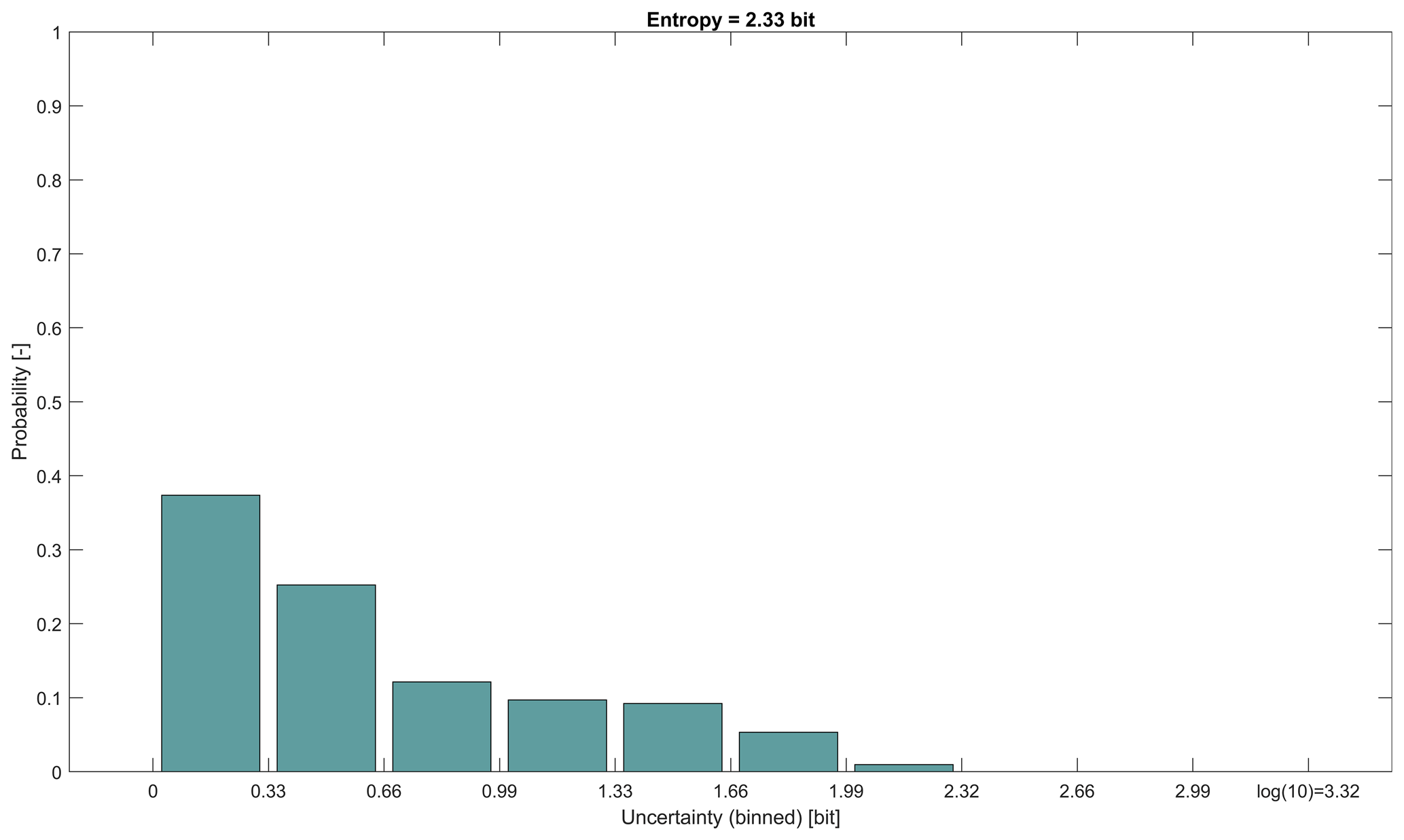
Figure A2Histogram of entropies from normalized time series streamflow GR split into 206 time slices, each with a width of 60 d. The entropy for each time slice was calculated from histograms (see Fig. A1). For the histogram, the possible range of entropy values ( bits) was split into 10 bins of uniform width. The entropy of this histogram of entropies is 2.33 bits (compare Table 1).
For the convenience of the reader, we repeat Theorem 5.12 from Conrad (2022) here and some related explanation in slightly modified and shortened form, but for the full proof, the reader is referred to the original publication. In the following, refers to a finite set of discrete, distinguishable states of a (physical) system, with the corresponding energy states and probabilities {p1,…pn} of the system being in a particular state. For each probability distribution p on S, the corresponding expected value of E is given by Eq. (B1).
This number is between minEj and maxEj. For a chosen (a priori known) value of , the goal is to find the probability distribution q with the given and maximum entropy. For the general case when q is not a uniform distribution, Theorem 5.12 provides a semi-analytical solution.
Theorem 5.12. If the Ej values are not all equal, then, for each between minEj and maxEj, there is a unique probability distribution q on {s1,…sn} satisfying the condition and having maximum entropy. It is given by the formula
for a unique extended real number β in that depends on . In particular, corresponds to , β=∞ corresponds to , and β=0 (the uniform distribution) corresponds to the arithmetic mean , so β>0 when and β<0 when . The value of β can be numerically approximated with an iterative algorithmic recipe and Eqs. (B1) and (B2) (see example 5.14 in Conrad, 2022).
The code and data used to conduct all the analyses in this paper are publicly available at https://doi.org/10.5281/zenodo.7276917 (Ehret, 2022).
UE developed the c-u-curve method and wrote all the related code. UE and PD designed the study together and wrote the manuscript together.
The contact author has declared that neither of the authors has any competing interests.
Publisher's note: Copernicus Publications remains neutral with regard to jurisdictional claims in published maps and institutional affiliations.
We gratefully acknowledge support by the Deutsche Forschungsgemeinschaft (DFG) and the Open Access Publishing Fund of the Karlsruhe Institute of Technology (KIT). We thank Philipp Reiser from the University of Stuttgart for pointing us to Conrad (2022).
This research has been supported by the INSPIRE Faculty Fellowship, Department of Science and Technology, Government of India (grant no. DST/INSPIRE/04/2022/001952, Faculty Registration No.: IFA22-EAS 114).
The article processing charges for this open-access publication were covered by the Karlsruhe Institute of Technology (KIT).
This paper was edited by Jim Freer and reviewed by Jasper Vrugt and one anonymous referee.
Addor, N., Newman, A. J., Mizukami, N., and Clark, M. P.: The CAMELS data set: catchment attributes and meteorology for large-sample studies, Hydrol. Earth Syst. Sci., 21, 5293–5313, https://doi.org/10.5194/hess-21-5293-2017, 2017.
Addor, N., Nearing, G., Prieto, C., Newman, A. J., Le Vine, N., and Clark, M. P.: A Ranking of Hydrological Signatures Based on Their Predictability in Space, Water Resour. Res., 54, 8792–8812, https://doi.org/10.1029/2018WR022606, 2018.
Azmi, E., Ehret, U., Weijs, S. V., Ruddell, B. L., and Perdigão, R. A. P.: Technical note: “Bit by bit”: a practical and general approach for evaluating model computational complexity vs. model performance, Hydrol. Earth Syst. Sci., 25, 1103–1115, https://doi.org/10.5194/hess-25-1103-2021, 2021.
Bossel, H.: Dynamics of forest dieback: Systems analysis and simulation, Ecol. Model., 34, 259–288, https://doi.org/10.1016/0304-3800(86)90008-6, 1986.
Bossel, H.: Systems and Models. Complexity, Dynamics, Evolution, Sustainability, Books on Demand GmbH, Norderstedt, Germany, 372 pp., ISBN 978-3-8334-8121-5, 2007.
Bras, R. L.: Complexity and organization in hydrology: A personal view, Water Resour. Res., 51, 6532–6548, https://doi.org/10.1002/2015wr016958, 2015.
Brunsell, N. A.: A multiscale information theory approach to assess spatial–temporal variability of daily precipitation, J. Hydrol., 385, 165–172, https://doi.org/10.1016/j.jhydrol.2010.02.016, 2010.
Castillo, A., Castelli, F., and Entekhabi, D.: An entropy-based measure of hydrologic complexity and its applications, Water Resour. Res., 51, 5145–5160, https://doi.org/10.1002/2014wr016035, 2015.
Chou, C.-M.: Wavelet-Based Multi-Scale Entropy Analysis of Complex Rainfall Time Series, Entropy, 13, 241–253, 2011.
Conrad, K.: Probability distributions and maximum entropy, https://kconrad.math.uconn.edu/blurbs/analysis/entropypost.pdf, last access: 30 October 2022.
Costa, M., Goldberger, A. L., and Peng, C. K.: Multiscale Entropy Analysis of Complex Physiologic Time Series, Phys. Rev. Lett., 89, 068102, https://doi.org/10.1103/PhysRevLett.89.068102, 2002.
Costa, M., Goldberger, A. L., and Peng, C. K.: Multiscale entropy analysis of biological signals, Phys. Rev. E, 71, 021906, https://doi.org/10.1103/PhysRevE.71.021906, 2005.
Cover, T. and Thomas, J. A.: Elements of Information Theory, Wiley Series in Telecommunications and Signal Processing, Wiley-Interscience, https://doi.org/10.1002/0471200611, 2006.
Dey, P. and Mujumdar, P.: On the statistical complexity of streamflow, Hydrol. Sci. J., 67, 40–53, https://doi.org/10.1080/02626667.2021.2000991, 2022.
Dooge, J. C. I.: Looking for hydrologic laws, Water Resour. Res., 22, 46S–58S, https://doi.org/10.1029/WR022i09Sp0046S, 1986.
Ehret, U.: KIT-HYD/c-u-curve: Version 1.1 (1.1.0), Zenodo [code/data], https://doi.org/10.5281/zenodo.7276917, 2022.
Ehret, U., Gupta, H. V., Sivapalan, M., Weijs, S. V., Schymanski, S. J., Blöschl, G., Gelfan, A. N., Harman, C., Kleidon, A., Bogaard, T. A., Wang, D., Wagener, T., Scherer, U., Zehe, E., Bierkens, M. F. P., Di Baldassarre, G., Parajka, J., van Beek, L. P. H., van Griensven, A., Westhoff, M. C., and Winsemius, H. C.: Advancing catchment hydrology to deal with predictions under change, Hydrol. Earth Syst. Sci., 18, 649–671, https://doi.org/10.5194/hess-18-649-2014, 2014.
Engelhardt, S., Matyssek, R., and Huwe, B.: Complexity and information propagation in hydrological time series of mountain forest catchments, Eur. J. For. Res., 128, 621–631, https://doi.org/10.1007/s10342-009-0306-2, 2009.
Feldman, D. P. and Crutchfield, J. P.: Measures of statistical complexity: Why?, Phys. Lett. A, 238, 244–252, https://doi.org/10.1016/s0375-9601(97)00855-4, 1998.
Forrester, J. W.: Principles of Systems, 2nd edn., Productivity Press, Portland, OR, 391 pp., ISBN 978-1883823412, 1968.
Freedman, D. and Diaconis, P.: On the histogram as a density estimator: L2 theory, Z. Wahrscheinlichkeit., 57, 453–476, https://doi.org/10.1007/BF01025868, 1981.
Gell-Mann, M.: What is complexity? Remarks on simplicity and complexity by the Nobel Prize-winning author of The Quark and the Jaguar, Complexity, 1, 16–19, https://doi.org/10.1002/cplx.6130010105, 1995.
Guzmán-Vargas, L., Ramírez-Rojas, A., and Angulo-Brown, F.: Multiscale entropy analysis of electroseismic time series, Nat. Hazards Earth Syst. Sci., 8, 855–860, https://doi.org/10.5194/nhess-8-855-2008, 2008.
Hastings, A., Hom, C. L., Ellner, S., Turchin, P., and Godfray, H. C. J.: Chaos in Ecology – Is Mother Nature a Strange Attractor?, Annu. Rev. Ecol. Syst., 24, 1–33, 1993.
Hauhs, M. and Lange, H.: Classification of Runoff in Headwater Catchments: A Physical Problem?, Geography Compass, 2, 235–254, https://doi.org/10.1111/j.1749-8198.2007.00075.x, 2008.
Jakeman, A. J. and Hornberger, G. M.: How much complexity is warranted in a rainfall-runoff model?, Water Resour. Res., 29, 2637–2649, https://doi.org/10.1029/93WR00877, 1993.
Jehn, F. U., Bestian, K., Breuer, L., Kraft, P., and Houska, T.: Using hydrological and climatic catchment clusters to explore drivers of catchment behavior, Hydrol. Earth Syst. Sci., 24, 1081–1100, https://doi.org/10.5194/hess-24-1081-2020, 2020.
Jenerette, G. D., Barron-Gafford, G. A., Guswa, A. J., McDonnell, J. J., and Villegas, J. C.: Organization of complexity in water limited ecohydrology, Ecohydrology, 5, 184–199, https://doi.org/10.1002/eco.217, 2012.
Jovanovic, T., Garcia, S., Gall, H., and Mejia, A.: Complexity as a streamflow metric of hydrologic alteration, Stoch. Env. Res. Risk A., 31, 2107–2119, https://doi.org/10.1007/s00477-016-1315-6, 2017.
Knuth, K. H.: Optimal data-based binning for histograms and histogram-based probability density models, Digit. Signal Process., 95, 102581, https://doi.org/10.1016/j.dsp.2019.102581, 2019.
Koutsoyiannis, D.: On the quest for chaotic attractors in hydrological processes, Hydrolog. Sci. J., 51, 1065–1091, https://doi.org/10.1623/hysj.51.6.1065, 2006.
Kuentz, A., Arheimer, B., Hundecha, Y., and Wagener, T.: Understanding hydrologic variability across Europe through catchment classification, Hydrol. Earth Syst. Sci., 21, 2863–2879, https://doi.org/10.5194/hess-21-2863-2017, 2017.
Ladyman, J., Lambert, J., and Wiesner, K.: What is a complex system?, Eur. J. Philos. Sci., 3, 33–67, https://doi.org/10.1007/s13194-012-0056-8, 2013.
Li, Z. and Zhang, Y.-K.: Multi-scale entropy analysis of Mississippi River flow, Stoch. Env. Res. Risk A., 22, 507–512, https://doi.org/10.1007/s00477-007-0161-y, 2008.
Liu, Y. and Gupta, H. V.: Uncertainty in hydrologic modeling: Toward an integrated data assimilation framework, Water Resour. Res., 43, W07401, https://doi.org/10.1029/2006WR005756, 2007.
Lloyd, S.: Measures of complexity: a nonexhaustive list, IEEE Contr. Syst. Mag., 21, 7–8, https://doi.org/10.1109/MCS.2001.939938, 2001.
LopezRuiz, R., Mancini, H. L., and Calbet, X.: A statistical measure of complexity, Phys. Lett. A, 209, 321–326, https://doi.org/10.1016/0375-9601(95)00867-5, 1995.
Lorenz, E. N.: Deterministic Nonperiodic Flow, J. Atmos. Sci., 20, 130–141, https://doi.org/10.1175/1520-0469(1963)020<0130:Dnf>2.0.Co;2, 1963.
Lorenz, E. N.: Predictability of a flow which possesses many scales of motion, Tellus, 21, 289–308, 1969.
Moiseev, I.: Lorenz attractor plot, MATLAB Central File Exchange, https://www.mathworks.com/matlabcentral/fileexchange/30066-lorenz-attaractor-plot, retrieved: 3 January 2022.
Moriasi, D. N., Arnold, J. G., Van Liew, M. W., Bingner, R. L., Harmel, R. D., and Veith, T. L.: Model evaluation guidelines for systematic quantification of accuracy in watershed simulations, T. ASABE, 50, 885–900, https://doi.org/10.13031/2013.23153, 2007.
Neuper, M. and Ehret, U.: Quantitative precipitation estimation with weather radar using a data- and information-based approach, Hydrol. Earth Syst. Sci., 23, 3711–3733, https://doi.org/10.5194/hess-23-3711-2019, 2019.
Newman, A. J., Clark, M. P., Sampson, K., Wood, A., Hay, L. E., Bock, A., Viger, R. J., Blodgett, D., Brekke, L., Arnold, J. R., Hopson, T., and Duan, Q.: Development of a large-sample watershed-scale hydrometeorological data set for the contiguous USA: data set characteristics and assessment of regional variability in hydrologic model performance, Hydrol. Earth Syst. Sci., 19, 209–223, https://doi.org/10.5194/hess-19-209-2015, 2015.
Ombadi, M., Nguyen, P., Sorooshian, S. and Hsu, K.: Complexity of hydrologic basins: A chaotic dynamics perspective, J. Hydrol., 597, 126222, https://doi.org/10.1016/j.jhydrol.2021.126222, 2021.
Ossola, A., Hahs, A. K., and Livesley, S. J.: Habitat complexity influences fine scale hydrological processes and the incidence of stormwater runoff in managed urban ecosystems, J. Environ. Manage., 159, 1–10, https://doi.org/10.1016/j.jenvman.2015.05.002, 2015.
Pachepsky, Y., Guber, A., Jacques, D., Simunek, J., Van Genuchten, M. T., Nicholson, T., and Cady, R.: Information content and complexity of simulated soil water fluxes, Geoderma, 134, 253–266, https://doi.org/10.1016/j.geoderma.2006.03.003, 2006.
Pande, S. and Moayeri, M.: Hydrological Interpretation of a Statistical Measure of Basin Complexity, Water Resour. Res., 54, 7403–7416, https://doi.org/10.1029/2018wr022675, 2018.
Pechlivanidis, I. G., Jackson, B., McMillan, H., and Gupta, H. V.: Robust informational entropy-based descriptors of flow in catchment hydrology, Hydrolog. Sci. J., 61, 1–18, https://doi.org/10.1080/02626667.2014.983516, 2016.
Phillips, J. D.: Deterministic chaos and historical geomorphology: A review and look forward, Geomorphology, 76, 109–121, https://doi.org/10.1016/j.geomorph.2005.10.004, 2006.
Prokopenko, M., Boschetti, F., and Ryan, A. J.: An information-theoretic primer on complexity, self-organization, and emergence, Complexity, 15, 11–28, https://doi.org/10.1002/cplx.20249, 2009.
Sawicz, K., Wagener, T., Sivapalan, M., Troch, P. A., and Carrillo, G.: Catchment classification: empirical analysis of hydrologic similarity based on catchment function in the eastern USA, Hydrol. Earth Syst. Sci., 15, 2895–2911, https://doi.org/10.5194/hess-15-2895-2011, 2011.
Scott, D. W.: On optimal and data-based histograms, Biometrika, 66, 605–610, https://doi.org/10.1093/biomet/66.3.605, 1979.
Seibert, S. P., Jackisch, C., Ehret, U., Pfister, L., and Zehe, E.: Unravelling abiotic and biotic controls on the seasonal water balance using data-driven dimensionless diagnostics, Hydrol. Earth Syst. Sci., 21, 2817–2841, https://doi.org/10.5194/hess-21-2817-2017, 2017.
Shannon, C. E.: A mathematical theory of communication, Bell Syst. Tech. J., 27, 623–656, 1948.
Singh, V. P.: Entropy Theory and its Application in Environmental and Water Engineering, John Wiley & Sons, Ltd, https://doi.org/10.1002/9781118428306, 2013.
Sivakumar, B. and Singh, V. P.: Hydrologic system complexity and nonlinear dynamic concepts for a catchment classification framework, Hydrol. Earth Syst. Sci., 16, 4119–4131, https://doi.org/10.5194/hess-16-4119-2012, 2012.
Sivakumar, B., Jayawardena, A. W., and Li, W. K.: Hydrologic complexity and classification: a simple data reconstruction approach, Hydrol. Process., 21, 2713–2728, https://doi.org/10.1002/hyp.6362, 2007.
Strogatz, S. H.: Nonlinear Dynamics and Chaos: With applications to Physics, Biology, Chemistry and Engineering, Addison-Wesley Publishing Company, Reading, MA, 498 pp., https://doi.org/10.1201/9780429492563, 1994.
Sturges, H. A.: The Choice of a Class Interval, J. Am. Stat. Assoc., 21, 65–66, https://doi.org/10.1080/01621459.1926.10502161, 1926.
Vrugt, J. A., Gupta, H. V., Bouten, W., and Sorooshian, S.: A Shuffled Complex Evolution Metropolis algorithm for optimization and uncertainty assessment of hydrologic model parameters, Water Resour. Res., 39, 1201, https://doi.org/10.1029/2002WR001642, 2003.
Vrugt, J. A., ter Braak, C. J. F., Gupta, H. V., and Robinson, B. A.: Equifinality of formal (DREAM) and informal (GLUE) Bayesian approaches in hydrologic modeling?, Stoch. Env. Res. Risk A., 23, 1011–1026, https://doi.org/10.1007/s00477-008-0274-y, 2009.
Wagener, T., Sivapalan, M., Troch, P., and Woods, R.: Catchment Classification and Hydrologic Similarity, Geography Compass, 1, 901–931, https://doi.org/10.1111/j.1749-8198.2007.00039.x, 2007.
Wu, S.-D., Wu, C.-W., Lin, S.-G., Wang, C.-C., and Lee, K.-Y.: Time Series Analysis Using Composite Multiscale Entropy, Entropy, 15, 1069–1084, 2013.
Yapo, P. O., Gupta, H. V., and Sorooshian, S.: Multi-objective global optimization for hydrologic models, J. Hydrol., 204, 83–97, https://doi.org/10.1016/s0022-1694(97)00107-8, 1998.
Zhou, Y., Zhang, Q., Li, K., and Chen, X. H.: Hydrological effects of water reservoirs on hydrological processes in the East River (China) basin: complexity evaluations based on the multi-scale entropy analysis, Hydrol. Process., 26, 3253–3262, https://doi.org/10.1002/hyp.8406, 2012.
- Abstract
- Introduction
- Method
- Application to synthetic and real-world time series
- Summary and conclusions
- Appendix A: Histograms for time series streamflow GR
- Appendix B: Proof of the existence of an upper bound of the c-u-curve
- Code and data availability
- Author contributions
- Competing interests
- Disclaimer
- Acknowledgements
- Financial support
- Review statement
- References
c-u-curvemethod to characterize dynamical (time-variable) systems of all kinds.
Uis for uncertainty and expresses how well a system can be predicted in a given period of time.
Cis for complexity and expresses how predictability differs between different periods, i.e. how well predictability itself can be predicted. The method helps to better classify and compare dynamical systems across a wide range of disciplines, thus facilitating scientific collaboration.
c-u-curvemethod to characterize dynamical (time-variable) systems of all kinds....
- Abstract
- Introduction
- Method
- Application to synthetic and real-world time series
- Summary and conclusions
- Appendix A: Histograms for time series streamflow GR
- Appendix B: Proof of the existence of an upper bound of the c-u-curve
- Code and data availability
- Author contributions
- Competing interests
- Disclaimer
- Acknowledgements
- Financial support
- Review statement
- References