The precision of satellite-based net irrigation quantification in the Indus and Ganges basins

Even though irrigation is the largest direct anthropogenic interference in the natural terrestrial water cycle, limited knowledge of the amount of water applied for irrigation exists. Quantification of irrigation via evapotranspiration (ET) or soil moisture residuals between remote-sensing models and hydrological models, with the latter acting as baselines without the influence of irrigation, have successfully been applied in various regions. Here, we implement a novel ensemble methodology to estimate the precision of ET-based net irrigation quantification by combining different ET and precipitation products in the Indus and Ganges basins. A multi-model calibration of 15 models independently calibrated to simulate rainfed ET was conducted before the irrigation quantification. Based on the ensemble average, the 2003–2013 net irrigation amounts to 233 mm yr⁻¹ (74 km³ yr⁻¹) and 101 mm yr⁻¹ (67 km³ yr⁻¹) in the Indus and Ganges basins, respectively. Net irrigation in the Indus Basin is evenly split between dry and wet periods, whereas 70 % of net irrigation occurs during the dry period in the Ganges Basin. We found that, although annual ET from remote-sensing models varied by 91.5 mm yr⁻¹, net irrigation precision was within 25 mm per season during the dry period for the entire study area, which emphasizes the robustness of the applied multi-model calibration approach. Net irrigation variance was found to decrease as ET uncertainty decreased, which is related to the climatic conditions, i.e., high uncertainty under arid conditions. A variance decomposition analysis showed that ET uncertainty accounted for 73 % of the overall net irrigation variance and that the influence of precipitation uncertainty was seasonally dependent, i.e., with an increase during the monsoon season. The results underline the robustness of the framework to support large-scale sustainable water resource management of irrigated land.

1 Introduction

A total of 40 % of global irrigated cropland is sustained by groundwater abstraction (Siebert et al., 2010); this has caused regional groundwater levels to decline, as abstraction rates have exceeded the annual recharge (Ahmad et al., 2021; Malakar et al., 2021; Rodell et al., 2009; Shekhar et al., 2020). By 2050, global food production will have to increase by 60 % to meet global food demand, and 90 % of this increase in food production is projected to take place in developing countries (Alexandratos and Bruinsma, 2012). Thus, water scarcity is likely to intensify and threaten the livelihood of millions of people living in the affected areas as well as global food security (Jain et al., 2021).

Despite this, our knowledge of the extent of irrigated areas and irrigated water use is limited. In recent years, mapping of irrigated areas from microwave and/or optical satellite data has advanced (Bazzi et al., 2021; Dari et al., 2021; Lawston et al., 2017; Sharma et al., 2021), and scientific advances have aimed at estimating irrigation water use by isolating satellite-based ET or soil moisture as a non-precipitation source (Brocca et al., 2018; Jalilvand et al., 2019, 2021; Koch et al., 2020; Zaussinger et al., 2019; Zohaib and Choi, 2020). Knowledge of irrigated water use is important for correct modeling of the water balance (Shah et al., 2021, 2019a, b; Soni and Syed, 2021) and modeling of regional climate, which can be significantly modulated by irrigation (Mishra et al., 2020; Thiery et al., 2020). Ultimately, such improved knowledge will support policymakers with respect to reaching valid and timely decisions on water management (Schwartz et al., 2020).

Soil-moisture-based irrigation estimates have been found to yield irrigation approximations with satisfactory accuracy (Brocca et al., 2018; Dari et al., 2020; Zaussinger et al., 2019). However, the advantages of using ET over soil moisture are as follows: (1) ET is directly linked to plant transpiration reacting to irrigation, whereas soil moisture produces an indirect estimate, especially as many remote-sensing systems only penetrate the topsoil (a few centimeters); (2) the spatial resolution of readily available ET datasets (e.g., derived from optical and thermal MODIS data) is higher. In contrast, the disadvantage of using ET to estimate irrigation is as follows: the magnitude of the rainfed component of the products can vary substantially, which can, in theory, lead to diverging irrigation estimates when comparing across ET products. Also, cloud cover is a limitation, as it can affect the temporal resolution of the ET-based approach; we addressed this by aggregating the original datasets into monthly estimates. Similar to Koch et al. (2020), we used a hydrological model calibrated for rainfed conditions to simulate a rainfed baseline and, thus, accommodate for the differences between ET products.

Less attention has been paid to quantifying the uncertainty of ET-based irrigation estimates. Uncertainties can be expressed twofold: accuracy and precision. Accuracy captures how close the estimates are to observations, whereas precision investigates how close or dispersed estimates are with respect to each other. The accuracy of irrigation estimates can only be assessed by observations, which are commonly absent at the larger scale. In this study, we focus on precision, which can be addressed using an ensemble approach, utilizing multiple models, i.e., with different hydrometeorological datasets.

Although remote-sensing-based hydrometeorological data have the advantage of high spatial coverage, the inherent uncertainty in ET and precipitation products may arise from a variety of potential errors (e.g., different revisit times from satellite sensors and the model approach). The evaluation of evapotranspiration products by the water balance ET and Budyko ET approach in Africa and Europe have shown that ET remote-sensing products may differ substantially when comparing magnitude and/or spatial patterns (Stisen et al., 2021; Weerasinghe et al., 2020). The evaluation of precipitation products has, analogous to the ET products, shown that large differences in magnitude and spatial patterns are evident. For example, Yang and Luo (2014) evaluated the performance of three precipitation products over an arid region in China and found that corrections were necessary as the products yielded very different magnitudes and spatial patterns. Logah et al. (2021) found that the precipitation products generally performed better during the dry period and that the products had difficulties simulating high-intensity rainfall in the Black Volta Basin.

The current study area covers the Indus and Ganges basins, shared between more than a billion people in India, Pakistan, Nepal, Bangladesh, China, and Afghanistan. Large government investments in India in the 1960s have led the region, and mainly the state of Punjab, to be the largest area heavily equipped for irrigation at the global scale, through the construction of the Indus Basin and Bhakra irrigation systems, providing food security beyond its borders (Sharma et al., 2010). A rapidly growing population, combined with decreasing investment in irrigation infrastructure, has increased unsustainable groundwater use and resulted in a regional decline in the groundwater level (Rodell et al., 2009). A regional survey indicated that irrigation from groundwater was more widespread than first assumed, as only 5 % of surveyed villages consider their agricultural practice to be totally rainfed (Shah et al., 2006).

This study applies, for the first time, an ensemble approach to investigate the robustness of ET-based estimates of irrigation at a regional scale for a global hotspot of irrigation-induced groundwater overexploitation. In this way, previous work (Koch et al., 2020; Romaguera et al., 2014) is expanded by using different ET and precipitation products to quantify irrigation water use and precision of an ET-based framework. The three main objectives of this paper are as follows: (1) selecting and analyzing a suitable global ET and precipitation dataset for irrigation quantification over the Indus and Ganges basins, (2) building a hydrological model to simulate rainfed ET at a 5 km spatial resolution via a state-of-the-art calibration tool, and (3) evaluating the precision and influence of ET and precipitation uncertainties in the estimation of irrigation.

2 Study area

The Indus and Ganges basins extend over an area of 2.2×10⁶ km² (Fig. 1). The region can be subdivided into four geographical regions: (1) the Himalayan mountains along the northern boundary; (2) the Indo-Gangetic outwash plain; (3) the Thar Desert separating the two basins; and (4) the peninsular plateau south of the Indo-Gangetic Plain, characterized by highlands, valleys, and rounded hills. The climate is monsoon dominated and varies from a tropical humid zone in the eastern Ganges Basin and along the mountain range to an arid climate in the lower Indus Basin (see Fig. 1). Most precipitation occurs from July to September during the monsoon season and varies on average between 200 and 1200 mm yr⁻¹ (2000–2019) across the basins.

Figure 1 Map of climate zones from the Joint Research Center of the European Commission (Spinoni, 2015) and the area equipped for irrigation as a percentage of the total area (Siebert et al., 2013). The inset shows the location of the Indus and Ganges basins and rivers.

Agriculture accounts for 70 % of land cover in the basins. Summer rice and winter wheat rotation is the most common cropping system in the Indo-Gangetic Plain, mixed with cotton and sugarcane outside of the plain (Cai et al., 2010). Summer rice water requirements are generally met by precipitation during the wet period (May–November), except in the lower Indus Basin, which has precipitation rates of less than 50 mm per month, where extensive irrigation also takes place during the monsoon months. However, winter wheat heavily depends on irrigation across the entire region, as the average precipitation rate is less than 25 mm per month during the dry period (December–April).

3 Method and data

3.1 Hydrological model

This study applies the grid-based mesoscale Hydrological Model (mHM; Kumar et al., 2013; Samaniego et al., 2010; Thober et al., 2019), version 5.11.0 (Samaniego et al., 2021). mHM uses a multiscale parameter regionalization technique that links spatial distributions of model parameters at an intermediate scale, representing hydrological processes, to finer-scale variability in soil texture, topography, and vegetation via nonlinear transfer functions. The transfer functions have a limited number of global parameters that enable efficient calibration (Samaniego et al., 2017, 2021). The hydrological models set up for this study used 10 km gridded metrological forcing and 1 km morphological data, and they were calibrated and executed at a 5 km spatial resolution to simulate rainfed ET baselines, i.e., representing a purely rainfed hydrological system without the presence of irrigation.

For our model setup, actual ET is calculated by reducing potential ET using the Feddes soil water stress factor (Feddes et al., 1976) in combination with a root fraction distribution over the defined number of soil layers. mHM offers an option for dynamic downscaling of potential ET from the metrological resolution to the model resolution by incorporating vegetation dynamics from a monthly leaf area index (LAI) climatology (Demirel et al., 2018). To set up mHM to simulate rainfed ET, Koch et al. (2020) modified the LAI climatologies by removing the imprint of irrigation on vegetation dynamics by substituting the original LAI climatologies in irrigated areas with a mean LAI climatology from rainfed areas to simulate the rainfed ET baseline as a natural scenario. In this study, we used the original LAI climatologies without modifications to simulate the rainfed ET baselines under a managed scenario, as modification of LAI climatologies to natural conditions potentially overestimates net irrigation by underestimating rainfed ET over irrigated areas.

In this study, different precipitation products were used as forcing (as described in Sect. 3.3), the daily average air temperature was acquired from ERA-Land, and potential ET was calculated by using the FAO 56 Penman–Monteith equation with ECMWF reanalysis fifth-generation – enhanced resolution (ERA5-Land) variables (Muñoz Sabater, 2019). We chose the FAO 56 Penman–Monteith (PM) equation based on its documented ability to estimate potential ET used in irrigation management and comparative studies evaluating FAO 56 PM against other potential ET estimation methods (Allen et al., 1989; Jensen and Allen, 2016) The digital elevation model (DEM) was obtained from NASA's Shuttle Radar Topography Mission data (Jarvis et al., 2016). Soil texture information was processed for six horizons from the SoilGrids^TM database and resampled to 1 km using the mean function. LAI and land cover data were collected from MODIS MCD15A2H.v006 and MCD12Q1.v006, respectively.

3.2 Calibration and validation strategy

The calibration framework is designed to obtain hydrological models that simulate baselines of rainfed ET. The hydrological models used in this study were calibrated using the Pareto archived dynamically dimensioned search (PADDS) algorithm (Asadzadeh and Tolson, 2009) implemented in the OSTRICH Optimization Software Toolkit (Matott, 2017). The calibration was performed with 600 iterations and a perturbation size of 0.2. We calibrated 12 parameters that were identified based on a prior sensitivity analysis perturbing 1 parameter at a time and recording the change in the objective function. The OSTRICH algorithm provides the modeler with a Pareto front of dominant solutions, which enables the modeler to select the solutions that mark the most acceptable trade-off between multiple objective functions.

OSTRICH was used to minimize two objective functions that address the magnitude and seasonal spatial pattern of ET over rainfed cropland and naturally vegetated areas for the calibration period from 2003 to 2007. First, the monthly mean absolute error (MAE) is used to target the magnitude of ET over rainfed cropland.

$$\begin{array}{}\text{(1)}& \mathrm{MAE}={\displaystyle \frac{{\sum }_{i=\mathrm{1}}^n\left|x_i-y_i\right|}{n}},\end{array}$$

where x_i and y_i represent the respective observed and simulated ET at cell i, and n is the number of cells. MAE has an optimal value of zero and varies from zero to positive infinity. Second, optimization of the spatial ET pattern was targeted by applying the spatial efficiency (SPAEF) metric on ET in rainfed cropland and naturally vegetated areas for the mean dry and wet periods. SPAEF is a multicomponent bias-insensitive spatial pattern metric that evaluates the ability of the model to simulate the observed correlation, variance, and histogram (Demirel et al., 2018; Koch et al., 2018).

$$\begin{array}{c}\text{(2)}& {\displaystyle }\mathrm{SPAEF}=\mathrm{1}-\sqrt{(\mathit{\alpha }-\mathrm{1}{)}^{\mathrm{2}}+(\mathit{\beta }-\mathrm{1}{)}^{\mathrm{2}}+(\mathit{\gamma }-\mathrm{1}{)}^{\mathrm{2}}},{\displaystyle }\mathit{\alpha }=\mathit{\rho }(x,y),\mathit{\beta }=\left({\displaystyle \frac{{\mathit{\sigma }}_x}{{\mathit{\mu }}_x}}\right)/\left({\displaystyle \frac{{\mathit{\sigma }}_y}{{\mathit{\mu }}_y}}\right),\mathrm{and}\\ {\displaystyle }\mathit{\gamma }={\displaystyle \frac{{\sum }_{j=\mathrm{1}}^n\min (K_j,L_j)}{{\sum }_{j=\mathrm{1}}^n{K}_j}}.\end{array}$$

Here, x and y denote observed and simulated data, respectively; α is the Pearson correlation coefficient; β is the spatial variability, calculated as a fraction of observed and simulated coefficient of variation; and γ is the agreement between the observed (K) and simulated (L) histograms with n bins. SPAEF has an optimal value of one and varies from one to negative infinity. For OSTRICH to minimize the SPAEF objective function, we calculated the sum of squared residuals for dry and wet periods. Model validation is split into a temporal validation for each model based on observations from 2008 to 2012 and a spatial validation by transferring parameters calibrated against rainfed areas to irrigated areas using an observational dataset that does not incorporate irrigation.

To select the best parametrizations after having obtained the full Pareto front from OSTRICH, we normalized each dominant solution in the Pareto front by the best performance with respect to the MAE and SPAEF. The solution with the lowest sum was then selected for each Pareto front as the best parametrization. Because the ranges in the MAE are larger than the ranges in the SPAEF, the MAE dimension was truncated by the minimum dominant MAE plus 1 mm per month.

3.3 Evapotranspiration and precipitation data

We compared seasonal and annual differences and normalized spatial patterns among 10 ET products and 8 precipitation products to identify the most suitable datasets for our modeling study. The precipitation data were used as forcing to the developed hydrological models. The ET data were used twofold: first, as a calibration target over the rainfed areas and, second, as a reference in the subsequent irrigation quantification. An initial comparison revealed large differences across the ET products that coincided, to a large degree, with climate zones. In contrast, differences were small among precipitation products. The final selection of ET products was based on two criteria: (1) capturing dry-period irrigation resulting in high ET during the months (December–April) and (2) realistic annual estimates (no references several orders of magnitude higher or lower than annual precipitation) with reasonable inter-annual variation (no sudden changes in mean annual ET, which can happen if the reference is a composite of other references). As relative differences among precipitation products were small, the sole criterion for selection was the spatial resolution, i.e., high-resolution products (<0.25^∘) were favored. After the initial comparison of datasets, three ET and five precipitation products (see Table 1) were selected to build 15 hydrological models, each calibrated based on a unique combination of the selected products.

Table 1 Characteristics of selected ET and precipitation products. The abbreviations used in the table are as follows: fifth generation of the ECMWF reanalysis with enhanced resolution (ERA5-Land), Numerical Terradynamic Simulation Group (NTSG), Penman–Monteith and Leuning (PML) v.2, Climate Hazards Group InfraRed Precipitation with Stations (CHIRPS), Multi-Source Weighted-Ensemble Precipitation (MSWEP) v.2, Precipitation Estimation from Remotely Sensed Information using Artificial Neural Networks – Climate Data Record (PERSIANN-CDR), and Tropical Rainfall Measuring Mission (TRMM) Multi-satellite Precipitation Analysis v.7.

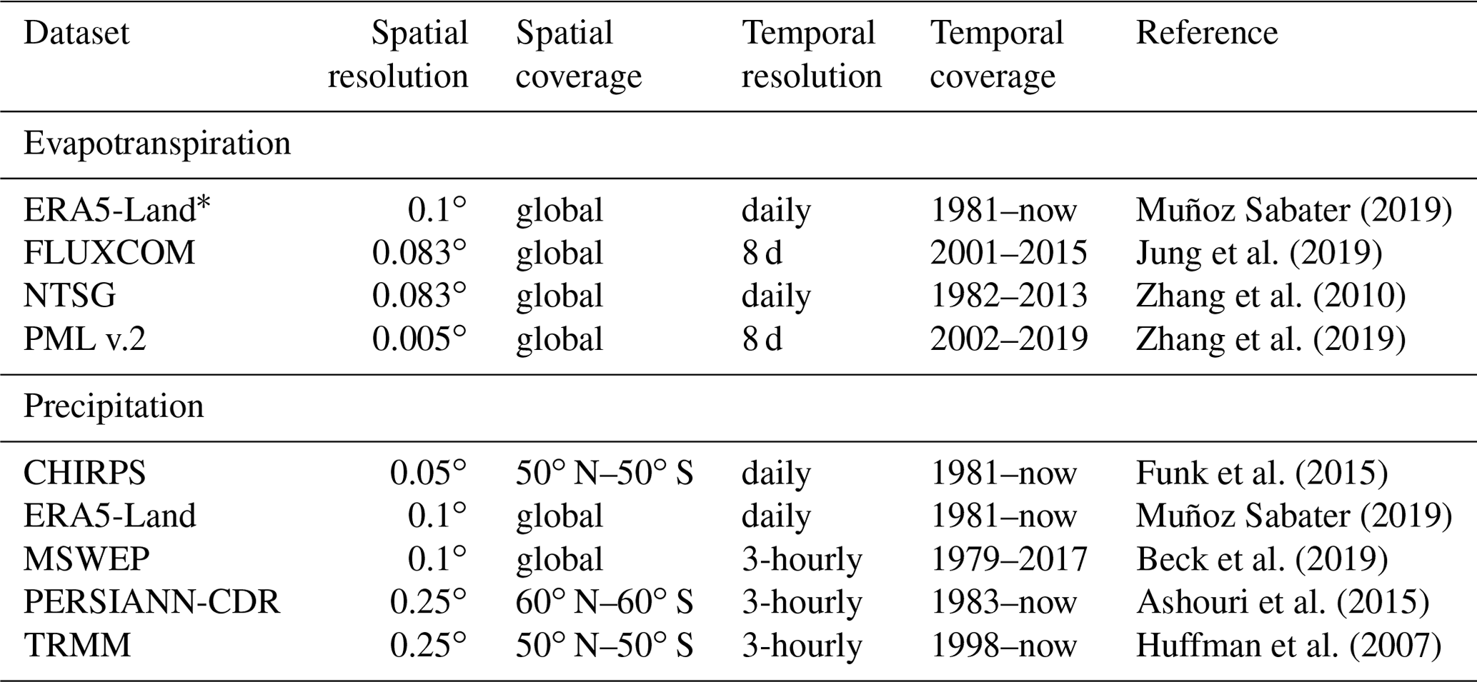
^* ERA5-Land ET is only used for validation of concept.

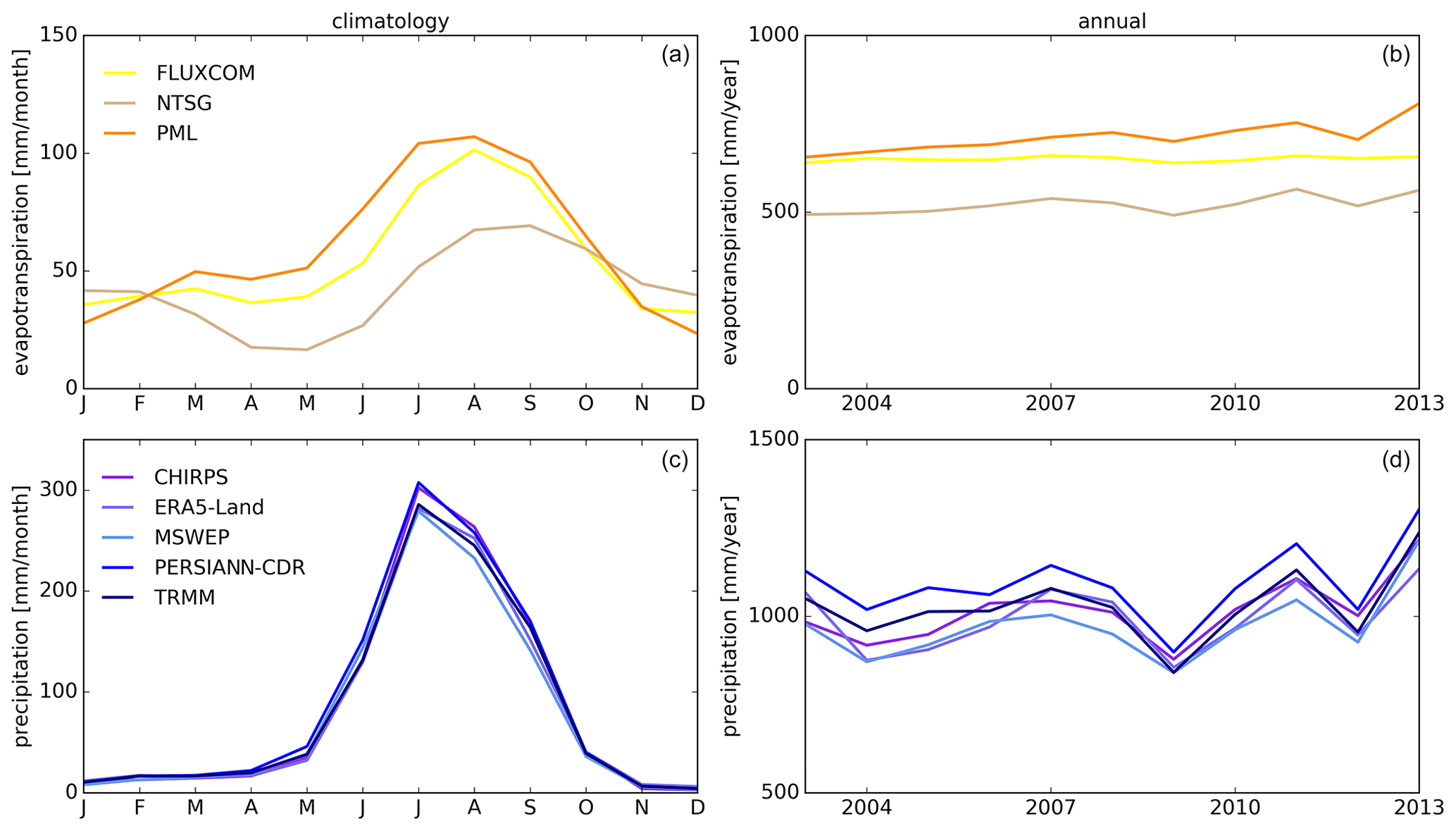
Figure 2 Regional climatologies and annual estimates of three evapotranspiration references (a, b) and five precipitation inputs (c, d) for the entire study area. Climatologies are based on available data from 2000 to 2020.

The five selected precipitation inputs are (1) the Climate Hazards Group InfraRed Precipitation with Stations (CHIRPS), (2) the fifth generation of the ECMWF reanalysis with enhanced resolution (ERA5-Land), (3) the Multi-Source Weighted-Ensemble Precipitation (MSWEP), (4) the Precipitation Estimation from Remotely Sensed Information using Artificial Neural Networks – Climate Data Record (PERSIANN-CDR), and (5) the Tropical Rainfall Measuring Mission (TRMM) Multi-satellite Precipitation Analysis (Table 1). CHIRPS uses reanalysis and satellite infrared data to estimate precipitation and gauge observations for correction (Funk et al., 2015). ERA5-Land is a high-spatial-resolution land component of the global ERA5 climate reanalysis system – a product driven by a large number of satellite and gauge data (Muñoz Sabater, 2019). MSWEP is a synthesis of different precipitation products that are merged using gauge observations (Beck et al., 2019). PERSIANN-CDR is a machine-learning product that uses satellite infrared data and gauge observations for bias correction (Ashouri et al., 2015). TRMM uses infrared and microwave satellite data to estimate precipitation and gauge observations for subsequent correction (Huffman et al., 2007). Precipitation products are very similar when comparing seasonal and annual variations and showed one distinct peak during the summer monsoon (Fig. 2c, d). However, relative differences of up to 40 % were found between the annual precipitation rates in the arid climate zone in the lower Indus Basin.

The three selected ET products are FLUXCOM, Numerical Terradynamic Simulation Group (NTSG), and Penman–Monteith–Leuning (Table 1). FLUXCOM is a machine-learning product that combines energy balance observations at flux towers with satellite data (Jung et al., 2019). NTSG is a satellite- and reanalysis-driven product that combines the Penman–Monteith and Priestley–Taylor models (Zhang et al., 2010). PML is a satellite- and reanalysis-driven product that is based on the Penman–Monteith and Leuning models (Zhang et al., 2019). All three products have the fact in common that they, to a large degree, utilize thermal and optical data from MODIS. The ET products were rather different with respect to their seasonal and annual variations but were generally characterized by two distinct peaks: the first in March and the second between July and September (Fig. 2a, b). The seasonal pattern is dominated by the summer monsoon and influenced by extensive irrigation during the dry period (December–April). The ET products were more similar during the dry period compared with the wet period, and relative differences were observed in annual ET across the basins in the humid (20 %) and arid (50 %) climate zones. Besides seasonal patterns, annual estimates suggest that ET and precipitation have increased since 2001 (Fig. 2b, d) which agrees with other studies (Jin and Wang, 2017; Katzenberger et al., 2021).

The selected products (Table 1) include different temporal and spatial resolutions, and all products have been preprocessed to the same spatiotemporal dimensions before modeling. The ET and precipitation products have been aggregated by summation to monthly and daily scales, respectively. Further, all ET products have been up- or downscaled to 5 km, and precipitation data were resampled to 10 km spatial resolution by bilinear interpolation.

3.4 Rainfed map

To calibrate the hydrological model against rainfed conditions (cropland that are not under irrigation), we created a map differentiating rainfed and irrigated cropland. The classification of cropland into rainfed and irrigated areas was based on MODIS land cover and normalized difference vegetation index (NDVI) products (MODIS MCD12Q1.v006 and MOD13Q1.v006). We found inspiration from Dari et al. (2021), who used results from a temporal stability analysis of satellite and modeled soil moisture in an unsupervised K-means analysis to detect and map irrigated areas. In our adopted approach, we used mean dry-period NDVI climatologies (i.e., 5 months, December–April) in a temporal stability analysis. More precisely, we used the standard deviation of the spatial anomalies and the temporal anomalies in a 2D unsupervised K-means classification to identify three clusters representing rainfed cropland, irrigated cropland, and mixed; more information about the temporal analysis components can be found in Dari et al. (2021). The assumption is that NDVI of rainfed cropland can be characterized by a high temporal stability and a low temporal anomaly in the 5 selected months, and vice versa for irrigated cropland. The classification was performed at the original MODIS resolution of 500 m and then upscaled to the model resolution, i.e., 5 km. A threshold of 95 % was used to identify primarily rainfed and irrigated pixels (to avoid a mixed rainfed and irrigated signal in the calibration); thus, a third class was added to represent pixels that were mixed. The classification was evaluated against the FAO Global Map of Irrigation Areas (GMIA) v5.0 dataset (Siebert et al., 2013) on global areas equipped for irrigation (Fig. 1) and showed overall consistency. During the wet period, cropland classified as “humid” according to the dryland classification by the Joint Research Center of the European Commission (Spinoni, 2015) was assumed to be rainfed cropland (Fig. 6e). The dry- and wet-period rainfed maps (Fig. 3) were used to correct the rainfed grids in the LAI climatologies, as described in Sect. 3.1.

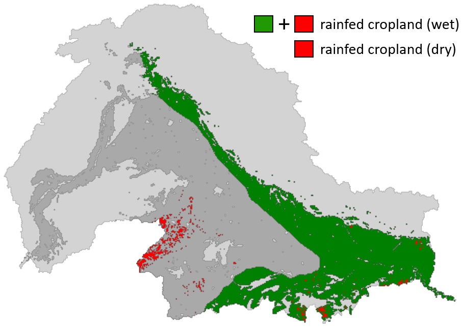
Figure 3 Map showing the classification of rainfed cropland applied in the evapotranspiration calibration during the dry (red) and wet (red and green) periods. The light gray signature delineates the Indus and Ganges basins, and the dark gray signature shows irrigated cropland in both dry and wet periods. Green indicates cropland that is only irrigated in the dry period.

3.5 Net irrigation estimation

Net irrigation is the amount of supplied irrigation that is lost through ET; thus, it does not account for return flows of irrigation water that drain to nearby rivers or recharge to groundwater. With that said, in complex irrigation systems like the Indus, studies indicate that the irrigation system is adapted to extensively reuse drainage water from irrigation (Simons et al., 2020). We assume that net irrigation can be quantified as the difference between an ET reference (ET references refer to different satellite products), obtained using methods such as remote sensing, and a hydrological model acting as a rainfed baseline (Koch et al., 2020). Net irrigation is quantified on a monthly timescale and at a 5 km spatial resolution for the 15 ensemble members, which are based on combinations of three ET and five precipitation products. We further assume that, by calibrating the 15 hydrological models against rainfed ET, we can simulate rainfed baselines for the entire model area that match the unique combination of ET and precipitation product. Our assumption is supported by the strong parameter regionalization schemes incorporated in mHM, which link model parameters to fully distributed catchment characteristics. This will yield physically meaningful parameter fields, which we believe are the foundation to make robust predictions of a rainfed baseline ET, including over irrigated areas. The magnitude of the ET products varies substantially (Fig. 2), and we hypothesize that calibration will enable the hydrological model to accommodate this, resulting in hydrological models with different magnitudes of rainfed ET to match the differences in the reference ET products. Uncertainties can be expressed as precision and accuracy. Precision investigates the ensemble dispersion, whereas accuracy is the closeness between estimates and observations. Thus, in the absence of observations, the accuracy of our net irrigation estimate cannot be quantified. Nevertheless, we believe that analyzing the precision of irrigation estimates is a valuable and novel contribution. We define net irrigation as the difference between ET as obtained from the reference products and the rainfed hydrological baseline model:

$$\begin{array}{}\text{(3)}& \mathrm{net}\mathrm{irrigation}={\mathrm{ET}}_{\mathrm{reference}}-{\mathrm{ET}}_{\mathrm{baseline}}.\end{array}$$

For rainfed areas, it is assumed that ET_reference is equal to the ET_baseline; thus, for irrigated areas, ET_reference is expected to exceed the ET_baseline, resulting in positive residuals (net irrigation). Negative residuals are a sign of an overestimation of the rainfed hydrological model and are treated as zero irrigation. If they occur, negative residuals can be related to uncertainties in the precipitation forcing, the ET product used as reference, or the hydrological baseline model itself.

3.6 Variance decomposition analysis

The model ensemble yielded 15 different net irrigation estimates, and we applied a variance decomposition analysis to investigate the sources of uncertainties in more detail. The uncertainty contribution from the two investigated sources, namely, the ET reference and precipitation on net irrigation, was analyzed following the approach of Déqué et al. (2007). This analysis quantifies the magnitude of net irrigation variance caused by the two uncertainty sources, thus ranking the influence of ET and precipitation. The procedure of the method is carried out in two steps. First, the variance contribution from both uncertainty sources and interactions between sources is calculated; thus, the total variance is the sum of all three variance contributions. Second, the variance term, as a percentage of the total variance, is calculated for each uncertainty source by summing the individual source variance and contributions from interactions and then dividing by the total variance. The sum of the two variance terms is more than the total variance, as the latter includes both the individual source variance and contributions from interactions between sources, but the magnitudes of the two variance terms indicate the individual role of each uncertainty source in the total variance (Déqué et al., 2007). The analysis was applied to monthly net irrigation estimates for each climate zone. The variance decomposition analysis has successfully been applied in a range of hydrological applications, for example, to study the uncertainty contributions of the climate model and hydrological model structure on climate change impact simulations (Karlsson et al., 2016). We acknowledge that this does not represent a complete uncertainty analysis, but we believe that the precipitation input and ET reference are the most important components for irrigation quantification.

4 Results and discussion

4.1 Baseline models

The Pareto fronts based on the 15 calibrations conducted (Fig. 4) show the trade-off between the two applied objective functions for rainfed ET, namely, MAE addressing the magnitude of ET and SPAEF addressing the spatial pattern performance. We tested different numbers of iterations and perturbation sizes before the calibration; based on our findings, we expect a higher number of iterations (more than 600) to only marginally improve the trade-off around the optimal solution but to primarily extend the tails of the Pareto fronts. In general, the range in the MAE of the Pareto fronts is larger than for SPAEF due to the assumption that model parameters can easily change the ET magnitude, but the simulated bias-insensitive spatial patterns are more realistic as a starting point. This is because the simulated spatial patterns are, to a large degree, linked to the spatial parameter fields which, again, are tied to fully distributed catchment characteristics, such as soil and vegetation variability. This will limit the range of SPAEF and rule out very poor pattern performance.

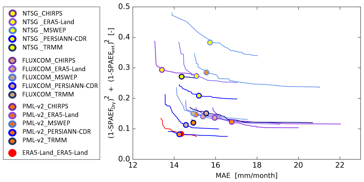
Figure 4 Calibration results for the 15 baseline models regarding the two defined objective functions: the MAE and SPAEF. The lines represent the Pareto fronts, containing the dominant solutions, and the points of the selected parametrizations with the optimal trade-off between objective functions. Point colors represent the three reference models and line colors represent the five precipitation inputs. The color scheme is consistent with the legends in Fig. 2.

Based on the Pareto fronts, the trade-off between the two applied objective functions can be studied, and we selected a single optimal parametrization for each of the 15 baseline models using the approach described in Sect. 3.2. The MAE of the 15 selected runs lies within a range of 13–17 mm per month, and the SPAEF varies between 0.44 and 0.76 during the dry period and between 0.60 and 0.85 during the wet period. The baseline models calibrated against the NTSG ET reference vary from the remaining models with an SPAEF that ranges between 0.44 and 0.63 during the dry period and between 0.70 and 0.74 during the wet period, thereby showing the poorest spatial pattern performance. This shortcoming relates to the homogeneous pattern in the satellite-based ET reference during the pre-monsoon period in April–May, which the baseline models cannot simulate. A list of calibration parameters and parameter bounds can be found in the Supplement (Table S1). The baseline model that was calibrated against the ERA5-Land reference and uses ERA5-Land precipitation is plotted as a 16th Pareto front in Fig. 4. For this calibration, the climate input and calibration target are obtained from the same modeling system and are, therefore, in good agreement. ERA5-Land does not directly incorporate irrigation and has, therefore, been used to validate the spatial parameter transfer between rainfed and irrigated areas. We calculated an MAE of 8.8 mm per month and an SPAEF of 0.83 for ERA5-Land over irrigated areas with parameters calibrated over rainfed conditions. We consider the high performance over irrigated areas to be a proof of concept that our calibration approach can reproduce a rainfed hydrological model. Rainfed ET bias time series and maps for ERA5-Land can be seen in Fig. S1 in the Supplement.

The ensemble ET baselines vary by about 200 mm yr⁻¹ – between 265 and 461 mm yr⁻¹ for the Indus Basin and between 473 and 674 mm yr⁻¹ for the Ganges Basin – which is the same total variability that is found across the ET references that the baselines were calibrated against. This implies that the ensemble baseline of rainfed ET is just as uncertain as the ET references; however, the aim is not to simulate the actual rainfed ET but to fine-tune each baseline hydrological model to their satellite-based ET reference and, thereby, enable a subtraction of rainfed ET from irrigated areas. Thus, a large range in ensemble baseline indicates that the calibration has served its purpose. Kushwaha et al. (2021) used an ensemble of hydrological models and applied the Budyko approach to estimate ET across the Indian subcontinental river basins; they found ET values in the Indus and Ganges basins in the range of 246–369 and 511–622 mm yr⁻¹, respectively.

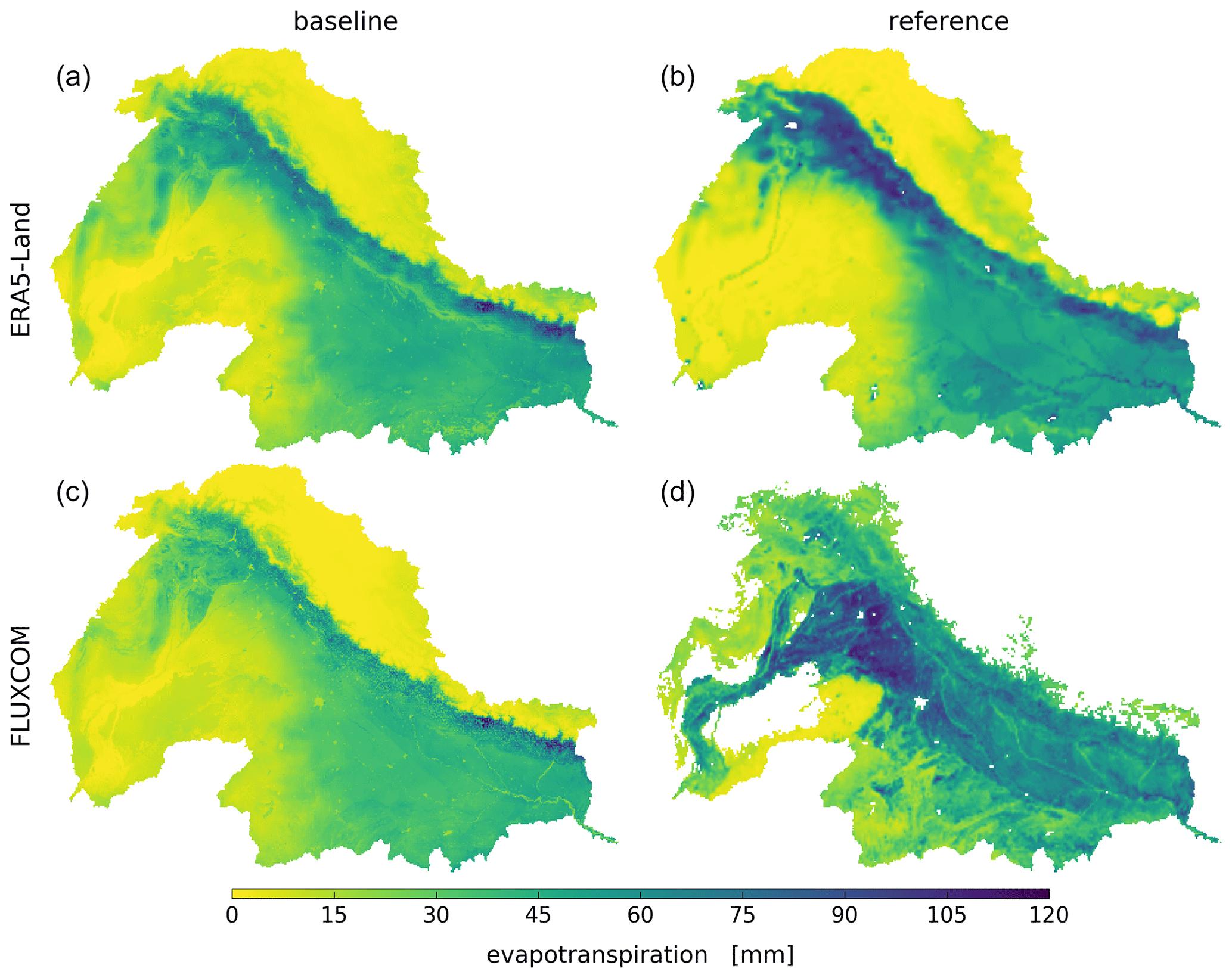
Figure 5 Average modeled baseline (a, c) and reference evapotranspiration (b, d) for February 2004. Both baseline models use ERA5-Land precipitation input.

The spatial patterns of the ET baselines are characterized by high ET along the Himalayan mountains and a regional east–west gradient matching the climatic zones (Fig. 5a, c). This emphasizes that the baselines simulate rainfed ET according to precipitation patterns (Fig. 5c, d). It becomes obvious that the ERA5-Land reference (Fig. 5b) does not consider the effect of irrigation on ET in the Indus and Ganges basins, and we found that only minor parts of the cropland are classified as irrigated in the ERA5 reanalysis model (ECMWF, 2018). As irrigation does not affect ERA5-Land, the spatial patterns of the ERA5-Land baseline (simulated by mHM) and ERA5-Land ET reference (Fig. 5a, b) are expected to also match for irrigated areas. We calculated the SPAEF between the ERA5-Land baseline and reference ET for rainfed and irrigated cropland and found the SPAEF for rainfed and irrigated cropland to be 0.79 and 0.88, respectively, which means that the baseline and reference ET match well in both rainfed and irrigated areas. We found that the ERA5-Land baseline was able to reproduce the natural precipitation-induced ET patterns in the irrigated areas but showed minor elevated ET in the desert due to model uncertainty.

This underpins the validity of the method, i.e., that a hydrological model can be calibrated to reproduce rainfed ET originating from an alternative reference. By comparing the FLUXCOM baseline and reference (Fig. 5c, d), the ET baseline magnitude is similar to the ET reference for rainfed areas and the spatial pattern resembles precipitation patterns. Thus, the hydrological model can simulate a realistic rainfed ET baseline. As ERA5-Land does not account for irrigation, the product is not used in the ensemble estimates described in Sect. 4.2.

4.2 Net irrigation ensemble estimates and precision

The analysis is based on an ensemble of 15 independent net irrigation estimates (hereafter referred to as ensemble estimates). The main finding of the analysis is that the standard deviation of the ensemble estimates is low in most of the study area (Fig. 6b). Although the ensemble baselines, i.e., the simulated rainfed ET of the 15 models, differ by about 91.5 mm yr⁻¹, the net irrigation precision is 44.7 mm yr⁻¹ for the entire region. This indicates that the magnitude of ET variation induced by irrigation within each ET reference yields net irrigation estimates of comparable magnitudes.

The ensemble estimates of the dry period (Fig. 6a) show high net irrigation across the Indo-Gangetic Plain. As expected, net irrigation is largest in the northern Punjab region (Sharma et al., 2010), and a decrease from west to east following the transition from arid to humid climatic zones (Fig. 6e) can be observed. Dry-period ensemble estimate precision is evenly distributed across all four climate zones (Fig. 6b), illustrating the importance of calibration to obtain comparable net irrigation magnitudes from references with different ET magnitudes. The wet-period ensemble estimate (Fig. 6c) shows high net irrigation in the arid zone, which we did not expect. The precision is highly correlated in space during the wet period, expressed by a cluster of low precision, i.e., high standard deviation, in the arid zone (Fig. 6d). Based on further analysis, we relate this effect to the apparent overestimation of FLUXCOM and PML ET references. During the wet season, these products show very limited spatial variation in ET within the entire arid zone and are, thus, characterized by a very high, uniform ET rate. Contrarily, NTSG and the hydrological models show distinct spatial variations within the arid zone that relate to variability in vegetation and soil texture. Therefore, the ensemble precision is low in the arid zone.

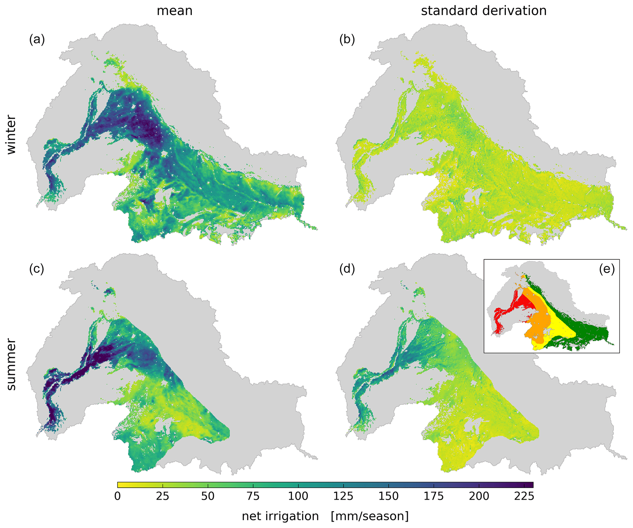
Figure 6 Mean ensemble net irrigation estimates (a, c) and ensemble standard deviation (b, d) for the dry period (a, b) and wet period (c, d). (e) Dryland classification by the Joint Research Center of the European Commission (Spinoni, 2015), where red denotes arid, orange denotes semiarid, yellow denotes dry, and green denotes humid; climate data can be seen in Fig. 1.

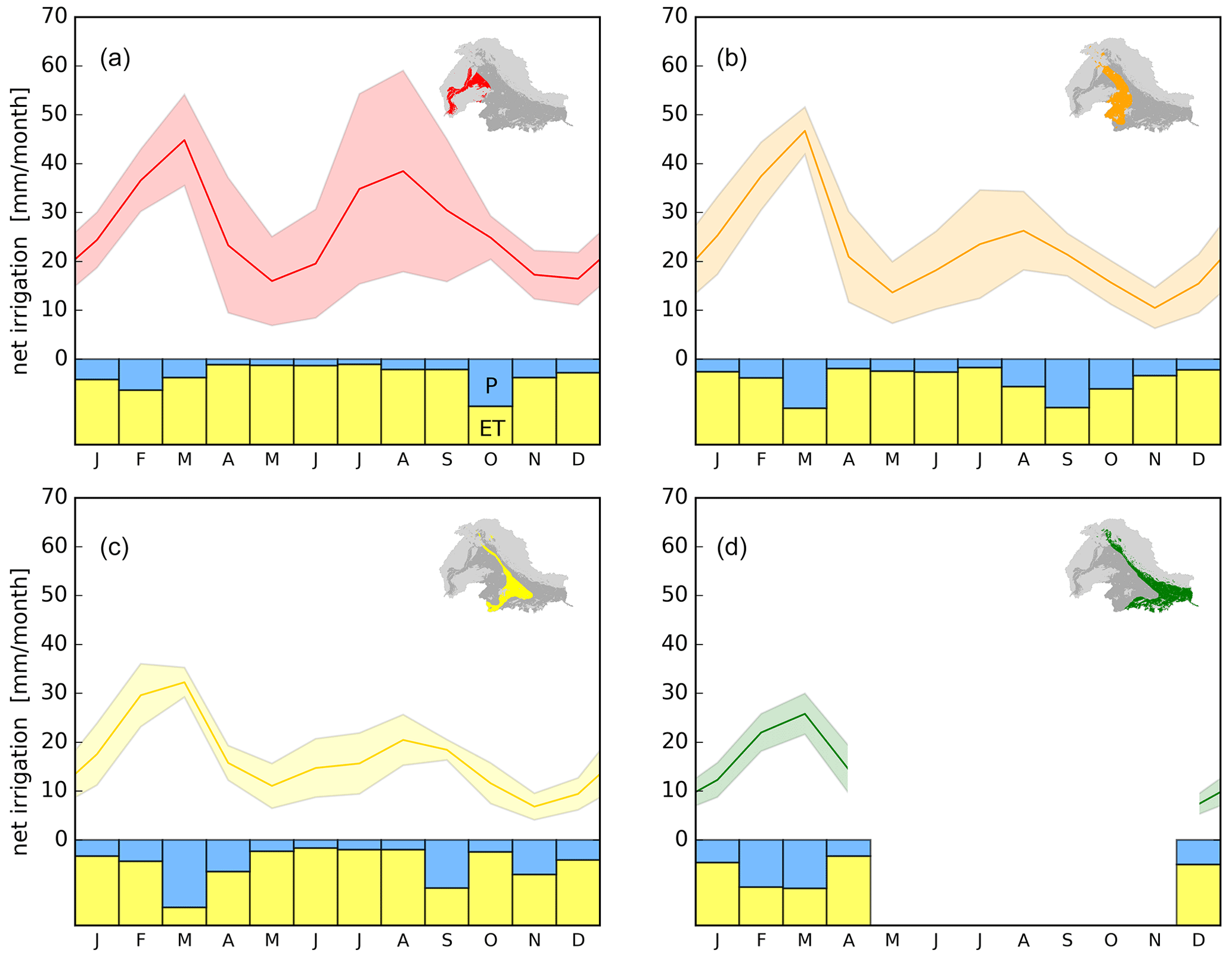
Figure 7 Temporal ensemble net irrigation estimates and precision for each climate zone: (a) arid, (b) semiarid, (c) dry, and (d) humid. The solid line indicates the mean monthly net irrigation, whereas the shaded envelope indicates the precision as ±1 SD (standard deviation). The lower bar charts illustrate results from the variance decomposition analysis and show the degree to which evapotranspiration (ET, yellow) and precipitation uncertainty (P, blue) explain the ensemble variance.

Table 2 Overview of ensemble net irrigation estimates and precision for the Indus and Ganges basins separately and aggregated as a region. The wet-period net irrigation and precision are calculated according to dry-period irrigated cropland.

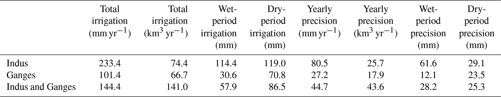
The temporal variation in the ensemble estimates and their precision (Fig. 7) show that net irrigation estimates peak during February–March in the entire region and that precision is well defined at a monthly scale, except in the arid zone during the wet period (Fig. 7a). The mean ensemble estimate and precision in the Indus Basin are estimated to be 233.4±80.5 mm yr⁻¹ (74.4±25.7 km³ yr⁻¹) and the mean ensemble estimate and precision in the Ganges Basin are estimated to be 101.4±27.2 mm yr⁻¹ (66.7±17.9 km³ yr⁻¹) (Table 2). This highlights the higher intensity of irrigation in the Indus Basin, as the total irrigation water use is about the same as the Ganges Basin despite the substantially smaller cropland area (Indus: 796.8×10⁶ ha; Ganges: 1643.4×10⁶ ha). Aggregated seasonal ensemble estimates indicate that net irrigation in the Indus Basin is evenly split between the dry and wet periods (51 % and 49 %, respectively), whereas 70 % of net irrigation in the Ganges Basin occurs during the dry period. The mean ensemble estimate and precision aggregated for both the Indus and Ganges basins are estimated to be 144.4±44.7 mm yr⁻¹ (141.0±43.6 km³ yr⁻¹), resulting in a precision of 31 % for the total irrigated water use. By comparing basin and regional ensemble estimates, the regional estimate is influenced by the lower precision in the Indus Basin during the wet period. Therefore, we want to highlight a precision of 18 % (25.3 mm per season) in both basins during the dry period (Table 2).

The mean monthly standard deviation was found to depend on the climatic zones and decreased from 8 to 4 mm per month during the dry period and from 12 to 5 mm per month during the wet period as the aridity index increased, i.e., going from arid to humid climate. This overall increase in precision across the four climate zones (Fig. 7a–d) coincides with a decrease in the ET reference uncertainty. Estimating ET can be very difficult under extreme climatic conditions, such as those experienced in arid zones, and is strongly dependent on the modeling approach (Jung et al., 2019; Zhang et al., 2019). This is also evident in our initial analysis of 10 different reference models. A comparison of the seasonal coefficients of variation shows that the standard deviation is 37 % of the mean net irrigation during the wet period and 27 % during the dry period, which is consistent in both basins. Lower precision during the wet period has been reported for irrigation quantifications using alternative soil-moisture-based approaches (Jalilvand et al., 2019; Zohaib and Choi, 2020) and results from less irrigation being used to supplement precipitation during the wet period, whereas irrigation largely replaces precipitation during the dry period. Therefore, it can be difficult to isolate the net irrigation signal from ET affected primarily by precipitation during the wet period.

The uncertainty of the rainfed ensemble baselines is evaluated based on ET residuals over rainfed cropland that have a mean error of 32.5 mm yr⁻¹, corresponding to a 5.2 % error. This low bias implies that the baseline models were able to reliably simulate rainfed ET that matches the ET references and can be understood as a measure of accuracy under the assumption that the simulation bias over rainfed cropland can be transferred to irrigated cropland. For irrigation quantification for the North China Plain, Koch et al. (2020) found that the accuracy was highest during the monsoon season due to energy-limiting conditions. We found the accuracy to be equally high in both wet and dry periods. We assume that this is due to the skewed weight on wet-period rainfed cropland during the calibration, as this area is much larger than dry-period rainfed cropland (Fig. 3). The precision of the ensemble estimates (44.7 mm yr⁻¹) can be attributed to ET and precipitation uncertainties, whereas the accuracy (32.5 mm yr⁻¹) can be attributed to uncertainties originating from the hydrological model, ET references, and precipitation uncertainties. This implies that the precision and accuracy are not independent in our case and that the total variance is not simply the sum of the two.

The comparison of irrigation estimates can be challenging, as notions might cover different aspects like irrigation water withdrawal, irrigation water requirement, or net irrigation as the ET loss to the atmosphere. Simons et al. (2020) used remote-sensing data and the Budyko framework to quantify irrigation water use and found consumed fractions to be 0.71–0.93 in the Indus Basin irrigation system of Pakistan due to the substantial reuse of unconsumed water. Our estimates could therefore potentially underestimate irrigation water use by 10 %–30 % within Pakistan. The consumed fractions were based on actual ET estimates from the operational Simplified Surface Energy Balance (SSEBop) v4 model that we had to reject due to a significantly higher yearly actual ET. Our pre-analysis of SSEBop could potentially explain why our irrigation estimates are several hundred millimeters lower than the 707 mm yr⁻¹. Overestimation of the actual ET and potential ET within the Budyko framework could yield higher irrigation water use and underestimate the consumed fractions. However, we acknowledge that our framework cannot account for the total irrigated water use. Karimi et al. (2013) used a water accounting framework (WA+) to track water within the Indus Basin for the year 2007 and found ET from utilized water flows to amount to 157 km³, which is higher than our estimate of 74.4±25.7 km³ yr⁻¹. In Karimi et al. (2013) the yearly actual ET is also several hundreds of millimeters higher than the three ET references used in our study. Water statistics from the AQUASTAT database estimated a yearly irrigation water requirement in Pakistan (126 km³ yr⁻¹) and India (370 km³ yr⁻¹). The estimates are based on climatic conditions and crop physiological processes and encompass all water to meet crop water requirements, water for flooding of paddy fields, water for land preparation, etc. (Frenken and Gillet, 2012). Based on the assumption that the yearly irrigation water requirement estimated by AQUASTAT is true, our net irrigation estimates suggest that about 31 % of the total irrigation water requirement for the entire Indian subcontinent is lost through ET in the Indus and Ganges basins.

We found the difference, due to irrigation in cropland, between the baseline and reference ET to be 55 % and 14 % in the Indus and Ganges basins, respectively. However, a 55 % increase might be an overestimation that arises from the FLUXCOM and PML references. If only considering the NTSG baseline and reference ET, the change in the Indus Basin is found to be 37 %, which seems to be more appropriate. Shah et al. (2019b) used a soil moisture deficit approach and estimated a percent change in ET between a natural and irrigated scenario modeled with the Variable Infiltration Capacity model. They found an annual ET increase of 47 % and 12 % in the respective Indus and Ganges basins from 1951 to 2012 because of irrigation activities. The mismatch compared with our reported figures could result from their irrigation timing being off, thereby allowing irrigation to occur in between harvest and sowing when the fields are fallow; however, overall, there is a good match of results. Shah et al. (2019a) incorporated reservoirs and irrigation water demand into the model framework from Shah et al. (2019b) and found that ET increased by about 16.1 % and 15.7 % in the Indus and Ganges basins, respectively. Our results compare well with this estimate for the Ganges Basin. In both studies (Shah et al., 2019a, b), the natural model seems to be calibrated against data that could potentially be influenced by irrigation, like irrigation water demand (only Shah et al., 2019a) and streamflow, which could underestimate ET in a managed scenario.

4.3 Influence on ensemble precision

The main finding of our variance decomposition analysis is a strong ET control on ensemble estimate variance. ET accounts for 73 % of the ensemble estimate precision across the basins, and the influence of precipitation is observed to increase in more humid climate zones (blue and yellow bars in Fig. 7). However, the contribution of precipitation becomes more prominent in the monsoon season from July to September and around March (Fig. 7) and, thus, tends to follow the precipitation climatology (Fig. 2c).

The ET reference and any related uncertainties affect the baseline ET estimates through the calibration, and the net irrigation estimation (as the baseline ET) is subtracted from the reference ET. On the other hand, precipitation uncertainty only affects the baseline ET models. Therefore, the reference ET directly affects the net irrigation estimates, whereas precipitation uncertainty acts indirectly as it is propagated through the hydrological model to impact the baseline ET. Furthermore, precipitation uncertainty between irrigated and rainfed cropland is likely similar, whereas uncertainty between irrigated and rainfed ET may vary in the reference ET products.

Thus, it is difficult to conclude whether the influence of precipitation increases because of the uncertainty or increases because the ET uncertainty decreases. The fact that the influence of precipitation tends to follow the seasonal variation in precipitation emphasizes that ET residuals are more difficult to extract during high precipitation (Koch et al., 2020). In the arid zone, the influence of ET is higher during the wet period, which is due to the high ET uncertainty and potential errors in FLUXCOM and PML products. The ET uncertainty seems to overrule the high precipitation uncertainty in the arid zone, even though ERA5-Land and MSWEP precipitation inputs are about 40 % lower than the other precipitation inputs.

5 Conclusion

This study focuses on an ET-based approach to estimate irrigation water use for the Indus and Ganges basins, a global hotspot of unsustainable irrigation practices. We investigated the influence of different ET reference models and precipitation inputs on the precision of irrigation estimates by analyzing an ensemble of 15 net irrigation estimates. We showed that isolating the irrigation component through ET residuals of rainfed ET baselines and reference ET models yields high-precision estimates of net irrigation.

The main findings of this work are as follows:

• We estimated net irrigation of the Indus and Ganges basins to be 144.4±44.7 mm yr⁻¹, of which about half of the irrigation takes place in the Indus Basin, despite the fact that the Indus Basin accounts for only 35 % of the irrigated cropland areas.

• We found that, even though ET varied by 91.5 mm yr⁻¹ between reference ET products, the precision of net irrigation was just 25.3 mm per season during the dry period.

• We found that net irrigation precision increased as reference ET uncertainty decreased, which was related to the climatic conditions of the area.

• We found that ET accounted for 73 % of net irrigation variance and that the influence of precipitation uncertainty was highest during the monsoon season from July to September.

We emphasize the strength of model calibration to compensate for ET biases to create robust net irrigation estimates. As large differences in seasonal and annual rainfed ET may be evident between reference models, the magnitude of ET variation induced by irrigation within each ET reference yields net irrigation estimates of comparable magnitudes. Therefore, it is essential to calibrate and fine-tune each baseline model to a reference rainfed baseline to extract net irrigation.