Producing reliable hydrologic scenarios from raw climate model outputs without resorting to meteorological observations

A simplified hydroclimatic modelling workflow is proposed to quantify the impact of climate change on water discharge without resorting to meteorological observations. This alternative approach is designed by combining asynchronous hydroclimatic modelling and quantile perturbation applied to streamflow observations. Calibration is run by forcing hydrologic models with raw climate model outputs using an objective function that excludes the day-to-day temporal correlation between simulated and observed hydrographs. The resulting hydrologic scenarios provide useful and reliable information considering that they (1) preserve trends and physical consistency between simulated climate variables, (2) are implemented from a modelling cascade despite observation scarcity, and (3) support the participation of end-users in producing and interpreting climate change impacts on water resources. The proposed modelling workflow is implemented over four sub-catchments of the Chaudière River, Canada, using nine North American Coordinated Regional Climate Downscaling Experiment (NA-CORDEX) simulations and a pool of lumped conceptual hydrologic models. Results confirm that the proposed workflow produces equivalent projections of the seasonal mean flows in comparison to a conventional hydroclimatic modelling approach. They also highlight the sensibility of the proposed workflow to strong biases affecting raw climate model outputs, frequently causing outlying projections of the hydrologic regime. Inappropriate forcing climate simulations were however successfully identified (and excluded) using the performance of the simulated hydrologic response as a ranking criterion. Results finally suggest that further works should be conducted to confirm the reliability of the proposed workflow to assess the impact of climate change on high- and low-flow events.

1 Introduction

Assessments of climate change impacts are commonly oriented in a top-down perspective favouring the implementation of a modelling cascade from greenhouse gas concentrations to hydrologic (impact) models (e.g. Poulin et al., 2011; Seiller and Anctil, 2014; Seo et al., 2016). Since climate models are affected by uncertainties that limit their ability to simulate atmospheric processes at the local scale, statistical post-processing is typically applied to bias-correct their (raw) outputs to improve agreement with in situ observations. The product of a post-processed climate simulation is often termed the climate scenario: a plausible trajectory that originally shares the statistical properties of the local (reference) recent past and evolves along physically based long-term trends (Huard et al., 2014). The resulting climate scenarios are subsequently translated into simulated streamflow series using calibrated hydrologic models.

Usage of post-processed climate model outputs is criticized for three main reasons (e.g. Alfieri et al., 2015b; Chen et al., 2018; Lee et al., 2018): (1) it disrupts the physical consistency between simulated climate variables, (2) it affects the trend in climate change signals imbedded within raw climate simulations, and (3) it requires abundant good-quality meteorological observations, which are unavailable for many regions of the world, including some less common meteorological fields such as wind speed, relative humidity, and radiation (Ricard et al., 2020). More marginal critics raise the fact that statistical post-processing hides raw climate model output biases from end-users (Ehret et al., 2012), potentially blurring the confidence attributed to resulting impact scenarios and misleading adaptation to climate change. Even if these limitations are generally acknowledged, statistical post-processing is often considered mandatory for climate change impact assessment studies on water resources. Trend-preserving and multi-variate approaches (e.g. Cannon et al., 2018; Ahn and Kim, 2019; Nguyen et al., 2020) have been specifically developed in order to limit the above-mentioned post-processing drawbacks. However, these approaches involve a fairly high level of complexity and, consequently, require specific expertise in post-processing technologies.

In the scientific literature, raw climate model outputs are mostly used as benchmarks to assess the performance issued by post-processed climate model outputs (e.g. Teng et al., 2015; Ficklin et al., 2016; Charles et al., 2020). The use of raw climate model outputs as hydrologic scenarios is a marginal practice, mostly because resulting streamflow simulations are correspondingly affected by biases (e.g. Muerth et al., 2013) and by the lack of synchronicity between the simulated climate and the observed hydrologic (river discharge) time series. Such implementation is mostly justified when focusing on relative changes to reference conditions (Alfieri et al., 2015a, b) or under the assumption that climate model output biases are sufficiently small to be compensated for by the calibration of the hydrologic model (Chen et al., 2013). This is also justified when extreme events are analysed considering the uncertainty introduced by the short sampling of observation chronicles (Meresa and Romanowicz, 2017). Advocating the benefit of preserving the dependence between simulated climate variables, Chen et al. (2021) recently constructed hydrologic scenarios from raw climate model outputs by applying the daily-translation bias-correction method (Mpelasoka and Chiew, 2009) to streamflow simulations instead of climate simulations. The authors demonstrated that the approach reduces hydrologic biases comparably to a conventional one for which climate simulations are corrected beforehand. They finally highlighted that, regardless of the modelling approach, climate simulations issue poor hydrologic responses due to the non-stationarity of the climate biases and abrupt seasonal fluctuations affecting correction factors.

Most climate change studies resort to a modelling cascade for which the hydrologic model is calibrated independently of the climate model outputs, using observations as meteorological forcings (e.g. Poulin et al., 2011; Seiller and Anctil, 2014; Seo et al., 2016). This is questionable since calibration then compensates errors from meteorological observations (e.g. solid precipitation undercatch or spatial interpolation of in situ observations) but not to those from climate models outputs. It consequently influences the identification of hydrologic model parameters, as well as the representation of hydrologic processes simulated at the catchment scale. The resulting effect on the hydrologic scenarios and projected changes in the water regime components remains mostly misunderstood. Few studies conducted calibration by forcing hydrologic models directly with raw climate model outputs. Chen et al. (2017) quantified the hydrological impacts of climate change over North America, calibrating a lumped conceptual hydrologic model with raw regional climate model (RCM) outputs over a recent past period. Ricard et al. (2019) proposed an alternative configuration of the hydroclimatic modelling chain and tested five objective functions that exclude the temporal synchronicity of hydrologic events, such as the correspondence between observed and simulated targeted quantiles, distribution moments, mean flows, or annual cycles. They concluded that forcing a physically based hydrologic model with regional climate simulations according to asynchronous modelling principles can improve the simulated hydrologic response over the historical period. Ricard et al. (2020) implemented statistical post-processing of raw climate model outputs within the asynchronous modelling framework by calibrating quantile mapping transfer functions together with the parameters of the hydrologic model. They integrated relative humidity, solar radiation and wind speed, for which observations are scarce or unavailable, to a modelling chain and confirmed the improvement of the simulated hydrologic response in comparison to a conventional framework using reanalyses as a description of the reference climate.

This study proposes a straightforward hydroclimatic modelling workflow enabling the production of streamflow projections without post-processing climate model outputs and without using meteorological observations. The procedure is inline with the modelling frameworks experimented by Ricard et al. (2020) and Chen et al. (2021). In essence, the workflow translates raw climate model outputs into a corresponding simulated hydrologic response using an asynchronous framework that encrypts simulated hydrologic changes by defining change factors for each streamflow quantiles. When relative trends are required, a qualitative climate change impact assessment can be conducted by analysing the distributions of change factors. When hydrologic time series are required, the change factors can be applied on the available streamflow observations. This approach, referred to as quantile perturbation, has been previously applied to climate model outputs (e.g. Sunyer et al., 2015; Willems and Vrac, 2011) but not, to our knowledge, using streamflow simulations resulting from a hydroclimatic modelling cascade. The key advantage of the proposed approach is that meteorological observations are not required, nor for post-processing climate model outputs, nor for calibrating the hydrologic model. It is thus easy to implement compared to the conventional modelling cascades, which are typically affected by much heavier requirements in terms of data, modelling processes, and computing capacity. The workflow also preserves trends and consistency between simulated climate variables and allows for a bottom-up assessment of raw climate model outputs from the perspective of the impact modeller and end-user expertise. The study also aims to assess and discuss its reliability by comparison to a conventional hydroclimatic modelling, involving post-processing of raw climate model outputs and calibration of hydrologic models using meteorological observations. Section 2 presents the watershed of interest of the data used in the study. Section 3 explains the methodological specificities of the proposed workflow and describes its implementation using raw North American Coordinated Regional Climate Downscaling Experiment (NA-CORDEX) simulations over a mid-scale catchment located in southern Quebec, Canada, and a pool of lump conceptual hydrologic models. Section 4 displays results, while Sect. 5 discusses the strengths and weaknesses of the proposed modelling workflow.

2 Watershed of interest and data

The study is conducted over four sub-catchments of the Chaudière River (Fig. 1), a 185 km river that takes its source in Lake Mégantic (altitude 395 m) and flows northward into the St. Lawrence River, near Québec City. The 6694 km² catchment is located in the southern part of the province of Quebec, Canada, bordering the United States at its meridional delineation. It is shaped by a moderate topography (the highest peak is 1100 m) mostly corresponding to the Appalachian geological formation upstream and the St. Lawrence Lowlands downstream. The river slope is steep (∼ 2.5 m km⁻¹) upstream of the town of Saint-Georges (site 4, Fig. 1) and abruptly gentles to ∼ 0.5 m km⁻¹ down to Saint-Lambert (site 2). The catchment is mostly covered by forest (∼ 70  %), but agricultural land uses are nonetheless substantial (∼ 23  %), mostly in the lower portion of the catchment. The Chaudière River frequently floods from Saint-Georges down to Saint-Lambert and is also prone to ice jams, mostly around Beauceville (roughly 10 km downstream of Saint-Georges).

The climate is humid continental (Dfb according to the Köppen classification). The mean annual temperature shows marked seasonal fluctuations (see Fig. 3), falling below freezing roughly from November to March. Total annual precipitation is around 1000 mm, depicting no seasonal fluctuations except for a mild intensification from August to November. The corresponding hydrologic regime can be categorized as nivopluvial, corresponding to an alternation of two dominant flood periods. Driven by snowmelt and rainfall, the main flood period takes place from March to April, while the secondary in autumn is driven by an increase in precipitation. These two flood-prone periods are punctuated by two low-flow periods. The flow regime is mostly free from the influence of dam operation, except for short river reaches downstream of Mégantic and Sartigan dams (located at Mégantic Lake and upstream from Saint-Georges, respectively).

Nine NA-CORDEX simulations (Mearns et al., 2017; Table 1) are used to construct the hydrologic scenarios. They consist of 50 km RCM simulations that are driven by four global climate models (GCMs) forced by the RCP8.5 greenhouse gas (GHG) concentrations. One to four grid cells cover the study area, depending on the RCM. Daily minimum and maximum 2 m air temperature and daily precipitation were archived over a reference historical period from 1970 to 1999 and a future period from 2040 to 2069. Since no statistical post-processing is applied in the proposed modelling workflow, RCM simulations are preferred to GCM simulations to minimize the scale mismatch between the climate models and the in situ observations. RCP8.5 is preferred over RCP4.5 for its more pronounced climate change signal and because more NA-CORDEX simulations are then available. Since the studied catchment features a topography of moderate complexity and a medium area of 6694 km², a 50 km horizontal resolution was considered sufficient over the finer but smaller ensemble of 25 km simulations. Other climate change impact studies have relied on a comparable number of RCM simulations (e.g. Alfieri et al., 2015a, b; Laux et al., 2021).

Daily discharge observations are collected from the Quebec hydrometric network (MELCC, 2021). Stations located at the outlets of the four sub-catchments of the Chaudière River are described in Table 2. The four sub-catchments encompass 87  % of the area of the Chaudière River catchment, and only the very downstream part is ungauged. Hydrometric stations 023402 (site 2) and 023429 (site 4) are located on the main river, while stations 023401 (site 1) and 023422 (site 3) are located on the Beaurivage and Famine rivers, two important effluents (709 and 691 km², respectively). Streamflow observational record lengths are fairly long according to North American standards. Standards 023401 and 023402 have been in operation since the early 20th century and standards 023422 and 023429 from 1964 and 1969, respectively. The gridded observation datasets (daily air temperature and precipitation) are derived from kriging in situ data at 0.1^∘ resolution from 1970 to 2018 (Bergeron, 2015). For the study, we extracted the observed time series from 1970 to 1999.

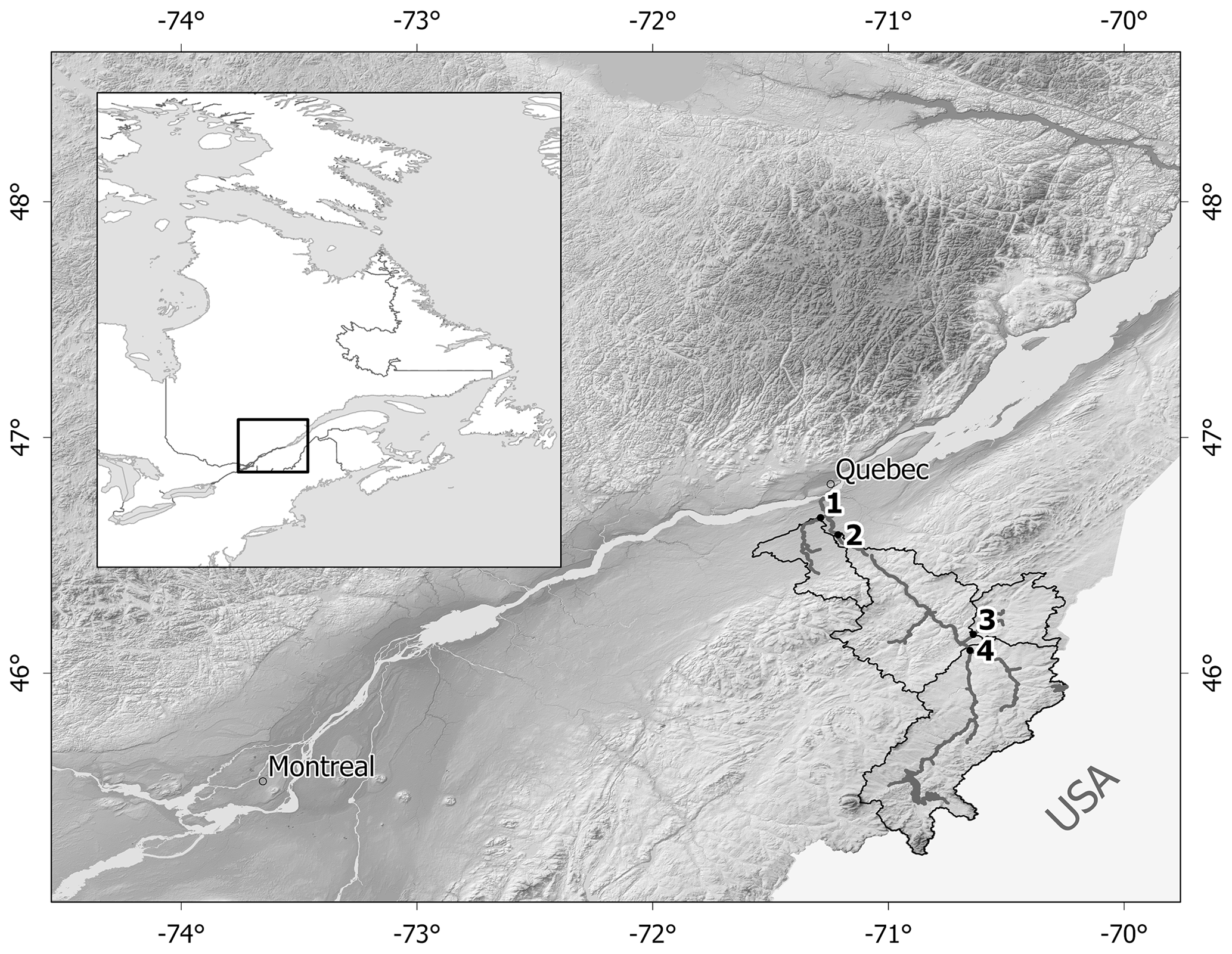
Figure 1 Locations of the Chaudière River and sub-catchments described in Table 2. Sites 1 to 4 correspond to the locations of hydrometric stations.

Table 1 Description of North American CORDEX simulations.

Table 2 Description of the Chaudière River sub-catchments.

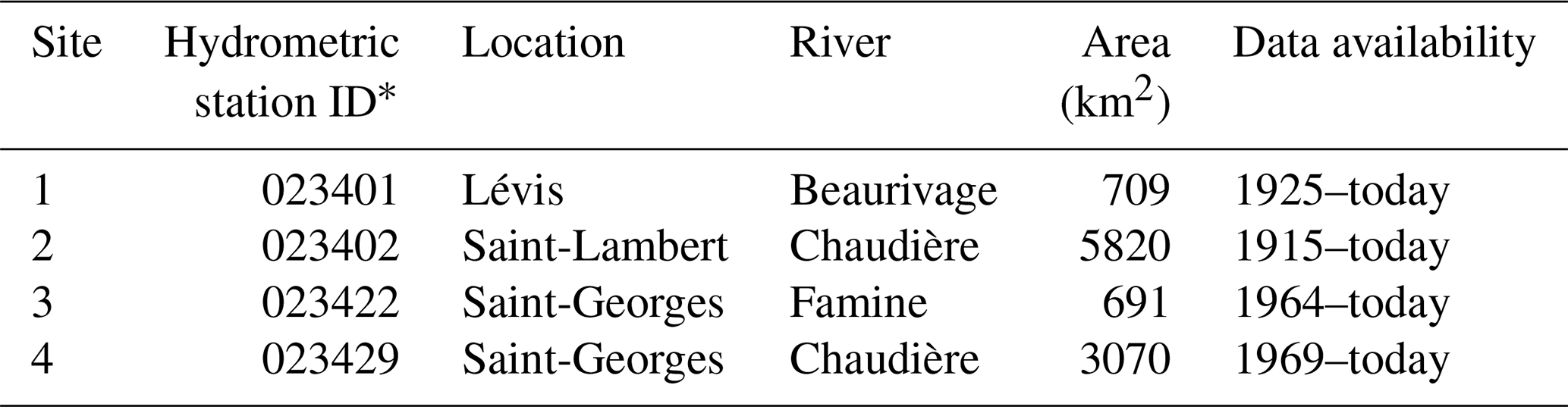
^* Notification attributed by the Quebec hydrometric network (MELCC, 2021).

3 Methods

3.1 The proposed asynchronous modelling workflow

The asynchronous modelling framework was previously explored by Ricard et al. (2019, 2020), mainly focusing on testing calibration metrics and implementing a more complex description of hydrological processes. Asynchronous modelling is analogous to a signature-based modelling in the way it aims to identify parametric solutions by optimizing the statistical properties of the simulated hydrograph, capturing the broad hydrologic behaviour of a catchment instead of the precise sequence of hydrometeorological events observed at the outlet. The purpose of asynchronous modelling is however different from signature-based modelling since it proposes constructing hydrologic scenarios according to a specific reconfiguration of the conventional hydroclimatic modelling chain, circumventing the requirement for meteorological observations typically used for post-processing raw climate model outputs and calibrating the hydrologic model.

The proposed asynchronous modelling workflow (Fig. 2) follows three main steps: (1) translating raw climate model outputs into corresponding hydrologic responses using asynchronous modelling, (2) computing change factors derived from a reference and a future simulated hydrologic response, and (3) constructing hydrologic scenarios by applying correction factors to the available streamflow observations. Asynchronous hydroclimatic modelling (Ricard et al., 2020) refers to an alternative configuration of the hydroclimatic modelling chain for which the calibration is performed on climate model outputs (over a recent past reference period) and not on meteorological observations. Since climate models cannot reproduce the observed sequence of meteorological events, we expect correlation-based calibration metrics (such as Nash–Sutcliffe efficiency – NSE – and Kling–Gupta efficiency – KGE) to mislead the identification of calibrated parameters within the asynchronous framework. The parameters of hydrologic models are thus optimized according to an objective function that purposely excludes the day-to-day temporal correlation (Ricard et al., 2019).

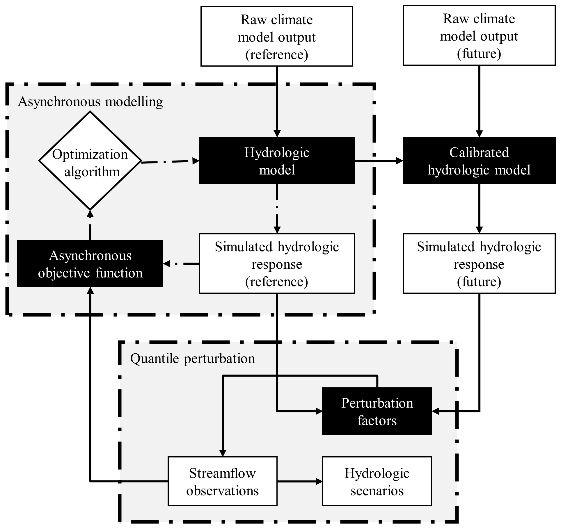
Figure 2 The proposed asynchronous modelling workflow. In comparison to a conventional hydroclimatic modelling approach, the production of hydrologic scenarios does not require meteorological observations, not for post-processing raw climate modelling nor for calibrating the hydrologic model. A detailed description of the conventional modelling approach is provided by Ricard et al. (2020).

The calibration loop trains the hydrologic model in reproducing the statistical properties of the streamflow regime, such as the form of its cumulative distribution, quantiles, or moments, without taking into account the temporal match between them. We propose here a normalized score inspired by the continuous-ranked probability score (CRPS) (Matheson and Winkler, 1976), where the distribution of simulated streamflow is compared against the distribution of observations – the CRPS is commonly used to assess ensemble prediction systems. More specifically, the proposed score is defined such that

$$\begin{array}{}\text{(1)}& \mathrm{nCRPS}\left(F,x_{\mathrm{obs}}\right)={\int }_{-\mathrm{\infty }}^{\mathrm{\infty }}{\left(F\left(\stackrel{\mathrm{̃}}{x}\right)-F\left({\stackrel{\mathrm{̃}}{x}}_{\mathrm{obs}}\right)\right)}^{\mathrm{2}}\mathrm{d}x,\end{array}$$

where $\stackrel{\mathrm{̃}}{x}$ and ${\stackrel{\mathrm{̃}}{x}}_{\mathrm{obs}}$ are respectively the normalized simulated and observed streamflow time series, and $F\left(\stackrel{\mathrm{̃}}{x}\right)$ refers to the temporal cumulative distribution of the streamflow.

$$\begin{array}{}\text{(2)}& {\displaystyle }\stackrel{\mathrm{̃}}{x}={\displaystyle \frac{x}{max\left(\left\{x,x_{\mathrm{obs}}\right\}\right)}}\text{(3)}& {\displaystyle }{\stackrel{\mathrm{̃}}{x}}_{\mathrm{obs}}={\displaystyle \frac{x_{\mathrm{obs}}}{max\left(\left\{x,x_{\mathrm{obs}}\right\}\right)}}\end{array}$$

In simple terms, the nCRPS is the squared difference between the normalized observed and simulated cumulative distribution functions, integrated with respect to the normalized streamflow. A perfect similarity between the two distributions indicates that the simulated values share the same statistical properties as the observations. In such a case, the area between the two curves would be null, and the nCRPS equals 0. The calibration loop being completed, raw climate model outputs are translated into corresponding hydrologic responses by forcing the calibrated hydrologic model over an application period, typically including both reference and future ones.

Hydrologic scenarios are constructed by applying a non-parametric quantile perturbation (Willems and Vrac, 2011) to the streamflow observations. Assuming stationarity of climate model biases, quantile perturbation (see also Willems, 2013; Sunyer et al., 2015; Hosseinzadehtalaei et al., 2018) typically modifies meteorological observations according to relative changes in the corresponding distributions projected by raw climate model outputs, preserving the simulated meteorological trends in all quantiles, including their tails (Cannon et al., 2015). In the proposed workflow, change factors are defined by relating quantiles of the simulated reference and future hydrologic responses produced by asynchronous modelling. Change factors (ϕ) are defined here as the ratio between the simulated streamflow values (x, associated with the exceedance probability p) of a future period (Fut) and a reference (Ref) period. Change factors encrypt projected trends for each streamflow quantiles such that

$$\begin{array}{}\text{(4)}& \mathit{\varphi }\left(p,t\right)={\displaystyle \frac{x_{\mathrm{Fut}}\left(p,t\right)}{x_{\mathrm{Ref}}\left(p,t\right)}},\end{array}$$

where t refers to a given temporal resolution, i.e. a prior sub-sampling of the annual cycle for which ϕ is evaluated (e.g. bi-annual, seasonal, monthly).

At this point, the future hydrologic regime can be assessed in terms of relative changes by analysing change factors for streamflow quantiles of interest. Hydrologic scenarios (x_sce) are constructed by applying change factors (ϕ) to the available observed streamflow series (x_obs) such that

$$\begin{array}{}\text{(5)}& x_{\mathrm{sce}}\left(p,t\right)=x_{\mathrm{obs}}\cdot \mathit{\varphi }\left(p,t\right).\end{array}$$

The resulting hydrologic scenarios stand for plausible trajectories of the water regime conditions arising from a given climate simulation ensemble, statistically equivalent to the observed recent past that is affected by physically based long-term trends.

3.2 Hydrologic modelling

Table 3 lists the seven lumped conceptual hydrologic models used for simulating the hydrologic response corresponding to the nine NA-CORDEX simulations. The models are derived from various scientific and operational sources available from the HOOPLA open-source MATLAB^® toolbox (Thiboult et al., 2019). Models can be categorized as being of moderate complexity, the number of open parameters ranging from 6 to 9. All the models are combined with the Oudin evapotranspiration formulation (Oudin et al., 2005) and the snow module developed by Valéry et al. (2014), for which the two parameters, the thermal inertia of the snowpack (C_tg= 0.25, dimensionless) and a degree-day melting factor (K_f= 3.74 mm d⁻¹), are fixed to default values that are relevant to the region. The selection of hydrologic models is based on the diversity of their structures and their combined performance for short-term streamflow forecasting (Valdez et al., 2022). The main idea here is to select a pool of heterogenous models in order to avoid that the simulated hydrologic responses are tainted by a single model structure.

Table 3 Description of the lumped conceptual hydrologic models.

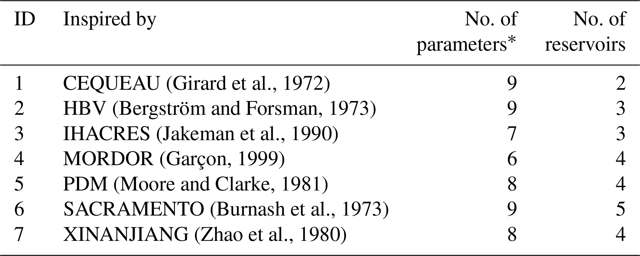
^* See Thiboult et al. (2019) and references in the second column for additional information on model parameters.

Hydrologic models are calibrated according to an asynchronous modelling framework, i.e. being forced with raw climate model outputs and excluding the day-to-day temporal correlation (Ricard et al., 2019). The calibration loop is run from 1970 to 1979 with the shuffle complex evolution algorithm (Duan et al., 1993) using 10 complexes. A 10-year period is usually considered sufficiently long for calibration, offering a sound trade-off between identifying representative parametric values and computational requirements.

3.3 Conventional hydroclimatic modelling

The proposed asynchronous workflow is compared to a conventional top-down hydroclimatic modelling approach. The latter is typically implemented to produce hydrologic scenarios from GCM or RCM simulations following three main steps (e.g. Poulin et al., 2011; Seiller and Anctil, 2014; Seo et al., 2016). Raw climate model outputs are first post-processed to correct systematic errors (or biases) according to available meteorological observations or a reference product describing the climate system over a recent and sufficiently long past period. Simulated 2 m minimum and maximum air temperature and precipitation are corrected using a quantile mapping approach (Lucas-Picher et al., 2021) combined with daily local intensity scaling (Schmidli et al., 2006). Quantile mapping is implemented every month using 100-node transfer functions interpolated linearly. The wet-day frequency is corrected using a 0.1 mm threshold. Hydrologic models are calibrated separately, forced with gridded meteorological observation datasets to optimize the performance of the simulated hydrologic response according to available streamflow observations. Hydrologic scenarios are finally constructed by forcing the calibrated hydrologic models with post-processed climate model outputs. For the sake of comparison, hydrologic modelling within the conventional hydroclimatic approach is implemented equivalently to the asynchronous workflow as described in Sect. 3.2, using the same pool of hydrologic models and calibrated parameters and the same objective function, calibration period, and configuration of the optimization algorithm.

4 Results

4.1 Biases and projected changes in NA-CORDEX 2 m air temperature and precipitation

Figure 3 illustrates the annual cycle of the 2 m mean air temperature (2mt) simulated by the nine NA-CORDEX simulations from 1970 to 1999. Only sub-catchment 2 is shown, considering that it represents most of the area of the Chaudière River catchment, but also because sub-catchments 3 and 4 are nested within. Corresponding observations issued by interpolation of in situ measurements and biases are also illustrated. Most climate simulations overestimate 2mt from November to March, the median bias of the ensemble reaching roughly +5 ^∘C in January. NA-CORDEX simulations generally provide a reasonable representation of temperature from May to September, individual biases then ranging from −2 to +2 ^∘C from one simulation to another. 2mt biases appear to be linked to the forcing GCM simulations. CanESM2-driven simulations (crx1 to crx3) lead to similar annual profiles marked by an alternation of high warm winter biases and subsequent moderate warm summer biases. EC-EARTH-driven simulations (crx4 and crx5) show a similar annual profile to CanESM2 but are affected by marked cold spring and summer biases, reaching −5 ^∘C in April in the case of crx4. GFDL-ESM2M-driven simulation (crx6) is affected by a quasi-systematic cold bias. MPI-ESM-LR-driven simulations (crx7 to crx9) finally show a constant cold bias from May to November. The winter warm bias carried by crx7 (CRCM5-UQAM, positive) differs however from the winter cold biases of crx8 and crx9 (RegCM4 and WRF).

Figure 4 illustrates the mean annual cycle of the precipitation simulated by the nine NA-CORDEX simulations from 1970 to 1999 over sub-catchment 2. The ensemble mean overestimates precipitation by roughly +0.5 mm d⁻¹ (∼ +27  %). In contrast to 2mt, biases in precipitation are fairly constant throughout the whole annual cycle, except for a brief period in autumn (August to October) when simulations are less biased. Biases typically range between −1 and +2 mm d⁻¹ depending on the period of the year. Part of the wet bias in winter precipitation can be explained by solid precipitation undercatch, which can reach 20  % to 70  % (Pierre et al., 2019). Also, in contrast to 2mt, biases in annual profiles are not as clearly related to the driving GCM.

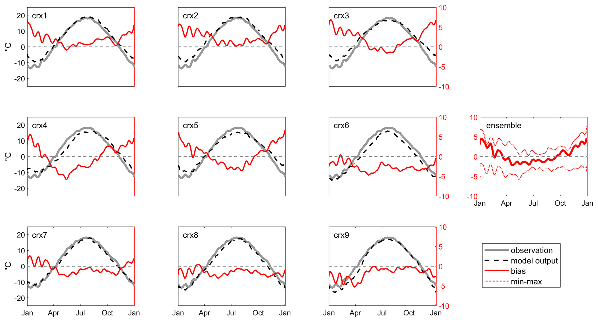
Figure 3 The 2 m mean air temperature annual cycle simulated by the nine NA-CORDEX simulations (crx1 to crx9) for sub-catchment 2, from 1970 to 1999. Observations and biases are presented. The left scale of the y axis refers to observations and raw climate model outputs and the right scale to biases. A 5 d moving window is applied to all time series to enhance the signal-to-noise ratio. In the ensemble panel, the median, minimum, and maximum biases from the nine climate simulations are illustrated. Observations are derived from the kriging of in situ data.

Figure 4 Same as Fig. 3 but for precipitation.

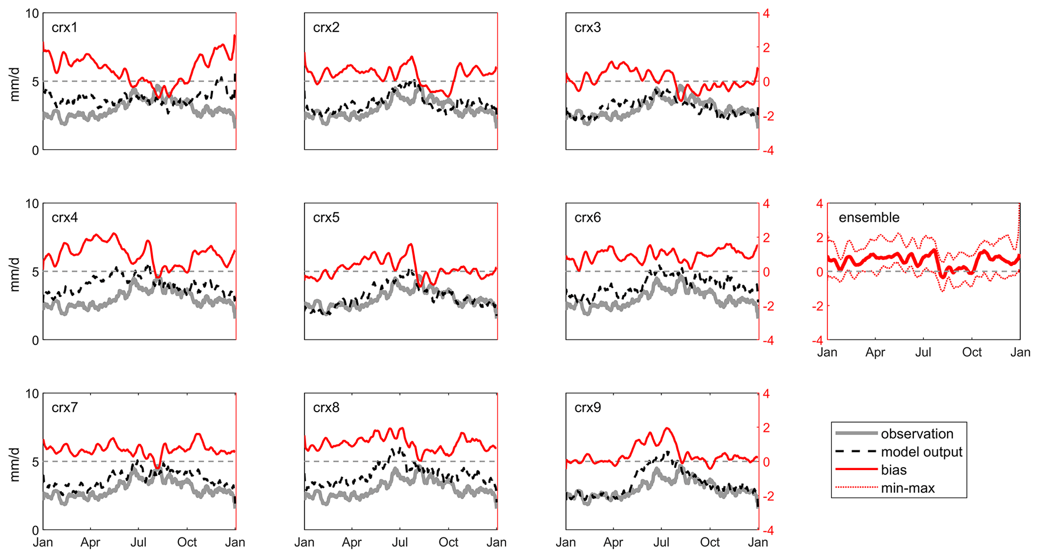
Figure 5 illustrates seasonal changes (2040–2069 relative to 1970–1999) for sub-catchment 2 for the mean 2mt and precipitation from the nine NA-CORDEX simulations. An increase in 2mt generally falls between +2 and +4 ^∘C. Also, most simulations anticipate precipitation increasing in winter (+10  % to +25  %), spring (up to +20  %), and autumn (up to +15  %) but decreasing in summer (down to −10  %). Some simulations reveal outlying trends, especially crx3 and crx4, which display, respectively, a +44  % increase in winter precipitation and almost no change in 2mt from September to November.

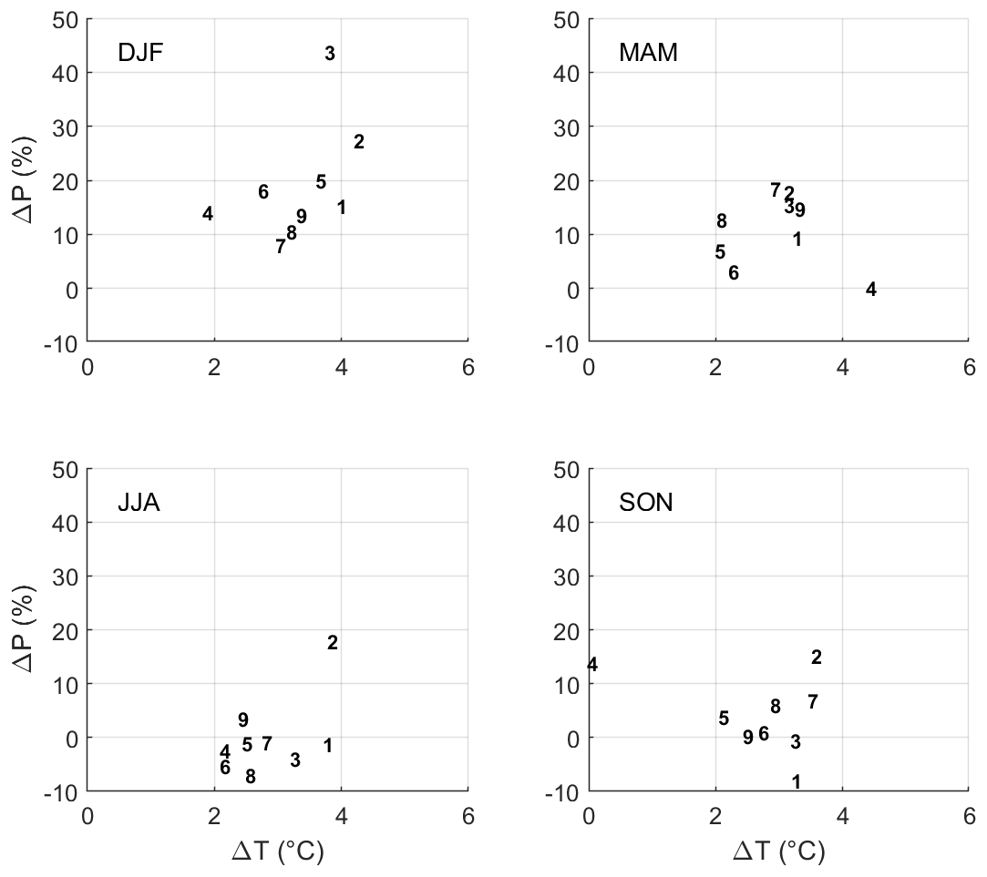
Figure 5 Projected changes (2040–2069 with respect to 1970–1999) in mean 2mt and precipitation from the nine NA-CORDEX simulations for winter (DJF), spring (MAM), summer (JJA), and autumn (SON) for sub-catchment 2. The numbers refer to the crx simulation described in Table 1.

4.2 Assessment of the asynchronous modelling workflow

Figure 6 displays the observed mean annual hydrographs at site 2 over a recent past reference period (1970–1999). The hydrograph shows typical seasonal fluctuations marked by spring flood (∼ 9.5 mm d⁻¹) in April and a second peak (much smoother, ∼ 1.8 mm d⁻¹) in November. Figure 6 also compares mean annual hydrographs simulated by the asynchronous framework and the conventional hydroclimatic approach for each NA-CORDEX simulation. The results show the capacity for the conventional approach to provide a more accurate representation of seasonal streamflow fluctuations over the reference period. Although slightly delayed and underestimated, the peak flow simulated in spring by the conventional approach is typically more accurately synchronized with observations relative to the asynchronous workflow. The inter-model variation (indicated by the envelopes in Fig. 6) related to the conventional approach also tends to be smaller and more centred around the observations, noticeably during summer, autumn, and winter. The shape of the simulated hydrographs remains finally quite similar from one NA-CORDEX simulation to another.

Hydrographs simulated by the asynchronous workflow are in some cases affected by notable flaws in representing seasonal streamflow fluctuations. The shape of the simulated hydrographs also differs notably from one NA-CORDEX simulation to another. This can be related to biases affecting raw forcing NA-CORDEX simulations (see Figs. 3 and 4). In many cases (crx4, crx6, crx8, and crx9), the spring flood is notably delayed and occurs in late spring. This could be explained by cold biases affecting simulated air temperature in spring, combined in some cases with an overestimation of solid precipitation in winter. The inter-model variation also tends to be larger relative to the conventional approach, more noticeably during summer and autumn (crx1, crx2, crx3, and crx5), but also in winter (crx1).

Hydrographs simulated at sites 1, 3, and 4 are given in Appendix A and lead to equivalent conclusions. Hydrographs simulated by the conventional approach at site 3 however produce an atypical two-fold spring flood that can be related to a specific hydrologic model. The inter-model variability is also more marked in the case of site 4 for the asynchronous framework.

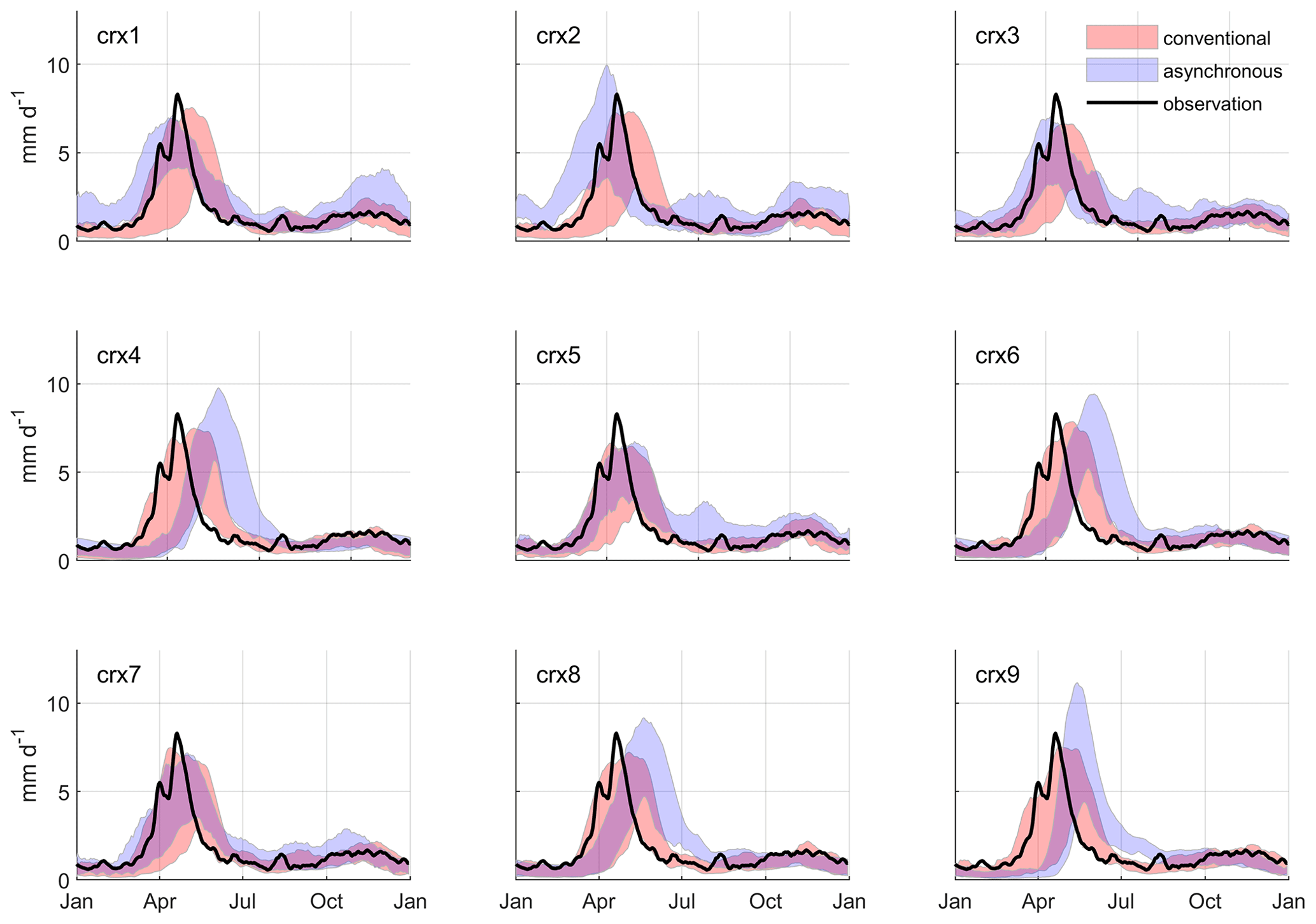
Figure 6 Mean annual hydrographs simulated at site 2 over the reference period (1970 to 1999) for each NA-CORDEX simulation. Hydrographs produced by the conventional hydroclimatic modelling approach are compared to those produced by the proposed asynchronous workflow. Envelopes refer to the 10th and 90th percentiles out of the pool of seven hydrologic models. A 5 d moving window is applied to enhance the signal-to-noise ratio. The corresponding observations are also illustrated.

Figure 7 compares the hydrologic performance of NA-CORDEX simulations (crx1 to crx9) issued by the conventional modelling approach and the proposed asynchronous workflow at sites 1 to 4. Performance is sorted according to the root-mean-square-error (RMSE) value between simulated mean annual hydrographs and corresponding observations over the 1970–1999 reference period. The median RMSE value out of seven hydrologic model simulations is presented here. The results first confirm the systematic capacity of the conventional modelling approach to provide a more accurate representation of the inter-annual hydrograph, corresponding RMSE values ranging from ∼ 0.9 to 1.2 mm d⁻¹. The performance issued by the conventional approach is also notably comparable from one site to another. On the other hand, the asynchronous workflow produces a systematically less accurate representation of the mean annual hydrograph. The most-performing simulations (ranks 1 to 5) are affected by RMSE values ranging from ∼ 1.3 to 1.6 mm d⁻¹, which is comparably performant relative to the conventional approach. A marked degradation is however observed for other less-performing simulations (ranks 6 to 9, RMSE reaching ∼ 2.5 to 3.0 mm d⁻¹ depending on the site). Sorting NA-CORDEX simulations according to their hydrologic performance systematically points to the same discrimination between the pool of the most-performing simulations (crx1, crx2, crx3, crx5, and crx7) and the less-performing ones (crx4, crx6, crx8, and crx9).

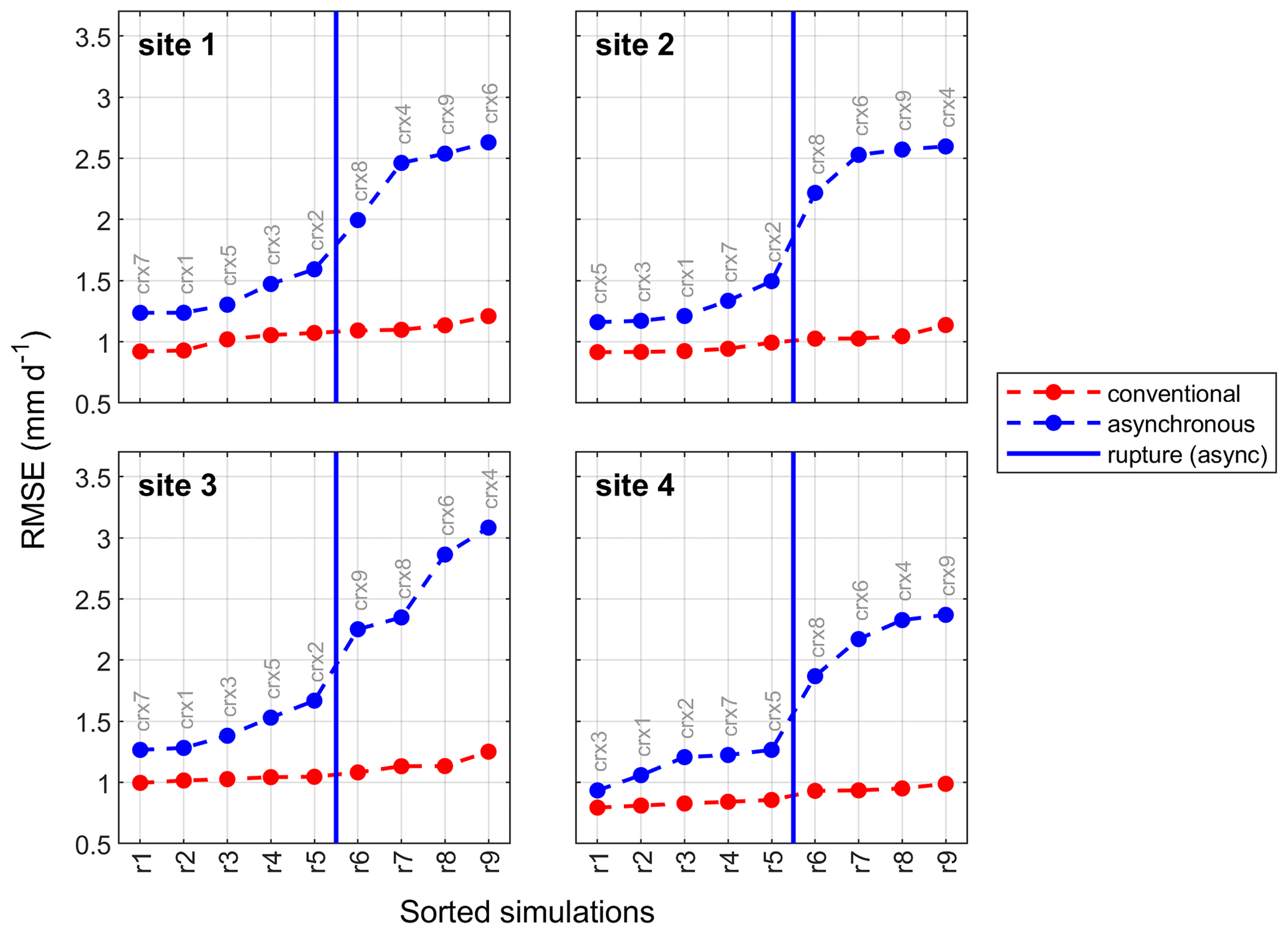
Figure 7 Sorted hydrologic performances of NA-CORDEX simulations over the reference period at sites 1 to 4 for the conventional hydroclimatic modelling approach and the asynchronous workflow. Performance is evaluated using the RMSE value between simulated mean annual hydrographs and corresponding observations. The median RMSE value out of seven hydrologic model simulations is presented here. A rupture can be observed after rank 5 for the asynchronous workflow.

Figure 8 compares projected changes in the seasonal mean flows simulated by the conventional hydroclimatic modelling approach and the proposed asynchronous workflow at sites 1 to 4. Changes are expressed in relative terms (percentage) for the nival (DJFMAM) and pluvial (JJASON) regimes and are grouped according to the driving NA-CORDEX simulation (boxes). The top five most-performing NA-CORDEX simulations identified for the asynchronous workflow are highlighted in blue. A group of outlying changes (all related to hydrologic model 1) projected by the conventional approach at site 3 is also identified in red. NA-CORDEX simulations being analysed separately, Fig. 8 shows discrepancies in change values from one modelling approach to another. Site 2 being given as an example, the spread of changes projected by crx2 is noticeably reduced using the asynchronous workflow in comparison to the conventional approach. A shift in the projected direction of change for the pluvial mean flow (Δ_JJASON) can also be observed, from a plausible decrease in the case of the conventional approach to a very likely increase for the asynchronous workflow. On the other hand, Fig. 8 also shows that both approaches lead to comparable interpretation if the projected changes are analysed as an ensemble. Site 2 once again being given as an example, both approaches strongly agree in projecting an increase in the nival mean flow (Δ_DJFMAM). Both approaches also agree in projecting a decrease in the pluvial mean flow (Δ_JJASON), except for a portion of projections mostly related to the crx2 simulation. The fact that the interpretation of the projected changes remains equivalent for both approaches can be generalized to all the sites.

Figure 8 shows that the asynchronous workflow tends to provide more outlying changes values in comparison to the conventional approach. For all the sites, numerous projections indicate very strong increases in the nival mean flow (Δ_DJFMAM), reaching up to ∼ +100  %. Such outlying projected changes are however systematically related to the less-performing NA-CORDEX simulation identified in Fig. 7. The sub-ensemble of change values resulting from the selection of the most-performing simulations (blue boxes) provides a reliable interpretation of the hydrologic changes with regard to the conventional approach, here considered the benchmark. The conventional approach can also produce notable outlying change values of nival mean flow in the specific case of site 3, all related to hydrologic model 1. Changes in the seasonal high flows and low flows projected by both approaches are presented in Appendix B.

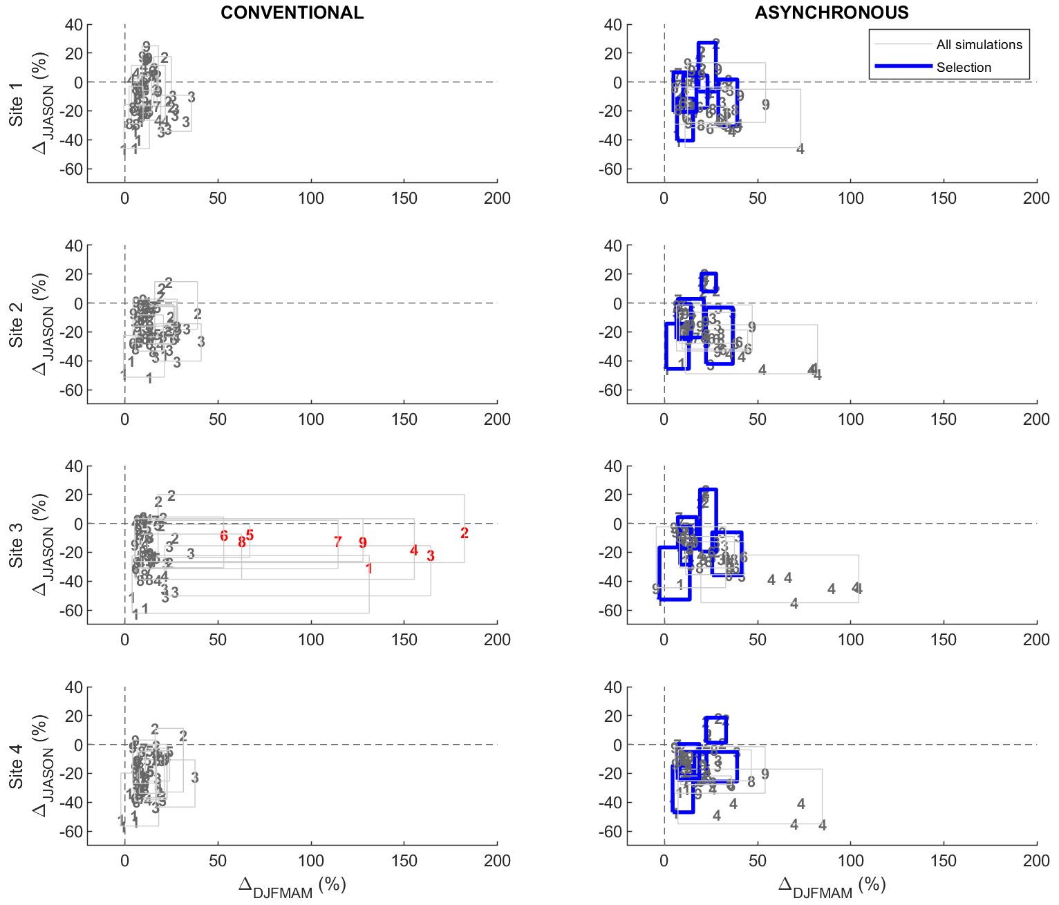
Figure 8 Changes in seasonal mean flows (Δ_DJFMAM vs. Δ_JJASON) projected for sites 1 to 4 by the conventional hydroclimatic modelling approach and the proposed asynchronous workflow. Changes are expressed in terms of relative change (%) from 1970–1999 to 2040–2069. Change values are grouped according to the forcing NA-CORDEX climate simulation (boxes, crx1 to crx9). Blue boxes refer to the selection of the most-performing simulations produced by the asynchronous workflow. The red numbers refer to outlying changes projected by the conventional approach at site 3 with the hydrologic model 1.

Table 4 summarizes the distributions of change values projected by the conventional modelling approach and the proposed asynchronous workflow. Results are displayed for site 2 using six hydrological indices describing seasonal (DJFMAM vs. JJASON) mean, high, and low flow. High- and low-flow indices are computed based on annual maximal (and minimal) values considering a 2-year return period. Distributions are composed of all possible combinations between NA-CORDEX simulations and hydrologic models (n=63) for the conventional approach and by the selection of the top five most-performing simulations for the asynchronous workflow (n=35). Change distributions are described using the “direction” of change (the portion of values pointing to an increase in a given index), the median value, and its standard deviation.

The results first confirm a strong agreement between both approaches in interpreting the changes in mean flow indices, the projected increase being equivalent in terms of direction (98 % vs. 100 %), median values (+15 % vs. +16 %), and standard deviation (9 % vs. 8 %). Both approaches also agree, but to a lesser extent, on the projected decrease in pluvial mean flow. The direction (10 % vs. 23 %), the median change value (−17 % vs. −10 %), and the standard deviation (14 % vs. 17 %) lead to a comparable interpretation of the change signal.

Modelling approaches do not agree as strongly in projecting high flows. While the asynchronous workflow indicates a probable increase in nival high flows (direction = 77 % and median $=+$10 %), the conventional approach rather provides a blurred signal. The direction of change (41 %) indicates a weak consensus among projections, and the median change value is small (+1 %). In this case, the standard deviation is comparable between both approaches (11 % vs. 12 %). The opposite situation is observed for pluvial high flows where the conventional approach projects a probable decrease (direction = 21 % and median = −13 %) and the asynchronous, distorted, and vague change signal (direction = 40 %, median = −2 %, standard deviation = 23 %).

Modelling approaches agree on the direction of change for low flows. They both indicate a probable increase in the nival lows flow (79 % vs. 77 %) and a probable decrease in the pluvial low flow (6 % vs. 16 %). The conventional approach however suggests a more severe increase in the nival low flow (median value $=+$56 %) relative to the asynchronous workflow (+21 %). The spread of the distribution is notably high in the case of the conventional approach (+132 %). Both approaches finally roughly agree on median change values (−18 % and −12 %) and standard deviations (18 % and 12 %) for pluvial low flows.

Table 4 Interpretation of change value distributions projected by the conventional hydroclimatic modelling approach and the proposed asynchronous framework at site 2. The analysis is conducted on seasonal (DJFMAM vs. JJASON) mean, high-, and low-flow indices. High- and low-flow indices refer to the 2-year return period maximal (minimal) annual streamflow values.

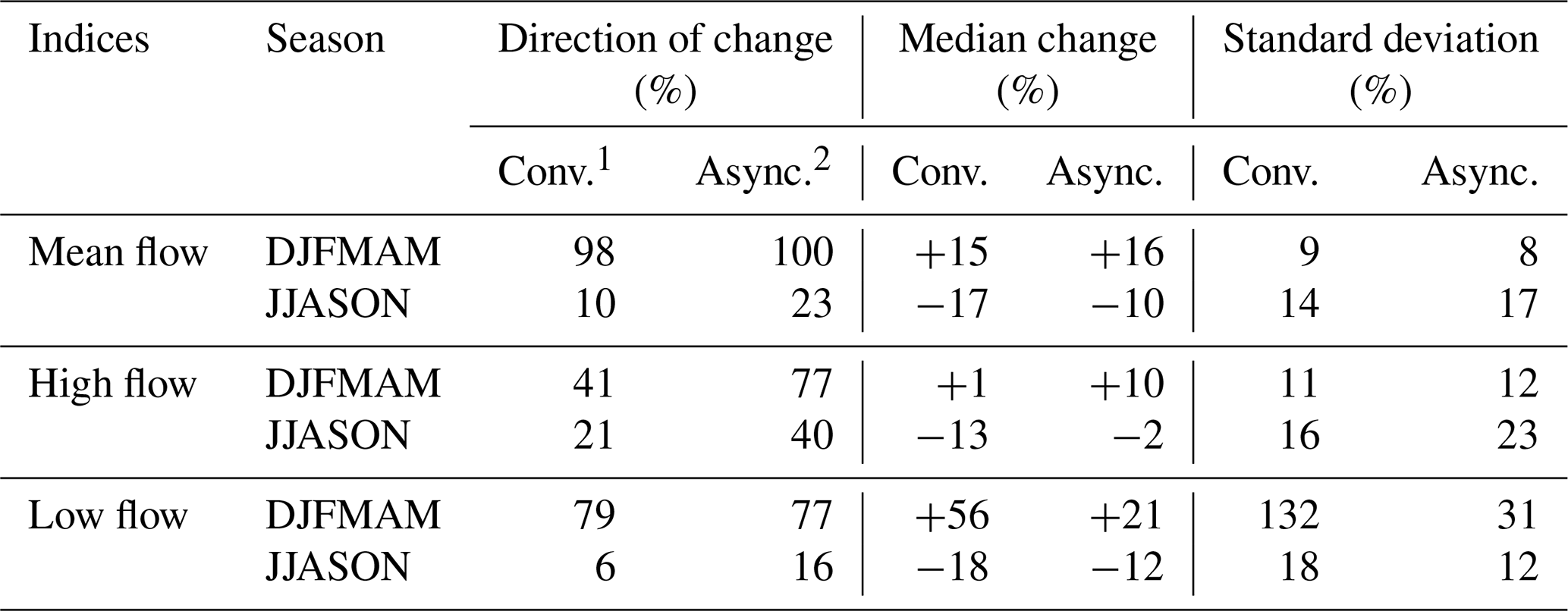
¹ All NA-CORDEX simulations (n=63). ² Selected simulations based on hydrologic performance (n=35).

4.3 Construction of hydrologic scenarios

Figure 9 illustrates change factors (ϕ) computed as prescribed by Eq. (4) issued by the asynchronous modelling framework, displayed for each streamflow quantile at site 2. Change factors are computed on an annual basis (all data, no sub-sampling of the annual cycle) and for the nival (DJFMAM) and pluvial (JJASON) regimes that both experience low- and high-flow periods. Change factors are defined from percentile 0.005 to percentile 0.995 by increments of 0.01 (100 nodes), interpolated linearly. Results are shown for all NA-CORDEX simulations and for the selected most-performing ones, respectively. Annual factors show few little projected changes in streamflow quantiles from the reference to future periods. They confirm an increase for lower quantiles (ϕ roughly ranging between 0.9 and 1.5), while no clear change signal can be observed for higher quantiles. On the other hand, nival change factors (DJFMAM) show much more marked projected changes from the reference to the future. While all simulations agree on an increase for smaller streamflow quantiles (ϕ ranging between 1 and 2), ϕ reaches the value of 2.9 for quantile 0.8. ϕ abruptly decreases for quantiles above 0.9, ranging between 0.9 and 1.3. Pluvial change factors (JJASON) are not as marked as nival factors. They confirm however a consensual decrease for quantiles below 0.8. The consensus weakens for higher quantiles, corresponding ϕ values being centred around 1 and affected by a larger spread. One must notice that the selection of NA-CORDEX simulations based on hydrologic performance typically agrees with the ensemble composed by all simulations, except for projecting a nival streamflow quantile from 0.5 to 0.9. In this case, the selected simulations provide a much smaller increase in nival high flows, ϕ typically being below 1.5.

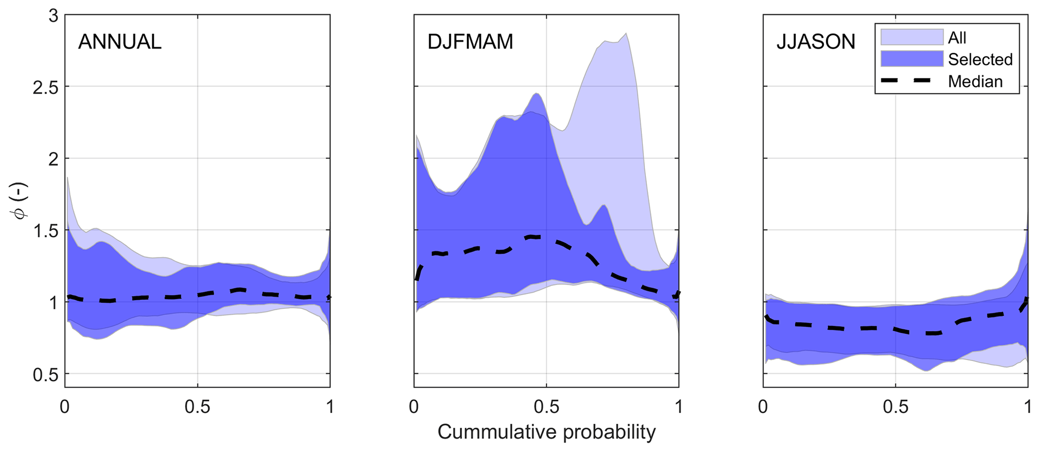
Figure 9 Streamflow change factors (ϕ) from the reference period (1970–1999) to the future (2040–2069) issued by the asynchronous modelling workflow at site 2. Factors are computed on annual and seasonal (DJFMAM vs. JJASON) bases. They are also presented for all NA-CORDEX simulations and for the top-five selection of simulations based on hydrologic performance. Envelopes refer to the 10th and 90th percentiles. The median of the selected ensemble is also shown.

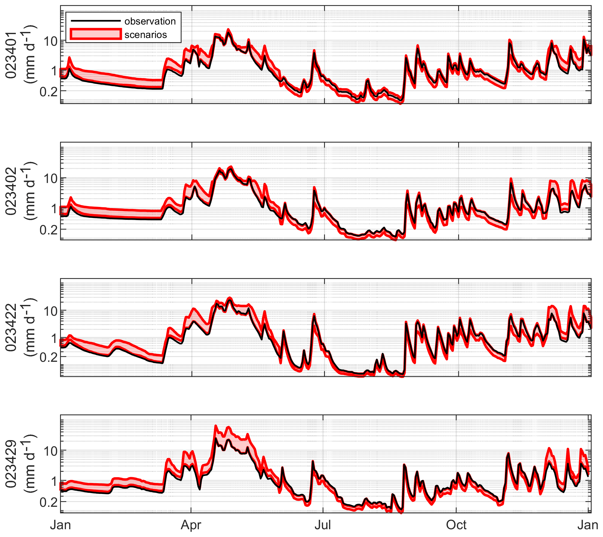
Figure 10 Hydrologic scenarios (in red) produced by applying quantile perturbation to streamflow observations (in black) for each Chaudière River sub-catchments (sites 1 to 4) for 1982 (given as an example). The min-max red envelope refers to the nine scenarios issued by the raw NA-CORDEX simulations. Note the log axis on the y axis.

Figure 10 displays the hydrologic scenarios over the 2040 to 2069 period according to RCP8.5, produced over the Chaudière River sub-catchments by applying the quantile perturbations to the observed streamflows. Observed and projected hydrographs are shown for the selected year 1982, given as an example. The hydrologic scenarios reflect the relative changes embedded within the distributions of change factors shown in Fig. 9. Future winter low flows are systematically higher relative to the observations. Mid-amplitude spring high flows are also affected by notable increases, which is not systematically the case for high-amplitude peak flows. Summer low flows tend to decrease, while summer and autumn high flows are affected by moderate increases and decreases, depending on the climate scenario.

5 Discussion

5.1 A complement to conventional hydroclimatic modelling

Nowadays, the quantification of climate change impacts on water resources mostly resorts to the implementation of top-down modelling cascades, translating climate model outputs into simulated hydrologic time series at the catchment scale. Typically, a statistical post-processing is applied to the raw climate model outputs in order to reduce biases imbedded in the simulated climate variables. Hydrologic models are also typically calibrated when forced by meteorological observations aiming to identify optimal parameter sets minimizing errors between simulated and observed discharge at a given catchment outlet. Assessing the impact of climate change on the hydrologic regime of a catchment using this conventional modelling approach presents drawbacks documented in the scientific literature: (1) the statistical post-processing of climate model outputs may disrupt the physical consistency between the simulated climate variables and even alter the corresponding trends from a reference period to a future period, (2) the modelling work flow relies highly on the availability and quality of meteorological observations in order to conduct the statistical post-processing of climate model outputs and the calibration of the hydrologic model, and (3) it also requires a high level of expertise and computing capacities to post-process the outputs and uses non-trivial statistical methods, restraining the participation of end-users in interpreting and attributing confidence in the simulation results.

In this study, we propose a simplified modelling workflow that enables the production of hydrologic scenarios without resorting to the statistical post-processing of climate model outputs. This asynchronous approach is conducted by calibrating the hydrologic model forced directly with raw climate model outputs instead of meteorological observations, using an objective function that excludes the temporal correlation between the observed and simulated hydrologic responses. Calibrated hydrologic models allow for the conversion of a raw climate model into corresponding reference and future simulated hydrologic responses. Hydrologic scenarios are subsequently produced by applying quantile perturbations to available streamflow observations, with the perturbation factors identified by relating simulated reference and future hydrologic responses for each streamflow quantile. Quantile perturbation is applied to simulated climate variables such as precipitation or reference evapotranspiration (Ntegeka et al., 2014) but never, to our knowledge, to the simulated hydrographs resulting from a hydroclimatic modelling cascade. To our knowledge, two approaches help preserve the physical consistency of climate model outputs and their trends: to apply trend-preserving multi-variate methods or to use raw model outputs straightforwardly for impact analyses, accepting biases. The proposed asynchronous framework is based on calibrating a hydrologic model using raw model outputs, assuming a consistent relative change (within climate simulations) from the reference to future periods. We acknowledge (and discuss below) the requirement for calibration as a limitation of the proposed framework, considering that it may disrupt the consistency of simulated hydrologic processes at the catchment scale.

We assessed the proposed asynchronous workflow by comparing its projected hydrologic regime with a conventional hydroclimatic modelling approach. As shown by others (e.g. Muerth et al., 2013), our results confirmed that the post-processing of raw climate model outputs increases the performance of the simulated hydrologic response over the historical reference period. On the other hand, our results demonstrated that the projected changes in the seasonal mean flows, taken as ensembles, converged to equivalent conclusions, regardless of the chosen modelling approach. The concordance between both approaches did not occur as sharply for high- and low-flow indices, suggesting that further investigations would be required to clarify how and to which extent the projection of high- and low-flow events is sensitive to the selection of the hydroclimatic modelling approach. We here emphasize the fact that the asynchronous workflow is vulnerable to strong biases affecting raw climate model outputs and is consequently more prone in producing outlying projections of hydrologic indices. However, the performance of the simulated response over the reference period provided a functional criterion to identify less-performing NA-CORDEX simulations. Based on the results shown in Sect. 4, we would advocate for the exclusion of these simulations for the analysis of the simulated projections of the hydrologic regime using an asynchronous modelling framework.

Although the proposed asynchronous framework does not completely solve the weaknesses of the traditional modelling approach, it presents the following benefits. (1) It increases confidence in the hydrologic scenarios since it is conducted with raw climate model outputs, thus preserving physical consistency between simulated climate variables and original trends simulated by the climate models (although it requires the calibration of a hydrologic model discussed below) – some authors also foresee that raw climate model outputs will improve in resolution and reliability with time (e.g. Teng et al., 2015; Chen et al., 2017). (2) It does not resort to meteorological observations, not for operating statistical post-processing or for calibrating the hydrologic model, facilitating the assessment of climate change impact on water resources for regions afflicted by observation scarcity (a significant benefit since most of the earth system is affected by data scarcity) – we would also argue that our approach does not inject uncertainty into the modelling cascade from the intrinsic limitations of post-processing methods (Laux et al., 2021) or from poor-quality observations or reference products describing the reference climate system (Hwang et al., 2014; Kotlarski et al., 2017). (3) It is simple to implement and is lighter in computing requirements – post-processing is exclusively applied to streamflow instead of numerous climate variables.

We believe however that the proposed workflow should be used wisely in areas where meteorological observations are abundant and reliable, rather as a complement to than as a substitute for conventional hydroclimatic modelling. In such cases, we would definitively encourage a sound use of all meteorological observations.

Further works could explore the use of bias correction within the asynchronous workflow, aiming to maximize the use of observations while producing hydrologic scenarios at the regional scale or modelling more complex physical processes at the catchment scale. Another assessment scheme could compare the performance of both modelling frameworks with intentionally degraded (scarcer) forcing data. Such comparison could confirm under which conditions the use of a given framework would be preferable over another.

5.2 A bottom-up perspective

Statistical post-processing of climate model outputs implies a necessary trade-off between key methodological benefits and drawbacks in the scope of providing reliable and supportive information for adaptation to climate change. On the one hand, simulated climate variables are corrected to fit statistical properties of the observed climate system. On the other hand, statistical post-processing disrupts physical consistency and alters trends in the simulated climate variables. While designing statistical post-processing, a decision is implicitly taken on how these benefits and drawbacks are weighted. In a pure top-down perspective, statistical post-processing is applied according to climate-oriented prerogatives, the end-user rarely being involved in deciding upon which benefit to be prioritized and which drawbacks to be limited. Moreover, not communicating source biases affecting raw climate model outputs constrains the capacity of impact modellers and end-users have in assessing the climate model representativeness and attributing confidence to resulting climate scenarios. Nowadays, solutions explored by the scientific community mostly resort to the development of sophisticated post-processing methods. Even though such approaches present undeniable benefits in terms of post-processed physical consistency and trend preservation, we would argue that they further enlarge the gap between climate specialists and water resource end-users.

The approach proposed in this study remains in essence a top-down modelling workflow. Through notable simplifications and straightforward constructions between raw climate model outputs and impact models, this alternative framework creates a space for an increased participation of climate model experts, impact modellers, and end-users in interpreting climate change impacts on water resources (Ehret et al., 2012). It is thus compatible with integrated and transdisciplinary environmental assessments and modelling frameworks in support of decision and policy making (Hamilton et al., 2015; Rössler et al., 2019). By translating raw climate model outputs into the corresponding simulated hydrologic responses, the representativeness of climate models can be assessed in a language further understandable for impact modellers and end-users. Based on the simulated hydrologic responses over the reference period (see Mudbhatkal and Mahesha, 2018), key methodological questions can be addressed and debated through an open and empowered dialogue with climate specialists. These questions can be the following.

• Are climate model outputs representative enough to assess the impacts of climate change on water resources?

• Should the climatic or hydrologic representation be prioritized, or both?

• How should less representative simulations be treated: rejected, weighted (e.g. Shin et al., 2020), or considered equal?

• Are scenarios required for the adaptation to climate change, or are relative change signals sufficient?

• Should post-processing be applied to raw climate model outputs?

We believe that decisions on such questions require a sound understanding of simulated climate forcing but also an in-depth awareness of the local specificities of the hydrologic system exposed to climate change. Considering the above arguments, one could rather use the proposed asynchronous workflow as a hybrid analytical framework to evaluate the vulnerability of water resource systems instead of as a pure top-down predictive assessment tool.

5.3 Limitations

The assessment of the proposed asynchronous workflow indicated that the simulated hydrologic response is affected by systematic errors (or hydrologic biases), mostly notable in terms of synchronism of the mean annual hydrograph during spring flood. Considering this, we would advocate that the proposed workflow should be used with caution when focusing on analysing high- and low-flow events. To formally assess the impact of climate change on a given domain, however, a larger ensemble of climate simulations should be considered. Since the workflow does not involve statistical processing of climate model outputs, we would recommend the use of high resolution over coarse gridded climate simulations in order to rely on an improved representation of local-scale processes. The use of seven conceptual lumped hydrologic models can also be considered a limitation to our approach. Although they provide a diversity in modelling structure, no formal evaluation of this specific source of uncertainty has been considered in this study (calibration metric, calibration period, structure complexity).

Assessing the impact of climate change on water resources within the proposed framework implies that the resulting hydrologic scenarios are inevitably tainted by (hydrologic) biases. These biases emerge from raw climate model outputs but also from the limitations imposed by the structures of the hydrologic models. We believe that further work should focus on evaluating how these two sources are intertwined. We also acknowledge that the proposed approach may disrupt the physical consistency of the processes simulated at the catchment scale through parametric compensation affecting the calibration of the hydrologic model. Further work is required to assess how parametric compensation may affect the trade-off between hydrologic scenarios fitted to observations and the preservation of the hydrologic change signal embedded within raw climate model outputs. Such analysis could also clarify the impact of parametric compensation relative to bias correction of raw climate model outputs. In the meantime, we would argue that parametric compensation should be minimized as much as possible to preserve the hydrologic change signal. This could be achieved, for example, by restraining parametric spaces during calibration as closely as possible to realistic boundaries or favouring physically based descriptions of hydrologic processes. Even if climate models constantly improve, their biases can still be important, and a judgement must be made in order to attribute confidence to the resulting hydrologic scenarios. Chen et al. (2021) explicitly raised the idea of an optimal selection of climate simulations before producing hydrologic scenarios to cope with their limitations in representing local hydrometeorological patterns. We do not propose here any specific guidelines, except that such an attribution must consider the scope and objectives of the conducted study and should involve, as much as possible, climate specialists, impact modellers, and end-users.

The proposed workflow is not limited by available meteorological observations, but to available streamflow observations. To assess the impact of climate on ungauged water resources, modellers can translate the hydrologic perturbation signals under the assumption of representativity of available discharge observation with regards to the ungauged domain. If ungauged streamflow is estimated before applying a change factor (using area ratio, hydrological modelling, or optimal interpolation), the corresponding uncertainties must by considered.

Constructing hydrologic scenarios using quantile perturbations, our results demonstrated the necessity of identifying a suitable time period to define change factors. Such resolution must consider specificities of the local flow regime magnitudes. The identification of an optimal duration remains an open question, keeping in mind that the use of a moving window could become necessary to compensate for a breakpoint in the hydrologic scenarios. We acknowledge that the quantile perturbation assumes a comparison between two stationary periods (reference vs. future) and does not consider potential rupture in future trends. We believe that shifts in the seasonal cycle could theoretically be more precisely assessed by applying sub-annual perturbation factors. Even considering the relative change for each streamflow quantile, the capacity of quantile perturbation to preserve mean flows and seasonal budgets should be explored and assessed further.

6 Conclusion

This study explores an innovative and straightforward hydroclimatic modelling workflow enabling the construction of hydrologic scenarios without meteorological observations. Hydrologic models are forced with raw climate model outputs and calibrated using an objective function that excludes the day-to-day temporal correlation between simulated and observed hydrographs. Hydrologic scenarios are produced by applying quantile perturbation to the available observed streamflow measurements. This workflow is implemented over a mid-scale catchment located in southern Quebec, Canada, using an ensemble of NA-CORDEX simulations and a pool of lumped conceptual hydrologic models. The asynchronous workflow is assessed by comparing its resulting projections of hydrologic indices with a conventional hydroclimatic modelling approach. The latter involved post-processing of raw climate model outputs and calibration of hydrologic model using meteorological observations. Results showed that both methods lead to equivalent projections of the seasonal mean flow indices. Both approaches did not agree as well in projecting high- and low-flow indices, suggesting that further works should be conducted to confirm the reliability of the proposed workflow to assess the impact of climate change on high- and low-flow events. The results also highlight the importance of considering seasonal fluctuations of the hydrologic regime while applying quantile perturbations to the observed streamflow measurements. We argue that the suggested workflow increases the confidence attributed to the hydrologic scenarios, mostly because it preserves physical consistency between driving simulated climate variables. We also underline that the workflow eases communication between climate experts, impact modellers, and end-users, thus supporting decision-making in the process of the adaptation of water usages to climate change.

Appendix A

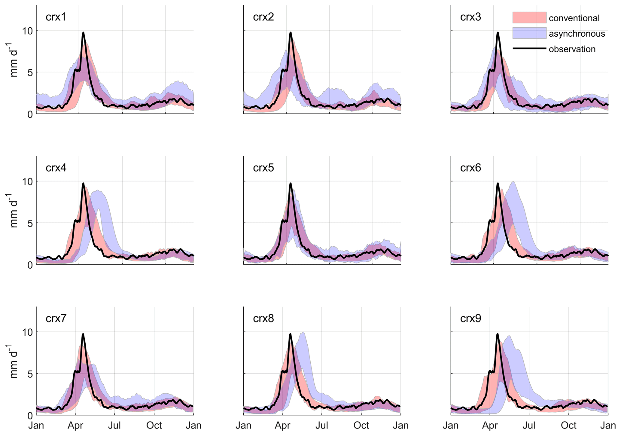
Figure A1 Mean annual hydrographs simulated at site 1 over the reference period (1970 to 1999) for each NA-CORDEX simulation. Hydrographs produced by the conventional hydroclimatic modelling approach are compared to those produced by the proposed asynchronous workflow. Envelopes refer to the 10th and 90th percentiles out of the pool of seven hydrologic models. A 5 d moving window is applied to enhance the signal-to-noise ratio. The corresponding observations are also illustrated.

Figure A2 Same as Fig. A1 but for site 3.

Figure A3 Same as Fig. A1 but for site 4.

Appendix B

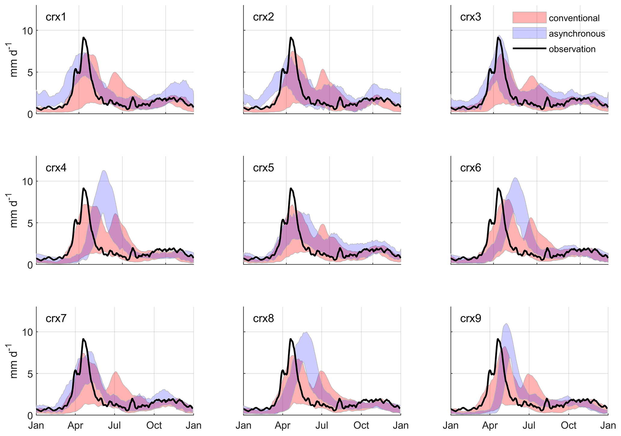
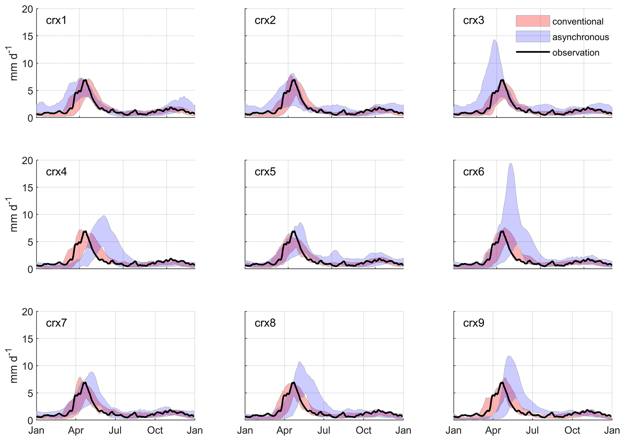
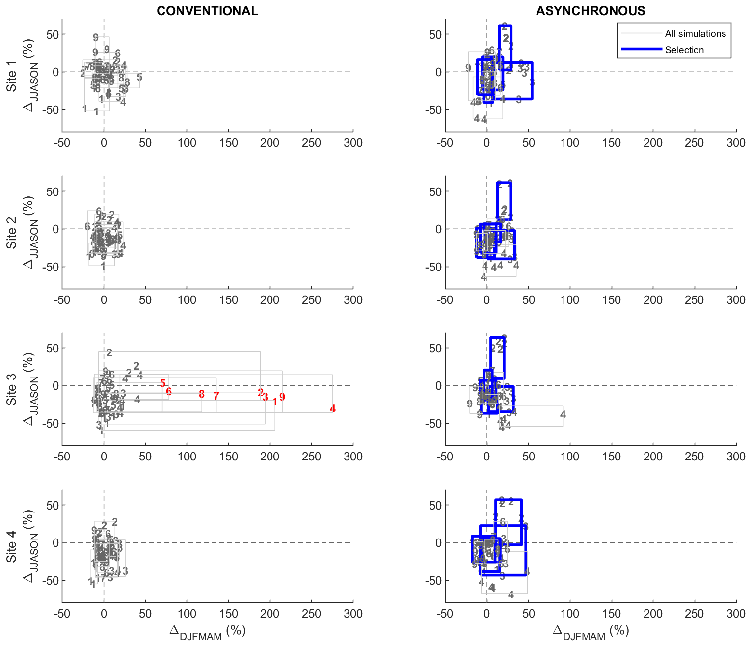
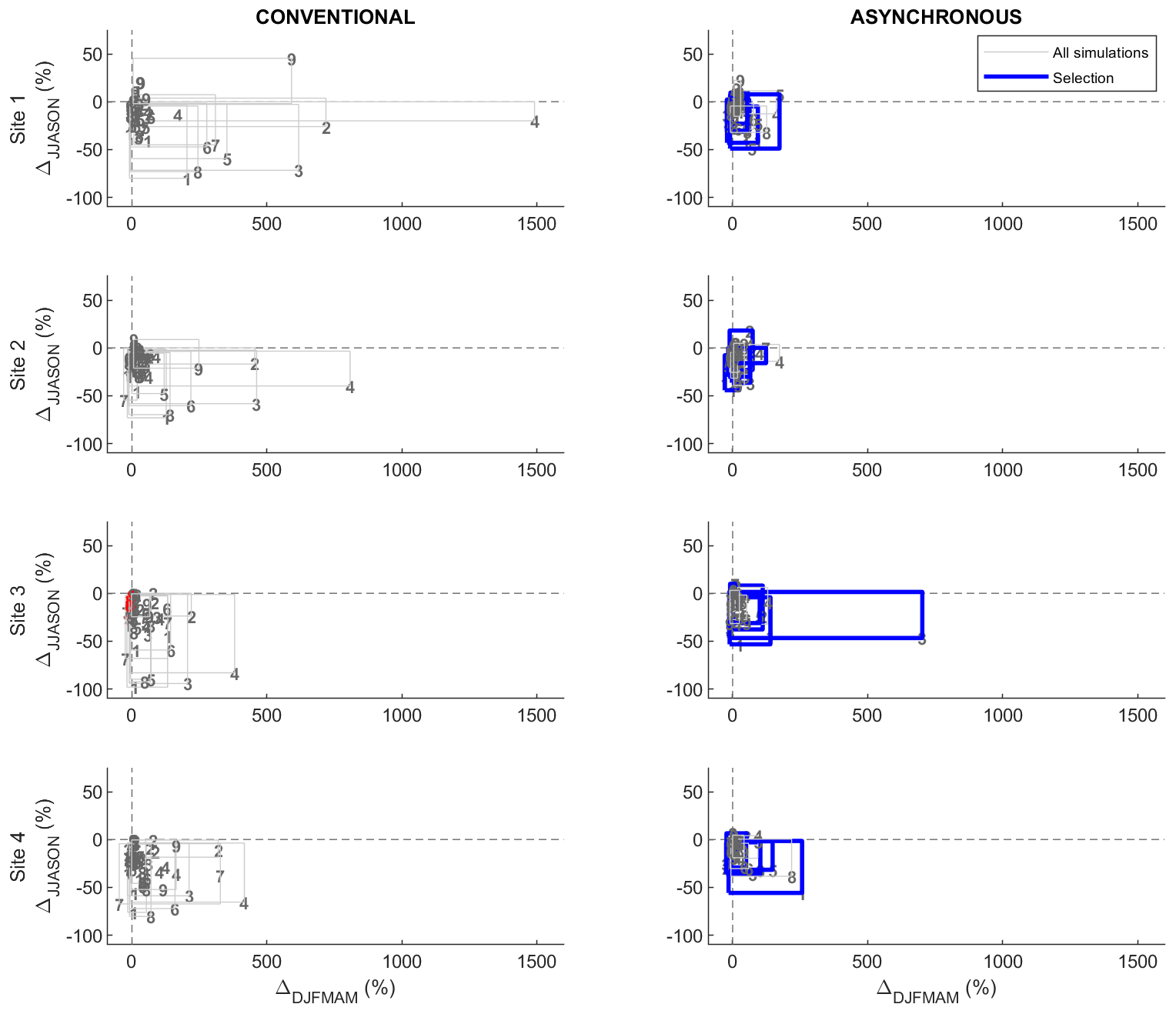
Figure B1 Changes in seasonal high flows (Δ_DJFMAM vs. Δ_JJASON) projected for sites 1 to 4 by the conventional hydroclimatic modelling approach and the proposed asynchronous workflow. High flows are computed based on the annual maximal value with a 2-year return period. Changes are expressed in terms of relative change (%) from 1970–1999 to 2040–2069. Change values are grouped according to the forcing NA-CORDEX climate simulation (boxes, crx1 to crx9). Blue boxes refer to the selection of the most-performing simulations produced by the asynchronous workflow. The red numbers refer to outlying changes projected by the conventional approach at site 3 with the hydrologic model 1.

Figure B2 Same as Fig. B1 but for low flows.