Snow data assimilation for seasonal streamflow supply prediction in mountainous basins

Accurately predicting the seasonal streamflow supply (SSS), i.e., the inflow into a reservoir accumulated during the snowmelt season (April to August), is critical to operating hydroelectric dams and avoiding hydrology-related hazard. Such forecasts generally involve numerical models that simulate the hydrological evolution of a basin. The operational department of the French electric company Electricité de France (EDF) implements a semi-distributed model and has carried out such forecasts for several decades on about 50 basins. However, both scarce observation data and oversimplified physics representation may lead to significant forecast errors. Data assimilation has been shown to be beneficial for improving predictions in various hydrological applications, yet very few have addressed the seasonal streamflow supply prediction problem. More specifically, the assimilation of snow observations, though available in various forms, has been rarely studied, despite the possible sensitivity of the streamflow supply to snow stock. This is the goal of the present paper. In three mountainous basins, a series of four ensemble data assimilation experiments – assimilating (i) the streamflow (Q) alone, (ii) Q and fractional snow cover (FSC) data, (iii) Q and local cosmic ray snow sensor (CRS) data and (iv) all the data combined – is compared to the climatologic ensemble and an ensemble of free simulations. The experiments compare the accuracy of the estimated streamflows during the reanalysis (or assimilation) period September to March, during the forecast period April to August, and the SSS estimation. The results show that Q assimilation notably improves streamflow estimations during both reanalysis and the forecast period. Also, the additional combination of CRS and FSC data to the assimilation further ameliorates the SSS prediction in two of the three basins. In the last basin, the experiments highlight a poor representativity of the CRS observations during some years and reveal the need for an enhanced observation system.

1 Introduction

Accurately predicting the seasonal streamflow supply (SSS), i.e., the inflow into a reservoir accumulated during the snowmelt season (April to August), is critical to operating hydroelectric dams and avoiding hydrology-related hazard. Hence, the operational department of the French electric company Electricité de France (EDF) has been carrying out such forecasts for several decades for nearly 50 basins. However, in mountainous basins, the confidence provided by long-term hydrological forecast is affected by the uncertainty in the meteorological forcings (Li et al., 2009; Bormann et al., 2013; Luce et al., 2014) and the inaccurately simulated snowpack (Liston and Sturm, 1998; Pan et al., 2003). Acknowledging that the SSS partly depends on the snowpack accumulated during winter, the growing number of satellite observations of snow-related quantities and in situ snow measurements may open the way to improving the SSS predictions in mountainous basins.

Some studies suggest that controlling the snowpack evolution using observations can significantly ameliorate short- and long-term streamflow forecasts (Viviroli et al., 2011; Fayad et al., 2017). In the present paper, a sensitivity experiment is conducted to highlight how the uncertainties propagate within a hydrological system. The Sobol indices are computed for each of the model variables, indicating the impact that the uncertainty of these variables has on the uncertainty of the streamflow at the outlet. This experiment investigates whether a better representation of the snowpack could result in a significant gain in SSS estimation.

Data assimilation techniques are often used to help control and refine hydrological systems (see Largeron et al., 2020, for a detailed review). Several studies have successfully assimilated snow water equivalent (SWE) data but mostly in local models, i.e., models describing the snow dynamics at a specific site and not the hydrological system of an entire basin. Indeed, SWE measurements, especially from ground-based cosmic ray sensor (CRS; Kodama et al., 1979; Paquet and Laval, 2006) instruments, provide very local information which can be used to improve a local model at a specific site (e.g., Piazzi et al., 2018, at three Alpine sites). Assimilating CRS data in a basin-scale model as is can lead to representativity errors (where the SWE measured by a CRS does not correspond to any relevant global SWE model), thus deteriorating the system estimation. To circumvent this issue, an alternative approach to consider CRS data in a basin-scale model is discussed in Sect. 4.3, used throughout the following experiments, and shows promising results.

Multiple studies have implemented ensemble-based data assimilation schemes, such as the ensemble Kalman filter (EnKF, Evensen, 2003), of direct or indirect snow observations (Andreadis and Lettenmaier, 2006; Clark et al., 2006; Slater and Clark, 2006; Su et al., 2008; Magnusson et al., 2014; Piazzi et al., 2019, 2021). However, the nonlinear nature of these snow-related observations and the complexity to control a hydrological system with indirect information seem to favor the use of a more nonlinear and non-Gaussian data assimilation method, especially when aiming at long lead-time prediction improvements (Dumedah and Coulibaly, 2013). One data assimilation method in particular, the particle filter (PF, Van Leeuwen, 2009), is known for its ability to handle highly nonlinear systems containing non-Gaussian probabilities. The PF implements Bayes' theorem by describing the probability density functions as a sum of Dirac functions from an ensemble of simulations (particles) and without any additional hypothesis. Therefore, under the assumption of a sufficiently large ensemble of particles, the PF provides the optimal solution of any inverse problem. In hydrological applications, DeChant and Moradkhani (2011) managed to improve SWE and discharge forecast using microwave radiance assimilation with a PF. Also, Leisenring and Moradkhani (2011) showed in a synthetic experiment comparing an EnKF and a PF that the assimilation of SWE data with a PF improved seasonal predictions. The work of Charrois et al. (2016) has shown the good performance of the PF for the assimilation of optical reflectivity and snow depths, and Piazzi et al. (2018) successfully used a PF for SWE data assimilation in mountainous regions. Finally, Piazzi et al. (2021) concluded that PF assimilation outperforms an EnKF assimilation by generating longer-lasting predictions.

The relevance of using local snow observations is an open question though. How much is the SSS prediction sensitive to the snowpack? Do the snow observations contain the necessary information to estimate the snowpack accurately enough to impact the quality of predictions? To answer these questions, the present paper assesses the potential of using local snow observations in a seasonal forecast procedure to improve the streamflow supply prediction at the outlet of mountain basins. This is addressed by implementing real data assimilation experiments.

The experiments performed in the present article are based on the MORDOR-SD model (Garavaglia et al., 2017), the semi-distributed version of the original MORDOR model, used by EDF for many years. The experiments have been deployed on three French mountainous basins. Three types of observations are available in these basins: the observed streamflow at the outlet Q, CRS data and fractional snow cover (FSC, Masson et al., 2018), provided by the Moderate Resolution Imaging Spectroradiometer (MODIS) satellite. Each year, an assimilation of the available data is performed from September to March of the following year. Throughout the paper, this time period is called the reanalysis (or assimilation) period. A free forecast is then run from April to August. This time period is called the forecast period. The performance of the assimilation is evaluated during both the reanalysis and the forecast period.

The paper is structured as follows: a description of the model and observations used in the study, i.e., the numerical model, the three hydrological basins and the available observations (Sect. 2), a study of the sensitivity of the system (Sect. 3), the description of the experimental protocol (Sect. 4) and the assimilation results (Sect. 5). A summary and conclusions are given in Sect. 6.

2 Model and observations

2.1 MORDOR-SD model

For many years, EDF teams have been using a hydrological box model: the MORDOR model. In this study, we use the semi-distributed MORDOR-SD model (Garavaglia et al., 2017), which is an improvement on the original MORDOR that includes a spatial discretization scheme. MORDOR-SD is based on a succession of hydrological components: the potential evaporation is determined by an evaporation function (depending on air temperature), the surface storage U (modeling a rainfall excess and soil moisture accounting storage) impacts the evaporation and the direct runoff, the capillarity storage Z is fed by indirect runoffs and also impacts the evaporation, the hillslope storage L separates direct and indirect runoffs, the rest feeds the deep storage N that provides the baseflow component and, lastly, a snow stock S is accumulating or melting based on an improved degree-day formulation. More specifically, the snow model is derived from a classical degree-day scheme, with a few important additional processes: (i) a cold content able to dynamically control the melting phase; (ii) a liquid water content in the snowpack; (iii) a groundmelt component and (iv) a variable melting coefficient, depending on the potential radiation assumed to model the changing albedo effect throughout the melting season. The accumulation phase is controlled by the discrimination of the liquid and solid fractions of the precipitations. Finally, the total runoff Q is then determined with a unit hydrograph.

The discretization scheme of MORDOR-SD is based on an elevation band approach adapted for mountain hydrology. Classically, the number of elevation bands is optimized depending on the hypsometric curve of the basin according to the following criteria: (i) the relative area of each elevation band has to be greater than or equal to 5 % and less than or equal to 50 %, and (ii) the elevation range of each zone has to be lower than 350 m.

In most MORDOR-SD applications, the spatial variability of meteorological forcing is summarized by two orographic gradients: gpz (% × 1000 m⁻¹) for precipitation and gtz (^∘C × 100 m⁻¹) for temperature (see Appendix 2 of Garavaglia et al., 2017). In this way, we assume that, in mountainous areas, spatial variability is primarily determined by elevation.

In our configuration, the MORDOR-SD model has five state variables in each elevation band: four storage water levels (U, L, Z and S) and the snowpack bulk temperature (TST). The model has one global variable N representing the deep storage water level. The number of free parameters ranges from 10 to 12 depending on the basin-specific calibration strategy. See Garavaglia et al. (2017) for a thorough description of MORDOR-SD components and flows.

In addition to the state variables, the MORDOR-SD model depends on two atmospheric forcings: temperature T and precipitation P. Both forcings result from a statistical reanalysis based on ground network data and weather patterns (Gottardi et al., 2012). The MORDOR-SD model is prescribed with the spatial average of these forcing data over the basin and are given at daily time steps. As discussed previously, the model modifies the impact of the forcings at the different elevations using two orographic gradients. The orographic gradients are constants prescribed to the model (gpz = 21 %, 39 % and 28 % × 1000 m⁻¹ and gtz = −0.75, −0.60 and −0.57 ^∘C × 100 m⁻¹, respectively, for the three basins studied in this paper and described in the next section: the Verdon, Naguilhes and Guil basins). In the rest of the work presented here, these gradients will not be discussed further; however, these vertical gradients might represent a significant source of uncertainty, and their impact should be investigated in future works.

In the following experiments, first-order stochastic autoregressive (AR1) processes are used to perturbed the atmospheric forcings. These AR1 processes introduce perturbations on the forcings that are consistent in time and that provide MORDOR-SD with an ensemble of probable meteorological scenarios. An AR1 process is added to the temperature in order to simulate the instrument and the representativity errors. The precipitation is multiplied by an AR1 (centered around 1) process, so that the variability in the precipitation intensity is simulated but no new day of precipitation created. An illustration of the ensemble of forcings generated for the year 2001 in the Verdon basin (later described in Sect. 2.2) is provided in Fig. 1. The calibration of these ensembles (i.e., calibration of the parameters of the autoregressive processes) plays a crucial role in the implementation of the assimilation system and is further discussed in Sect. 4.1.

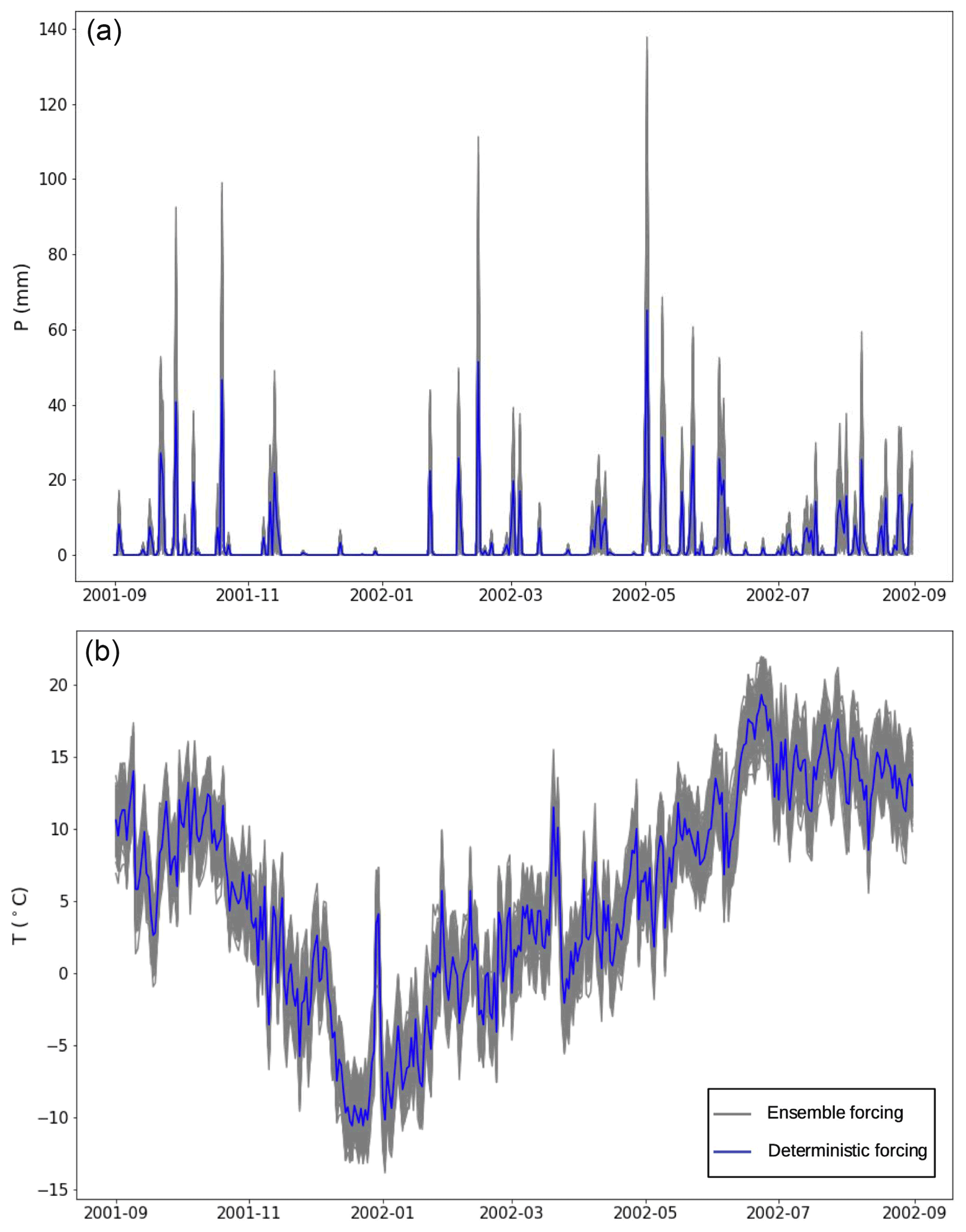
Figure 1 Time series of the forcings: precipitation P (a) and temperature T (b) during the years 2001–2002 in the Verdon basin. The deterministic forcings are represented in blue, and the corresponding perturbed 50 ensemble members are plotted in gray curves.

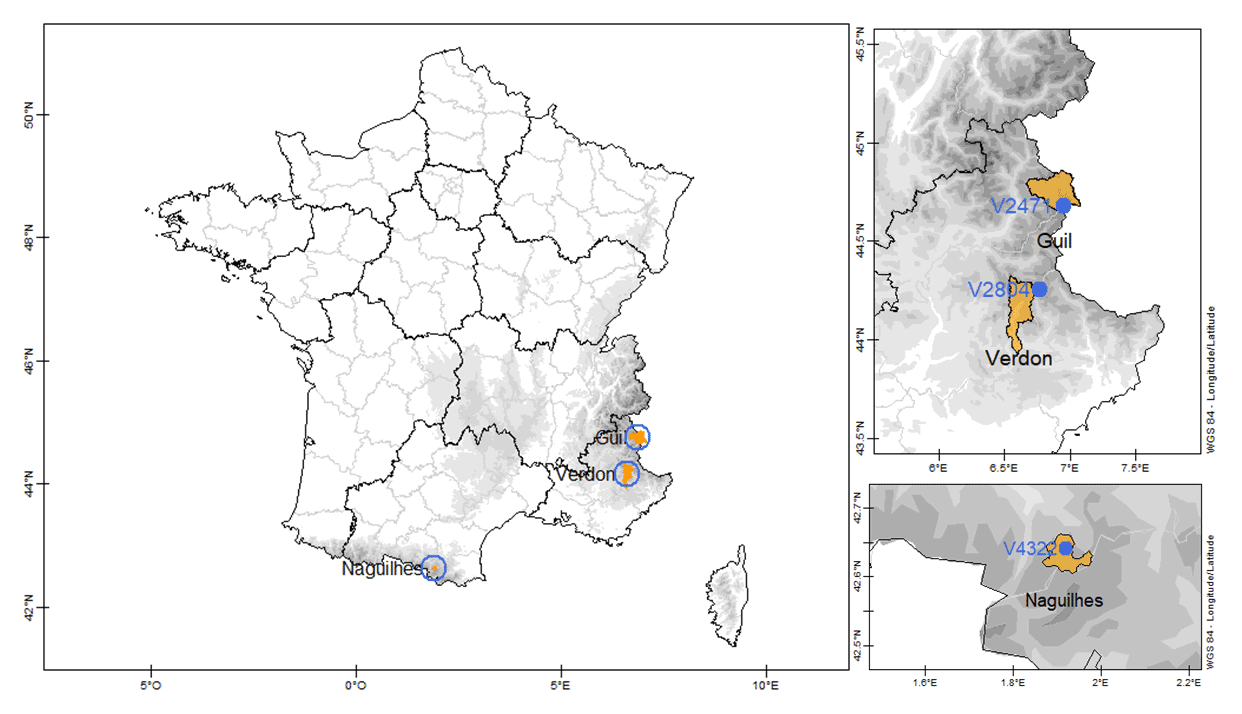
Figure 2 Geographic locations of the Verdon basin, the Guil basin in the Alps mountain range and the Naguilhes basin in the Pyrenees mountain range (left panel). In the right panels, two zooms show the locations of the in situ CRS observations: V2471, V2804 and V4322 within the Guil, Verdon and Naguilhes basins, respectively.

2.2 Hydrological basins and observations

The present study focuses on three mountainous basins: the Verdon at La Mure basin, the Naguilhes basin and the Guil at Chapelue basin (Fig. 2) that are part of the EDF hydroelectricity network. These three basins were selected according to two criteria: (i) the quality of the hydrometric data (to avoid assimilating poor-quality data); (ii) the presence of CRS data on the basin. They also offer a variety of hydroclimatic dynamics.

The Verdon at La Mure basin is a subbasin of the Durance basin located in the southern French Alps. The Verdon basin covers 404 km² and has an elevation ranging from 972 to 2990 m. The Naguilhes basin is located on a tributary of the Ariege River in the eastern part of the French Pyrenees. It is the smallest of the studied basins, covering 30 km² and with an elevation ranging from 1880 to 2750 m. The basin corresponds to the inflow from the Naguilhes hydroelectric dam. The Guil basin is a tributary of the Durance River, located in the French Alps (Hautes-Alpes). The Guil at Chapelue basin covers 418 km² and has an elevation ranging from 1313 m to 3274 m. The outlet is located just upstream from Maison du Roy dam.

Three types of observations are available in the basins: the streamflow, the CRS and the FSC.

The streamflow is the observed water flow at the basin outlet (m s⁻¹). It is a direct and reliable observation of the model state variable Q. The streamflow data have been collected by EDF almost continuously since 1997 in the Verdon basin, 1962 in the Naguilhes basin and 2004 in the Guil basin.

The CRS (Kodama et al., 1979; Paquet and Laval, 2006) is a cosmic ray snow sensor located in every basin as part of the EDF snow network and provides the SWE that informs on the state of the snow stock at a specific geographical point (see Fig. 2, right panels).

• In the Verdon basin, the instrument is located at the Sanguignères station (V2804) at an altitude of 2050 m. The CRS data are available discontinuously from 2002 to 2017.

• In the Naguilhes basin, the instrument is located at the Les Songes station (V4322) at an altitude of 2030 m. The CRS data are available discontinuously from 2004 to 2017.

• In the Guil basin, the instrument is located at the Les Marrous station (V2471) at an altitude of 2730 m. The CRS data are available discontinuously from 2005 to 2016.

The CRS measurement technique is known to provide accurate SWE estimations, except for very shallow snow depth due to instrumental limitations. It provides a very local observation (typical footprint about 5 m), which suffers from representativeness limitations. In Sect. 4.3, a detailed discussion is held on how the CRS observations are integrated in the assimilation process.

The FSC is provided by the MODIS satellite observations (Hall et al., 2006). The FSC is quantified at 500 m and daily resolutions by a value ranging from 0 to 1 for zero to full coverage. FSC data suffer from well-known limitations concerning cloud–snow discrimination and measure on complex vegetation/topography terrain. In our experiments, the FSC data are averaged on catchment scale and are available discontinuously (depending on cloud cover) from 2001 to 2015 in the Verdon basin, from 2003 to 2015 in the Naguilhes basin and from 2002 to 2015 in the Guil basin.

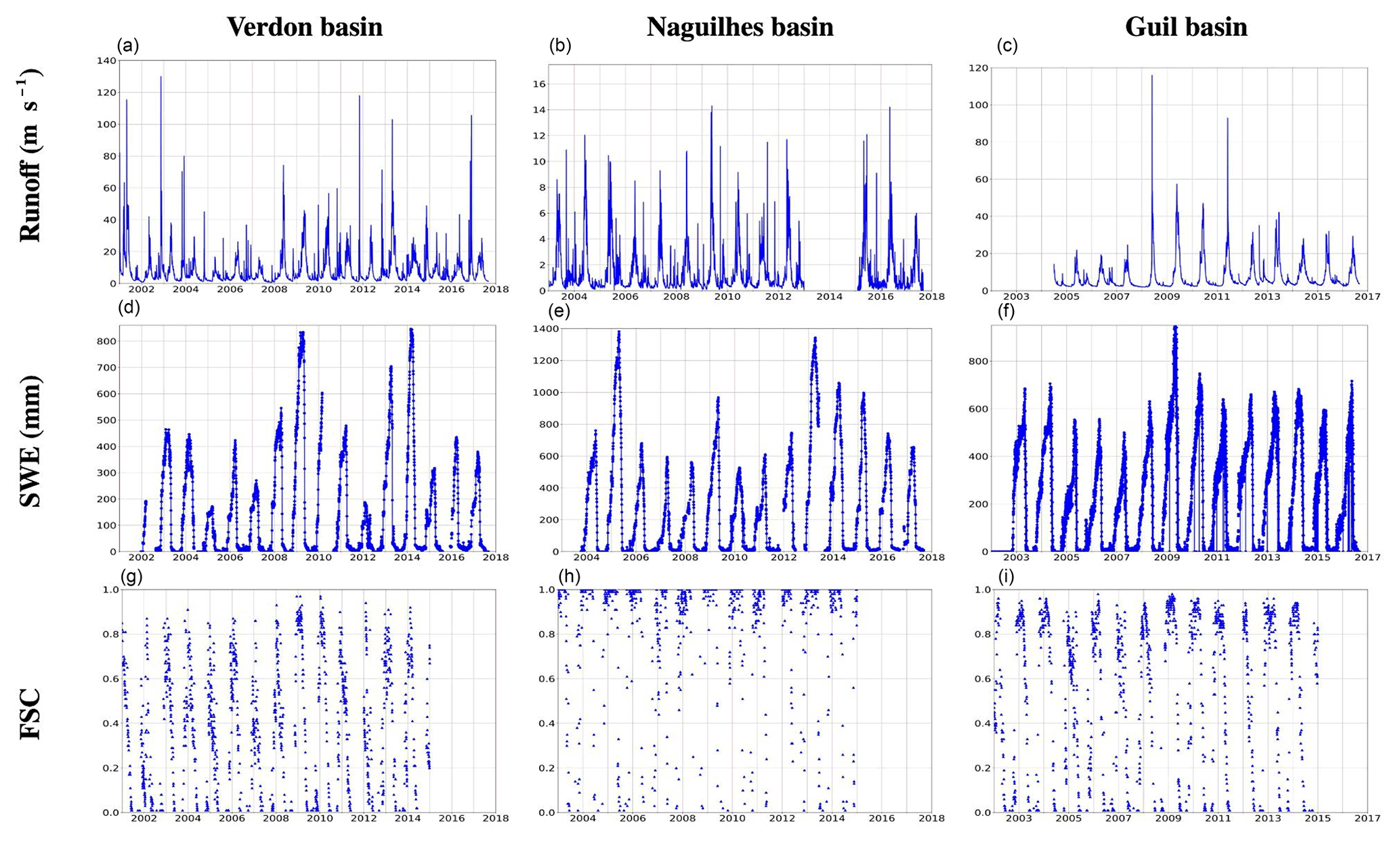
Figure 3 Available observation time series in the Verdon basin (a, d, g), in the Naguilhes basin (b, e, h) and in the Guil basin (c, f, i) of streamflow Q (a–c), CRS SWE observation (d–f) and FSC (g–i).

For all observation types, the uncertainty is difficult to quantify. This is all the more difficult for the assimilation perspective since representativeness uncertainties must be accounted for. Those are impossible to quantify with the available model and observations and may be larger than instrumental uncertainties. For these reasons, the levels of uncertainties (error variances) have been empirically tuned in the data assimilation system to avoid significant data rejection, which occurs when observation uncertainties are underestimated.

The three types of observations are displayed for each basin in Fig. 3.

The performance of the model is good in the three basins of interest, with Nash–Sutcliffe efficiencies equal to 0.846, 0.760 and 0.926, respectively, for the Verdon, Naguilhes and Guil basins over the calibration periods (1998–2013, 1987–2012 and 2004–2013, respectively).

3 Sensitivity experiment

3.1 Sobol indices

In order to better understand the sensitivity, and thus the controllability, of the MORDOR-SD model, we seek to determine which variables generate the most uncertainty in the streamflow estimate at the basin outlet. To do so, we perform a sensitivity study of the system based on the Sobol indices (Sobol', 1990; Nossent et al., 2011).

The Sobol indices evaluate the sensitivity of an output variable to an input variable. If a model links one or more random variables X_i, $i\in [\mathrm{1},n]$ (input variables) to one random variable Y (output variable), the Sobol index (of first order) of the variable X_i is based on a variance decomposition and is defined by

$$\begin{array}{}\text{(1)}& S_i={\displaystyle \frac{\mathrm{Var}\left[E\left[Y|X_i\right]\right]}{\mathrm{Var}\left[Y\right]}}.\end{array}$$

3.2 MORDOR-SD sensitivity

In the case of the MORDOR model, one can see the SSS value as an output variable and all other state variables of the model as input variables. It is then possible to run a set of ensemble simulations by perturbing each variable independently to compute Var[E[Y|X_i]] and another set by perturbing all the variables at once to compute Var[Y]. This gives the SSS sensitivity to each state variable in the model.

Figure 4 Sobol indices (%) in the Verdon configuration between the years 1968 and 2018 for a 10 % perturbation on each variable. The Sobol indices show the sensitivity of the SSS value to the variables surface storage (U), hillslope storage (L), capillarity storage (Z), snow stocks (S) and snowpack temperature (TST) at the eight altitude levels (number 1 is the lowest altitude). The last column, Av, gives the average over the entire time period. The darkest squares indicate a stronger sensitivity of the SSS to uncertainties in the snow stocks between altitude levels 5 and 7.

It should be noted that the Sobol equations make the assumption that the variables X_i are independent of each other. This is clearly not the case for the MORDOR variables; however, the goal of this experiment is not to attribute the causality of the uncertainties in Y but to assess the potential controllability of the model by each variable. In other words, if we were to control and reduce the uncertainties in X_i, with observations for instance, the Sobol indices could tell us how effective the uncertainty reduction in Y would be.

To carry out this sensitivity study, a set of simulations is generated in each basin on 1 April of each year, and the impact on the seasonal streamflow supply on 31 August is evaluated. Figures 4–6 show the Sobol indices (%) in the Verdon, Naguilhes and Guil basins, respectively, for a perturbation on each variable of 10% of its initial value (1 April). The figures show the Sobol indices between 1968 and 2018, and the last column, Av, is the average over the entire time period. The Sobol indices show the sensitivity of the SSS value to the five state variables: U, L, Z, S and TST at the eight, four and eight altitude levels in Figs. 4–6, respectively. The darkest squares indicate a stronger sensitivity of the SSS to uncertainties in the corresponding variables. The U, L and Z storages are expected to have a short-term impact on the runoff at the basin outlet, and hence uncertainties in these storages on 1 April should impact the SSS uncertainty less. This is indeed confirmed by the small Sobol indices they generate on the SSS. Uncertainty in the temperature of the snowpack TST on 1 April also seems to not have much impact on the SSS uncertainty. However, it can be seen that for all years the variable uncertainties that lead to the largest uncertainties in cumulative streamflow are the uncertainties in snow stocks at the altitude bands from S₄ to S₇ in the Verdon basin, from S₂ to S₄ in the Naguilhes basin and from S₄ to S₇ in the Guil basin. The differences between elevation bands are mainly due to the differences in their absolute snow content. For example, the high-elevation bands have smaller areas (by definition of the elevation bands), and hence they have less snow content, which leads to less uncertainty. Similarly, differences between years are most likely due to differences in snowfall since the perturbations are prescribed relative to the state variables (10 %), but the sensitivity of the streamflow is absolute.

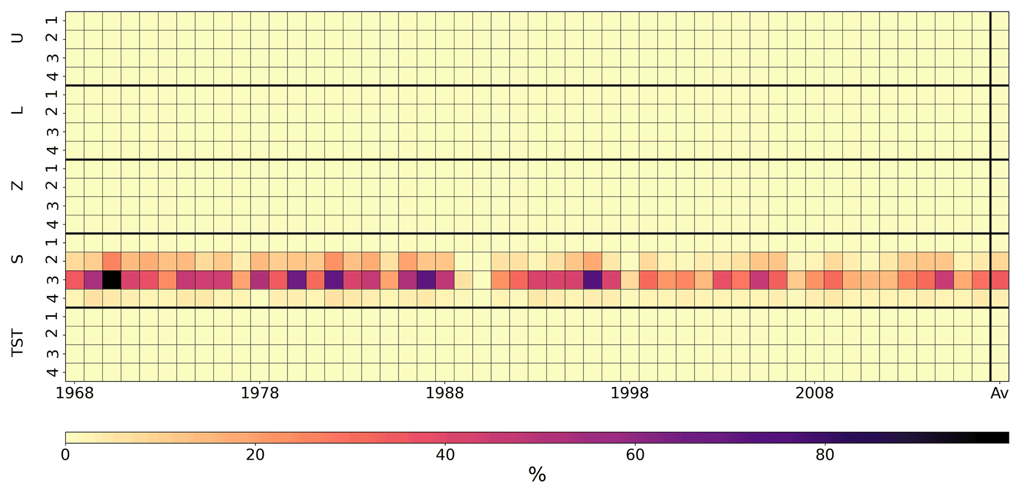
Figure 5 Sobol indices (%) in the Naguilhes configuration between the years 1968 and 2018 for a 10 % perturbation on each variable. The Sobol indices show the sensitivity of the SSS value to the variables U, L, Z, S and TST at the four altitude levels (number 1 is the lowest altitude). The last column, Av, gives the average over the entire time period. The darkest squares indicate a stronger sensitivity of the SSS to uncertainties in the snow stocks at altitude levels 2 and 3.

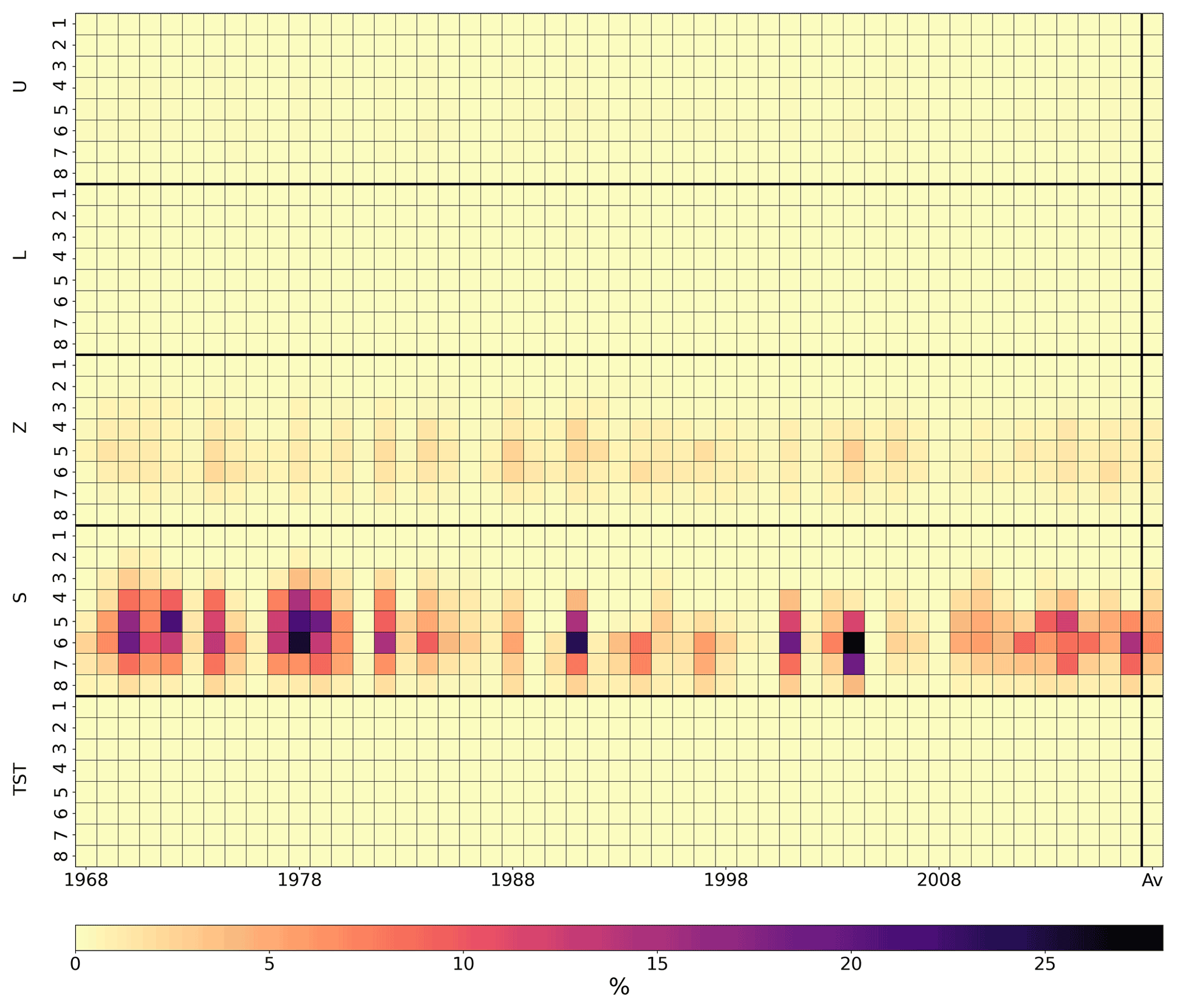
Figure 6 Sobol indices (%) in the Guil configuration between the years 1968 and 2018 for a 10 % perturbation on each variable. The Sobol indices show the sensitivity of the SSS value to the variables U, L, Z, S and TST at the eight altitude levels (number 1 is the lowest altitude). The last column, Av, gives the average over the entire time period. The darkest squares indicate a stronger sensitivity of the SSS to uncertainties in the snow stocks between altitude levels 4 and 7.

A substantial difference in sensitivity between the three basins should be noted. The Verdon basin shows a maximum of 36 % sensitivity, the Naguilhes basin 99 % and the Guil basin 28 %. This could imply that, in the Naguilhes basin, for instance, introducing accurate information on the snow stocks might have a very positive impact on the SSS estimation. On the other hand, in the other two basins, a control of the snow stocks could improve the SSS estimation but maybe to a lesser extent. This sensitivity study confirms nonetheless that controlling the snow stocks at the end of winter seems to be the most important lever to improve the SSS prediction.

4 Experimental protocol

4.1 Protocol and diagnostics

The experiments are performed during the years when CRS and streamflow observations are available: from 2002 to 2017 in the Verdon basin, from 2004 to 2017 in the Naguilhes basin and from 2005 to 2016 in the Guil basin. Every year, data assimilation is performed between 1 September and 31 March; this period is called the reanalysis period. The assimilated ensemble is then forecasted freely from 1 April to 31 August; this period is called the forecast period. The streamflow estimations are diagnosed during both the reanalysis and the forecast period. The SSS estimation, i.e., the cumulated streamflow during the forecast period, is also diagnosed.

The diagnostics performed are the continuous-rank probability score skill (CRPSS; see Hersbach, 2000, for details on the CRPS and Piazzi et al., 2018, for details on the CRPSS) according to the formulation described by Bontron (2004), with a thinness component (FinS) and a correctness component (JustS). A score of 1 represents a perfect ensemble and lower than 0 an ensemble less accurate than the climatology of the system. The FinS score can be seen as a measurement of the dispersion of the ensemble and the JustS score as the distance between the median of the ensemble and the observations. A second diagnostic is used to assess the SSS estimation: the root-mean-square error (RMSE). The RMSE is the Euclidian distance between the ensemble mean SSS estimation and the observed SSS and is computed (hm³). A perfect RMSE score is equal to 0.

4.2 Meteorological forcing perturbations

The free ensemble simulations and the assimilation ensemble simulations are generated using perturbations with AR1 processes on the forcings. The AR1 autocorrelation parameters are prescribed for all experiments as 0.9 for temperature and 0 for precipitation. Note that the AR1 process applied to precipitation is multiplicative and the one applied to temperature is additive. The AR1 standard deviations for the free ensemble were tuned to provide the most accurate SSS prediction. Figure 7 shows the CRPSS on the SSS estimation for free ensembles with several sets of AR1 standard deviation parameters (σ_P, σ_T) applied to the forcings (P, T).

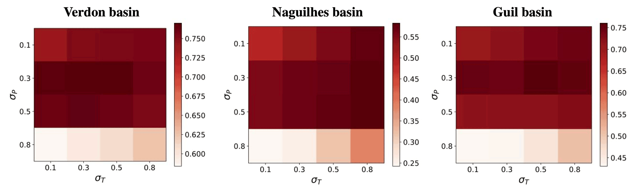
Figure 7 CRPSS of free ensemble simulations computed for AR1 parameter calibration (σ_P, σ_T). The maximum CRPSS occurs at the Verdon basin for (0.3, 0.3), at the Naguilhes basin for (0.3, 0.8) and at the Guil basin for (0.3, 0.5).

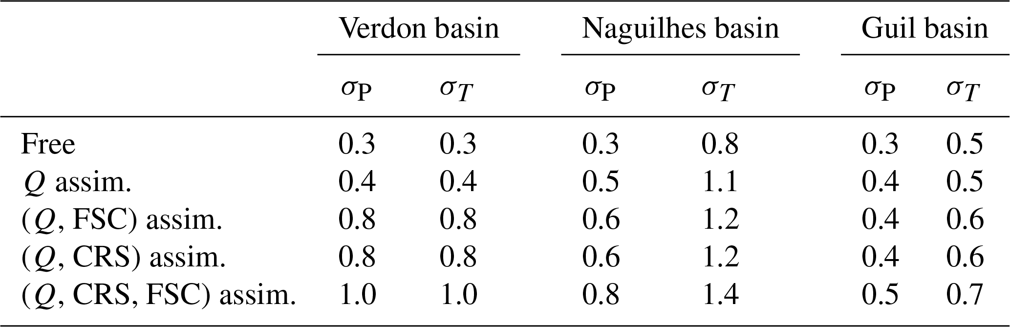
A reproducibility issue was encountered during the assimilation experiments (several experiments with the same parameters produced different results), probably due to the high nonlinearities of the system and the finite number of ensemble members. To avoid this problem, the standard deviations σ_P and σ_T of the AR1 processes on the forcings used for the assimilation were increased to stabilize the results during the reanalysis period. Then, during the forecast period, the assimilation ensemble uses the same AR1 process parameters as the free ensemble. Table 1 summarizes the AR1 parameters used in the experiments.

Table 1 AR1 process parameters applied to precipitation (ϕ_P, σ_P) and temperature (ϕ_T, σ_T) forcings for the free ensemble and the assimilation (assim.) ensembles during the reanalysis period (September to March) and the forecast period (April to August).

4.3 Assimilation setup

The assimilation is performed using a PF with sequential importance resampling (Gordon et al., 1993; Van Leeuwen, 2009). The PF determines sequentially, within an ensemble of simulations (also called particles or members), the simulations with a model state close to the observations. The PF describes the prior probability density of the system state as a Dirac sum of equal weights $\mathrm{1}/N$ for N the size of the ensemble. Using Bayes' theorem, the analysis assigns larger weights to the simulations closer to the observations. The weights are then used to resample the simulations farthest from the observations so that the simulations closest to the observations are duplicated. In this study, we use a stratified resampling method introduced by Kitagawa (1996). The duplicated simulations are not perturbed after resampling. The dispersion of the ensemble is maintained only by the perturbations on the forcings. Several studies showed the need for additional perturbation after resampling in order to avoid ensemble collapse, yet this does not seem necessary in our system.

The free ensemble and the assimilation ensemble are composed of 900 members. The PF provides the exact Bayes theorem solution for an infinitely large ensemble but quickly suffers from the curse of dimensionality (Snyder et al., 2008) and underperforms with small ensemble sizes. Some experiments have been performed with smaller ensembles (not shown here) and confirm this issue. Due to the very nonlinear nature of the hydrological model, the assimilation performances were not necessarily poor but unstable, meaning that they would fluctuate when repeated. Since the goal of the present paper is not to suggest the most appropriate assimilation method for operational use but is rather to assess whether information on the SSS exists and can be retrieved from snow stock observations, we have chosen to use a very large ensemble.

The assimilation window for all the experiments is a 3 d window; i.e., an analysis is performed every 3 d using the last three daily observations.

4.4 Observation operators

In order to allow small time lags between simulated and observed streamflow, the three streamflow observations in the 3 d assimilation window are averaged to make a single observation. Streamflow observation error variance is then prescribed as a function of the observed streamflow Q_obs (similarly to Clark et al., 2008, Weerts and El Serafy, 2006, and Piazzi et al., 2021):

$$\begin{array}{}\text{(2)}& {\mathit{\sigma }}_Q^{\mathrm{2}}=\mathit{\alpha }\cdot Q_{\mathrm{obs}}^{\mathrm{2}},\end{array}$$

with α=0.3. Also, a minimal threshold of ${\mathit{\sigma }}_Q^{\mathrm{2}}=\mathrm{0.2}$ is used so as to avoid unreasonably low uncertainties for very small streamflow.

The assimilation is performed using the FSC-normalized anomalies. The anomalies are computed by subtracting the daily FSC climatologic average from the daily FSC value of the current year, and this difference is then divided by the climatologic average. The anomaly indicates with a positive or negative value whether the snow cover is especially high or low this year on that day. The same is done to the fractional snow cover computed by the model. The observation error variances of the FSC-normalized anomalies are prescribed at σ_FSC=0.3.

Finally, as previously mentioned, CRS observations are local data and do not necessarily represent the snow dynamics of an entire basin. Hence, the first step of the CRS observation operator is to consider the CRS-normalized anomalies, similarly to the FSC observations. However, after several tests (not shown here), the CRS-normalized anomaly does not provide the correction needed for the model snow stock anomaly at the appropriate altitude band. A second step of the CRS observation operator was then to systematically compare, at each assimilation window, the CRS anomaly to the forecasted model snowpack anomaly at all altitude bands. The closest (in terms of CRPSS) altitude band is then considered to be the observed band. This can be seen as an adaptive observation operator. This process does slightly impact the computation time (as it has to be performed every 3 d in this case) but significantly improves the results in our study. The observation error variances of the CRS anomalies are prescribed at σ_CRS=0.3.

5 Assimilation results

5.1 Streamflow reanalysis for September to March

During the September to March period, the observations are available daily. In this subsection, only streamflow observations are assimilated. As an illustration, Fig. 8 shows the time series of Q during the year 2002 in the Verdon basin. The reanalysis period corresponds to the times left of the vertical dotted black line and the forecast period to the times right of that line. While panels a and b highlight the high confidence of the assimilated ensemble (red lines) versus the free ensemble (green lines) with a reduction in dispersion, panel c shows that the median after assimilation (red line) is more accurate than the median without assimilation (green line) with respect to the observations (blue line).

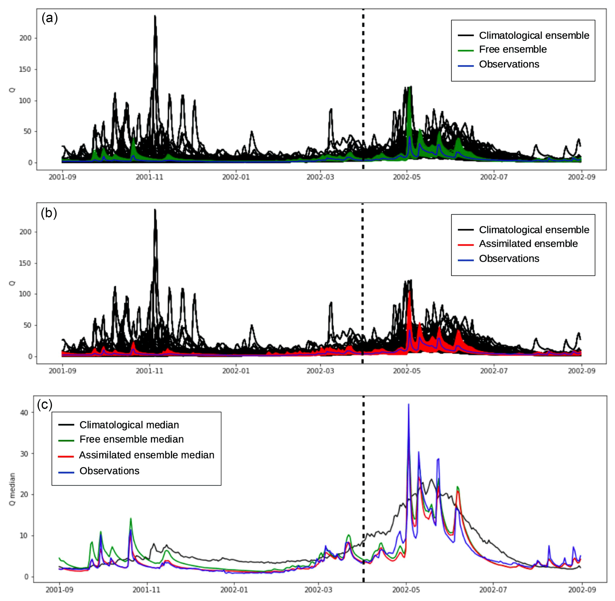
Figure 8 Streamflow time series Q, during the year 2002 for the Verdon basin, of the observed streamflow (blue), the climatological ensemble (black), the free ensemble (panel a; green) and the assimilated ensemble (panel b; red) for the assimilation of Q. Panel (c) represents the ensemble's respective medians. The vertical dotted black line represents the separation between the reanalysis period (before the line) and the forecast period (after the line).

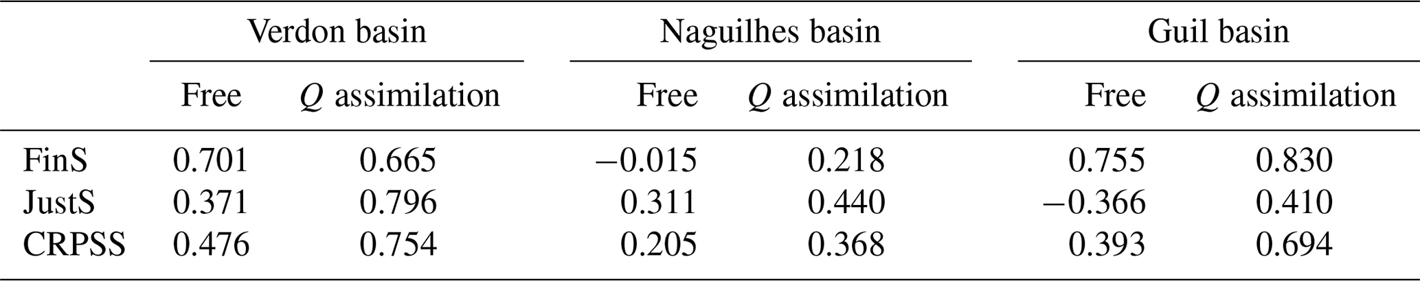
The first conclusions drawn from the year 2002 are confirmed over the 16 years 2002–2017 in the Verdon basin, the 12 available years between 2004 and 2017 in the Naguilhes basin and the 10 available years between 2005 and 2016 in the Guil basin, with the use of the probabilistic score CRPSS and its components FinS and JustS summarized in Table 2. The FinS of the free ensemble is higher than the FinS of the assimilated ensemble, which is not abnormal since the ensembles have not been generated with the same perturbations and the assimilated ensemble perturbations were much stronger. However, the assimilation increases the JustS of the free ensemble from 37.1 % to 79.6 % in the Verdon basin, 31.1 % to 44 % in the Naguilhes basin and −36.6 % to 41 % in the Guil basin. This results in a CRPSS of 75.4 %, 36.8 % and 69.4 % after assimilation when the free ensemble CRPSS was 47.6 %, 20.5 % and 39.3 % in the three basins, respectively.

Table 2 Probabilistic scores on streamflow Q during the reanalysis period, from September to March, for the free ensemble (“Free”) and the streamflow assimilation (Q assimilation).

Assimilation of streamflow observations combined with CRS and FSC observations has been compared to streamflow-only assimilation and has very little to no impact on the results during this reanalysis period (not shown here). This is due to the very straightforward task of constraining simulated streamflows using the accurately observed streamflow. Indeed, the PF sequentially selects and resamples the simulations with a streamflow closer to the observations.

An interesting specificity of the particle filter, as a data assimilation method, is that, each time, not only are the accurate streamflows selected, but also all the corresponding state variables. In other words, one can hope that the assimilation will have also selected more accurate snow stocks, which will then help produce better streamflow predictions during the following spring and summer seasons.

5.2 Streamflow forecast for April to August

Figure 9 shows the streamflow time series of the ensemble medians (climatologic ensemble in black, free ensemble in green and assimilated ensemble in red) and the observed streamflow (in blue) during the year 2011 in the Verdon basin for the Q assimilation (panel a) and the (Q, CRS) assimilation (panel b). The streamflow assimilation (Fig. 9a) seems to improve the short-term (first 5 to 10 d) streamflow forecast. However, the streamflow forecast is then overestimated after a couple of weeks, but a good control of the snowpack with (Q, CRS) assimilation (Fig. 9b) reduces this long-term streamflow forecast overestimation. Hence, the overall streamflow forecast remains improved in the first few weeks of the forecast period in comparison to the free ensemble, and the overestimation during the rest of the forecast period is avoided.

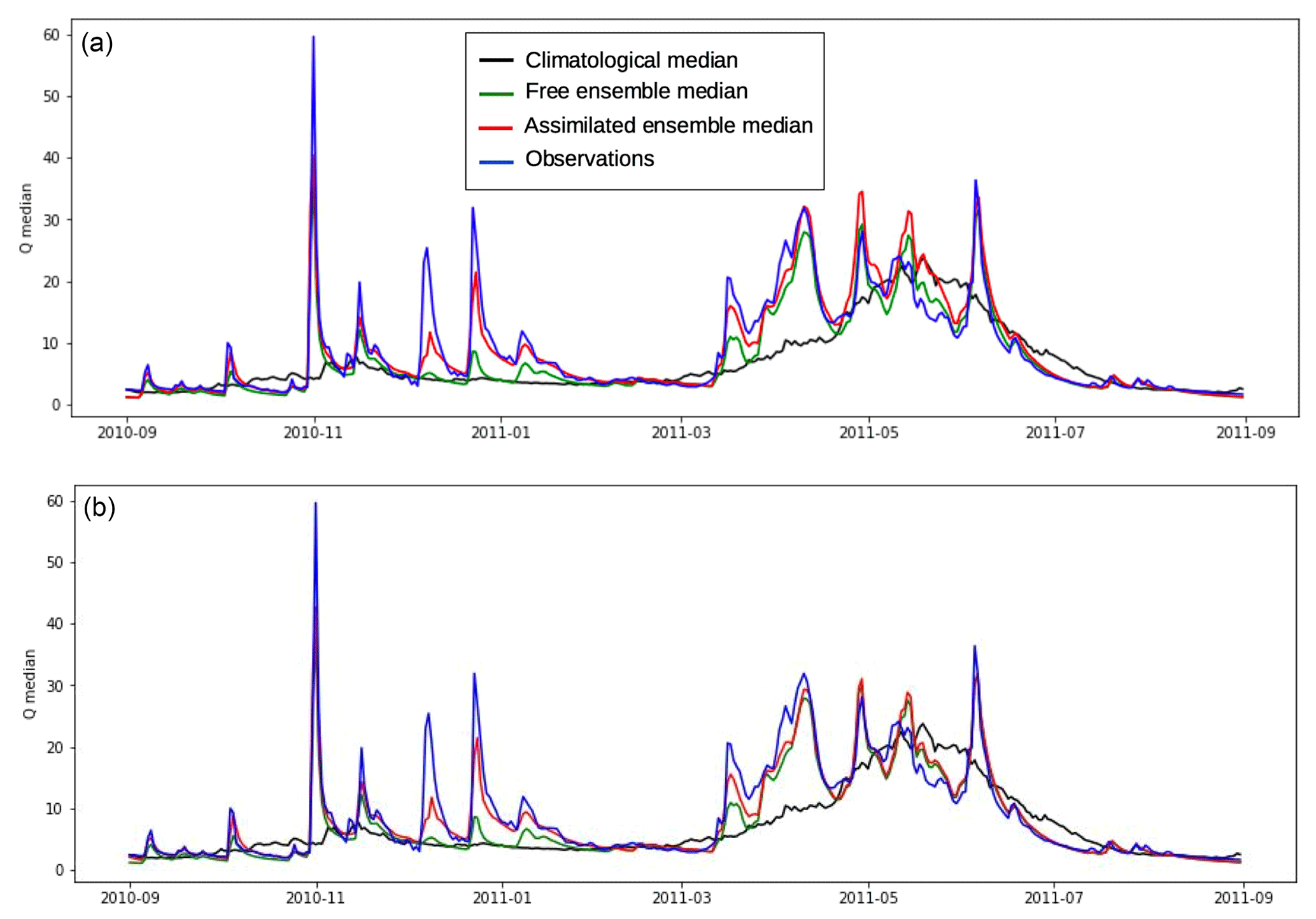
Figure 9 Same as Fig. 8c, during the year 2011 in the Verdon basin, for the Q assimilation (a) and the (Q, CRS) assimilation (b).

This result is confirmed by the CRPSS for all years available and in two of the three basins: the Verdon and Naguilhes basins (Fig. 10). Both (Q, CRS) and (Q, FSC) assimilations show a CRPSS increase in comparison to Q-only assimilation. In the Naguilhes basin, in particular, the streamflow assimilation improvement over the “Free” ensemble (approximately from a CRPSS of 0.44 to 0.455) is almost doubled by the additional use of CRS (approximately to a CRPSS of 0.465). This significant improvement in the Naguilhes basin could be due to the strong sensitivity of the streamflow to the snow stock uncertainty as implied by the Sobol experiment conclusions (Sect. 3).

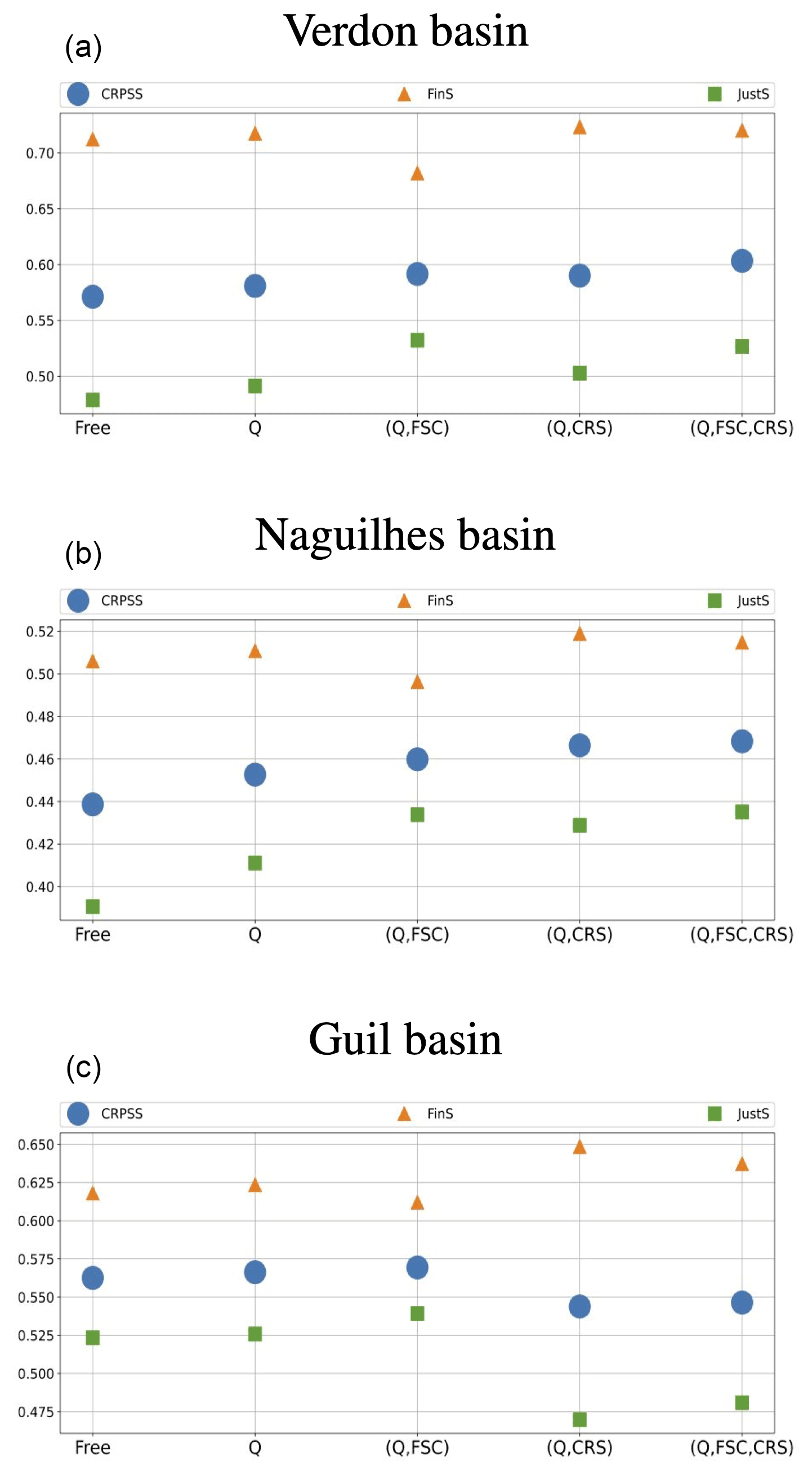
Figure 10 Probabilistic scores in the Verdon basin (a), Naguilhes basin (b) and Guil basin (c) for the forecasted streamflow Q by the free ensemble (“Free”) and the four assimilation experiments.

In the Guil basin, the streamflow forecast is degraded by the use of CRS data. This overall result is in fact due to some years in particular where the CRS information contradicts the observed streamflow. The case of the Guil basin will be further discussed in the following section.

In general, the improvement brought by an accurately controlled snowpack to the streamflow estimation is slim in terms of scores. The variation in the CRPSS is almost always smaller than 5 %. This is due to the fact that, even though the snow stock might be improved, the timing of the streamflow runoff is mainly driven by the anticipated meteorological forcings during the forecast period. The cumulated streamflow, or seasonal streamflow supply, however should be less impacted by the timing of the runoff and should be significantly improved by a better-estimated snow stock.

5.3 SSS forecast

Global scores have been computed to assess the abilities of the different assimilation configurations to estimate the SSS, i.e., the cumulated runoff between April and August. Similarly, Figs. 10 and 11 show the global CRPSS, FinS and JustS of the SSS ensemble estimations in the three basins, and Fig. 12 shows the RMSE of the ensemble means.

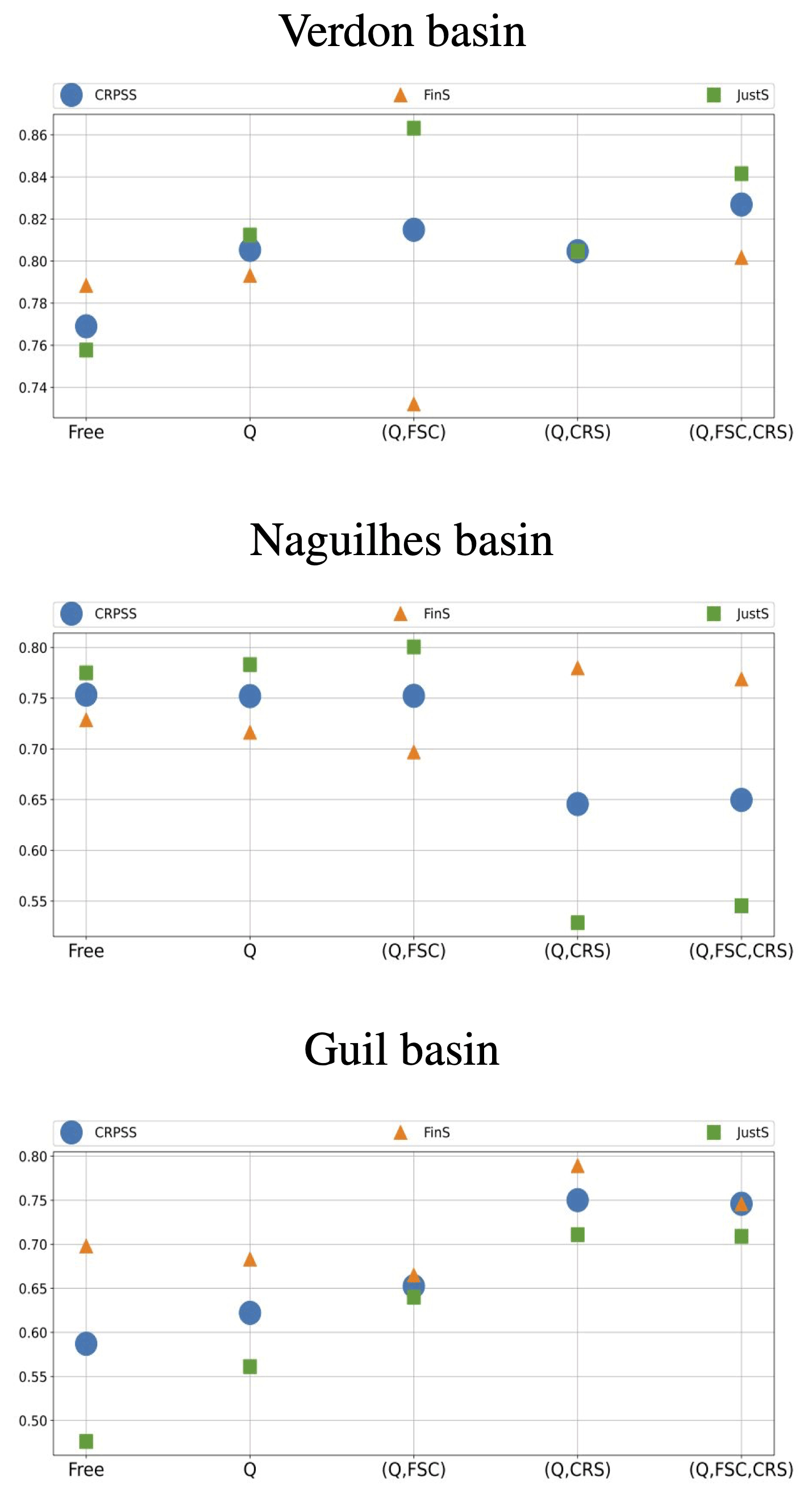
Figure 11 Probabilistic scores for the forecasted SSS by the free ensemble (Free) and the four assimilation experiments.

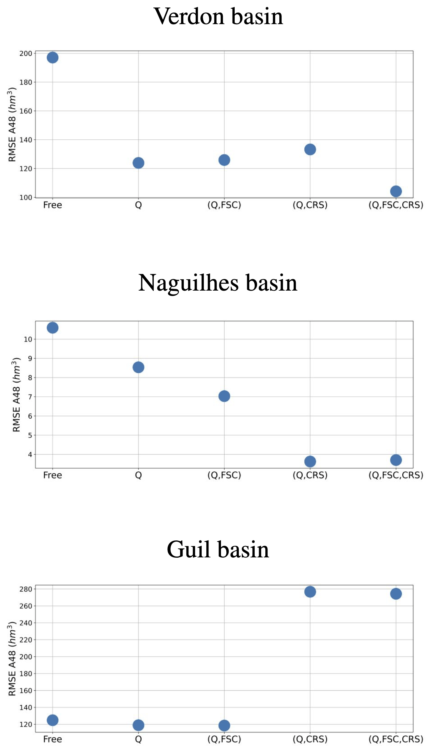
Figure 12 RMSE for the forecasted SSS by the free ensemble (Free) and the four assimilation experiments. Not shown here, the climatology RMSEs are 3603.43 hm³ in the Verdon basin, 57.26 hm³ in the Naguilhes basin and 2079.76 hm³ in the Guil basin.

As for the streamflow estimation, the SSS estimation is improved by assimilating all the available data in the Verdon basin and the Naguilhes basin. In the Verdon basin, the Q assimilation increases the CRPSS from 77 % (free ensemble) to 80.5 %, and the (Q, FSC, CRS) assimilation further increases the CRPSS to 82.7 %. Meanwhile, the RMSE of the free ensemble SSS mean (200 hm³) is almost halved by the (Q, FSC, CRS) assimilation and reduced to a little over 100 hm³. In the Naguilhes basin, the Q assimilation increases the CRPSS from 58.7 % (free ensemble) to 62.2 %, the (Q, CRS) assimilation further increases the CRPSS to 75 % and the (Q, FSC, CRS) assimilation CRPSS is slightly lower at 74.6 %. The RMSE is strongly reduced by the use of CRS observations. Both the (Q, CRS) and (Q, FSC, CRS) assimilations reduce the free ensemble SSS mean RMSE, which is over 10 hm³, to under 4 hm³. Once again, these very good performances in the Naguilhes basin are likely due to the significant sensitivity of the SSS estimation to the snow stock uncertainty that was highlighted by the Sobol sensitivity experiment (Sect. 3).

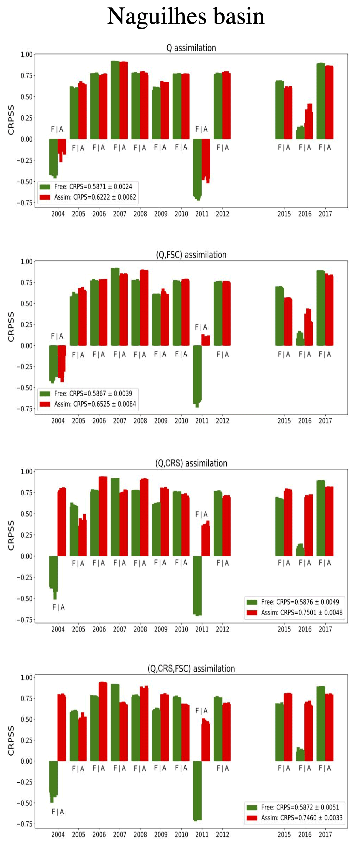
The yearly SSS CRPSS histograms presented in Figs. 13 and 14 allow us to understand how combining all the observations improves the global scores. Every year, the free ensemble SSS CRPSS (green) is compared to the SSS CRPSS of the assimilated ensemble (red) for the different assimilation configurations. As a reminder, a negative CRPSS indicates that the ensemble estimation is less accurate (in terms of CRPS) than the climatological ensemble. In the Verdon basin, the main inaccurate free ensemble SSS estimation occurs in 2014. During that year, only the assimilation configurations containing CRS observations are able to truly correct that estimation. Meanwhile, in 2003 for instance, the (Q, CRS) assimilation deteriorates the SSS estimation. However, only assimilating (Q, CRS, FSC) manages to improve both 2003 and 2014. Similarly, in the Naguilhes basin, the years 2004 and 2011 are poorly estimated by the free ensemble, the Q assimilation and the (Q, FSC) assimilation, but both the (Q, CRS) and (Q, FSC, CRS) assimilations significantly increase the SSS CRPSS. These yearly variations show that the hydrological problem considered here is not a linear and Gaussian problem where adding observations systematically improves the estimation every year. These variations can be due to the quality or representativity of those observations, which can also vary from one year to the next. However, in this case, the benefits of combining multivariate data come from the particle filter-selection process, which behaves as a data cross-validation of sorts that will take advantage of the most appropriate observations each year. This remains true, however, as long as none of the observations is widely inaccurate.

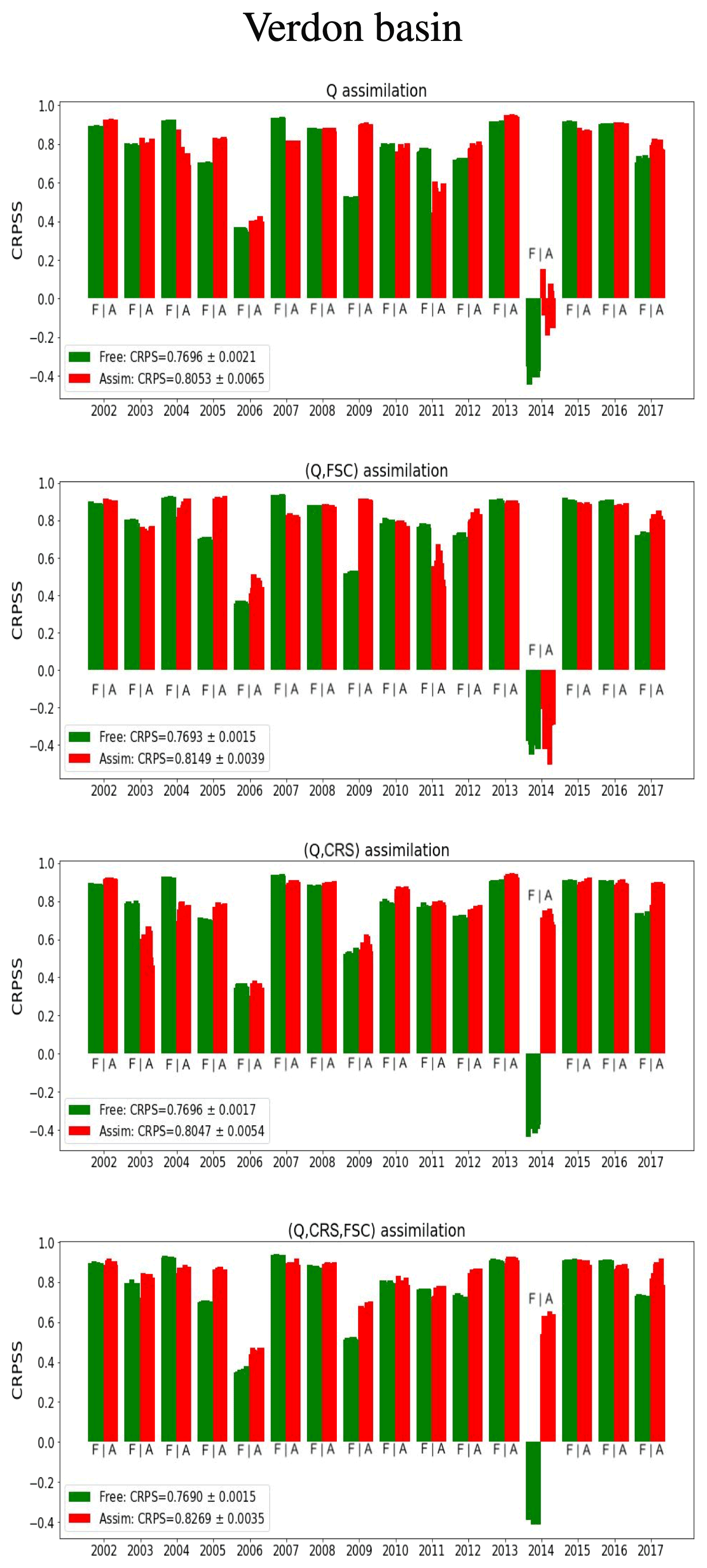
Figure 13 Yearly CRPSS of the SSS for the free ensemble (green) and the assimilated ensemble (red) from the Q assimilation, (Q, FSC) assimilation, (Q, CRS) assimilation and (Q, CRS, FSC) assimilation (10 experiments each year) in the Verdon basin.

Figure 14 Same as Fig. 13 in the Naguilhes basin.

Figure 15 Same as Fig. 13 in the Guil basin.

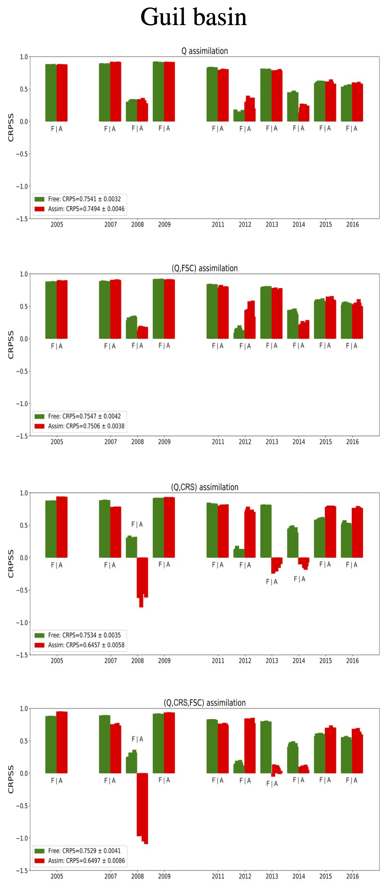
For instance, in the Guil basin, the detrimental impact of the CRS observations is even larger on the SSS estimation than it is on the streamflow estimation. The average CRPSS declines from approximately 75 % to 65 % (Fig. 10), and the RMSE increases from 120 to 280 hm³ (Fig. 11). Similarly to Figs. 13 and 14, the yearly histograms in Fig. 15 reveal that the assimilation performances differ significantly from one year to the next. In particular, the histograms reveal that the SSS estimation in 2012 is improved by the CRS observations. However, for the years 2008, 2013 and 2014, the CRS observations seem to completely mislead the SSS estimation. This behavior can be explained by (1) the particularly wide area covered by the Guil basin and (2) specific atmospheric events during those years, both rendering the CRS observations unrepresentative of the hydrological situation of the basin. In particular, for the year 2008, the poor results can be explained both by the non-representativity of the CRS observations and by a historical flooding episode at the end of May associated with strong uncertainties in precipitation.

6 Summary and conclusions

The objective of this work is to assess the potential of using local snow observations such as cosmic ray sensor (CRS) observations and fractional snow cover (FSC) data in order to improve the estimation of the seasonal streamflow supply at the outlet of a mountainous basin. The assimilation of streamflow measurements is commonly performed and is known to improve the short-term prediction of hydrological system evolution. However, combining different snowpack observations at basin scale, such as FSC data, and at local scale, such as CRS data, could improve the prediction of seasonal streamflow supply between April and August (SSS).

As a first step, a sensitivity test performed in Sect. 3 shows that snow stock control has the potential to strongly reduce the uncertainties in the SSS. The Sobol indices (relative variances) demonstrate a significant sensitivity of the SSS to uncertainties in the snow stocks at different altitudes (S₄ to S₈ in the Verdon basin, S₂ to S₄ in the Naguilhes basin and S₄ to S₇ in the Guil basin). Although expected, this result supports the idea that assimilating data containing snow stock information can improve SSS estimation.

The streamflow assimilation is confirmed to be beneficial for the streamflow estimation during the reanalysis period from September to March (Sect. 5.1), the streamflow prediction (after the assimilation) from April to August (Sect. 5.2) and for the SSS estimation (Sect. 5.3). Indeed, in the three basins, the Q assimilation significantly improves the streamflow estimation during the reanalysis period: from 47.6 % to 75.4 % in the Verdon basin, from 20.5 % to 36.8 % in the Naguilhes basin and from 39.3 % to 69.4 % in the Guil basin. Also, the streamflow forecast during the 5-month forecast period is systematically improved by the Q assimilation, albeit slightly. Finally, the SSS CRPSS of the Q assimilation is increased compared to the one of the free ensemble for both the Verdon and Naguilhes basins and remains approximately constant in the Guil basin. In all the basins, the SSS RMSE of the Q assimilation ensemble mean is smaller than the free ensemble mean.

Since the streamflow assimilation seems to be improving the SSS estimation, further experiments were performed in Sect. 5.2 to assess the combination of streamflow and other observations. Also, separate tests were performed to assess CRS-only and FSC-only assimilations in the hydrological system (not shown here), but not using the streamflow observations seemed to strongly deteriorate the SSS estimation. Section 5.2 shows that, in two of the three basins, the combination of FSC and CRS with Q in the assimilation process has proven to be very beneficial to the SSS estimation. In the Verdon and Naguilhes basins, where it was identified that FSC and CRS are beneficial, the best strategy seems to be that all available observations are to be included in the assimilation process, so that if in some years one observation type misrepresents the hydrological situation, the others can counteract its effect. For instance, in the Verdon basin, the (Q, FSC) assimilation degrades the estimation in 2014, and in 2003 the (Q, CRS) assimilation degrades the estimation, but when assimilating (Q, CRS, FSC), both those years are improved. The overall scores show that the (Q, FSC, CRS) assimilation when compared to the Q-only assimilation increases the SSS estimation CRPSS by 2 % in the Verdon basin and by 22 % in the Naguilhes basin and reduces the SSS estimation RMSE by 19.7 hm³ in the Verdon basin, corresponding to a 15.9 % improvement, and by 4.8 hm³ in the Naguilhes basin, corresponding to a 56.6 % improvement.

Caution should be applied with this strategy since, in the Guil basin during specific years, the CRS observations can largely misrepresent the hydrological situation, thus significantly deteriorating the streamflow and SSS estimations. More specifically, during three years (2008, 2013 and 2014) the CRS observations appear to contradict the streamflow observations, hence misleading the SSS estimation. This can be explained by specific atmospheric events occurring during those years and leading to highly heterogeneous precipitation patterns.

The present study showed that assimilating multivariate data in a basin-scale hydrological model is possible and can improve long-term predictions such as the SSS estimation. In two of the three basins, the assimilation of snow observations has proven to be beneficial, improving the overall performances. This result was achieved by incorporating local CRS data into a basin model through the use of an adaptive observation operator on the elevation band. While heuristic, the adaptive observation operator has proven to be successful in most cases. However, in some years, the poor representativity of local CRS observations can degrade the performance of the data assimilation process. Combining the sources of observations therefore appears to be the best guarantee of robustness for operational purposes. Also, the multivariate assimilation allowed us to highlight that the CRS observations in one of the studied basins and during specific years are not appropriate for assimilation and should be disregarded.

As a continuation of this work and to keep improving SSS prediction in operational forecasting systems, several other aspects must be investigated further. First, a wider study should be conducted using the same experimental setup to assess the benefits and issues of the available observations, in particular the CRS data, in a larger panel of hydrological basins. Options to compensate for the lack of representativity of the CRS data in some basins are limited. A study on the cost and benefit to densify the observation network in the concerned basins should be conducted by operational centers. A more attractive, because less expensive, alternative could be to better characterize and/or improve the representativity of SWE data at the basin scale by using the existing large network of snow poles that may contain complementary SWE information. Finally, moving from the semi-distributed MORDOR model to the fully spatialized MORDOR model (Rouhier et al., 2017) should make the integration of local CRS information into the physics of a basin model more realistic and ultimately improve the SSS estimation.