Canopy structure, topography, and weather are equally important drivers of small-scale snow cover dynamics in sub-alpine forests

In mountain regions, forests that overlap with seasonal snow mostly reside in complex terrain. Due to persisting major observational challenges in these environments, the combined impact of forest structure and topography on seasonal snow cover dynamics is still poorly understood. Recent advances in forest snow process representation and increasing availability of detailed canopy structure datasets, however, now allow for hyper-resolution (<5 m) snow model simulations capable of resolving tree-scale processes. These can shed light on the complex process interactions that govern forest snow dynamics. We present multi-year simulations at 2 m resolution obtained with FSM2, a mass- and energy-balance-based forest snow model specifically developed and validated for metre-scale applications. We simulate an ∼3 km² model domain encompassing forested slopes of a sub-alpine valley in the eastern Swiss Alps and six snow seasons. Simulations thus span a wide range of canopy structures, terrain characteristics, and meteorological conditions. We analyse spatial and temporal variations in forest snow energy balance partitioning, aiming to quantify and understand the contribution of individual energy exchange processes at different locations and times. Our results suggest that snow cover evolution is equally affected by canopy structure, terrain characteristics, and meteorological conditions. We show that the interaction of these three factors can lead to snow accumulation and ablation patterns that vary between years. We further identify higher snow distribution variability and complexity in slopes that receive solar radiation early in winter. Our process-level insights corroborate and complement existing empirical findings that are largely based on snow distribution datasets only. Hyper-resolution simulations as presented here thus help to better understand how snowpacks and ecohydrological regimes in sub-alpine regions may evolve due to forest disturbances and a warming climate. They could further support the development of process-based sub-grid forest snow cover parameterizations or tiling approaches for coarse-resolution modelling applications.

1 Introduction

The presence of snow in the sub-alpine forest ecoregion of the European Alps, and other mountain ranges across the Northern Hemisphere, means large areas of seasonal snow cover overlap with both forests and complex topography. Snow accumulation and ablation processes are known to be controlled by the structure of the forest cover (Mazzotti et al., 2019a), topographic characteristics (Broxton et al., 2020; Safa et al., 2021; Schirmer and Pomeroy, 2020) as well as how these physiographic factors interact with local climate and weather patterns (Lundquist et al., 2013; Seyednasrollah and Kumar, 2019; Pflug and Lundquist, 2020). Consequently, snow cover dynamics in sub-alpine forests are subject to strong complexity and variability down to small spatial and temporal scales. A thorough understanding of the controlling factors is important, because snow cover dynamics affect ecohydrological regimes (e.g. Barnhart et al., 2016; Manning et al., 2022), microclimate and habitat characteristics (e.g. Niittynen et al., 2020), and land surface energy exchange (e.g. Webster and Jonas, 2018; Manninen and Jääskeläinen, 2018). Today, snow cover regimes are changing due to climate warming (Mote et al., 2018; Marty et al., 2017; Notarnicola, 2020; Bormann et al., 2018), and forest structure is being altered by man-made and natural disturbances (Bebi et al., 2017; Seidl et al., 2017; Goeking and Tarboton, 2020). In view of these changes, understanding forest-snow dynamics can inform adequate management strategies – particularly in regions where downstream water supply is dependent on snow resources from forested headwaters (Sturm et al., 2017; Siirila-Woodburn et al., 2021). However, it remains unclear if and how the response of snow cover dynamics to environmental change will depend on where this snow is located within the heterogeneous landscape.

Canopy structural controls on individual forest processes have been widely addressed in both experimental and modelling studies. Interception of snow by the canopy (Moeser et al., 2015; Roth and Nolin, 2019), transmission of shortwave radiation, and enhancement of longwave radiation (Malle et al., 2019; Mazzotti et al., 2019b; Webster et al., 2016; Lawler and Link, 2011), have received particular attention due to the strong spatial variability of these processes induced by tree-scale canopy structural heterogeneity. Existing research has, however, focused on flat sites to single out the effect of canopy structure. Only few studies have considered how the combination of forest and topography alter accumulation and ablation processes under forests relative to clearings. Ellis et al. (2011) presented measurements from a Canadian site, including short- and longwave irradiances and snow depth under the canopy and in clearings on different slopes and aspects, and they showed that the presence of forest delayed snowmelt relative to open areas more strongly on south-exposed slopes than on north-exposed ones. In a modelling study, Strasser et al. (2011) found that forest cover diminished aspect-dependent differences in snow cover dynamics compared to openings, and they further noted that forest effects differed between years with varying meteorological conditions. Neither of these studies did, however, consider fine-scale canopy structure in detail, and no study that specifically addresses inter-annual consistency of fine-scale forest snow distribution patterns exists to our knowledge.

In recent years, the increased availability of lidar-derived snow depth distribution datasets has enabled a new approach to analysing forest snow cover dynamics. Multiple studies have attempted to establish relationships between snow, canopy, and terrain descriptors based on such datasets (Zheng et al., 2019; Mazzotti et al., 2019a; Currier and Lundquist, 2018). Broxton et al. (2020) used maps of snow water equivalent (SWE) and time series of snow depth transect measurements to analyse the combined impact of forest density and topographic location on snow water equivalent in a semi-arid climate. Safa et al. (2021) applied machine learning to identify the factors that determine snow disappearance in different forest and topographic settings based on snow depth maps covering four US sites with variable climate characteristics. Recently, Koutantou et al. (2022) presented a time series of uncrewed aerial vehicle (UAV) lidar datasets to compare the evolution of snow depth distribution patterns on opposed slopes in an Alpine valley. All these studies were limited to process inferences as snow distribution datasets only reflect the combined impact of various forest snow processes.

Instead of relying on snow data alone, understanding process interactions can be advanced through sophisticated process-based models. In the absence of observational data or for predictive purposes, models are commonly used as a best estimate of reality (Wood et al., 2011; Wrzesien et al., 2022). In forest snow research, the use of hyper-resolution models that resolve tree-scale processes is gaining popularity in applications that require the small-scale variability of these processes to be adequately represented (Harpold et al., 2020). To our knowledge, two models developed specifically for this purpose exist to date: SnowPALM – Snow Physics and Lidar Mapping (Broxton et al., 2015) and FSM2 – Flexible Snow Model (Mazzotti et al., 2020a, b). They evolved independent of each other but follow similar principles: at every modelled location, the computation of forest snow processes considers the specific canopy structure both directly overhead and in the surroundings of the location of interest. This approach acknowledges the fact that different characteristics of the canopy are relevant for different processes. For instance, it allows for a model grid cell located in a forest gap to be unaffected by interception of snow in the canopy (due to lack of overhead canopy) but still experience reduced insolation and wind speeds (due to sheltering by the surrounding canopy), whereas a grid cell underneath a tree at the canopy edge may be affected by both interception and direct insolation. Such a representation requires explicit canopy structure descriptors to be derived from canopy structure data at equally high spatial resolution.

The benefit of hyper-resolution canopy representations relative to traditional approaches that rely on bulk canopy descriptors like leaf area index (LAI) and average canopy height only has been demonstrated for both FSM2 and SnowPALM. Both models have been shown to effectively capture detailed snow depth distribution patterns when compared to manual and lidar-derived measurements (Broxton et al., 2015; Mazzotti et al., 2020b). In addition, FSM2 has also been validated at the level of individual processes by comparing modelled sub-canopy incoming short- and longwave radiation, air and snow surface temperature, and wind speed, against spatially and temporally resolved observational datasets (Mazzotti et al., 2020a). To our knowledge, such a validation approach is unprecedented, revealing remarkable improvements in resolving canopy-mediated processes at a high spatial and temporal resolutions.

Their ability to accurately capture process variability has made hyper-resolution forest snow models attractive research tools. Impact studies have used SnowPALM to analyse the effect of forest disturbance on snow water resources under varying meteorological conditions (Moeser et al., 2020) and to assess forest thinning strategies (Krogh et al., 2020). Hyper-resolution models also provide an approximation of processes that are not resolved in coarser-resolution models and can thus inform the development of sub-grid parameterizations of these processes. As such, both SnowPALM (Broxton et al., 2021) and FSM2 (Mazzotti et al., 2021) have been used to derive recommendations for modelling forest snow processes at coarser resolutions, and there is still great potential to further exploit these models for scientific purposes.

In this study, we used hyper-resolution modelling to explore the spatio-temporal dynamics of individual forest snow processes and their effect on snow cover evolution in forested complex terrain under varying meteorological conditions. We applied FSM2 to a sub-alpine valley and across multiple winters to assess the interplay of canopy structure, topography, and meteorology. Our work builds on Koutantou et al. (2022), who observed considerable differences in snow distribution dynamics between their sites located on south- and north-exposed forested slopes over the course of one snow season. The authors hypothesized that weaker correlations between snow depth and canopy cover at the south-exposed slope than at the north-exposed slope were due to differences in the shortwave irradiance regimes at the two locations but could not fully demonstrate this based on their observational data of snow depth alone. The modelling approach used here allowed us to overcome the limitations of their study by leveraging the capabilities of FSM2 to accurately represent both snow distribution and the spatio-temporal dynamics of the underlying processes. Based on the respective simulations, we analysed individual processes and their interactions over larger spatial and temporal extents than previously possible, where equivalent observational datasets are inexistent. Our goals were (1) to characterize spatial patterns of snow cover dynamics and the underlying processes in such a sub-alpine environment, (2) to detect connectivity between snow patterns and patterns of underlying processes, and (3) to assess their temporal consistency throughout the season and between different years. By contributing to the improved understanding of these dynamics, we hope to facilitate the development of approaches to treat sub-grid variability in coarser-resolution models and to help expand our capabilities to assess the impact of environmental change on ecohydrological processes.

2 Methods

2.1 Study area

We focused our modelling in a domain situated in the Flüela valley near Davos (Fig. 1) in the eastern Swiss Alps. The climate is inner-alpine with an average wintertime (DJF) air temperature of $-\mathrm{4.2}{}^{\circ }$C and 450 mm yearly snowfall sum (Davos station, MeteoSwiss, norm period 1991–2020; http://www.meteoschweiz.ch, last access: 24 May 2023). The model domain is contained in a 2.5 × 1.5 km area at the entry of the valley, which consists of two opposite (south- and a north-facing) slopes. Both slopes extend over 500 m elevation span from the valley bottom at 1570 m a.s.l. to the treeline around 2100 m. Maps of the topographic characteristics of the model domain (elevation, slope, and aspect) are included in the Supplement (Fig. S1.1).

Figure 1 Overview of the study area: (a) Location of the model domain within Switzerland and on the topographic map of the Davos area (source: swisstopo), including locations of the automatic weather stations DAV and WFJ; (b) Canopy height model and contour lines (equidistance: 50 m), including locations of the sites from Koutantou et al. (2022) and of the sub-domain shown in Figs. 5 and 7–9.

The forest comprises needleleaf species, predominantly Norway spruce (evergreen) with some individual larches (deciduous), which is typical of this sub-alpine forest ecoregion. Understorey vegetation is short, mainly consisting of blueberry bushes and grasses. Trees range from new to old growths with maximum heights of 35 m, and forest structure includes both dense stands and gaps of varied sizes. The domain thus spans a range of variability in canopy structure and topographic conditions over a rather small area, which is common in the sub-alpine environment.

The site is at ∼5 km distance to well-established and predominantly flat research sites that have hosted recent experimental forest snow process studies from the WSL Institute for Snow and Avalanche Research (SLF), including Laret (Malle et al., 2019; Webster et al., 2017), Seehornwald (Webster et al., 2016), and Ischlag (Moeser et al., 2015). The sites from Koutantou et al. (2022) are fully contained in the perimeter of this study. Operational measurements from the automatic weather station (AWS) Davos (DAV) and from the measurement field at Weissfluhjoch (WFJ) are within 1 and 3 km of the site, respectively (Fig. 1a).

2.2 Modelling framework

Snow cover simulations with the Flexible Snow Model FSM2 (Mazzotti et al., 2020b, a) are at the core of this study's methodology (Fig. 2). FSM2 is the upgrade of the physics-based, medium-complexity Factorial Snow Model, FSM (Essery, 2015), with forest canopy added. It includes all major canopy processes (interception of snow in the canopy, subsequent unloading and sublimation, shortwave radiation transfer, longwave radiation enhancement, and wind attenuation) with well-established parameterizations. We applied the version presented by Mazzotti et al. (2020a) specifically developed for hyper-resolution (metre-scale) simulations, FSM2.0.3 (Mazzotti et al., 2020c). This version uses process-specific canopy metrics, computed for each modelled location. Notably, insolation through the three-dimensional forest canopy is explicitly represented by importing time series of transmissivity for direct shortwave radiation from an external radiative transfer model. This allows for achieving the accuracy of very detailed, ray-tracing-type radiative transfer modelling approaches without compromising the complexity and computational efficiency of FSM2. For this study, we ran FSM2 at 2 m grid spacing (i.e. 850 000 points) and hourly resolution for six winters (i.e. water years (WY) 2016–2021). Our model application follows Mazzotti et al. (2021), who used equivalent hyper-resolution simulations to explore model upscaling behaviour.

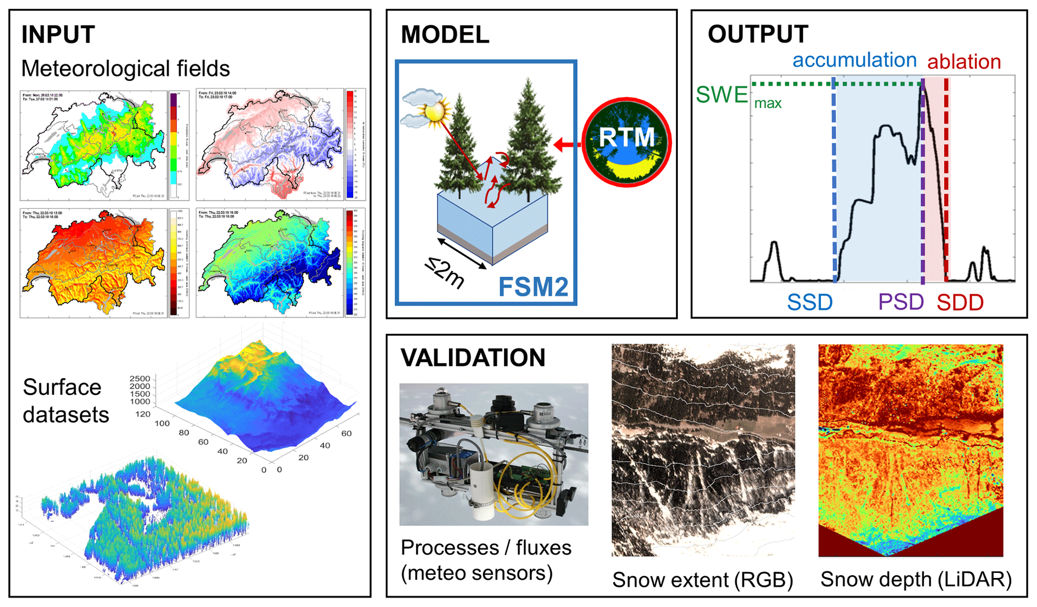
Figure 2 Conceptual sketch of the study methodology. Input meteorological and surface datasets (from the OSHD and the 2017 lidar mission, Sect. 2.2), FSM2 including external radiative transfer model, evaluation approaches (presented in Mazzotti et al. 2020a and Sect. 2.3) and resulting snow cover dynamics descriptors: peak SWE (SWEmax), start of snow cover period (SSD), day of peak SWE (PSD) snow disappearance date (SDD) – see Sect. 2.4 for definitions.

Lidar datasets acquired through airborne laser scanning (ALS) in 2017 in the context of the first European mission of the Airborne Snow Observatory (ASO; Painter et al., 2016; Mazzotti et al., 2019a) provided the basis for computing all canopy metrics required by FSM2.0.3, including vertically projected canopy cover, canopy height, canopy density (i.e. LAI), and sky-view fraction in the full hemispherical view; for details, see Mazzotti et al. (2021, 2020b) and the Supplement S2. Shortwave transmissivity time series at each location were obtained with the workflow from Webster et al. (2020), which calculates transmissivity through an overlay of a hemispherical image and solar position at any given point in time, as presented by Jonas et al. (2020). In Webster et al. (2020), lidar-derived synthetic hemispherical images based on a methodology originally proposed by Moeser et al. (2014) were used for this purpose. Through point-cloud-enhancing techniques, the resulting images capture the shape and fine-scale structure of every individual tree in the surrounding, enabling highly accurate calculations of subcanopy radiation (Fig. S3.2). The workflow was calibrated using real hemispherical images at our sites and using the same lidar data (Koutantou et al., 2022), allowing direct application also in this study. Additional surface datasets (e.g. elevation) were available through SLF's Operational Snow-Hydrological Service's (OSHD) modelling framework. These data were provided at 25 m resolution and interpolated to the model resolution (2 m).

Meteorological forcing was also available through OSHD. As described by Griessinger et al. (2019), gridded data of all necessary meteorological input variables (incoming short- and longwave radiation, air temperature and relative humidity, wind speed, rain- and snowfall rates, and atmospheric pressure) were provided by MeteoSwiss (COSMO-1 product) at hourly interval and 1 km resolution over all of Switzerland and further downscaled to model resolution. Additional corrections (for biases or terrain effects) were applied to some of the variables, e.g. wind speed (Winstral et al., 2017) and shortwave radiation (Jonas et al., 2020). We refer to Griessinger et al. (2019) for details. By leveraging OSHD methods, this study benefitted from the currently best meteorological forcing datasets available for the site, exploiting latest downscaling approaches specifically developed for snow modelling in complex terrain. Here, input fields were initially downscaled to 25 m and subsequently linearly interpolated to 2 m resolution.

2.3 Validation of model use case

FSM2's capability to accurately simulate sub-canopy snow energetics and to thus reproduce realistic small-scale forest snow cover dynamics has been demonstrated in a dedicated study (Mazzotti et al., 2020a). Their detailed model validation was done in the vicinity of our study area, with the same type of input data and for the same type of canopy data. A summary of the validation approach and results is provided in the Supplement S3. For this reason, another model validation is beyond the scope of this study; nevertheless, an assessment of our simulations against available snow distribution datasets was performed to ensure plausibility of the model application for our use case. We considered four independent data sources: (1) daily snow depth data from stake readings acquired next to automatic weather stations (AWS) in Davos and Weissfluhjoch to assess the simulations at open sites; (2) high- and medium-resolution satellite RGB imagery available through Planet Explorer (http://www.planet.com, last access: 31 January 2022) at approx. weekly intervals for the last 5 modelled WY's, including Landsat 8, Sentinel-2, and PlanetScope, to evaluate modelled snow cover extent during periods of partial snow cover; (3) maps of sub-canopy snow depth over the full domain from two of the 2017 ASO lidar acquisitions (see Sect. 2.2) at 3 m spatial resolution, parts of which were used by Mazzotti et al. (2019a); and (4) time series of sub-canopy snow depth maps over two 150 m × 150 m domains (see Fig. 1) on the two opposed slopes obtained with UAV-borne lidar in 2020, presented by Koutantou et al. (2022). For details on the lidar campaigns, the reader is referred to the corresponding publications.

Figure 3 presents examples of visual comparisons of model simulations to satellite (Fig. 3a–b), ALS (Fig. 3c–d), and UAV-lidar data (Fig. 3e–f). These assessments reveal that the model captures the general characteristics of snow depth and snow disappearance patterns well. The strong temporal lag in snow disappearance between the south- and the north-facing slope is clearly visible in the satellite imagery and likewise reproduced by the FSM2 simulations. Snow distribution features such as preferential ablation along south-exposed forest edges and higher snow amounts in canopy gaps compared to nearby under-canopy locations in the north-exposed slope are also clearly present in both the lidar datasets and the simulations. Overall, the validation supports the evidence that FSM2 simulations are suitable for this use case. Goodness-of-fit measures would be confounded by uncertainties in meteorological input and snow measurement inaccuracies (see, for example, Raleigh et al., 2015; Günther et al., 2019; Currier et al., 2019) and were therefore not considered here.

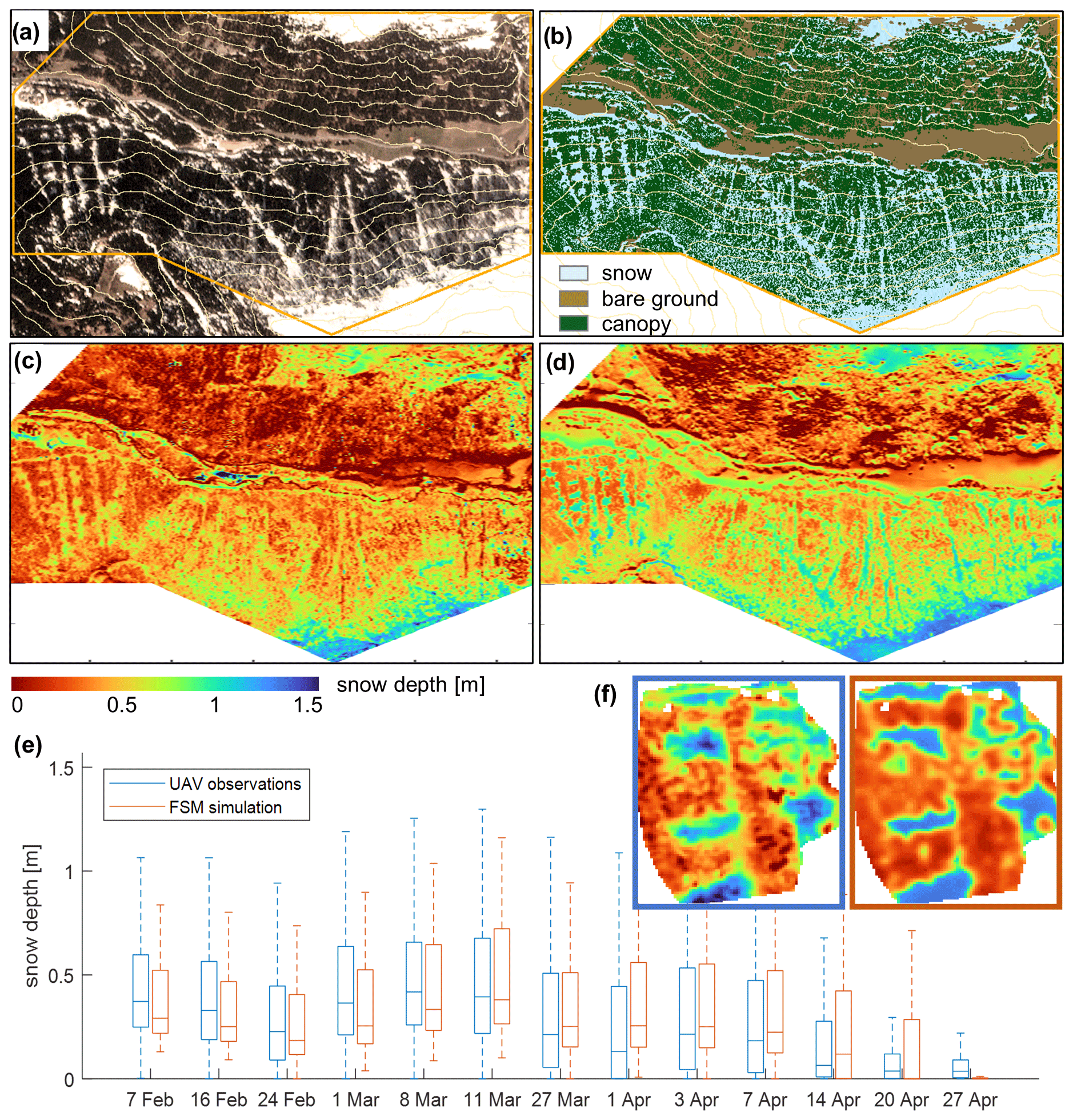
Figure 3 Examples of plausibility checks performed to verify the model use case, including comparisons of (1) satellite RGB imagery acquired by PlanetScope on 28 April 2018 (a) and snow cover extent simulated by FSM2 on the same day (b); (2) snow depth distribution derived from ALS data (c) and simulated by FSM2 (d); and (3) snow depth statistics of UAV-lidar-derived snow maps at the north-exposed site and resulting from FSM2 (e) and observed and modelled spatial distribution of the 8 March 2020 campaign (f).

2.4 Analysis approach

Our analysis uses several descriptors of the snow season and of the surface energy exchange processes derived from the FSM2 simulation results. These metrics were computed at each modelled location (i.e. 2 m grid cell) for all winters as follows.

1. Peak SWE. The maximum value of snow water equivalent on the ground attained over the course of a snow season or WY.

2. Day of peak SWE (PSD). The day on which peak SWE occurred. In the case of multiple occurrences of peak SWE over the season, the median was selected.

3. Accumulation period. Period between the last occurrence of SWE <10 mm prior to peak SWE and the day of peak SWE.

4. Start of snow cover period (SSD). The first day of the accumulation period.

5. Ablation period. Period between the day of peak SWE and the first occurrence of SWE <10 mm following peak SWE.

6. Snow disappearance day (SDD). The last day of the ablation period; also referred to as melt-out.

7. Snow cover duration. The number of days between the start of snow cover and snow disappearance.

8. Ablation rate. The quotient between peak SWE and the length of the ablation period.

9. Cumulative ablation. Amount of SWE depleted over the course of a specific time interval (computed as sum of SWE decrements including losses due to both melt and sublimation).

10. Average surface energy fluxes. Incoming and net short- and longwave radiation as well as turbulent (sensible and latent) heat fluxes into the snowpack, averaged over a specific time interval, where positive fluxes indicate transport towards the snow surface.

Note that the temporal integration varies for different metrics, with some applying to the point-specific snow cover durations and some integrating over fixed time intervals. The choice of temporal integration interval was motivated by the purpose of the corresponding analysis. Moreover, it should be noted that the definition of contiguous accumulation and ablation periods until/from peak SWE, as applied here, implies that melt events can occur during the accumulation and snowfall events during the ablation periods, respectively. The 10 mm threshold applied to define snow vs. no-snow conditions served to ensure that only days with snow present throughout the whole day would be included in the analysis of ablation rate and surface energy fluxes.

To assess relationships of any snow or process descriptor to canopy structure, we quantified the fine-scale canopy structure at a point in terms of local canopy cover fraction, one of the canopy metrics provided as input to FSM2 (“fveg”; see Mazzotti et al., 2020b). This variable describes the fraction of the vertically projected canopy cover within a 5 m radius around each modelled location, taking values between 0 and 1. We used local canopy cover fraction, because it was shown to be strongly correlated with small-scale snow depth distribution at flat sites (Mazzotti et al., 2020b) and in steep terrain (Koutantou et al., 2022).

3 Results

The following sections present a systematic analysis of FSM2 simulation results, aimed at illustrating the interplay of canopy structure, topographic, and meteorological controls. We first provide a general overview of snow cover dynamics across the site for all simulated years to provide context (Sect. 3.1) and then consider the spatial distribution of our snow descriptors in more detail (Sect. 3.2). To help interpret spatial patterns, we analyse the combined impact of the physiographic factors, topography and canopy structure, first on the temporal evolution (Sect. 3.3) and then on the spatial distribution (Sect. 3.4) of snow cover dynamics and the underlying processes. Finally, we explore the impact of meteorological conditions on the temporal consistency of said spatial patterns between water years (Sect. 3.5).

3.1 Overview of simulated snow cover dynamics

Figure 4 summarizes the statistics of the different snow season descriptors for all simulated years, aiming to give an overview of their within-year variability (attributable to variations in canopy structure and topography) and of their between-year variability (attributable to variations in driving meteorology). A summary of meteorological conditions during the simulation period is provided in the Supplement (Figs. S3.1–3.2). The start of continuous snow cover strongly varies both across the model domain and between the years (Fig. 4a). The medians within the model domain vary by 2 months, ranging from 5 November (WY 2019) to 5 January (WY 2017). Noteworthily, the spread of the start of snow cover varies strongly between the simulated WYs as well. While in 3 years snow cover onset happens basically simultaneously across the entire domain (WYs 2017, 2018, 2019), partial melt-out during snow accumulation causes heterogeneous snow cover onset dates across the domain in the other years, with interquartile ranges of full snow cover onset of over a month.

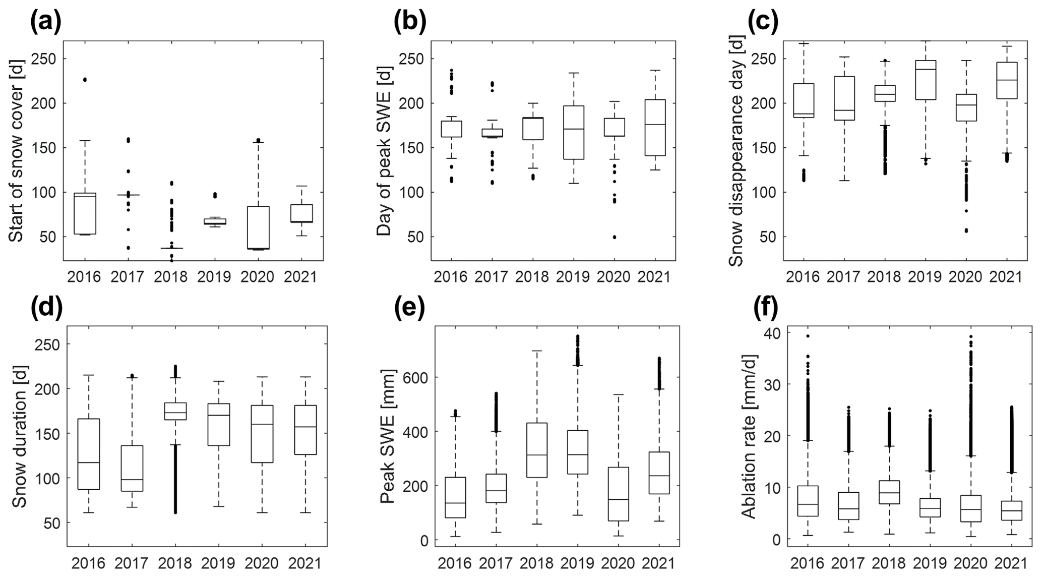
Figure 4 Summary statistics of snow season descriptors across the full model domain and for all simulated water years (WY), including (a) the start of snow cover period, (b) day of peak SWE, (c) snow disappearance day, (d) duration of full snow cover, (e) peak SWE, and (f) ablation rate. Descriptors denoting specific points in time (a–c) are indicated in terms of day since 1 October.

The timing of peak SWE (Fig. 4b) is, on average, much more consistent over the years, with median peak SWE ranging from 11 March (WY 2020) to 1 April (WY 2018). However, the spread across the model domain in each year can be large (interquartile range of approx. 2 months in WYs 2019 and 2021), which means that there can be a considerable temporal offset in the start of the ablation period across the site. Notably, this leads to some locations reaching peak SWE only when others have melted out already (overlap of boxes for day of peak SWE and snow disappearance day of the same year). The rather large spread in snow disappearance day within each year (Fig. 4c), with interquartile ranges between 2 and 6 weeks, is the result of spatial variability in both accumulation and ablation rates and is thus not surprising. Between-year variability in melt-out timing is much larger than for timing of peak SWE, with medians between 10 April (WY 2016) and 26 May (WY 2019). Further, also peak SWE itself varies (Fig. 4e), with median peak SWE across the model domain between 135 mm (WY 2016) and 314 mm (WY 2019), mostly reflecting years with higher and lower snowfall, respectively. Notably, interquartile ranges are not systematically higher or lower for higher or lower median peak SWEs occurrences.

The combination of the variable start of snow cover and snow disappearance days implies highly variable snow cover durations (Fig. 4d). Median full snow cover duration across the model domain varies between 96 (WY 2017) and 173 (2018) days, and interquartile range varies between 19 (WY 2018) and 65 (WY 2020) days. Snow cover duration can also be interpreted as the combination of amount of SWE to be depleted and efficiency of ablation processes. Notably, ablation rates (Fig. 4f) are more uniform across the WYs (median 5.5–9 mm d⁻¹) but still rather variable across the model domain (interquartile ranges of 3.6–5.9 mm d⁻¹).

It should be highlighted that there does not appear to be any clear link between any of the individual snow cover descriptors; for instance, higher peak SWE does not seem to imply longer snow duration, and later snow disappearance is not linked to higher ablation rates. Essentially, this is a consequence of accumulation and ablation processes being affected by different meteorological drivers.

3.2 Spatial patterns of snow cover dynamics

The large spread in the boxplots in many of the subpanels of Fig. 4 indicates that most snow season descriptors exhibit strong spatial variability across the model domain during most years. In Fig. 5, we present spatial maps of the same snow season descriptors for WY2019 to analyse the full spatial patterns behind this variability. To better demonstrate the spatial details, we zoom in to a sub-domain (Fig. 1) that comprises the entire range of canopy covers, elevation ranges, slopes, and aspects yet representing the physiographic character of the entire domain well. Equivalent plots over the full model domain are included in the Supplement (Figs. S5.1–5.3) for interested readers.

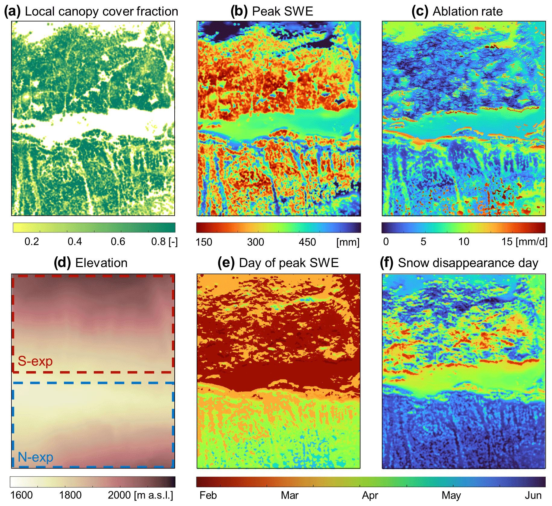
Figure 5 Canopy cover (a) and topographic (d) maps, as well as snow season descriptors including peak SWE (b), ablation rate (c), day of peak SWE (e), and snow disappearance day (f) for a sub-section of the model domain and WY 2019.

Figure 5 illustrates how peak SWE, ablation rates, day of peak SWE, and snow disappearance date vary across the landscape as a function of canopy and within the complex topography. The link between peak SWE and canopy structure (Fig. 5a vs. b) is obvious and reflects the impact of snow interception by the canopy on accumulation, which scales with local canopy cover. This dependency is well visible when comparing peak SWE at under-canopy vs. open/gap locations (Fig. 5b). Yet, a closer look at the gaps and forest edge areas (especially in the upper, south-exposed part of the domain) reveals a rather large spread in peak SWE for these locations with low to no local canopy cover, even within this relatively small sub-domain of 1.5 km². For this specific example, the spread in peak SWE amounts to approx. 200 mm. Consequently, canopy structure is clearly not the only factor controlling peak SWE distribution, despite the strong correlation between peak SWE and local canopy cover fraction with Pearson's correlation coefficient (R) ranging from −0.89 (2018) to −0.76 (2017). Note that correlation coefficients are computed over the full model domain.

When interpreting spatial patterns of peak SWE, it is important to consider that the timing of peak SWE also varies across the domain (i.e. ablation starts in some areas while others are still accumulating snow; Fig. 5e). Generally, the onset of the ablation period occurs earlier on the south-exposed slope. The earliest onsets occur along the canopy edge at lower elevations, but there is no evident simple relationship with canopy cover. The combination of strong variability in peak SWE and heterogeneous peak SWE timing means that spatial patterns of ablation rates (Fig. 5c) and snow disappearance date (Fig. 5f) are complex, with non-trivial dependencies with either canopy cover or topography (Fig. 5d).

Notably, snow disappearance day is more variable on the south-exposed slope than in the north-exposed slope, where snow disappearance is restricted to a shorter time span. Complex melt-out patterns on the south-exposed slope hint at considerable spatial heterogeneity in ablation processes which override accumulation patterns, so the spatial structure of snow disappearance is considerably different from that of peak SWE (Fig. 5b vs. f, upper part). In contrast, this is not the case on the north-exposed slope: here, under-canopy areas melt out earlier than canopy gaps, which means that melt-out patterns generally have a similar spatial distribution as accumulation patterns (Fig. 5b vs. f, lower part). These similarities suggest that on the north-exposed slope spatial variations in ablation rates are not strong enough to supersede spatial variations in accumulation. We will look at the physical processes that drive these patterns in more detail in the following sections.

Ablation rates (Fig. 5c) exhibit spatial patterns that do not correspond to any other snow season descriptor. Remarkable features are the maxima along the south-facing canopy edge on the south-exposed slope and in the canopy gaps on the higher-elevation areas of the north-exposed slope. This is where snow generally either starts to melt first or last (compare to Fig. 5e). Furthermore, large canopy gaps on both slopes generally feature higher ablation rates than adjacent under-canopy areas. Note that assessing the dependencies of ablation rate on canopy structure and topography is confounded by the necessity to calculate ablation rates over the local ablation period (see definition in Sect. 2.4), which itself varies across the domain due to variable timings of peak SWE and snow disappearance.

3.3 Impact of canopy structure and topography on the temporal evolution of the snow cover and underlying processes

The analysis in Sect. 3.2 clearly suggests that the interaction between canopy structure and topography plays a relevant role in shaping spatial snow cover dynamics. To understand these patterns and the processes that lead to them, it is instructive to consider time series of snow cover evolution at some representative locations. We manually selected seven locations that cover the existent range of canopy structures and topographic settings to showcase potential outcomes of process interactions in a systematic way. We include points located at the north- and south-facing edges of canopy gaps for both north- and south-exposed slopes, as well as three points located under canopy (two on the south- and one on the north-exposed slope; the two points on the south-exposed slope differ in their proximity to a sun-exposed canopy edge, where point 1 is more sun-exposed and point 2 more shaded). The locations of these points are marked in the Supplement (Fig. S6). Figure 6a shows SWE at these seven locations for WY 2019. Note that we will look at data from other years and the influence of weather on inter-annual differences in Sect. 3.5.

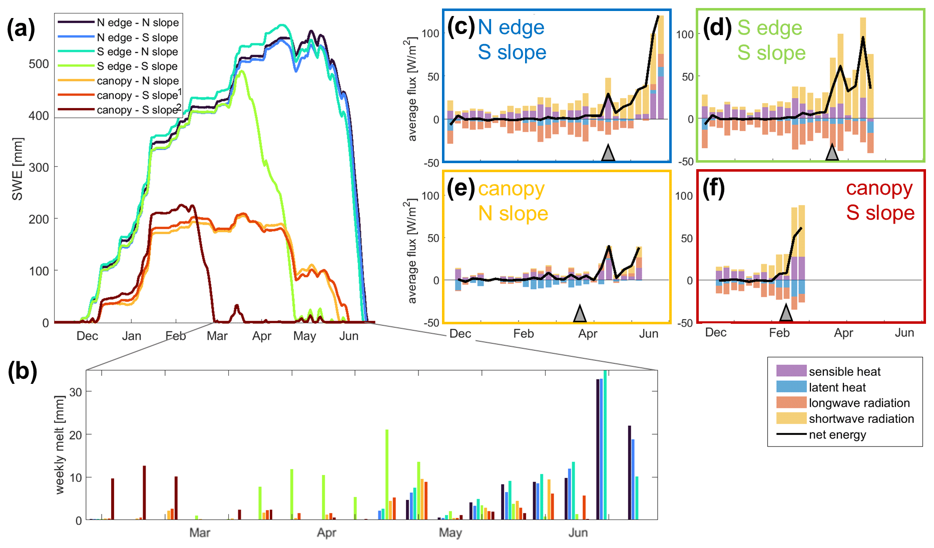
Figure 6 Interactions between canopy structure and topography illustrated at seven example points (locations see S3). Time series of SWE (a), weekly melt during the ablation period (b) and surface energy balance partitioning at four of the points (c–f). In c–f, bars show weekly average fluxes, while the black line depicts their sum, grey triangles mark the day of peak SWE, and only periods with snow on the ground are shown.

At the beginning of the accumulation period, all three points that are located under canopy accumulate less snow than all points located in gaps. These two distinct pathways reflect the fact that, if no major precipitation gradients exist across the site and if ablation processes or the impact of wind redistribution is negligible, interception of snow is the only process that introduces spatial variability during this phase. Canopy structure thus exerts the primary control on snow accumulation. However, as the season progresses, further pathways fork off. In this example, early onset of ablation at two points on the south-exposed slope results in further spatial segregation. The first point (dark red), which reaches peak SWE by mid-February, is located under canopy close to a south-facing canopy edge. The second point (light green), which reaches peak SWE in mid-March, is located at the south-facing edge of a forest gap. These findings showcase that the same canopy structure configuration can host different snow evolution pathways in different topographic settings. This creates more variability in snow cover evolution pathways on the south-exposed slope (here, points at south- and north-facing canopy edges diverge), and limited variability on the north-exposed slope (here, points at south- and north-facing canopy edges do not diverge).

While accumulation patterns are mainly dictated by canopy structure, topography comes into play when ablation processes start. Melt requires a positive net energy input to the snowpack, which is the result of multiple superimposed fluxes. To elucidate the underlying processes, Fig. 6c–f show surface energy balance partitioning over time at four of the seven points, which cover the four major snow cover evolution pathways seen in Fig. 6a. These plots show that at all points prior to the onset of the ablation period, net shortwave radiation and sensible heat generally provide positive contributions, while latent heat provides a negative contribution. Net longwave radiation acts as a compensating flux. It is strongly negative at locations in canopy gaps (large sky-view, i.e. little longwave enhancement, Fig. 6c and d) as well as under-canopy locations that receive positive net shortwave radiation and sensible heat contributions. In contrast, net longwave radiation is positive where other positive fluxes only constitute negligible contributions (i.e. under-canopy, shaded locations, Fig. 6e). At both points where ablation starts early, regardless of canopy structure, its onset is due to an increase in net shortwave radiation that can no longer be compensated by a negative net longwave radiation flux. Exposure to shortwave irradiance early in the snow cover period is thus a mechanism by which topography can affect snow cover evolution pathways in addition to canopy structure, either by way of terrain shading or due to inclined terrain (towards or away from sun). At points where direct insolation is unavailable early in the snow cover period and ablation starts later, the driving mechanisms are different. At under-canopy points, positive net longwave radiation contributions and sensible heat drive melt; at gap locations, net shortwave radiation and sensible heat constitute the strongest positive fluxes.

Generally, shortwave-radiation-driven ablation leads to larger net energy turnover and therefore high ablation rates even early in the season (Fig. 6b). This can create situations where snow in canopy gaps can melt out earlier than snow under canopy, despite peak SWE being higher (Fig. 6a, light green vs. light red). Early-season insolation is hence the driver by which spatial heterogeneity in ablation processes can override accumulation patterns on the south-exposed slopes (cf. Sect. 3.2). Not surprisingly though, the highest ablation rates are in the late season in gaps when all fluxes are positive. Yet these high ablation rates do not impact melt-out patterns, because by this time gaps on the north-exposed slopes are the only areas with snow left.

3.4 Impact of canopy structure and topography on the spatial distribution of leading processes

The snow cover evolution pathways and corresponding energy balance partitioning pathways shown in Sect. 3.3 illustrate the interaction between canopy structure and topography. Considering how these pathways are distributed in space puts the snow cover descriptor maps from Fig. 5 in context. An important insight from Sect. 3.3 is that exposure to early-season shortwave radiation majorly affects snow cover dynamics, which leads to contrasts between opposing slopes that are or are not affected by terrain shading. Figure 7 shows maps of canopy cover, average shortwave irradiance, all-wave irradiance, and cumulative snow ablation between mid-January and end of February for WY 2019 across the two opposing slopes. This period was chosen because it falls between the start of the snow cover period and median day of peak SWE, which makes it suitable for analysing the occurrence and distribution of early-season ablation.

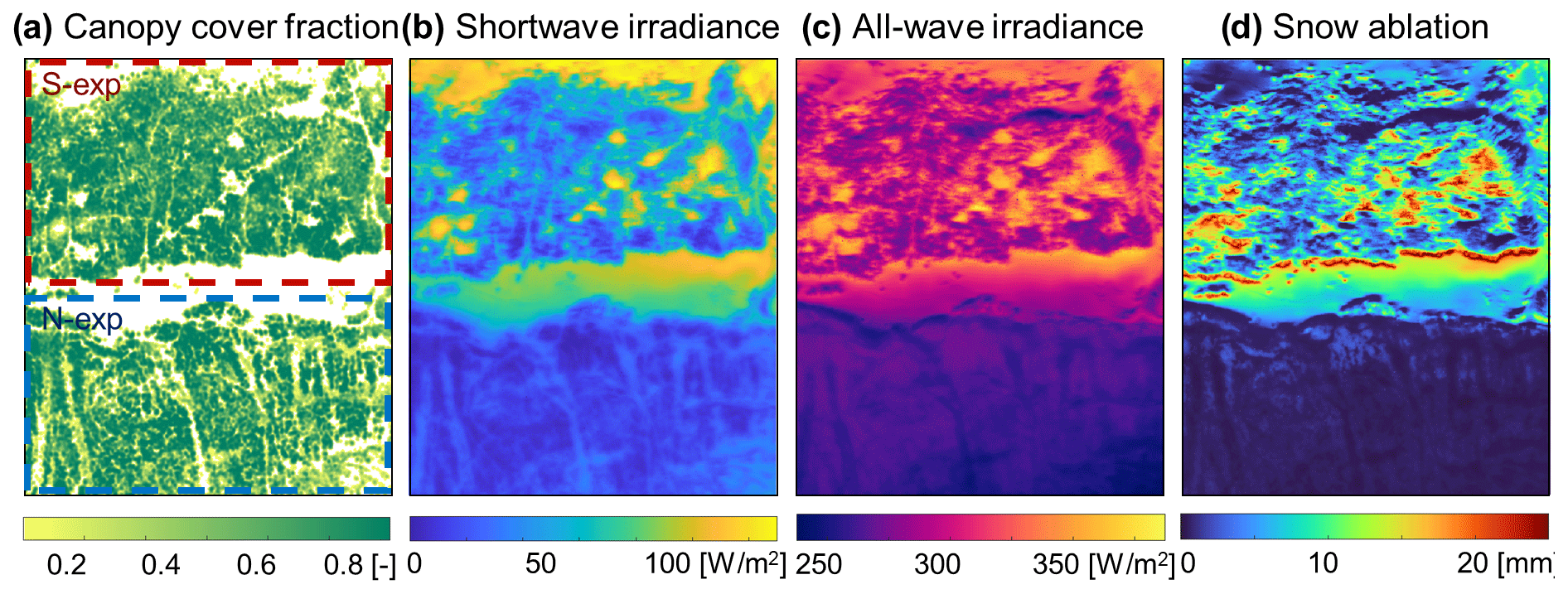
Figure 7 Canopy cover fraction and aspect in the sub-domain (a), average incoming shortwave (b), average all-wave irradiance (c), and cumulative SWE ablation (d) between mid-January and end of February for WY 2019.

In early winter, shortwave irradiance controls all-wave irradiance patterns (Fig. 7b vs. c; see also Fig. S5.2 in the Supplement), and ablation largely matches these patterns (Fig. 7d), confirming that early-season shortwave irradiance is a prerequisite for early-season ablation. Due to topographic shading, only the south-exposed slope receives direct shortwave irradiance at this time of the year. Consequently, topography exerts a primary control on early-season ablation. On top of that, canopy shading affects the distribution of shortwave irradiance, but during times with low solar elevation angles the dependency between canopy structure and direct shortwave radiation is complex. In fact, early in the season the correlation between shortwave irradiance and local canopy cover is rather low (R = −0.52). This, in turn, entails local canopy cover and snow ablation to be uncorrelated as well (R = 0.05). These low correlations imply that early-season ablation may potentially counteract and even disrupt the association of peak SWE patterns and local canopy cover identified in Sect. 3.2 (see Fig. 5).

Shortwave irradiance is, however, not the only flux determining ablation patterns. Figure 7 reveals that some areas above the treeline on the south-exposed slope do not experience early-season ablation, despite the high shortwave radiation input. This indicates that net energy input must be reduced by other negative fluxes. Additionally, the energy balance partitioning plots in Fig. 6 evidence other positive contributions to net energy input to the snowpack. To visualize the spatial structure of these contributions, Fig. 8 shows each individual surface energy balance component (net short- and longwave radiation and sensible and latent heat fluxes) for periods early (Fig. 8a) and late (Fig. 8b) in the season (WY 2019), as well as the corresponding net surface energy flux (Fig. 8c). The spatial distribution of individual energy fluxes and their evolution in time generally conform with findings from Fig. 6, with sensible heat as the only other positive contribution early in the season and longwave transitioning into a positive flux especially at under-canopy locations and later in the season. Overall, Fig. 8 demonstrates how spatial patterns of individual fluxes translate to patterns of net surface energy, which largely match shortwave radiation patterns in both periods. Figure 8d displays correlation coefficients between net surface energy and individual energy balance components as they evolve over the season. The strongest positive correlations to shortwave radiation are confirmed, while correlations to longwave radiation are consistently and increasingly negative. No systematic link between net energy and turbulent fluxes is evident.

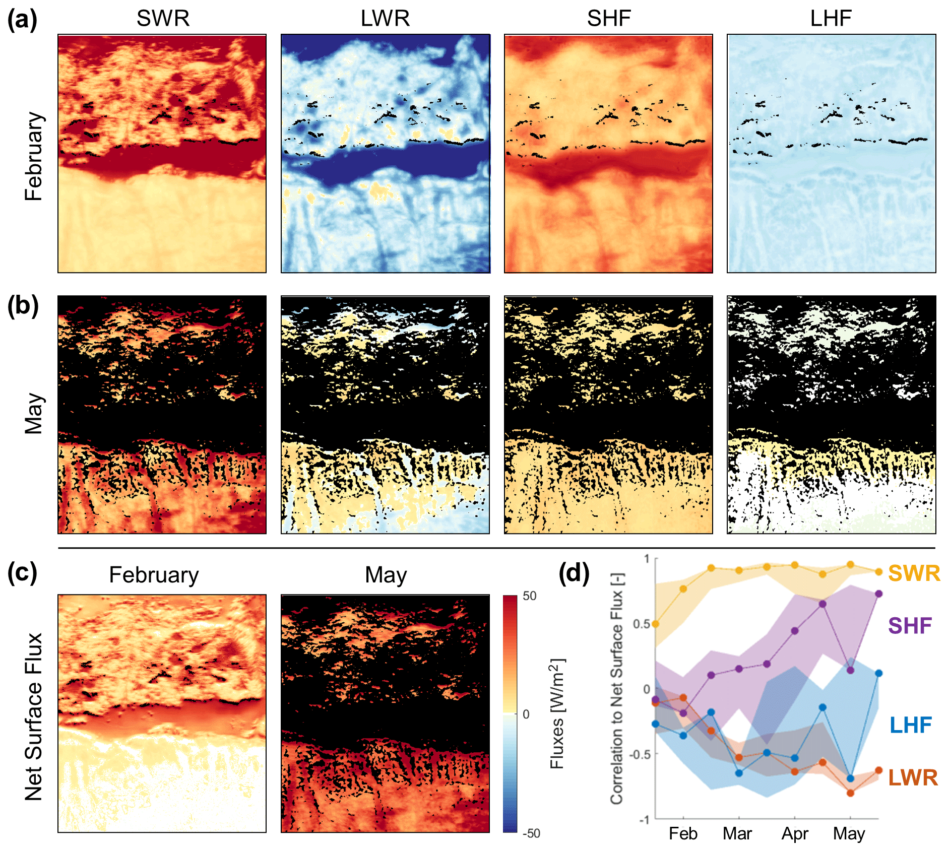
Figure 8 Energy flux partitioning into the four surface energy balance components (net shortwave and longwave radiation, SWR and LWR; sensible and latent heat fluxes, SHF and LHF) for 2 weeks in February (a) and May (b) 2019, respectively, as well as net energy flux at the snow surface (c), areas that have melted out by the time shown are marked black; Correlations (Pearson's R) between individual energy fluxes and net surface energy over the season (d), with lines showing WY 2019 and shaded areas the range of all modelled WYs.

3.5 Impact of meteorological conditions on the temporal consistency of spatial patterns

Meteorological conditions and their variability between years alter the relative magnitude and timing of different processes. By doing so, they can potentially impact the consistency of snow cover dynamics and resulting spatial patterns. Figure 9 shows the spatial distribution of the same snow cover descriptors shown in Fig. 5 but now including three different WYs. Full domain maps of all WYs are available in the Supplement (Figs. S7.1–S7.5). For all snow season descriptors, we find both temporally consistent and inconsistent features. The link between canopy structure and peak SWE is evident in all years, despite stronger imprints of early-season ablation patterns in some years (e.g. 2018 vs. 2019). In fact, the autocorrelation between peak SWE patterns of different years is high (R: 0.94–0.98). In contrast, ablation rate patterns are generally uncorrelated (R: 0.07–0.79). Ablation rate maxima are found at different locations of the domain in different years. For example, maximum ablation rates in WY 2018 were above the treeline on the south-exposed slopes but were in canopy gaps on the north-exposed slope in both WYs 2017 and 2019. Below-canopy areas have comparatively low ablation rates in all years, but differences between slopes are more pronounced in WY 2018 than in 2017 and 2019. These consistencies and inconsistencies are likely affected by differences in the timing of the ablation period.

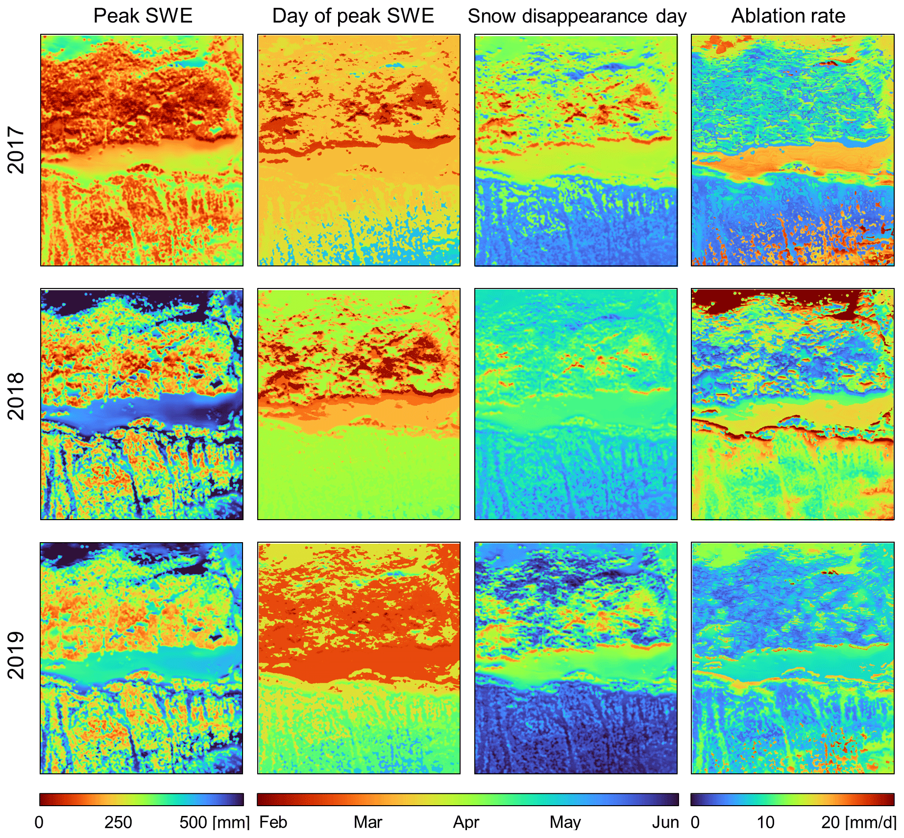
Figure 9 Spatial patterns of snow season descriptors for the sub-domain, including peak SWE (1st column), day of peak SWE (2nd col.), snow disappearance day (3rd col.), and ablation rate (4th col.) during three different WYs, namely 2017 (1st row), 2018 (2nd row), and 2019 (3rd row).

In terms of the timing of peak SWE and snow disappearance, the temporal sequence in which different locations melt out is mostly consistent between years: south-exposed canopy edges and under-canopy locations generally become snow-free first, and snow lasts longest in shaded canopy gaps (i.e. those on north-exposed slopes). However, the timing of and days between both peak SWE and snow disappearance across the domain vary. For example, distribution of peak SWE day in 2019 is, in the first order, bimodal, with a clear separation between the south- and north-exposed slopes; also in 2017, the distribution of peak SWE day is approximately bimodal but in this case with a separation of only the sunny forest edges on the south facing slope, reflecting a considerably smaller number of pixels that exhibit sufficient early-season ablation to prepone peak SWE day relative to all other pixels.

Analogous to our approach in Sect. 3.3, we consider time series at point locations to unravel the process-level mechanisms that cause potential inconsistencies in snow cover descriptor patterns between years (Fig. 10). To better highlight these inter-annual variations, we focus on a set of points located in semi-open conditions on the south-exposed slope, i.e. where they can potentially receive early-season direct shortwave radiation (for locations, see the Supplement Fig. S6.1). These include a point in a large gap, close to the south-facing canopy edge (yellow); a point in a smaller gap (dark red); and two points under relatively sparse canopy in a rather sunny (dark blue) and a shady (cyan) location, respectively. Due to the limited range in local canopy cover at these points, the differences in accumulation caused by interception are less pronounced than for the examples shown in Sect. 3.3 (cf. Fig. 10 vs. Fig. 6). Yet, these points experience different drivers of ablation and therefore react differently to variations in meteorological conditions between the years.

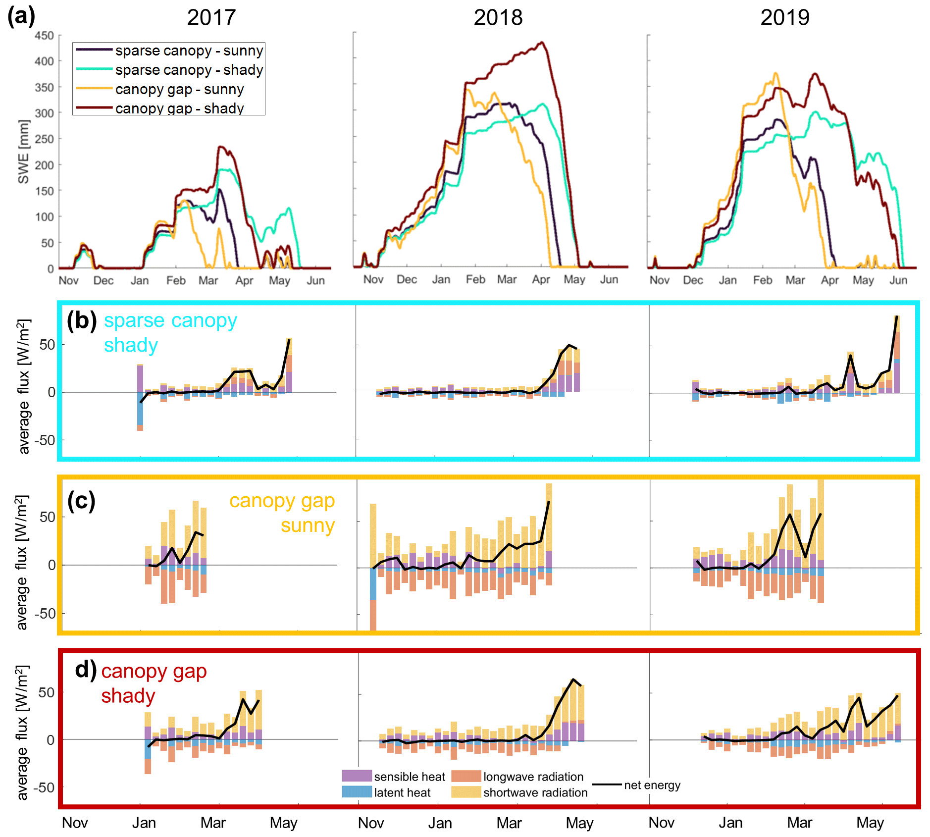
Figure 10 Impact of meteorological conditions illustrated by comparing three different WYs (columns), including (a) SWE evolution at four example points (locations see S3) and surface energy partitioning pathways at three of these, i.e. (b) a shady sparse canopy location, (c) a sunny canopy gap location, and (d) a shady canopy gap location.

Firstly, we note that accumulation patterns (i.e. peak SWE) vary between years based on the timing of the first ablation events relative to the timing of peak SWE, particularly whether or not considerable ablation events occur during the accumulation period (Fig. 10a). In 2019, when all major snowfall events occur prior to the first melt episode, gaps feature the highest peak SWE, corresponding to low interception losses (yellow and red). In 2017 in contrast, overall accumulation is low, and substantial melt precedes the last major accumulation event, which is sufficient to cause melt-out at some of the most sun-exposed locations; peak SWE at the sunny canopy gap point (yellow) is now thus the lowest of the four points considered. It should be noted that, for all WY's considered here, onset of full snow cover happened roughly simultaneously across the entire model domain; early ablation events leading to partial melt-out prior of the onset of full snow cover (not shown but observed, for example, in WY 2016) would obviously further complicate peak SWE patterns.

Second, we note that the relative timing of snow disappearance between years can vary across the domain, based on the availability of melt energy over the course of the season (Fig. 10a). Points that normally receive early-season shortwave irradiance (i.e. the dark blue and the yellow point) melt out later in WY 2018 compared to 2019, because less shortwave irradiance is available in February (see strong positive shortwave contributions in Fig. 10c). In contrast, points in shadier locations (cyan and red) melt earlier in WY 2018 because of the consistently warmer and sunnier weather in spring compared to 2019 (see earlier switch to both positive shortwave and longwave contributions in Fig. 10b and d). The opposed effect of these differences in meteorological conditions causes snow disappearance day of the four points to be much closer in WY 2018 than in 2019. The overall melt-out patterns will thus vary between WYs, even if the dominating fluxes at each specific location remain approximately consistent (Fig. 10b–d).

4 Discussion

4.1 Process-level insights

Spatio-temporal snow cover dynamics and associated snow accumulation and ablation patterns are a result of superimposed processes that themselves vary as a function of both time-invariant physiographic features (vegetation, topography) and time-varying meteorological conditions. While the phenological analysis of snow season descriptors presented in Sect. 3.1–3.2 paints a complex picture of snow distribution patterns, the process-level analysis in Sect. 3.3–3.5 allowed us to attribute the processes that underlie these patterns. The main takeaway from this work is that patterns of snow season descriptors and their inter-seasonal consistency can only be explained by considering all three factors, canopy structure, topography, and meteorology, as well as their interaction throughout the snow season.

Snow distribution patterns at any point in time arise from an interplay between accumulation and ablation patterns. For the study site considered here, our analysis showed that snow cover dynamics result from the superposition of (1) a pattern that is temporally static and dependent on canopy structure alone, with more snow where there is less canopy (i.e. accumulation mostly controlled by interception) and (2) a time-varying pattern with complex dependencies on canopy structure, solar position, weather, and topography, with an overall tendency for faster ablation where there is less canopy (i.e. melt mostly controlled by shortwave radiation). Depending on the relative strength of each of both signals, three regimes of snow cover dynamics are principally possible:

• R1.

  Snow distribution can be described as a function of canopy structure alone throughout the whole season. This is the case when accumulation creates a strong signal, and ablation patterns are too homogeneous or too weak to override this signal, so areas that accumulate less snow also melt out first.

• R2.

  Snow accumulation patterns can be described as a function of canopy structure during the accumulation period, but those patterns will be overridden by ablation patterns during the ablation period. Consequently, snow disappearance date exhibits no simple relationship with canopy structure.

• R3.

  Early-season ablation inhibits formation of simple snow accumulation patterns, and snow distribution patterns remain weakly correlated with canopy structure throughout the entire season.

Based on these regimes and using WY 2018 as an example, Fig. 11c shows a conceptual subdivision of our model domain into four zones. Zone A does not feature early-season ablation and exhibits snow disappearance patterns that carry the imprint of local canopy cover; Zone B is characterized by substantial cumulative early-season ablation amounts (Fig. 11a); Zones C and D largely lack early ablation but exhibit fewer clear linkages between canopy cover and snow disappearance day (Fig. 11b). Note that Zones C and D are treated separately due to elevational differences. As a crosscheck, we computed the temporal evolution of the correlation coefficient between SWE and local canopy cover for each of the four zones separately (Fig. 11d). As expected, Zone A (R1) features a strong negative correlation between SWE and local canopy cover throughout the entire season; Zone D (R2) exhibits a similarly strong correlation at the beginning of the season which then degrades during ablation season; and Zone B (R3) exhibits a weaker correlation even early in the season, where each ablation episode degrades and where each interception event improves the correlation, until the ablation season causes the correlation to collapse more permanently. Zone C seems to show characteristics of R2 in 2018 but of R3 in 2016, which implies that the regime found at a specific location may not be consistent from year to year.

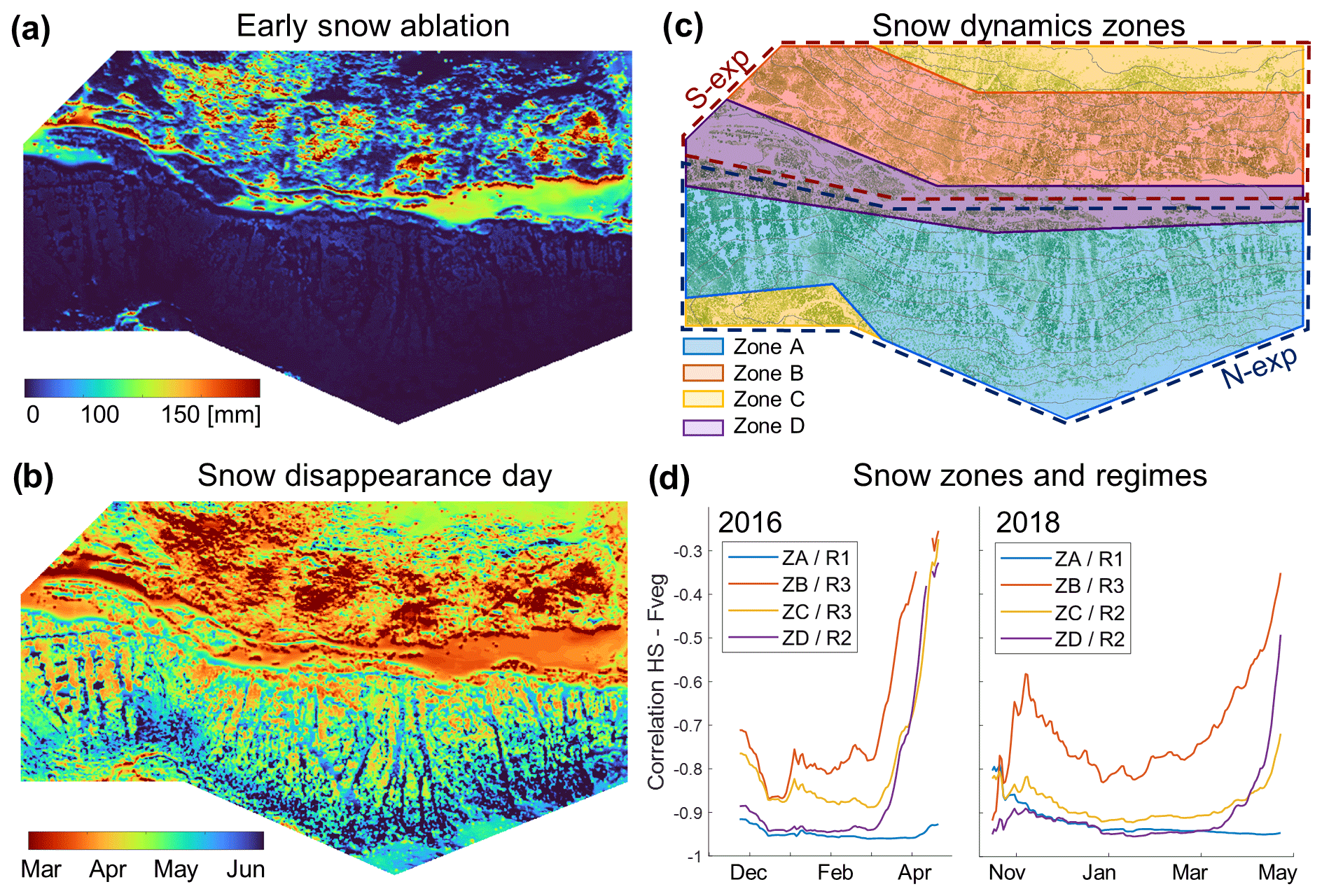
Figure 11 Conceptual subdivision of study domain into snow cover evolution regimes, the identification of which is based on maps of cumulative SWE ablation between mid-January and mid-March (a) and snow disappearance day (b) in WY 2018. Resulting zones (c) and evolution of the correlation coefficients between snow depth and vegetation cover fraction in these for WYs 2016 and 2018, resulting in the attribution to a specific regime (d).

The co-occurrence of different regimes across our study domain is a consequence of topography, because early-season shortwave irradiance is a prerequisite for regime 3, while its absence is a prerequisite for regime 1. North-exposed slopes are prone to falling into regime 1, while south-exposed slopes tend to conform with regime 3. Regime 2 is less evident in our example but most likely to be found in flat areas with large canopy gaps, where early-season ablation is not expected, but substantial melt energy gradients can evolve during ablation. The impact of inter-annual variability in meteorological conditions can lead to the same locations hosting different regimes in different WYs: differences result from either weaker accumulation patterns or variations in magnitude and timing of shortwave irradiance. This finding is in line with Lundquist and Flint (2006), who attributed variability in snowmelt patterns between years with early and late snowmelt onset to differences in topographic shading. Our analysis also furthers the conceptual framework presented by Lundquist et al. (2013). Based on site-scale simulations of the net radiative balance, they established timing of early melt, determined by the climatological temperature at a site, as the primary control of whether denser forest would generally accelerate or delay snowmelt through the prevalence of longwave radiation enhancement or shading, respectively. Our approach, involving more processes and detailed canopy structure information, confirms the importance of early-season ablation but demonstrates the additional key role of shortwave radiation patterns in determining snow dynamics regimes at smaller spatial scales.

The categorization of snow cover dynamics into regimes provides a context to temporal snapshots of snow distribution patterns, such as those derived from singular lidar datasets. The temporal evolution of correlation coefficients (Fig. 11d) corroborates findings from Koutantou et al. (2022), who used maps of modelled sub-canopy irradiance to explain why snow distribution patterns exhibited different dependencies on canopy structure at their north- and south-exposed survey sites. A decay of the correlation between snow distribution and canopy structure between two lidar acquisitions in spring was also observed by Mazzotti et al. (2019a) for sites with less topographic variability. In general, our process-level insights explain why these correlations can vary between years and regimes, as shown in this study, and hence why different studies may have observed different and sometimes inconsistent dependencies between snow and canopy variables, depending on when and where data were acquired (e.g. Safa et al., 2021; Currier and Lundquist, 2018).

4.2 Implications and applications

The process-level insights discussed in the previous section have important implications for a variety of contexts in which small-scale variability of forest snow cover dynamics is relevant. We elaborate on three such examples in the following.

Firstly, our findings indicate that strategies to account for sub-grid variability in coarser-resolution models that are intended for application to sub-alpine environments need to account for variations in canopy structure, topography, and meteorology. This is particularly the case at sub-kilometre model resolutions, where variability in driving meteorological conditions induced by topography is at least partially resolved (e.g. through temperature lapse rates and orographic precipitation gradients), while variability in snow cover dynamics caused by canopy structure occurs at much smaller spatial scales and needs to be parameterized (Clark et al., 2011). The south-exposed slope in our model domain featured stronger variability and more complex patterns of snow cover descriptors than the north-exposed slope, with impacts on the evolution of fractional snow-covered area in grid cells that include such terrain. To our knowledge, sub-grid variability parameterizations that incorporate these effects are inexistent to date (Dickerson-Lange et al., 2015; Mazzotti et al., 2021; Schneider et al., 2020), but their development is a promising avenue for further model improvement. However, recent studies have suggested tiling schemes based on fine-scale canopy structure as an alternative approach to representing sub-grid variability (Broxton et al., 2021; Currier et al., 2022), in line with our findings.

Secondly, our simulations evidence a strong complexity in ecohydrologically relevant processes across a still relatively limited study domain. The large range of snow cover durations observed creates spatial variability in ground insulating properties and soil temperatures. Snow water input to the ground also exhibits strong spatial heterogeneity due to variability in snow melt magnitudes and rates, with further influences on soil moisture evolution. As soil conditions control a wide range of biophysical processes (Neumann et al., 2019; Stark et al., 2020; Harpold, 2016), their spatial heterogeneity potentially implies strong variability of habitat characteristics across relatively small spatial scales (Niittynen et al., 2018). It is also possible that the observed process variability affects ecologically relevant snow properties such as surface layer density (Boelman et al., 2019; Gilbert et al., 2017) or the formation of ice layers in the snowpack (Rasmus et al., 2018). This is an unexplored research topic to date, as resolving these internal snowpack processes would require a more sophisticated snow scheme than available in FSM2. Coupling of detailed canopy representation to snow physics models such as Crocus (Vionnet et al., 2012; Lafaysse et al., 2017) and SNOWPACK (Bartelt and Lehning, 2002; Lehning et al., 2002; Gouttevin et al., 2015) would hence be a prerequisite. Overall, our results advocate that small-scale landscape heterogeneity needs to be considered when addressing snow-related ecohydrological questions in sub-alpine forested environments.

Lastly, process-level insights allow us to extrapolate our findings spatially and temporally. While it is known that forest snow cover dynamics differ across climates (Lundquist et al., 2013; Dickerson-Lange et al., 2021; Safa et al., 2021), the same underlying processes are active everywhere. The snow distribution patterns found in this study may thus not be directly transferrable to other regions, but improved understanding of how physiographic and meteorological factors interact with one another allows us to better predict where and when certain processes will prevail. Consequently, we expect the prevalence of specific snow dynamics regimes to vary with latitude, regional temperature, and snowfall characteristics. Likewise, these insights enable improved prediction of how patterns may shift following environmental change. Our findings suggest, for instance, that canopy removal may have the opposite effect in different topographic locations, i.e. earlier and faster ablation on south-exposed slopes but longer snow retention in north-exposed ones. Warmer temperatures earlier in the season favour longwave-radiation driven ablation (Lundquist et al., 2013), shifting the relative timing of shortwave vs. longwave-radiation driven ablation. Such a shift which would likely accentuate accumulation patterns and thus alter melt-out patterns on south-exposed slopes but only show minor impacts on north-exposed slopes.

The use of hyper-resolution models in the context of forest management and climate change impact studies is still underexploited but should be encouraged in the future as only process-based models allow predictions that extrapolate from currently known conditions. Indeed, forest snowpacks in sub-alpine regions reside at climate-sensitive elevations (Schöner et al., 2019; Pepin et al., 2015), and forest structural change is widely and rapidly happening (Albrich et al., 2020; Goeking and Tarboton, 2020).

4.3 Assets, limitations, and outlook

Considerations in Sect. 4.1 and 4.2 underline the assets of a process-based modelling approach in terms of its capabilities to resolve individual process dynamics. Additionally, modelling allowed us to obtain spatially and temporally continuous information, which is not feasible with today's observation technology. Most ALS-based snow datasets that cover large areas are available for only a few temporal snapshots (Safa et al., 2021; Currier and Lundquist, 2018; Harpold et al., 2014; Broxton et al., 2019), while existing attempts to acquire snow distribution time series are very limited in spatial extent and mostly cover one winter season only (Koutantou et al., 2022; Broxton et al., 2020). Process-level data that are both spatially and temporally explicit are even more scarce and extremely challenging to obtain (Moeser et al., 2015; Malle et al., 2019, 2021; Mazzotti et al., 2019b). Model application, in contrast, is only limited by the availability of driving meteorological data and surface datasets and is thus potentially applicable to extensive spatial and temporal domains.

Modelled process dynamics, however, can only yield satisfactory estimates of reality if the model representations of the processes involved are sufficiently accurate. For this study, we used FSM2, which we believe to be particularly suited given previous validation efforts demonstrating the model's capability to accurately represent individual processes related to the snowpack surface energy balance (Mazzotti et al., 2020a). Yet, we acknowledge that our findings depend on modelling choices, and results might vary when using alternative models or process parameterizations. Therefore, the modelling community should strive for continued improvement. On the one hand, the representation of some processes could still be improved, and associated uncertainties should be evaluated systematically across the full range of canopy structure and topographic diversity of the application domains of interest. This is especially the case for processes involving snow in the canopy (Lundquist et al., 2021; Lumbrazo et al., 2022). Moreover, while Mazzotti et al. (2020a) could infer spatial patterns of snow surface fluxes from their data, direct validation of turbulent fluxes is challenging even with recent measurement techniques (see, for example, Conway et al., 2018; Peltola et al., 2021; Haugeneder et al., 2022).

Some processes, such as snow transport by wind and gravitational redistribution by avalanches in steep slopes, are not represented in the model framework used here. These processes significantly drive snow distribution patterns in open alpine terrain but are assumed to have a smaller impact on fine-scale patterns in forests. Efforts to couple FSM2 to snow redistribution models (e.g. Liston and Sturm, 1999; Bernhardt and Schultz, 2010) are ongoing. Additionally, mass and energy exchange between neighbouring locations may become relevant at hyper-resolutions (Schlögl et al., 2018), and lateral coupling would likely improve the representation of expanding snow-free areas in spring. Coupling to a soil or ecohydrological model (Fatichi et al., 2012; Tague and Band, 2004) would further extend the potential applications of hyper-resolution forest snow schemes beyond just snow cover dynamics. Finally, a major challenge concerns the estimation of model parameters that are potentially variable in space. This approach was not pursued in this study but has been shown to considerably increase the benefits of calibration efforts (Wrzesien et al., 2022). Approaches to automate model calibration across the full range of canopy structures and topographic settings may thus further improve the skill of models like FSM2.

In the longer term, combining hyper-resolution models and observations to leverage their complementary assets is likely the most promising avenue to advance our understanding of forest snow cover dynamics in complex terrain. Plausibility checks as presented in Sect. 2.3 are indispensable for the verification of model use cases, as well as for continued model enhancement and refinement, and there is potential for improvement here as well. For instance, the use of RGB satellite data to validate melt-out patterns (Sect. 2.3) is promising despite limited visibility of snow under the canopy. Automated algorithms to extract snow cover information from RGB imagery are not currently applicable to forested complex terrain (Deschamps-Berger et al., 2020; Gascoin et al., 2019) but would encourage the use of such datasets for this purpose. If respective workflows are continuously improved, enabling simulations and observations to be used in tandem and to benefit from each other (e.g. through data assimilation approaches), hyper-resolution model applications at large temporal and spatial scales in the contexts discussed in Sect. 4.2 promise advances in ecohydrological and land surface modelling research.

5 Conclusions

This study represents the first multi-year application of a hyper-resolution forest snow model capable of resolving tree-scale processes within a sub-alpine valley, aimed at investigating how snow cover dynamics and the underlying processes are shaped by the interplay of (1) canopy structure, (2) terrain, and (3) meteorological conditions. The chosen approach yielded process-level insights that could not be obtained based on snow distribution datasets alone.

Our findings evidenced that these three factors must be considered when attempting to explain spatio-temporal snow cover dynamics. Canopy structure exerts the primary control on accumulation patterns, yet the resulting snow distribution can be disrupted by ablation patterns, which are primarily driven by the distribution of shortwave radiation. Because shortwave radiation exhibits complex canopy dependencies and tends to counteract accumulation patterns, it is the timing of radiation relative to the strength of the accumulation patterns that determines whether accumulation patterns persist until melt-out or whether they are overridden by more complex ablation patterns. Since amount and timing of shortwave irradiance are largely controlled by topography, south-exposed slopes are more prone to accumulation patterns being superseded by ablation patterns even early in the season compared to north-exposed slopes, where accumulation patterns likely persist throughout melt-out. Finally, variability in meteorological conditions alters the relative strength of processes (accumulation, direct insolation, longwave-driven ablation) and can thus cause snow accumulation and ablation pattern inconsistencies between years. This framework explains why snow distribution patterns in some areas exhibit a strong relationship with canopy structure, while they do not in other areas, and why this can change between years.

Process understanding gained from this work provides context to existing snow distribution datasets and a proof of concept for the continued development and application of hyper-resolution modelling approaches to forest-snow-related research in complex terrain. Potential usages include questions that revolve around developing sub-grid variability parametrization in coarse-resolution models, exploring the ecohydrological effects of the observed small-scale snow dynamics, and the application of hyper-resolution models in environmental change impact studies.