Uncertainty estimation of regionalised depth–duration–frequency curves in Germany

The estimation of rainfall depth–duration–frequency (DDF) curves is necessary for the design of several water systems and protection works. These curves are typically estimated from observed locations, but due to different sources of uncertainties, the risk may be underestimated. Therefore, it becomes crucial to quantify the uncertainty ranges of such curves. For this purpose, the propagation of different uncertainty sources in the regionalisation of the DDF curves for Germany is investigated. Annual extremes are extracted at each location for different durations (from 5 min up to 7 d), and local extreme value analysis is performed according to Koutsoyiannis et al. (1998). Following this analysis, five parameters are obtained for each station, from which four are interpolated using external drift kriging, while one is kept constant over the whole region. Finally, quantiles are derived for each location, duration and given return period. Through a non-parametric bootstrap and geostatistical spatial simulations, the uncertainty is estimated in terms of precision (width of 95 % confidence interval) and accuracy (expected error) for three different components of the regionalisation: (i) local estimation of parameters, (ii) variogram estimation and (iii) spatial estimation of parameters. First, two methods were tested for their suitability in generating multiple equiprobable spatial simulations: sequential Gaussian simulations (SGSs) and simulated annealing (SA) simulations. Between the two, SGS proved to be more accurate and was chosen for the uncertainty estimation from spatial simulations. Next, 100 realisations were run at each component of the regionalisation procedure to investigate their impact on the final regionalisation of parameters and DDF curves, and later combined simulations were performed to propagate the uncertainty from the main components to the final DDF curves. It was found that spatial estimation is the major uncertainty component in the chosen regionalisation procedure, followed by the local estimation of rainfall extremes. In particular, the variogram uncertainty had very little effect on the overall estimation of DDF curves. We conclude that the best way to estimate the total uncertainty consisted of a combination between local resampling and spatial simulations, which resulted in more precise estimation at long observation locations and a decline in precision at unobserved locations according to the distance and density of the observations in the vicinity. Through this combination, the total uncertainty was simulated by 10 000 runs in Germany, and it indicated that, depending on the location and duration level, tolerance ranges from ± 10 %–30 % for low-return periods (lower than 10 years) and from ± 15 %–60 % for high-return periods (higher than 10 years) should be expected, with the very short durations (5 min) being more uncertain than long durations.

1 Introduction

Design precipitation volumes at different duration and frequencies, also known as depth–duration–frequency (DDF) curves, are necessary for the design of many water-related systems and facilities. These curves are typically generated by fitting a theoretical distribution to the rainfall extremes (either annual extremes (AMS) or extremes above a threshold (POT)) derived for specific duration intervals at observed locations. Mostly, a generalised extreme value distribution with three parameters (location, scale and shape) is preferred for such applications (Koutsoyiannis, 2004a, b). An adjustment of the rainfall extremes over different duration intervals is also considered either before fitting the theoretical distribution (as in Koutsoyiannis et al., 1998) or after (as in Fischer and Schumann, 2018). As the fitted theoretical distribution can be used to describe the DDF values only at observed locations, regionalisation techniques are applied to estimate these distributions at unobserved locations. The estimation of a regional distribution based on the index method as proposed by Hosking and Wallis (1997) is one of the most used methods in the literature (Burn, 2014; Forestieri et al., 2018; Perica et al., 2019), followed by the kriging interpolation of the parameters describing these theoretical distributions (Ceresetti et al., 2012; Shehu et al., 2023; Uboldi et al., 2014).

Nevertheless, the procedure for the derivation of DDF curves is subjected to different sources of uncertainty which can affect the confidence level of the estimated design values. Such sources of uncertainties include measurement errors, choice of distribution, short observation length, non-representativeness of point measurements for the spatial dependency of extremes and instationarity due to the climate change (Marra et al., 2019a). So far, for DDF curves in Germany there has been no objective quantification of the uncertainty but only approximative guessed tolerance ranges between 10 %–20 % (depending on the return period) that should account for the measurement errors, uncertainties in the extreme value estimation and regionalisation, and for the climate variability (Junghänel et al., 2022). The tolerance ranges are kept constant throughout duration levels and locations; nevertheless, such tolerance ranges are expected to be higher for very short observations and high-return periods (Poschlod, 2021) especially for short durations and drier climate (Marra et al., 2017). Therefore, there is a need to perform different simulations in order to quantify the tolerance ranges (uncertainty) dependent on duration, location and return period. In this paper, the focus is on developing a framework that accounts for uncertainties due to short observation lengths and non-representativeness of point measurements for spatial dependencies of extremes. Once a framework is developed, it can be used to investigate the role of distribution choice as in Miniussi and Marra (2021) or the role of future climate as in Poschlod (2021).

In the literature, parametric or non-parametric bootstrapping resampling techniques are used to quantify tolerance ranges of DDF curves. Overeem et al. (2008) were one of the first to include the uncertainty of such curves by including only the uncertainty of generalised extreme value (GEV) parameters estimated by a regional bootstrap procedure (sample variability). In their study, extremes from a homogeneous region were pooled together to estimate regional probability distribution, which resulted in a narrower uncertainty range at observed locations. Overeem et al. (2009) proposed a bootstrapping technique where the same years for all the observed points were resampled together in order to maintain the spatial dependency of the extremes. Uboldi et al. (2014) went a step further and accounted spatial dependency when performing the bootstrapping for each location: extremes from near observations have a higher probability to be resampled at a specific location than the ones from far away. Typically, the bootstrapping procedures are implemented together with the index-based regionalisation as proposed by Hosking and Wallis (1997). Examples in the literature of such applications are for instance in Burn (2014) and Requena et al. (2019) in Canada where the uncertainty is computed from the confidence intervals of a parametric bootstrap procedure or in Chaudhuri and Sharma (2020), Notaro et al. (2015), Tfwala et al. (2017) and Van de Vyver (2015) where a Bayesian framework is employed to estimate the uncertainty of DDF curves at different duration levels. Mostly, the uncertainty is derived from bootstrap procedure where the 95 % or 90 % confidence interval width is used as a measure of precision: the lower the confidence interval width, the more precise the estimates are. However, the spatial structure of uncertainties is not well considered in the index-based regionalisation: first, no uncertainty of the index itself is considered and propagated, and second, there is no measure of how uncertain the locations further away from observations are. Therefore, local resampling of extreme values (to account for sample variability) is not enough to describe the spatial structure of uncertainty; instead, spatial simulations are needed. Alternatively, remote sensing data, i.e. satellites or weather radar data, provide spatially continuous indirect measurements of rainfall intensities or volumes (Marra et al., 2019a). However, their shortcomings are related to the short available dataset, the inability of the remote sensing dataset to capture accurately intensities, and the lack of a true observed dataset to validate the methods applied. While remote sensing provides a valuable tool and more research is performed in tackling better the uncertainties, at the moment, DDF curves from station observations still represent the standard procedure, and hence, a method to estimate the spatial structure of uncertainties based on these observations is required.

In kriging, when regionalising from point values, the variance of the estimations can be used as a measure of the uncertainty for unobserved locations. This estimation can either be parametric (multi-Gaussian process) or non-parametric (indicator kriging). It is widely accepted that the kriging system can capture only the local uncertainty (providing information at one location at a time conditioned to other observations in the vicinity) and not the spatial one (providing a measure of uncertainty about the unsampled values taken altogether in space rather than one by one), the estimated uncertainty is dependable on the data configuration rather than on the value itself, and lastly it fails to preserve the high spatial variability of the target variable (Cinnirella et al., 2005; Deutsch and Journel, 1998; Goovaerts, 1999a, 2001; Lin and Chang, 2000). As stated in Liao et al. (2016), the spatial uncertainty is more important (bigger) than the local uncertainty. Therefore, solutions for the estimation of the spatial uncertainties in geostatistics are stochastic simulations with equiprobable realisation of the target variable in space. The main assumption of the stochastic simulations is the generation of equiprobable realisations in space while maintaining certain global statistics of the target variable, for instance, the histogram of the observed values and the semi-variogram (herein referred to as variogram for simplicity), which describes the spatial dependency of the variable variance on the distance between the observations. The stochastic simulations present a trade-off: on the one hand, they provide more spatial variable fields than kriging (which is known for its smoothing properties), and on the other hand, because the goal is to maintain the global statistics, they may suffer from larger errors at the local scale. Another advantage of stochastic simulations is the ability to directly compute the confidence intervals for the target variable, while in kriging interpolation, the confidence intervals are computed from the kriging variance assuming a normal distribution of the errors.

Examples of different stochastic simulations are the sequential Gaussian simulations (SGSs) (Cinnirella et al., 2005; Emery, 2010; Ersoy and Yünsel, 2009; Gyasi-Agyei and Pegram, 2014; Jang, 2015; Jang and Huang, 2017; Liao et al., 2016; Poggio et al., 2010; Ribeiro and Pereira, 2018; Szatmári and Pásztor, 2019; Varouchakis, 2021; Yang et al., 2018), sequential indicator simulations (SISs) (Bastante et al., 2008; Goovaerts, 1999b; Luca et al., 2007), simulated annealing (SA) (Goovaerts, 2000; Hofmann et al., 2010; Lin and Chang, 2000) and turning bands (TBs) (Namysłowska-Wilczyńska, 2015). As seen, the most preferred stochastic simulation in the literature is the SGS, due to its simplicity, followed by the SIS and then by SA. Alternatively a stochastic random mixing (as stated in Bárdossy and Hörning, 2016) with spatial dependency modelled by copulas (Haese et al., 2017) or a collocated co-kriging simulation (Bourennane et al., 2007) can also be applied. However, geostatistical simulations remain the preferred choice in the literature for estimating spatial uncertainty, although the main application is in the geosciences field, with very few applications in rainfall modelling, and to the authors' knowledge, no application in the regionalisation of extreme design rainfall. Therefore, geostatistics becomes a useful tool to estimate and analyse the estimation of DDF uncertainties at observed and unobserved locations. The question of which stochastic simulation is more appropriate for extreme design rainfall is naturally raised.

As stated, because of its simplicity, the SGS is a very popular method in estimating spatial uncertainty in geostatistics. In the SGS approach, each simulation is considered a realisation of the multivariate Gaussian process; hence, it is strictly required for the target variable to be multivariate normal. As discussed in Deutsch and Journel (1998), the testing of the multivariate normality is a difficult task, which, depending on the case at hand, can be very time and computationally expensive and hence is not usually tested. Typically, studies in literature include a transformation to normal distribution in order to ensure that the target variable is at least univariate normal. Another disadvantage of the normalisation needed for the SGS application is that the upper and lower tail of the transformed variable will cause an under/overestimation of these values, and hence, an extrapolation to lower and upper bounds is required. Contrary to the SGS, the sequential indicator simulations (SISs) do not need a prior assumption on the multivariate normality of the target variable, and it is more suitable for observed values that do not exhibit bivariate normal properties. The SIS is a conditional simulation based on the indicator kriging theory, which provides the probability that a location has to exceed a certain threshold. The number of thresholds considered should be more than 5 but lower than 15 as suggested by Luca et al. (2007). For each of the selected thresholds, a variogram is fitted to the portion of the data following under this threshold, and it is used for the sequential simulation. A disadvantage of the SIS is that, if many threshold classes are presented, order relationship problems will arise on the obtained realisations (Deutsch and Journel, 1998; Journel and Posa, 1990), which are more emphasised if empty thresholds are included (Luca et al., 2007). Another disadvantage of the SIS is that mainly it has been used together with simple and ordinary kriging theory (Deutsch and Journel, 1998; Journel and Posa, 1990), and no application of the SIS in an external drift or universal kriging has been reported (to authors knowledge) in the literature. Alternative to the SGS and SIS stochastic simulations, the simulated annealing (SA) can be also implemented to alternate and generate conditional images of a continuous target variable. The main idea in the implementation of the SA is a numerical algorithm which continuously perturbs an image until an objective criterion is reached. The optimisation function can include only one criterion (typically the global statistics) or multiple criteria depending on the application at hand. For instance, Goovaerts (2000) included three criteria: the local estimation of the variable, the observed histogram and the variogram. The advantage of the SA is that no prior assumption of the normality is required (as the observed histogram is reproduced) and that it allows a degree of flexibility for realisations that does not exactly match the objective criteria. On the other hand, the disadvantages of the SA include the prior selection of the objective criteria carefully and, depending on the application, the high computational time.

In our previous study, Shehu et al. (2023) investigated different methods and datasets in Germany for the local estimation of the DDFs from station data and different regionalisation methods for the estimation of the DDFs at ungauged locations. The study revealed that kriging interpolation of long observation records (more than 40 years) with a denser network of short observations as an external drift delivered the best cross-validation results for return periods higher than 10 years. Therefore, apart from the stochastic simulations that account for the spatial uncertainty, more simulations are needed to tackle other sources of uncertainties for the estimation of DDF curves, such as sample variability, variogram estimation and the combination with an external drift. For this purpose, the SGS and SA will be implemented and investigated for their suitability in generating spatial simulations for DDF curves. Once a best method is chosen for this purpose, different experiments are conducted based on non-parametric bootstrapping techniques to investigate how each of the uncertainty components is propagated into the final DDF curves and if some components are more dominant than others. Lastly, based on the most important components, a framework for estimating the total uncertainty in regionalised DDF curves (both at observed and unobserved locations) is proposed.

The paper is organised as follows: first, in Sect. 2, the data and methods for the estimation and regionalisation of DDF curves are explained (Sect. 2.1 and 2.2), followed by the necessary transformation to normality in Sect. 2.3 and testing the bi-Gaussian conditions in Sect. 2.4. Then, an introduction to the main uncertainty sources considered here is given in Sect. 3, and the main methods to tackle each of the uncertainty sources are given in Sect. 3.1 to 3.3. An overview of the experiments and how the uncertainty is measured in terms of both accuracy and precision is described in Sect. 3.4. The results are summarised in Sect. 4, where first a comparison of the two spatial simulations techniques is investigated (Sect. 4.1) and later uncertainty results of different experiments for unobservation locations and for the whole German region are shown respectively in Sect. 4.2 and 4.3. Lastly, conclusions and the best framework to tackle uncertainties for DDF curves in Germany are discussed in Sect. 5.

2 Study area and data processing

The investigation is carried out for Germany, as shown in Fig. 1, together with the two rainfall measuring networks from the German Weather Service (DWD) used for the uncertainty analysis. They are grouped in LSs (long recording stations) – tipping bucket sensors with 1 min temporal resolution, 0.1 mm accuracy, 2 % uncertainty and observation lengths from 40–80 years, and in SSs (short recording stations) – digital sensors with 1 min temporal resolution, 0.01 accuracy, 0.02–0.04 mm uncertainty and observation length from 10–35 years. An overview of the data from these two networks is given in Shehu et al. (2023). For both networks, the 1 min time steps are aggregated to 5 min, and then the annual maximum series (AMS) is extracted for each station for 12 durations levels from 5 min to 7 d. To avoid the underestimation of the rainfall depth due to fixed accumulation periods of 5, 10 and 15 min, correction factors of 1.14, 1.07 and 1.04 were used for the AMS of these durations according to the regulations in DWA-531 (DWA, 2012). Next, as described in Shehu et al. (2023), a jump elimination according to sensor changes is performed as by DVWK (1999), in order to ensure the stationarity of AMS at most stations for different duration levels.

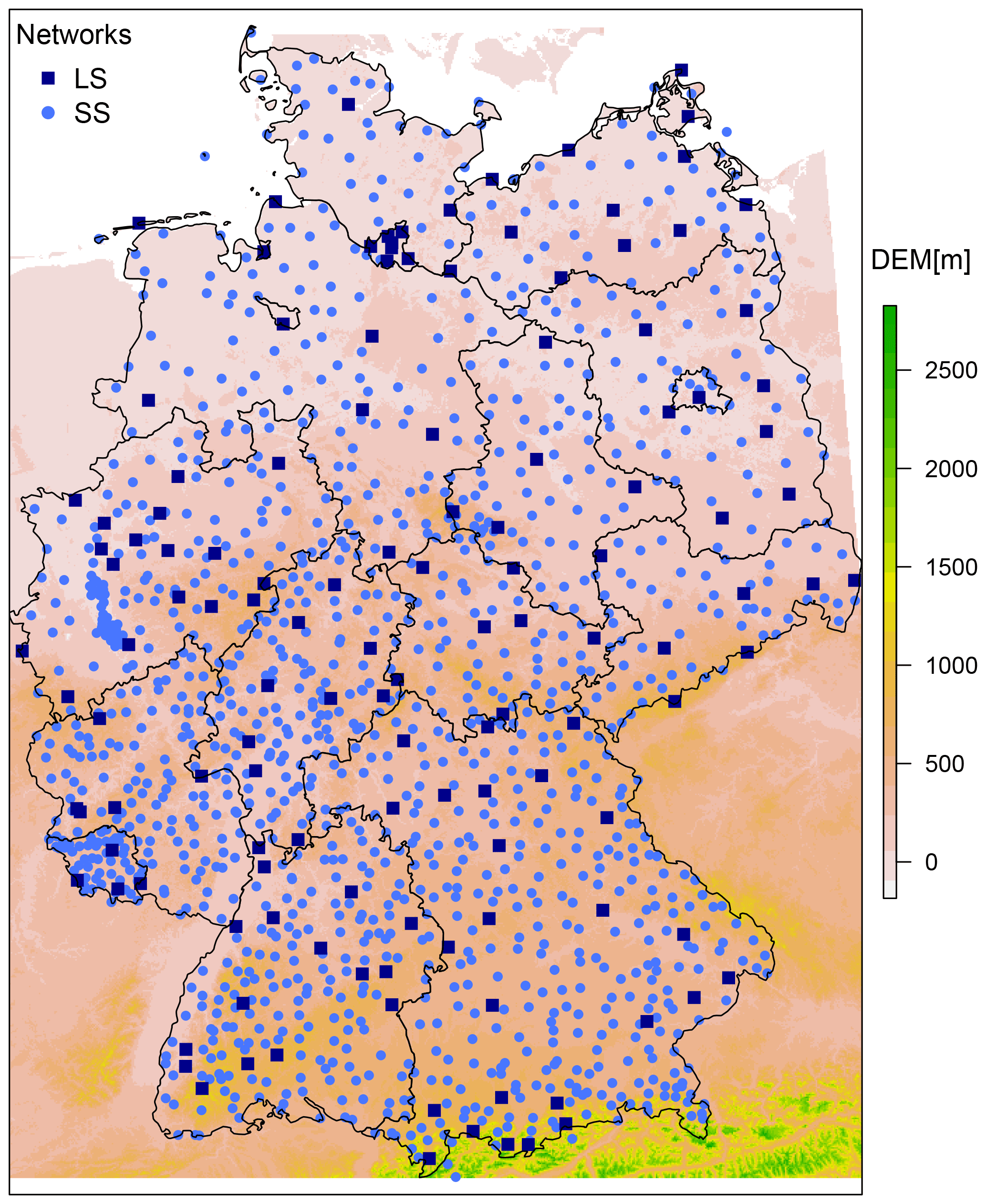
Figure 1 The distribution and location of the two rainfall networks used for the uncertainty analysis of depth–duration–frequency curves in Germany, where LS represents the long and SS the short recording stations. DEM is short for digital elevation model (m) from SRTM (NASA Shuttle Radar Topography Mission, 2013).

2.1 Extreme value analysis

The local rainfall extreme value statistics describing the DDF curves for each station are derived in two steps. First, the intensities of different duration levels are generalised according to the mathematical framework proposed by Koutsoyiannis et al. (1998) also illustrated in Eq. (1):

$$\begin{array}{}\text{(1)}& i=i_d\cdot (d+\mathit{\theta }{)}^{\mathit{\eta }},\end{array}$$

where i is the generalised intensity in millimetres per hour, i_d is the AMS intensity in millimetres per hour at each duration, d is the duration in hours, and θ and η are the Koutsoyiannis parameters optimised for each station. The optimisation of the Koutsoyiannis parameters is done by minimising the Kruskal–Wallis statistic. Second, a generalised extreme value (GEV) distribution is fitted to the generalised intensities through the methods of the L moments (Asquith, 2021). The GEV is described by three parameters: location – μ, scale – σ, and shape – γ (with notation according to Coles, 2001) as given in Eq. (2). For a robust estimation of extreme values with return periods of 100 years, the shape parameter was fixed at 0.1. The decision to fix the shape parameter at 0.1 was made based on the existing literature and previous analysis we conducted on the dataset in Germany. For more information regarding the choice of generalisation or shape parameter, the reader is directed to our previous study (Shehu et al., 2023). Keeping the shape parameter as fixed can be a reasonable choice to reduce the high uncertainty that is associated with the extreme value analysis at single stations. As shown in Shehu et al. (2023), for a return period higher than 20 years, the uncertainty from a free-shape parameter is much higher than the uncertainty from keeping the shape parameter fixed at 0.1, which will cause the interpolation of extreme rainfall to be less certain.

$$\begin{array}{}\text{(2)}& F(x;\mathit{\mu },\mathit{\sigma },\mathit{\gamma })=\exp \mathit{\{}-[\mathrm{1}+\mathit{\gamma }\cdot (x+\mathit{\mu })/\mathit{\sigma }{]}^{-\mathrm{1}/\mathit{\gamma }}\mathit{\}},\mathit{\gamma }=\mathrm{0}.\end{array}$$

Finally, the local statistics of each station are described by five parameters: three from the GEV distribution (μ, σ, γ) and two from the intensity generalisation over all durations (θ, η). Since the shape parameter is fixed at 0.1, only four parameters are regionalised independently from one another using kriging.

2.2 Direct regionalisation (interpolation)

Here a spherical variogram is employed to describe the increment of the variance between any two points of observation situated at a specific distance h, as per Eq. (3). The parameters of the variogram are estimated by the methods of least squares and human supervision.

$$\begin{array}{}\text{(3)}& \begin{array}{rl}& \mathit{\gamma }\left(h\right)=c_{\mathrm{0}}+c\cdot \left({\displaystyle \frac{\mathrm{3}h}{\mathrm{2}a}}-{\displaystyle \frac{h^{\mathrm{3}}}{\mathrm{2}{a}^{\mathrm{3}}}}\right)\mathrm{for}h\le a\mathrm{and}\\ & \mathit{\gamma }\left(h\right)=c\mathrm{for}h=a,\end{array}\end{array}$$

where c₀ is the nugget, c the sill and a the range of the variogram. Once the theoretical variogram is known, it can be used as a basis for regionalising the statistical properties on a 5×5 km grid. The regionalisation (or the interpolation) with kriging is done in two steps, by considering independently the short (SS) and long (LS) recording stations. First, each of the SS parameters is interpolated with ordinary kriging (herein referred to as OK[SS]) based on the theoretical variogram of the SS dataset. Second, each parameter derived from the LS dataset is interpolated with external drift kriging KED[LS|SS] based on the theoretical variogram of the LS dataset, whereas the OK[SS] serves as an external drift. The reason for this two-step procedure is that the short recording stations have an inadequate length for estimating extremes of a high-return period but still provide useful information about the spatial trends. For more information regarding the choice of this spatial regionalisation, the reader is directed to our previous study (Shehu et al., 2023).

2.3 Data transformation

A requirement for the spatial simulations (sequential Gaussian simulation – SGS) is that the target variable to be interpolated (in this case each of the four parameters) should follow a normal distribution. Following the quantile–quantile plot, with sample vs. normal quantiles, illustrated in Fig. 2, it is clear that the datasets (both LS and SS) are not normally distributed, as the extremes (both lower and upper tail) deviate clearly from the normal distribution (the continuous dashed lines). Therefore, in case of a sequential Gaussian simulation (SGS) for assessing the spatial uncertainty, a transformation to normality is required. Deutsch and Journel (1998) propose a normal score transformation based on the empirical probabilities (Weibull plot position) as indicated in Eq. (4).

$$\begin{array}{}\text{(4)}& F(x{)}^{\prime }=\mathrm{1}-{\displaystyle \frac{k}{(n+\mathrm{1})}}\mathrm{and}{x}_{\mathrm{norm}}=G^{-\mathrm{1}}(F\left(x{)}^{\prime }\right),\end{array}$$

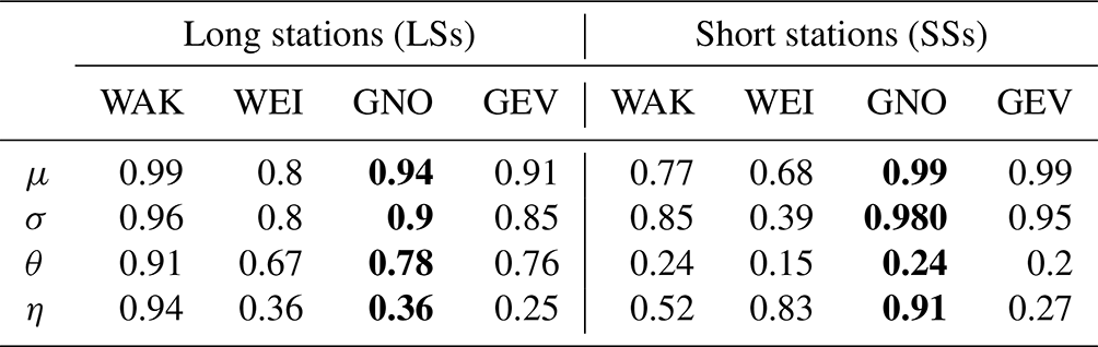
where F(x)^′ is the empirical cumulative distributed function calculated based on the descending rank k of input data x, n is the number of available x observations, G⁻¹ is the inverse function of the Gaussian distribution, and x_norm is the normalised input data. Respectively, a back-transformation algorithm is also available to transform back the dataset from the normal to its original space. However, the back-transformation may be problematic, as the tail behaviour will be underestimated by the normal score and back transformation. An alternative approach to the normal score transformation is the fitting of the theoretical cumulative distribution functions (CDFs) to the original dataset and performing the transformation from the chosen theoretical CDF to the normal one. Here, the problem of the choice for tail extrapolation is substituted with the choice of fitting a theoretical CDF. Through the method of L moments, different theoretical distributions were fitted to the available datasets, for instance, the Wakeby distribution (WAK), the Weibull (WEI), the generalised normal (GNO) and the generalised extreme value (GEV) probability distribution. For more information about the CDF and the fitting of the parameters, the reader is directed to Asquith (2021) and Hosking and Wallis (1997). Afterwards the Cramer–von Mises goodness of fit test (CSöRgő and Faraway, 1996) is performed to test whether or not the observed data belong to the chosen theoretical CDF. The p-value statistics are used to compare the empirical CDF with the theoretical one for each dataset in order to select the most adequate theoretical CDF. The results of the p-value statistics from the Cramer–von Mises test are shown in Table 1, and they reveal that the parameters of the long recording stations (LS) are better described by the WAK distribution, while the parameters of the short recording stations are better described by the GNO distribution. All the parameters, except the θ_[SS], exhibit a very large p value (higher than 0.90). Even though the p value for θ_[SS] is 0.24, the null hypothesis that the theoretical distribution describes in the current dataset can still not be rejected. To keep a consistent choice between the short and the long dataset, the GNO was chosen as the best theoretical distribution for the SS and the second best for LS (shown in bold letters in Table 1).

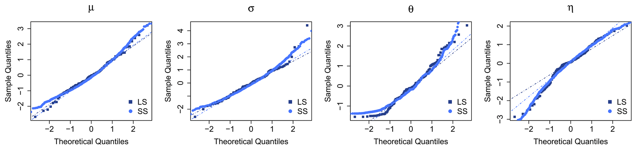
Figure 2 Sample quantiles of the four obtained parameters for both long (LS) and short (SS) datasets in comparison with the theoretical quantiles from the normal distribution. The dashed lines represent the normal quantile lines for a perfect fitting between the sample and the normal quantiles.

Table 1 p values of Cramer–von Mises test to test if the different theoretical distribution fits well to the data. The higher the value, the higher the certainty in accepting the null hypothesis that the chosen CDF correctly describes the data. The p values of the selected CDF for the case study are shown in bold letters.

A comparison of these two transformations, normal score according to Deutsch and Journel (1998) and the quantile–quantile transformation based on fitted theoretical distribution, was performed a priori in cross-validation mode for the SGS runs in ordinary kriging and external drift kriging. The results of such a comparison favoured the quantile–quantile transformation based on fitted theoretical distributions.

2.4 Data bi-normality

An additional precondition to run the SGS and assess the spatial uncertainty is the multivariate normality. However as stated in Deutsch and Journel (1998), the data for checking multivariate normality (the trivariate, quadrivariate and so on) are hardly enough to allow the interference of the corresponding experimental multivariate frequencies. Thus, they suggest that if the bivariate normality conditions are not violated, one can continue with the SGS experiments. Here the bivariate normality is tested by comparing empirical indicator variograms of the normalised parameter sets with the respective ones from a bi-Gaussian random function that shares the same variogram with the normalised parameter sets. First, a theoretical variogram is fitted to the normalised observed variograms from dataset LS and SS (separately). Next the analytical relation given at Deutsch and Journel (1998) linking the covariance C_Y(h) with any normal bivariate CDF value (with mean 0 and standard deviation 1) is illustrated as

$$\begin{array}{}\text{(5)}& \begin{array}{rl}& \mathrm{Prob}\mathit{\left\{}Y\right(u)\le y_{p}Y(u+h)\le y_p\mathit{\}}=\\ & p^{\mathrm{2}}+{\displaystyle \frac{\mathrm{1}}{\mathrm{2}\mathit{\pi }}}\cdot \underset{\mathrm{0}}{\overset{\arcsin C_{\mathit{\gamma }}\left(h\right)}{\int }}\exp \left(-{\displaystyle \frac{{y_p}^{\mathrm{2}}}{\mathrm{1}+\sin \mathit{\theta }}}\right)d\mathit{\theta },\end{array}\end{array}$$

where y_p in the normal p quantile of the normal bivariate CDF, and the C_Y(h) is the correlogram obtained from the normalised LS and SS dataset. For a given threshold y_p, the bivariate probability will be

$$\begin{array}{}\text{(6)}& \begin{array}{rl}& \mathrm{Prob}\mathit{\left\{}Y\right(u)\le y_p,Y(u+h)\le y_p\mathit{\}}=\\ & E\mathit{\left\{}I\right(u;p)\cdot I(u+h;p\left)\mathit{\right\}}=p-{\mathit{\gamma }}_I(h;p),\end{array}\end{array}$$

with I(u;p) equal to 1 for Y(u)≤y_p or equal to 0 if otherwise, and γ_I (h;p) is the indicator variogram for the p quantile (corresponding to threshold y_p) of the normal bivariate CDF. Three thresholds were chosen for the computation of the indicator variograms that correspond to 0.25, 0.5 and 0.75 percentiles. Based on Eq. (6), the generation of the bi-Gaussian functions was performed of each set of data independently (short and long) with the GSLIB package. Lastly, the sample indicator variograms for the three thresholds are computed from the observed normalised datasets. The check consists of comparing the empirical indicator variogram and the theoretical indication variogram from the normal bivariate CDF.

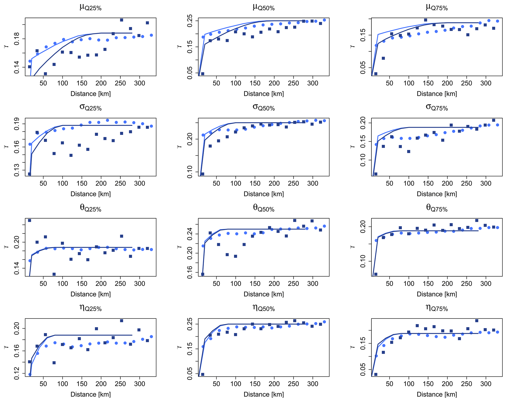
Figure 3 Experimental indicator variograms for the two datasets (SS in light blue, LS in dark blue) for the four parameters and their respective fits of the bi-Gaussian model-derived theoretical curves (shown respectively in solid lines).

The obtained indicator variograms are shown in Fig. 3 for the empirical dataset (in points) and for the bi-Gaussian functions (in solid lines) of the two datasets (short and long). From Fig. 3 it is visible that the bi-Gaussian indicator variograms well described the empirical datasets for most of the cases. For instance, the θ and η parameters show a good agreement for the two types of indicator variograms. For the μ and σ parameters, the agreement is better for the high thresholds than for the low one (0.25 percentile), where mainly the LS dataset differs more with the bi-Gaussian indicator variogram than the SS dataset. To a certain degree this is expected, as the LS dataset is much smaller than the SS dataset. Overall, the bi-Gaussian indicator variograms match well with the empirical ones, and the bivariate normality conditions are not violated. Hence, the SGS can be used for spatial simulation of the parameter sets.

3 Methods for uncertainty estimation

The regionalisation of the four parameters describing the rainfall extreme value statistics is performed using kriging as the best regionalisation method from Shehu et al. (2023). The regionalisation is done primarily with the LS data and using the interpolation of SS parameters as an external drift. In this procedure, there are several sources of uncertainty that one should consider for the overall uncertainty, as illustrated in Fig. 4, which are respectively:

• Sample uncertainty in estimating local extreme value statistics (four parameters is herein referred to as the local uncertainty.

• The uncertainty in the external drift originates from the uncertainty in the estimation of the variogram based on the SS stations, from the uncertainty in the regionalisation of the SS statistics. Here, only the latter is considered, as previous work revealed that this is more relevant than the former.

• The uncertainty in the regionalisation of the LS statistics originates from the estimated variogram from LS stations and the uncertainty of the spatial regionalisation (herein referred to as spatial uncertainty).

Overall, the methodologies to tackle these uncertainties can be categorised in three main groups: the local estimation, the variogram estimation and the spatial simulation (as illustrated in the blocks in Fig. 4). The methodology for uncertainty estimation in each block is discussed accordingly in the following sections.

3.1 Local non-parametric bootstrap

A non-parametric bootstrap approach is implemented in order to quantify the sample uncertainty of the local rainfall extreme value statistics. This means that for each station, the AMS is resampled with replacement for the same length of observations, and the local statistics are then derived based on the methodology explained in Sect. 2.1. This resampling procedure is run 100 times for each location (either LS or SS), and for each time, the parameters describing the local extreme value statistics are calculated. The resampled parameter sets are then used as input for the rest of the regionalisation approach to first investigate the effect of the local uncertainty on the regionalisation output (results shown in Sect. 4.2) or their impact on the overall uncertainty of regionalised DDF curves in Germany (results shown in Sect. 4.3).

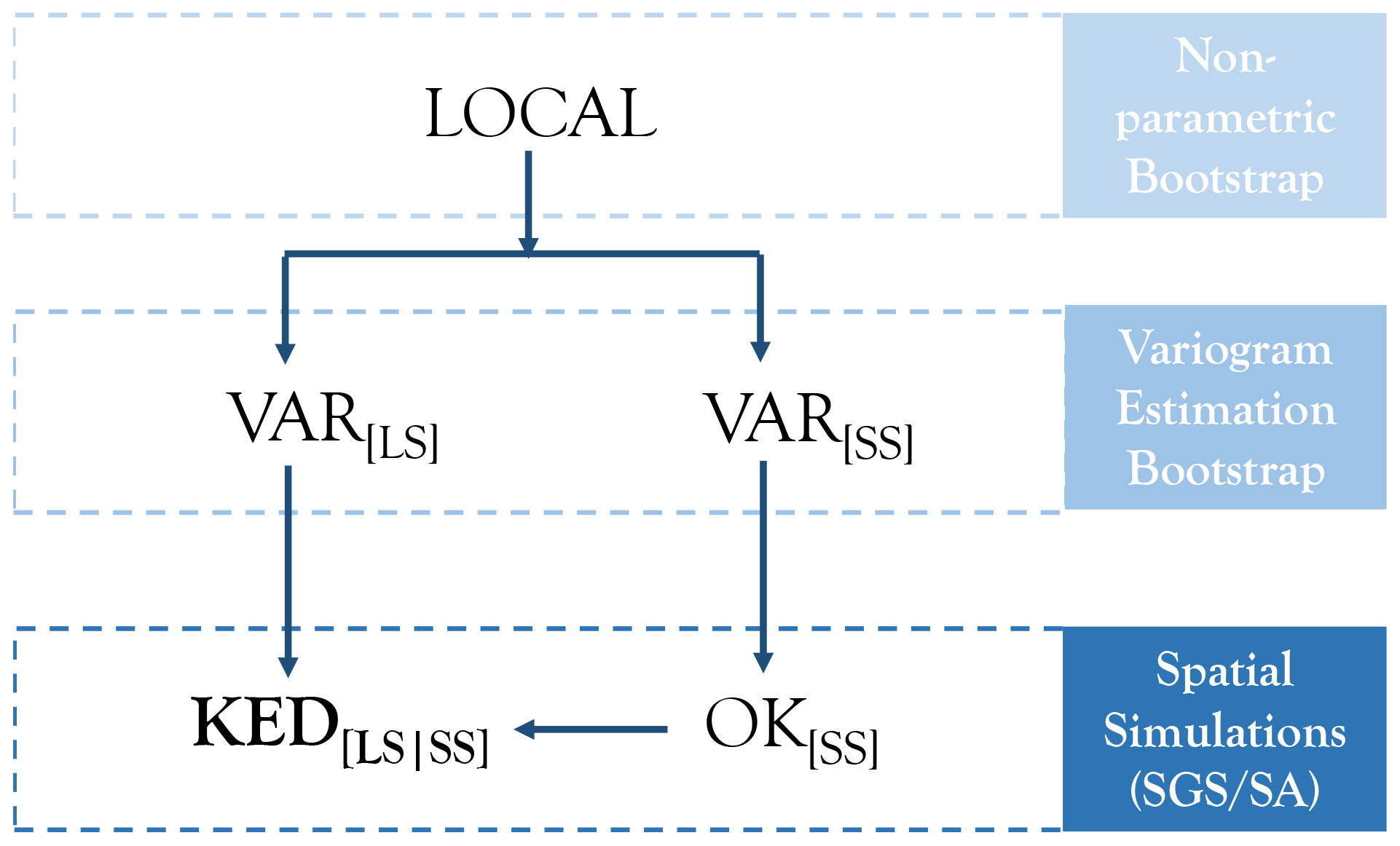
Figure 4 The main uncertainty sources in the regionalisation of the rainfall statistics for Germany for the selected methodology. Arrows indicate the calculation flow, and the blocks on the right represent the three main methodologies to tackle the uncertainty at each component.

3.2 Variogram simulations

A non-parametric bootstrap is implemented in the variogram uncertainty, with the precondition that the spatial dependency between stations is maintained. The whole station dataset (both short and long recordings) is grouped together, from which 133 stations are sampled randomly 100 times. Only 133 values from all the stations were sampled here, to address the uncertainty in computing the variogram from a small dataset that corresponds with the number of the long recording stations that were used to compute the variogram for the KED interpolation. For each of the sample, first the empirical variogram is calculated and then a theoretical spherical one is fitted automatically. Such sampling of variograms is indirectly accounting the low station density and the short observation length for the final interpolation of KED[LS|SS]. The obtained variogram simulations are shown in Fig. 5. For each of the estimated variogram, the kriging interpolation is performed and in the end its effect on the final regionalisation output is discussed in Sect. 4.2.

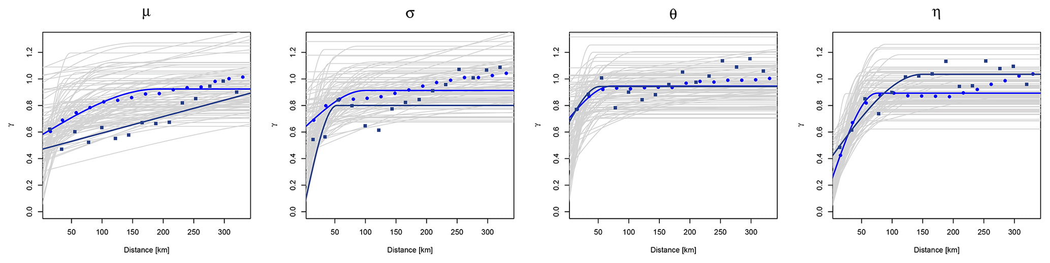
Figure 5 One hundred variogram realisations obtained from bootstrapping (shown in grey lines) the station datasets, the empirical variograms as observed by the normalised LS (in dark blue points) and SS database (in light blue points), and the respective fitted theoretical spherical variograms used for the interpolation.

3.3 Spatial simulations

The uncertainty in the spatial regionalisation is assessed by generating 100 equiprobable realisations of the normalised parameter sets, where each realisation is honouring the global statistics of the parameter (the spatial mean value and the variogram). Here a conditional simulation is performed, where these 100 realisations share not only global statistics but also a set of observed values at certain locations. In other words, for the known locations where there are observations, either the nodes are not resampled (as in the case of simulated annealing) or the nodes are allowed to vary according to the variogram nugget when compared to the observations (as in the case of the sequential Gaussian simulation). The spatial simulations are conditioned to the location of the 133 long recording stations (LS), since they are the main input for the regionalisation and are considered the ground truth.

3.3.1 Sequential Gaussian simulation (SGS)

The sequential Gaussian simulation (SGS) is the most straightforward algorithm for generating such an equiprobable realisation, and it is proven to be more robust than other algorithms (Pebesma and Wesseling, 1998). An overview of this procedure, where a normal continuous variable z(u) is modelled by a Gaussian stationary random function Z(u), is described as follows (Deutsch and Journel, 1998):

1. A random path is defined that visits each node of the Germany grid (at 5×5 km spatial resolution) once. At each node u, fix the neighbouring conditional locations (either SS for OK[SS] and LS for KED[LS|SS]) and their observed values z, and the previously simulated z values at the grid node.

2. Do either ordinary kriging with the normalised short recording stations (OK[SS]) or kriging with external drift with the normalised long recording stations (KED[LS|SS]) using the respective variograms to estimate the global statistics (mean as per Eq. 7, and variance as per Eq. 8) of the conditional cumulative distribution function (CCDF) at the random function Z(u) at the location u.

   $$\begin{array}{}\text{(7)}& {\displaystyle }\mathit{\mu }\left(u\right)=\sum _{i=\mathrm{1}}^n{\mathit{\lambda }}_i\cdot Z\left(u_i\right),\text{(8)}& {\displaystyle }{\mathit{\sigma }}^{\mathrm{2}}\left(u\right)=C\left(\mathrm{0}\right)-\sum _{i=\mathrm{1}}^n{\mathit{\lambda }}_i\cdot C(u-u_i),\end{array}$$

   where λ_i is the weight as estimated by ordinary kriging for OK[SS] and kriging with external drift for KED[LS|SS], Z(u_i) is the conditional value of the target variable at the u_i location, with i corresponding to conditional values in the neighbourhood (within a maximum radius of 300 km and within the range of 12 to 24), C(0) is the variance and C(u−u_i) the covariance of the normalised dataset.

3. Draw randomly a value from this CCDF as z^′(u), and add this simulated value to the conditional dataset.

4. Proceed to the next node until all nodes are simulated.

The gstat package available in R is used to generate such realisations both for the ordinary kriging interpolation of the SS database (OK[SS]) and for the external drift kriging interpolation of the LS database (KED[LS|SS]) (Pebesma, 2004). Note that the spatial simulations are always performed on the normal space (normal transformation of the dataset). For the simulation of the KED[LS|SS], both the input dataset LS and the external drift OK[SS] are also in the normal space. A back-transform to the original space is done after each spatial simulation only for the final product KED[LS|SS].

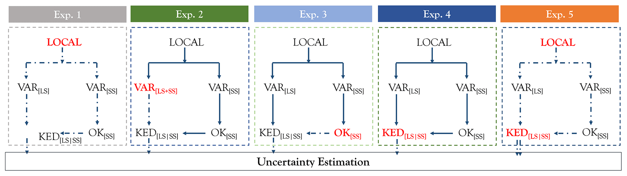
Figure 6 Different experiments run for the propagation of the uncertainty. The bold red letters indicate the source of uncertainty investigated for each experiment and how it propagates throughout the regionalisation procedure (in dashed arrows). The number of arrows in experiment 5 indicate different uncertainty sources combined.

3.3.2 Simulated annealing (SA) simulations

Simulated annealing is an alternative method for generating conditional stochastic images. New images are created by randomly selected values from the observed histograms, such that global statistics like variogram, marginal distribution and correlation to a secondary variable are maintained. Unlike the SGS method, no prior assumption of normality is needed, and hence the observed data (with no prior transformation) can be directly used. An overview of this procedure is found in Deutsch and Journel (1998) and also explained shortly below:

1. An initial image is randomly created by the observed histogram. For nodes where data are observed, the random values are substituted by the observed ones. Thus, the observed values are exactly reproduced. This image matches the observed histogram and conditional data but not the observed variogram.

2. An objective function is calculated, and a conditional simulation is reached when the objective function is as close as possible to zero. For generation of the external drift spatial information (OK[SS]), only the variogram is used as part of the objective function, while for the final parameter estimation (KED[LS|SS]), additionally the correlation with the external drift is preserved.

   $$\begin{array}{}\text{(9)}& \begin{array}{rl}& {\mathrm{OF}}_{\mathrm{OK}\left[\mathrm{SS}\right]}=w_{\mathrm{1}}\cdot \sum _h{\displaystyle \frac{\left[{\mathit{\gamma }}^{\prime }\right(h)-\mathit{\gamma }(h){]}^{\mathrm{2}}}{\mathit{\gamma }(h{)}^{\mathrm{2}}}},\mathrm{and}\\ & {\mathrm{OF}}_{\mathrm{KED}\left[\mathrm{LS}\right|\mathrm{SS}]}=w_{\mathrm{1}}\cdot \sum _h{\displaystyle \frac{{\mathit{\gamma }}^{\prime }\left(h\right)-\mathit{\gamma }\left(h\right){]}^{\mathrm{2}}}{\mathit{\gamma }(h{)}^{\mathrm{2}}}}\\ & +w_{\mathrm{2}}\cdot ({\mathit{\rho }}^{\prime }-\mathit{\rho }{)}^{\mathrm{2}},\end{array}\end{array}$$

   where γ^′(h) is the simulated variogram, γ(h) is the observed variogram, ρ^′ is the simulated correlation, ρ is the observed correlation with the external drift, and w₁ and w₂ are weights for the two components (both equal to 5).

3. If the value of the objective function is not reached, a new image is created by randomly swapping values of pair nodes (not conditioned nodes), and the objective function in recalculated.

4. If the new objective function is better than the previous one (closer to zero), then the swap is accepted; if not, the swap is accepted based on an exponential probability distribution. The parameter of the exponential probability distribution is equal to the temperature in simulated annealing.

   $$\begin{array}{}\text{(10)}& {\mathrm{Prob}}_{\mathrm{accept}}=\left\{\begin{array}{ll}& \mathrm{1},\mathrm{if}{\mathrm{OF}}_{\mathrm{new}}\le {\mathrm{OF}}_{\mathrm{old}}\\ & e^{\frac{({\mathrm{OF}}_{\mathrm{old}}-{\mathrm{OF}}_{\mathrm{new}})}{t}},\mathrm{if}{\mathrm{OF}}_{\mathrm{new}}\le {\mathrm{OF}}_{\mathrm{old}},\end{array}\right.\end{array}$$

   where Prob_accept is the acceptance probability distribution, t is the temperature (which decreases with each iteration), OF_new is the new objective function obtained by swapping a pair of values and OF_old is the previous objective function value. The higher the temperature, the higher the probability to select such unfavourable swaps.

5. Redo steps 3 and 4 until a maximum number of swaps is reached or if a maximum number of accepted swaps is reached. If this is the case, the temperature t is reduced by a multiplicative factor Ω (here as 0.1).

6. Redo steps 3, 4 and 5 until convergence is reached or if the maximum number of possible swaps is reached S times. The simulation is then completed, and the image is frozen.

The GSLIB programme from Deutsch and Journel (1998) was employed to generate 100 random realisation fields for both the external drift and the interpolation. Note two main differences of the SA with SGS: (i) no data transformation and back transformation is required, and (ii) by fixing a seed number, the random path in SGS is same for all the parameters, while for the SA the random path for each parameter depends on how fast the optimum criteria is reached.

3.4 Uncertainty estimation and propagation

Based on several simulations, the uncertainty is evaluated only at the locations on the long recording stations (LS) – in total 133 stations. Different experiments are conducted in order to investigate first how the sources of uncertainty are propagating to the final regionalisation of the four parameters (experiments 1–4), and how the main sources of uncertainty are interacting with each other to produce the total uncertainty (experiment 5). An overview of these experiments and the sources of uncertainty they consider is given in Fig. 6 and in Table 2. Note that in experiment 5, two uncertainty sources are combined: the local uncertainty from the sampling of rainfall extreme value statistics and the spatial uncertainty from KED[LS|SS] simulations. This means that in experiment 5 for each realisation of the local statistics, both variograms of LS and SS are recalculated, the OK[SS] is derived and respectively 100 KED[LS|SS] simulations are generated, concluding thus in a total of 10 000 simulations. The bootstrapping of the variograms (VAR[LS|SS]) is left outside of this experiment, because as it is shown in Sect. 4.2, it does not have a major impact on the regionalisation output. Moreover, as the variograms are re-estimated, different variograms are also modelled, including the variogram uncertainty indirectly. Here only the combination of local and spatial uncertainty at KED[LS|SS] simulations is included as prior work revealed that this produces the highest uncertainty in terms of precision. For each of these experiments, the final regionalisation step of the four parameters (KED[LS|SS]) is run on a cross-validation mode, which means that each of the LS station is left step-wise outside of the database, and the remaining database is used to estimate this LS location. The simulations at the LS stations are then used as a basis for the uncertainty estimation of each parameter separately, and for the final rainfall depth (RD) obtained at specific return periods (T1a, T10a and T100a) and 12 duration intervals (5, 10, 15, 30, 60, 120, 360, 720, 1440, 2880, 7340 and 10 080 min). For each LS location, the uncertainty is estimated based on the experiment simulations using the following criteria:

$$\begin{array}{}\text{(11)}& \begin{array}{rl}& \text{Normalised 95\hspace{0.17em}\% confidence interval width.}\\ & \mathrm{nCI}{\mathrm{95}}_{\mathrm{width}}\left[\mathit{\%}\right]=\mathrm{100}\cdot {\displaystyle \frac{(x_{\mathrm{97.5}\mathit{\%}}-x_{\mathrm{2.5}\mathit{\%}})}{\stackrel{\mathrm{‾}}{x}}},\end{array}\end{array}$$

where x represents the simulations of the target variable at a specific location, x_97.5 % and x_2.5 % are the respective 97.5 % and 2.5 % quantiles of the x simulations, and $\stackrel{\mathrm{‾}}{x}$ is the expected value of x from the simulations of an experiment. The normalised 95 % confidence interval width (nCI95_width) is a measure of spatial simulations precision: the smaller the value, the more robust or precise the estimation method for x is.

$$\begin{array}{}\text{(12)}& \begin{array}{rl}& \text{Average error over all simulations.}\\ & \mathrm{bias}\left[\mathit{\%}\right]=\mathrm{100}\cdot {\displaystyle \frac{{\sum }_{\mathrm{sim}=\mathrm{1}}^{\mathrm{nsim}}\frac{(x_{\mathrm{sim}}-x_{\mathrm{obs}})}{x_{\mathrm{obs}}}}{\mathrm{nsim}}},\end{array}\end{array}$$

where x represents the simulation of the target variable at a specific location from the random simulation sim, x_obs is the local observed target variable at the specific location, and nsim represents the total number of simulations for each experiment. The average error over all the simulations measures the accuracy of the realisation compared to local input data. When rainfall depth (RD) is the target variable, one can go one step further and measure how well the realisations capture the monotonic increase of the RD at different duration intervals for specific return periods, which corresponds to the evaluation criteria in estimating the best regionalisation method for Germany in our previous study (Shehu et al., 2023).

$$\begin{array}{}\text{(13)}& \begin{array}{rl}& \text{Percentage RMSE.}{\mathrm{RMSE}}_{\mathrm{st},\mathrm{T}\left[\mathrm{a}\right]}\left[\mathit{\%}\right]\\ & =\mathrm{100}\cdot {\displaystyle \frac{\sqrt{\frac{\mathrm{1}}{D}{\sum }_{d=\mathrm{1}}^D({\mathrm{RD}}_{\mathrm{regio},d}-{\mathrm{RD}}_{\mathrm{local},d}{)}^{\mathrm{2}}}}{{\stackrel{\mathrm{‾}}{\mathrm{RD}}}_{\mathrm{local}}}},\end{array}\end{array}$$

where T[a] and st are the respective selected return period and LS location, RD_regio corresponds to the regionalised rainfall depth (with KED[LS|SS]), RD_local is the locally derived rainfall depth from the normalised GEV function (from Eqs. 1 and 2), the ${\stackrel{\mathrm{‾}}{\mathrm{RD}}}_{\mathrm{local}}$ is the mean local rainfall depth over all duration levels, and d is an index indicating the iteration from the first to D=12th duration interval. Through Eqs. (12) and (13) and the cross-validation mode, it is possible to compare the performance of the simulations with the direct regionalisation (i.e. interpolation) from Shehu et al. (2023), in order to investigate if the simulation methods are appropriate.

Table 2 The description of the uncertainty propagation for each of the experiments shown in Fig. 6, and the number of realisations considered for each experiment.

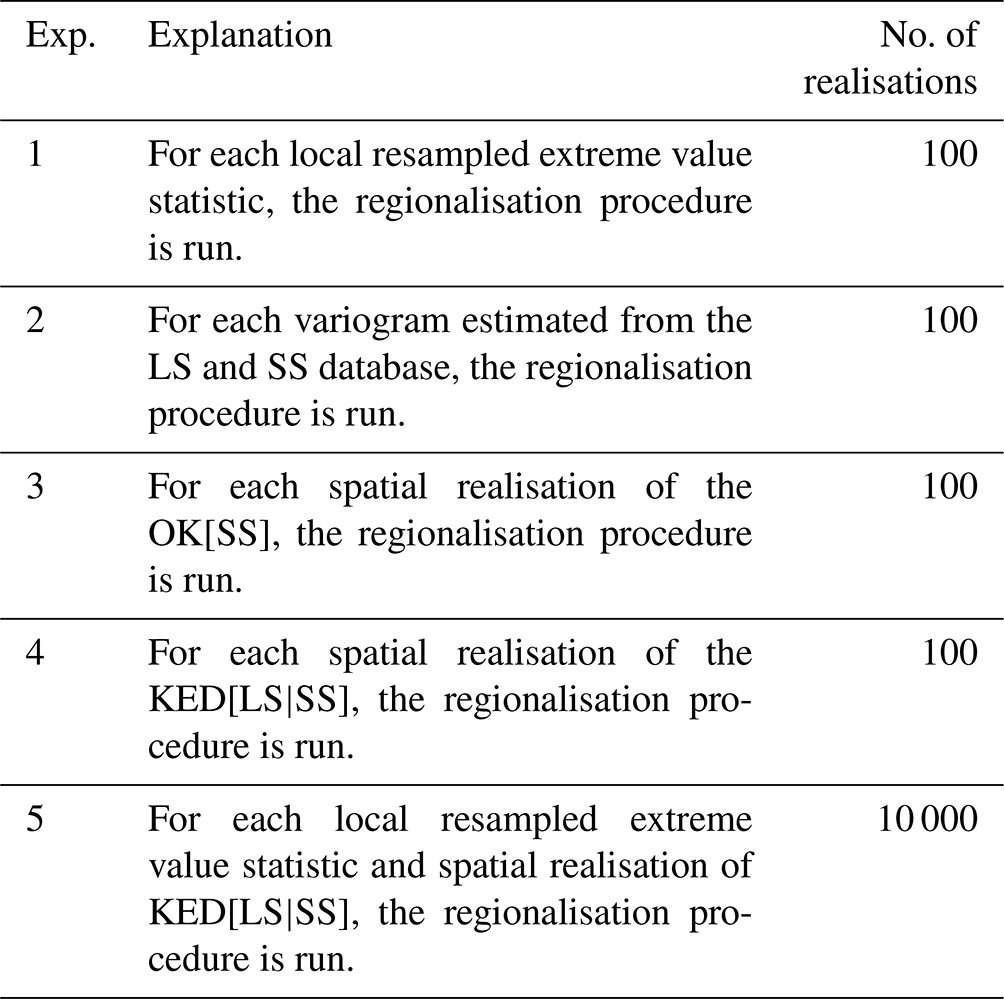
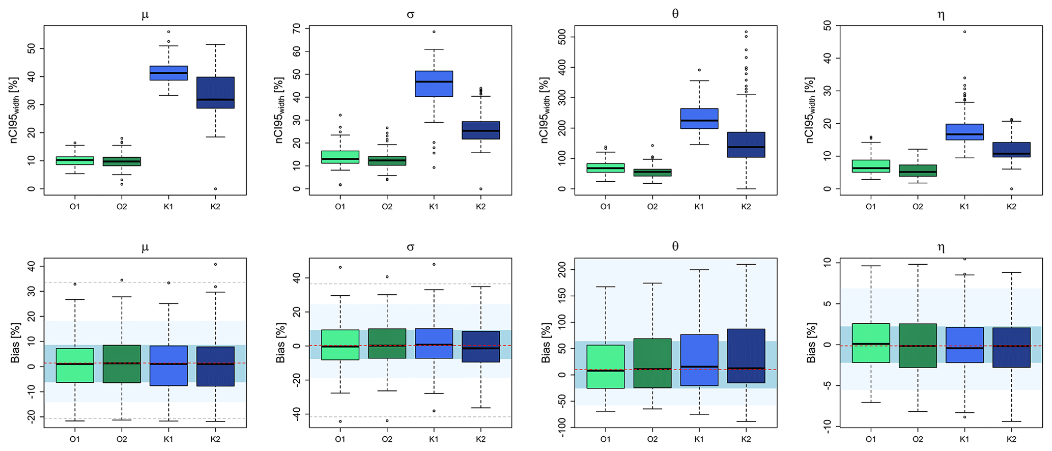
Figure 7 The precision (nCI95_width, %) and accuracy (bias, %) of two different spatial simulations methods (1 – SGS and 2 – SA) for the drift regionalisation (O) and final regionalisation (K) of the four parameters. The boxplots illustrate the performance over the 133 LS locations. The background shades in the lower row illustrate the accuracy of the direct regionalisation (i.e. interpolation) of observed local statistics in a cross-validation mode, where the red dash indicates the median accuracy over all stations, the blue region is the interquartile range (IQR) of all stations, the light blue region is the 95 % and 5 % quantiles, and the dashed grey lines are the maximum and minimum performance over all stations.

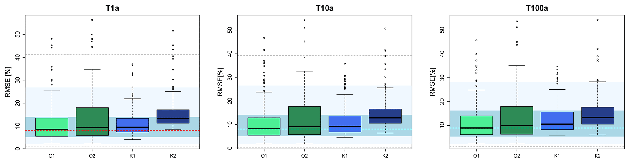
Figure 8 The accuracy (RMSE, %) of two different spatial simulations methods (1 – SGS and 2 – SA) for the drift regionalisation (O) and the final regionalisation (K) of the depth–duration–frequency curves. The boxplots illustrate the median RMSE over the 133 LS locations. The background shades illustrate the accuracy of the direct regionalisation (i.e. interpolation) of observed local statistics in a cross-validation mode, where the red dash indicates the median accuracy over all stations, the blue region is the interquartile range (IQR) of all stations, the light blue region is the 95 % and 5 % quantiles, and the dashed grey lines are the maximum and minimum performance over all stations.

4 Results and discussion

4.1 Comparison of different models in modelling spatial uncertainty

Before analysing the propagation of different uncertainty sources, the best method for computing the spatial uncertainty is investigated. As discussed in Sect. 3.3, two methods are employed for the generation of 100 equiprobable realisations both for the drift information (OK) and the interpolation of the long recording stations with external drift kriging (KED): the sequential Gaussian simulation (SGS) is method 1 and the simulated annealing (SA) is method 2. Figure 7 illustrates the parameter precision (nCI95_width , %) and accuracy (bias, %) of these 100 simulations calculated in cross-validation mode for each of the long recording locations (in total 133) for both methods. Note that the transformation to normality is required only for the SGS and not the SA simulations, as the SA simulations are performed based on observed histograms. The main differences between the two simulation methods are seen in the precision obtained from the 100 realisations (nCI95_width – upper row), where the realisations from the SA approach are more precise than the ones from the SGS approach. The difference in the precision is much higher in the KED[LS|SS] than for the OK[SS] for all the four parameters. In terms of parameter accuracy, both methods have similar performance for both OK[SS] and KED[LS|SS], with SA having slightly higher errors than the SGS and direct regionalisation (i.e. interpolation) performance (particularly for the μ and θ parameters). Overall, it seems that the SA is more precise than the SGS; nevertheless, as the focus is on depth–duration–frequency curves, the methods should also be compared in their ability to estimate the DDF curves. For this purpose, for each cross-validation location, the RMSE (%) was first calculated as per Eq. (13) for each simulation, and then the median over the 100 simulations was obtained. The median RMSE (%) performance for different return periods for both methods is shown in Fig. 8. The median RMSE (%) performance obtained by the SGS method seems to be in accordance with the performance of the direct regionalisation (interpolation) for both OK[SS] and KED[LS|SS]. In contrast, the RMSE (%) performance from the SA simulations is slightly worse than the direct regionalisation for OK[SS] and much worse for the KED[LS|SS] over all return periods (median up to 5 %–8 % higher). Even though the SA produces more precise simulations of parameters, it fails to maintain the interrelationship between the parameters, causing lower accuracy in the DDF estimation. The SGS, on the other hand, keeps the same level of accuracy like the direct regionalisation (interpolation) but with a lower precision. Since the aim is to keep accuracy as in the direct regionalisation (interpolation), SGS was chosen as a more suitable method to model the spatial uncertainty. Also, since the SGS produces a higher range of simulations, the estimated precision, in the end, is more conservative than the SA procedure.

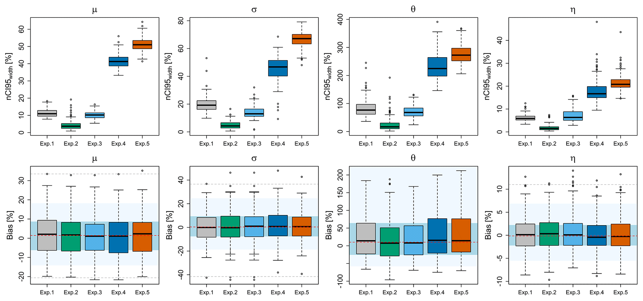
Figure 9 The obtained precision (first row – nCI95_width, %) and accuracy (lower row – bias, %) from propagating the multiple realisations at different components of the regionalisation procedure to the final parameter sets. The background shades in the lower row illustrate the accuracy of the direct regionalisation (i.e. interpolation) of observed local statistics also computed in a cross-validation mode, where the red dash indicates the median accuracy over all stations, the blue region is the interquartile range (IQR) of all stations, the light blue region is the 95 % and 5 % quantiles, and the dashed grey lines are the maximum and minimum performance over all stations.

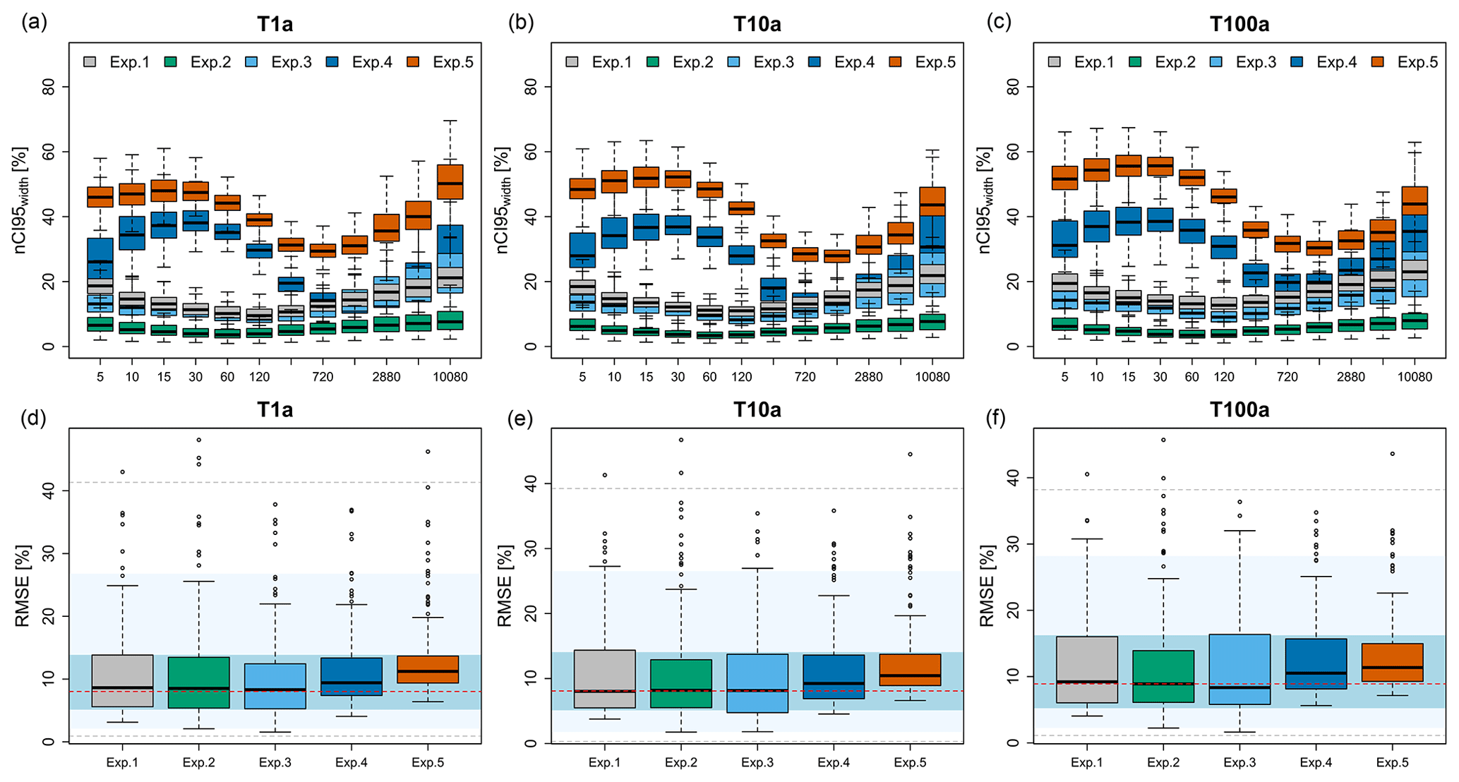
Figure 10 The obtained precision (a–c: nCI95_width, %) and accuracy (d–f: RMSE, %) from propagating the multiple realisations at each component of the regionalisation procedure to the final DDF values. The background shades in (d), (e) and (f) illustrate the accuracy of the direct regionalisation (i.e. interpolation) of observed local statistics also computed in a cross-validation mode, where the red dash indicates the median accuracy over all stations, the blue region is the interquartile range (IQR) of all stations, the light blue region is the 95 % and 5 % quantiles, and the dashed grey lines are the maximum and minimum performance over all stations.

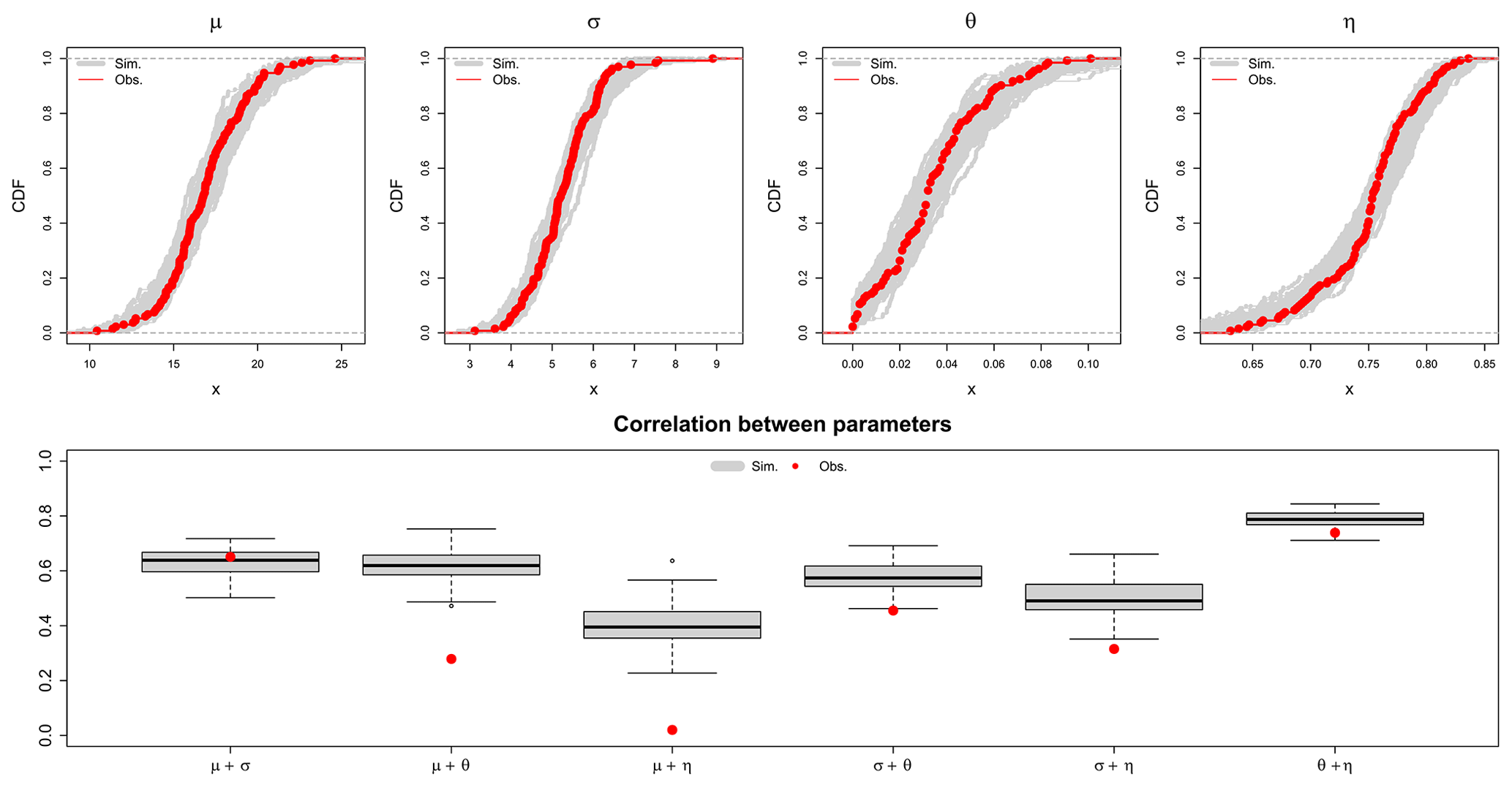
Figure 11 Upper row – empirical CDF simulated from exp. 5 (in grey) and from observed parameter values (in red) over the 133 locations; lower row – observed correlations calculated in space between pairs of LS parameters (shown in red dots) and the respective correlations from 100 KED[LS|SS] simulations (shown in the grey boxplots).

4.2 Effect of different uncertainty components for the estimation of the DDF curves at ungauged locations

Experiments 1 to 4 were conducted in order to investigate the uncertainty propagation from each component of regionalisation to the final parameter and DDF values, while Experiment 5 considers a propagation of the two main uncertainty sources interacting in the final regionalisation of the extremes. The parameter uncertainty is calculated from the number of simulations given in Table 2 for each experiment and is illustrated in Fig. 9, where the upper rows represent the precision (nCI95_width, %), while the lower rows are the accuracy (bias, %) of estimated parameters in cross-validation mode. Figure 10 illustrates the DDF uncertainty at duration levels from 5 min up to 7 d for three return periods 1, 10 and 100 years: precision (nCI95_width, %) shown in the upper row and accuracy (RMSE, %) in the lower row. The accuracy of the simulations is compared with the direct regionalisation (i.e. interpolation) of the observed parameter sets (see caption for more details). It is worth mentioning that the difference between the different component simulations (experiments 1 to 4) is visible only at the precision of the simulations and not at the accuracy. As illustrated by Fig. 9 (lower row) and Fig. 10 (lower row), the accuracy in estimating the parameters (bias, %) and the DDF values (RMSE, %) does not change considerably from one experiment to the other. Also, when comparing the boxplots with the performance obtained from the direct regionalisation (interpolation – shown with the background colours), the same accuracy more or less is observed. Therefore, the analysis will be focused on the variation of precision (nCI95_width, %) according to different sources of uncertainty. Regarding the parameter uncertainty as shown in Fig. 9, the spatial KED[LS|SS] simulations (exp. 4) represent the highest source of uncertainties for all the parameters: the nCI95_width, %, ranges from 18 % for the η parameter, between 40 %–50 % for the two GEV parameters μ and σ, and up to 250 % for the θ parameter. The parameters vary greatly in space, and that is why when sampling from space (spatial simulations), the prediction intervals are higher than for the bootstrapping case (or the other cases). For all the parameters, the nCI95_width of the KED[LS|SS] simulations is at least 3 times higher than the nCI95_width of the other uncertainty sources, concluding that the spatial simulations add the biggest uncertainty to the regionalisation. Second to the KED[LS|SS] simulations is the resampling of local statistics (exp. 1) and the OK[SS] simulations (exp. 3), which seem to produce similar levels of nCI95_width for most parameters ranging from 10 % for the location μ, 90 % for the θ and only 8 % for the η parameter. Only for the scale GEV parameter (σ) is the nCI95_width from the local statistics resampling higher (≈20 %) than the one from OK[SS] (≈15 %). It is interesting to see that the obtained nCI95_width from the variogram bootstrapping (exp. 2) is lower than 5 % for almost all parameters (except the θ parameter which is lower than 20 %). This suggests that the variability between interpolated fields with different variograms reproduces very similar spatial parameters, even though the variograms differ greatly in terms of nugget, sill and range (see Fig. 5). The same behaviour is also seen in estimated DDF curves for different return periods (Fig. 10 – upper row), where the variability as exhibited by the variogram bootstrapping (exp. 2) is very low (less than 10 %) compared to the other simulations and is also constant over the duration levels. On the other hand, the simulations from both local resampling (exp. 1) and OK[SS] simulations (exp. 2) exhibit similar patterns of nCI95_width for the selected DDF curves (Fig. 10 – upper row). Unlike the nCI95_width exhibited in the parameter simulations, here the difference between these two components is more visible, as the nCI95_width produced by the local resampling (exp. 1) is 1 %–5 % higher than the one produced by the OK[SS] simulations (exp. 3). As also seen in Fig. 10 (upper row), the nCI95_width from the KED[LS|SS] (exp. 4) is the highest compared to the other components, emphasising that the spatial uncertainty of the KED[LS|SS] is the main source of uncertainty when regionalising the DDF curves. Also, unlike the other types of uncertainties (exp. 1 to 3), the spatial uncertainty from the KED[LS|SS] depends greatly on the duration level, with nCI95_width values of short-duration intervals (from 5 min up to 2 h) being considerably higher than the other experiments (reaching values of 40 % on average). Moreover, exp. 4 boxplots are much wider than exp. 1 to 3, suggesting that the spatial uncertainty is highly dependent on the location. The high uncertainty values in terms of precision for exp. 4 come with the cost of slightly increased error in RMSE (Fig. 10 -lower row), where the median RMSE values are 1 %–2 % higher than those of the direct regionalisation but still within the interquartile range (IQR) of the direct regionalisation performance. So far, experiments 1 to 4 have considered the propagation of singular uncertainty sources to the final regionalisation of parameters and DDF curves in Germany. Experiment 5 considers a propagation of the two main uncertainty sources interacting together in the final regionalisation of the DDF curves. As stated before, the most important sources are the local estimation of rainfall extreme statistics and the spatial uncertainty in regionalisation (KED[LS|SS]). As the variogram and the external drift is calculated for each local resampling dataset, the uncertainty of variogram and external drift is already included in the propagation of uncertainty from local resampling to spatial simulations. For each of the two components, 100 realisations are run, resulting in a total of 10 000 simulations. Overall, the final and total uncertainty from exp. 5 follows a similar pattern to the uncertainty from KED[LS|SS] simulations, but due to the local uncertainties, it manifests higher values of nCI95_width and RMSE (as seen in Figs. 9 and 10). The variation of the total nCI95_width for almost all parameters is 10 %–20 % higher than those of exp. 4, with the GEV parameters reaching values of 50 % (μ) to 70 % (σ), the θ parameter up to 270 % and the η parameter up to 20 %. Consequently, the variation of the total nCI95_width over the duration levels is between 35 %–50 % for return periods 1 and 10 years and between 40 %–80 % for return period of 100 years. As with the KED[LS|SS] simulations (exp. 4), the durations shorter than 120 min and the ones longer than 3 d exhibit higher nCI95_width values, with the durations from 6–48 h having the highest precision (lowest nCI95_width values). Another property seen from experiment 5 is that the variation in space (the wideness of boxplots) is narrower than in exp. 4 for most of the durations, suggesting that the final spatial uncertainty is more constant in space (inheriting a property from local uncertainty – exp. 1). In terms of accuracy, the RMSE (%) has been increased on average with 3 % for 1-year return period, and to 4 %–5 % for 10–100-year return periods, differing slightly from the direct regionalisation (i.e. interpolation) performance but still within the interquartile range (IQR) of the direct regionalisation. Some outliers are present in the accuracy plot (lower row in Fig. 10); however, except for one location, these outliers are within the maximum RMSE manifested by the direct regionalisation. The behaviour of these outliers emerges both from parameter outliers and from looking at the quantiles. They are present in locations where parameters are considerably different from the neighbour long observations (as in the case of singular stations in the Black Forest or the Alps), or where a parameter outlier is located (as in the case of Münster where a very rare extreme event in 2014 causes a high value for the scale σ parameter) and is not geographically clustered. Since the median of the simulations from experiment 5 increases slightly the RMSE (%) but still within the IQR of the direct regionalisation, the simulations can be used to quantify the total uncertainty range for the regionalisation of the depth–duration–frequency curves. In this context, the nCI95_width (%) values in Fig. 10 can be divided by 2, to show the tolerance range above or below the predicted values at each node from the direct regionalisation. For instance, if at a specific location, for a duration of 5 min and return period of 100 years, the simulated nCI95_width (%) is 40 %, this means that the regionalised rainfall depth at this location varies with ±20 % of its mean value. A parabolic relationship is visible for experiments 1–3, with lower nCI95_width values at the mid-duration levels (1 and 2 h) and increasing values at lower and longer durations. This parabolic behaviour over the different duration levels is attributed to the Koutsoyiannis framework for generalising the intensities over all durations by the two parameters θ and η. A particular behaviour is the variation of the nCI95_width over the DDF values from the KED[LS|SS] simulations (exp. 4), which is also inherited at the final uncertainty computation (exp. 5). The behaviour exhibited by KED[LS|SS] simulations does not follow a parabolic function as in exp. 1, exp. 2 and exp. 3 but more a sinusoidal one. This can be attributed to two main reasons: (1) the effect of the Koutsoyiannis parameters on different durations and (2) the spatial simulations of the SGS algorithm following the transformation to normality.

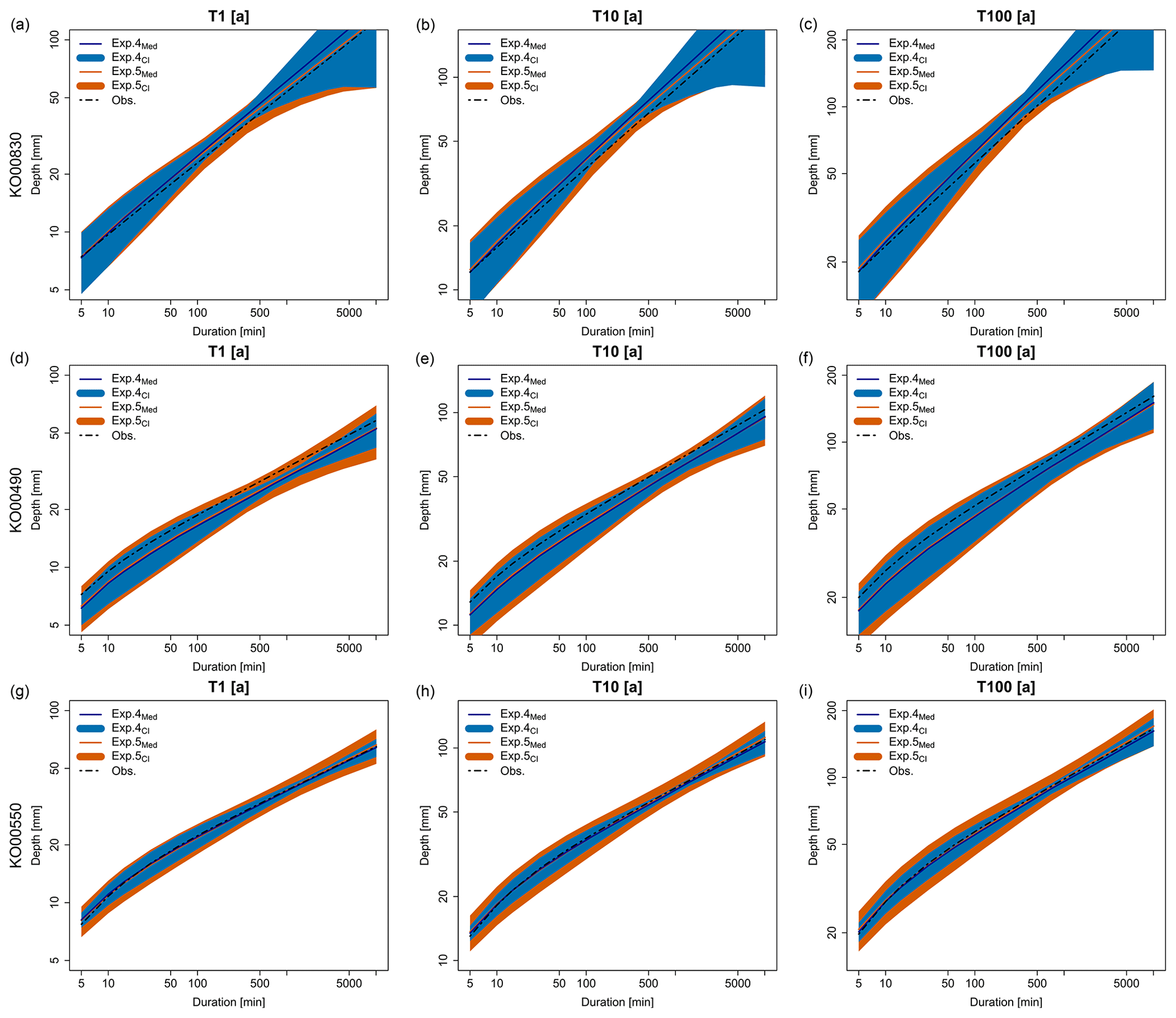
Figure 12 Examples of DDF estimates from observed data and predicted by simulations of exps. 4 and 5 in cross-validation mode as median over all simulations and as 95 % tolerance ranges from all simulations. (a), (b) and (c) for return period T=1 years; (d), (e) and (f) for T=10 years; and (g), (h) and (i) for return period T=100 years. Three stations are shown here are K000830 located in the German Alps, KO00490 location in Lower Saxony and KO00550 located in the Black Forest.

Figure 11 (upper row) illustrates the observed empirical and simulated CDF from exp. 4 for each parameter extracted from the LS dataset. Overall, the simulated CDFs agree well with the observed CDFs; however, the tails might diverge slightly. This is particularly true for the lower tail of the θ and η parameters and the upper tail of the σ parameter. This occurs as the transformation is done on a continuous CDF, a GNO is first fitted to the data, and based on the GNO CDF, the transformation is performed. Nevertheless, this is not negative, as like this, values outside the observed range are simulated; hence, higher or lower values can be simulated as well. As stated in Marra et al. (2019a), the rainfall stations will not capture the maximum intensities of a storm, and thus, it is almost certain that they do not represent the high possible intensities. Therefore, generating higher or lower parameter values than observed is crucial in the generation of stochastic simulations. Figure 11 (lower row) illustrates the correlation between pairs of LS parameters (shown in red dots) and the corresponding correlations obtained from the 100 KED[LS|SS] simulations run in the cross-validation mode. For the μ–σ pair, the observed correlation is well captured, as it coincides with the median of the simulations. To a certain degree, this is also true for the θ–η pair. The main differences are in the relationships between the GEV and Koutsoyiannis parameters, where the simulated correlation is much higher than observed. In particular, the correlation between μ, σ and θ is higher than the correlation between μ, σ and η. This explains why the precision of the KED[LS|SS] has a sinusoidal behaviour. The fluctuation of the θ parameter affects the uncertainty of the short durations (mainly from 5 to 60 min), while the fluctuation of the η parameter affects the uncertainty at short (5–30 min) and very long durations (12 h to 7 d). Since the θ parameter is highly correlated with the μ and σ parameters, its fluctuations will result in a smaller uncertainty than the η fluctuations, resulting in a slight increase of precision between the duration of 5–30 min. In KOSTRA2010R, which provides design storms for Germany, no objective uncertainty analysis was performed to give the confidence intervals between 10 %–20 % and hence should not be directly compared with the objective uncertainty estimation performed here. The total uncertainty considered here (from exp. 5) depends not only on the return period but also on the duration level. The results from Fig. 10 can be used to determine the tolerance above (+) and below (−) the median for the 95 % confidence level. This will result in a median uncertainty range from ± 15 %–25 % for low-return periods (lower than 10 years) and from ± 20 %–40 % for high-return periods (higher than 10 years). Moreover, the short durations (5 min to 2 h) are in general 20 %–30 % more uncertain than the longer durations (6 h–1 d). The behaviour exhibited here is also in accordance with other studies (for instance Marra et al., 2017) where the shorter-duration intervals are more uncertain than the ones of 1 d. In this section, we compare the uncertainty estimation from two experiments 4 and 5, to see how they are distinguished from one another. Uncertainty from experiment 1 is left out, not only to keep the graphics simple for visualisation, but also because it is much narrower than for the other two experiments and it is enclosed in exp. 5. Examples of depth–duration–frequency curves and tolerance ranges for three stations and three return periods (T=1, 10 and 100 years) are illustrated in Fig. 12 for three methods: only spatial KED[LS|SS] simulations (from exp. 4) in blue, local and spatial simulations (from exp. 5) in orange, and local derived DDF curves in the dashed black line. Note that the results shown here are also obtained in cross-validation mode, which of course overestimates the overall uncertainty at these locations. The first station KO00830 is located in Oberstdorf (a town in the Allgäu Alps of Germany), the second KO000490 in Soltau, Lower Saxony, and the third KO00550 in Emmendingen in the Black Forest region. These three stations were selected as representative of different regions and behaviours. Over all the stations, the tolerance range computed by the two experiments is wider at short-duration intervals. This is true for all return periods, but the tolerance ranges get wider with the increasing return period. As seen from first row, the expected rainfall depth in the German Alps is much higher than the two others, followed by the station in Soltau and the one in the Black Forest. Because of the low station density in the Alp region, the tolerance range is wider than in other locations. Overall the two products are similar to each other, with the main difference present mainly at the durations from 6 to 12 h, where exp. 5 exhibits wider tolerance ranges. Regarding the median estimation of DDF from both experiments, the main difference is seen in the Alps, where exp. 5 agrees better with the observed values. Lastly, we recommend quantifying the uncertainty based on exp. 5, since the tolerance ranges better represent the duration levels from 6–12 h and its median matches better with the observation.

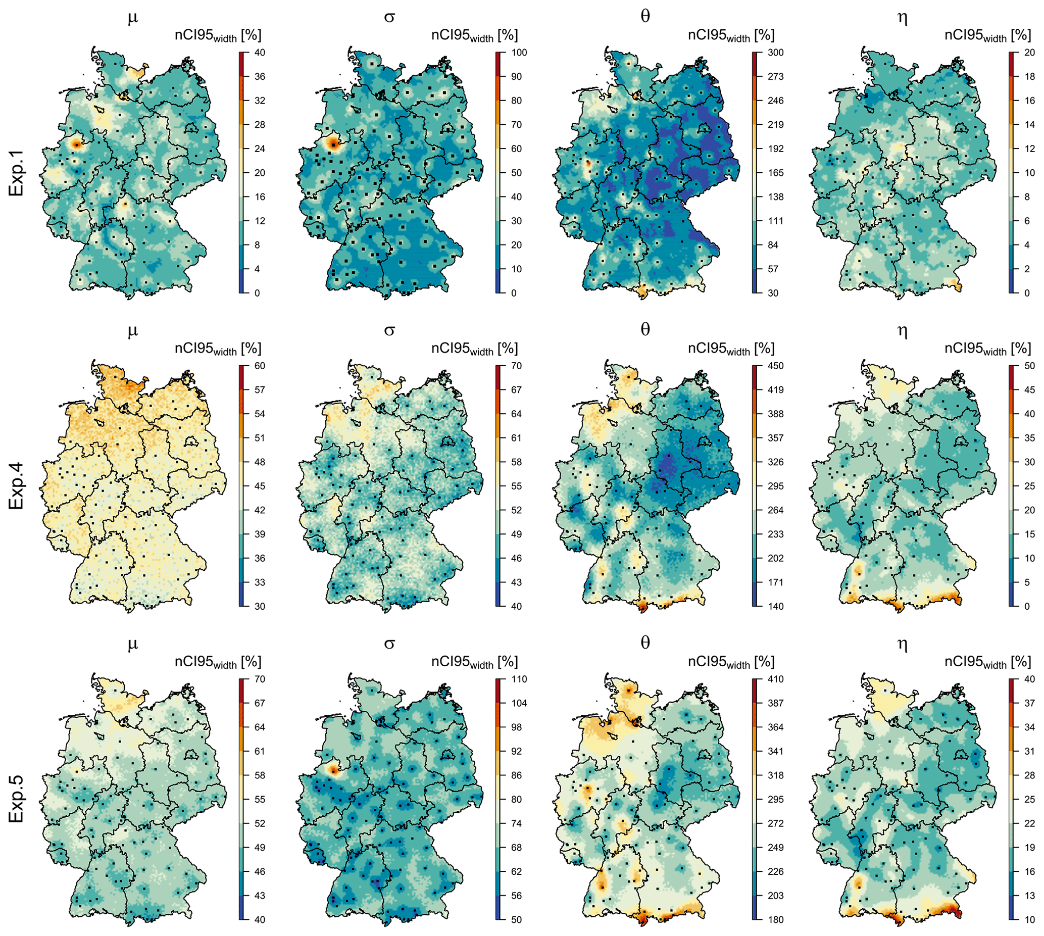
Figure 13 The precision (nCI95_width, %) in estimating the four parameters for the whole of Germany with all available data for two experiments: upper row – results obtained from the propagation of 100 local resampled data to the final regionalisation (exp. 1), middle row – results obtained from 100 spatial simulations of KED[LS|SS] (exp. 4), and lower row – results obtained from 10 000 local resampling and spatial simulations of KED[LS|SS] (exp. 5). The black squares indicate the locations of LS, while the black lines illustrate the boundaries of German federal states. Note that the ranges for the legend colourschange for each experiment in order to emphasise the spatial structure of each experiment.

4.3 Spatial structure of uncertainty for the whole of Germany

Spatial maps of precision were generated for three experiments (exps. 1, 4 and 5), by using the whole dataset, in order to investigate the spatial distribution of the precision when generating the DDF curves for Germany. The precision in terms of nCI95_width, %, for the four parameters describing the extreme value statistics is given in Fig. 13. It can be seen that the different sources of uncertainties exhibit different precision over Germany. For instance, a propagation of the local uncertainty (exp. 1 showed at the first row) causes less precision at observed locations (shown in black) than at the unobserved location. This is because the resampling of the target network (LS) proves more uncertainty than resampling the external drift network (SS). Therefore, uncertainty estimated from exp. 1 is not enough to capture the spatial structure of the uncertainties. On the other hand, exp. 4 shows a clear spatial structure for uncertainty (mainly for three parameters σ, θ and η), with the north-west and south of Germany having higher uncertainty ranges. This follows the precipitation regime and the station density in Germany; the south parts record higher precipitation amounts because of the German Alps (so it is a region with clearly different behaviour than the rest of Germany), while the north-west has a lower station density for both the LS and SS datasets in comparison with the rest of Germany. The uncertainty range at two parameters μ and σ increases with 30 %–40 % for the whole of Germany when combining the local and spatial uncertainty (exp. 5) in comparison to only spatial uncertainty (exp. 4). The uncertainty at the parameters θ and η remains more or less at similar levels, with similar spatial patterns. Thus, including the local uncertainty mainly influences the parameters of the GEV distributions. It is interesting to see in exp. 5 that, at the location of the long recording stations (shown in black squares), the uncertainty of the parameters μ and σ is much lower than for the rest of the regions. This is an expected behaviour, as observed locations should be more certain than unobserved ones, and as the station density decreases, the uncertainty increases. This behaviour, not seen in other experiments, seems to be captured quite well by exp. 5. This is particularly true for the GEV parameters, while the Koutsoyiannis parameters show an additional spatial variability of uncertainty that follows the main elevation features in Germany (represented by the external drift), with the north-west and south of Germany having higher uncertainty ranges. Another interesting point is the high uncertainty associated with the σ parameter by exp. 5 in Münster (shown in a red circle), which is also visible in exp. 1. The high uncertainty of the scale parameters comes mainly from the local resampling bootstrap. As discussed in Shehu et al. (2023), a very rare extreme event was recorded in 2014 in Münster, which affects the extreme value analysis considerably. Thus, the integration of the local uncertainty becomes mandatory to estimate the uncertainty when including these rare events (with a very high-return period) in the estimation of DDF curves for design purposes.

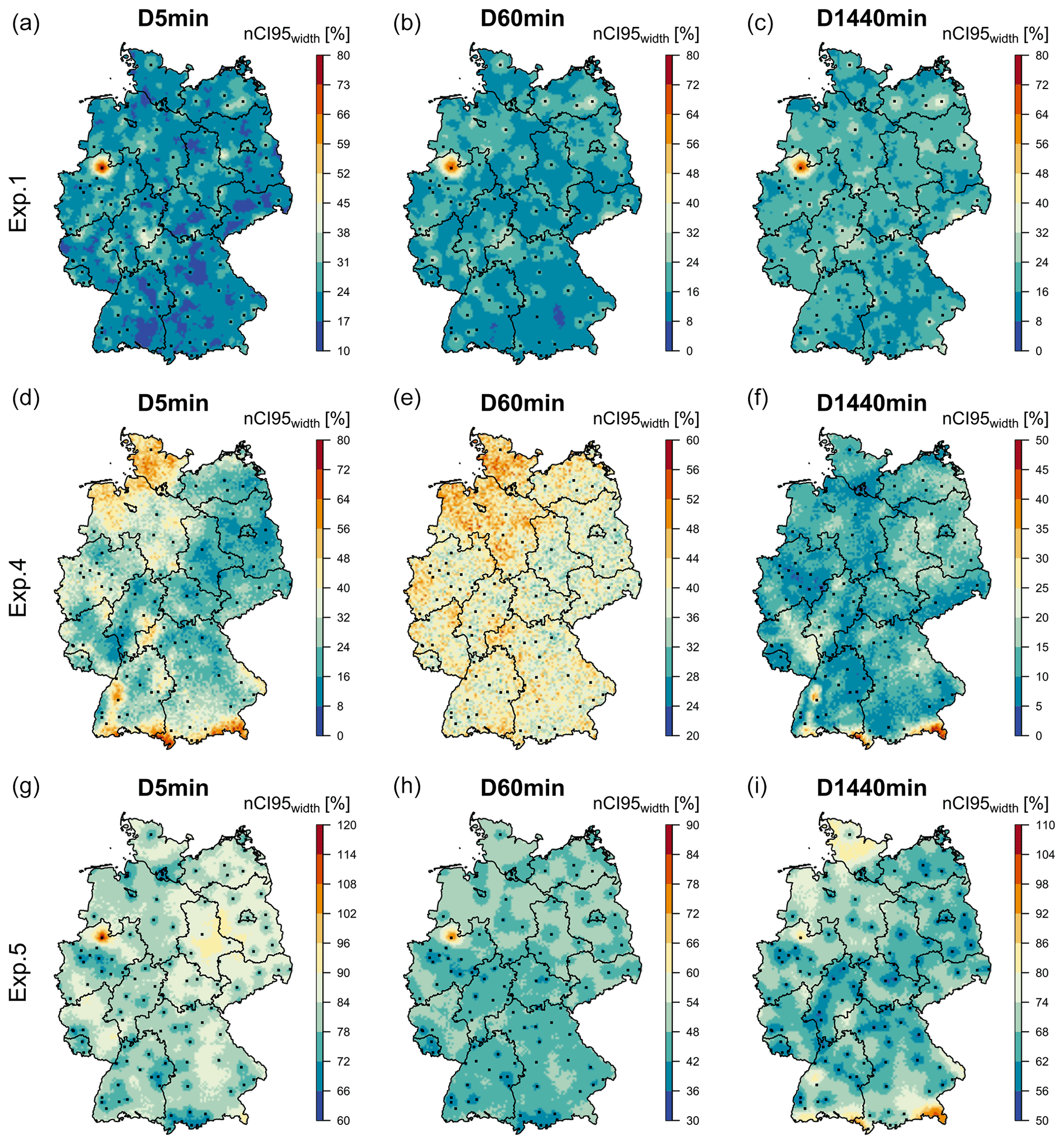
Figure 14 The precision (nCI95_width, %) in estimation rainfall depth at different durations and the 100-year return period for the whole of Germany with all available data for three experiments: (a–c) results obtained from the propagation of 100 local resampled data to the final regionalisation (exp. 1), (d–f) results obtained from 100 spatial simulations of KED[LS|SS] (exp. 4), (g–i) results obtained from 10 000 local resampling and spatial simulations of KED[LS|SS] (exp. 5). The black squares indicate the locations of LS, while the black lines illustrate the boundaries of German federal states. Note that the ranges for the legend colours change for each experiment in order to emphasise the spatial structure of each experiment.

Figure 14 illustrates the spatial distribution of uncertainty (computed here in terms of the precision of nCI95_width, %) for the durations 5 min, 1 h, 1 d and return period of 100 years: upper row – only from local uncertainty (exp. 1), second row – only from spatial uncertainty (exp. 4) and lower row – from both local and spatial uncertainty (exp. 5). The uncertainty ranges exhibited by exp. 1 (only considering the local uncertainty) are very similar throughout all three durations and maintain similar spatial structure as with the parameter uncertainty in Fig. 13. Here, the difference between observed and unobserved locations is small, and, following the parameter precision, the observed locations have higher uncertainty that the unobserved ones (on average 15 %–20 % higher nCI95_width values). In exp. 4, there is a clear difference between the uncertainties of different durations, where the uncertainty of very short and very long durations (5 min and 1 d) is governed by the spatial structure of θ and η parameters. The uncertainty of 1 h durations is more or less uniformly distributed, but with the north-west region exhibiting higher uncertainties than the rest of Germany. In exp. 5, the uncertainty for 5 min durations has been increased considerably when including the local uncertainty (from 20 %–55 % in exp. 4 to 80 %–100 %). The uncertainty of 1 h durations exhibits similar patterns but is increased slightly from 45 % to 55 % in exp. 5. For 1 d duration, the uncertainty ranges are also increased by exp. 5, with values higher at the southern part of Germany (where the German Alps are located) and at the northern part of Germany near to the North Sea. The extreme event at Münster influences the uncertainty of all durations but has a higher impact of short durations. Based on such propagation of uncertainty, tolerance ranges between ± 30 %–60 % should be expected in Germany for 5 min duration intervals, ± 15 %–45 % for 1 h durations and ± 20 %–50 % for 1 d durations. Overall, the combination of local resampling with geostatistical spatial simulations provides the best method for the assessment of uncertainty in regionalisation DDF curves in Germany. First, and most importantly, the precision of these curves is higher at the location of long recording stations and decreases in ungauged locations according to the distance from the long observations and the density of the observations in the vicinity.

5 Conclusions

In Shehu et al. (2023), a regionalisation based on external drift kriging was employed to calculate depth–duration–frequency (DDF) curves in Germany. Based on these results, an uncertainty analysis was conducted here to estimate the precision of the obtained regionalised DDF curves in Germany. For this purpose, many simulations were performed at the main components of the regionalisation procedure: local estimation of the extreme statistics (by non-parametric bootstrapping), spatial dependency (by variogram bootstrapping) of short and long recording stations statistics, the external drift information (by sequential Gaussian simulations) and the interpolation (also with sequential Gaussian simulations). Four different experiments were run in order to estimate how the uncertainty at each component propagates to the final regionalisation of the DDF curves, and a last experiment was performed by combing the uncertainty of the two main components in order to assess the total uncertainty. The uncertainty, in terms of precision, was evaluated at each long recording station location (in cross-validation mode) based on the obtained 95 % confidence interval from different simulations. The conclusions from this investigation are summarised below:

• A comparison with simulated annealing showed that the SGS is better suited for the study at hand, as it shows higher accuracy by capturing better the interrelationship between the parameters (despite of the data transformation). Further works may include a new SA algorithm that models the four parameters together in space in order to keep the interrelationship between them. A future improved SA algorithm may have the potential to decrease the overall uncertainty ranges of DDF curves further on.

• The uncertainty from the variograms that describes the spatial dependencies within the short and long observation datasets does not seem to influence much the final regionalisation of parameters and hence the estimation of the DDF curves. Therefore, it was neglected for the total uncertainty propagation. On the other hand, the uncertainty from the regionalisation of the long observations is the biggest source of uncertainty, followed by the local estimation of extremes and by the drift estimation from short observation. A bootstrapping technique that combines the local estimation of extremes with different spatial simulations of the long observations provided the highest uncertainty and was used to quantify the total uncertainty.

• The total uncertainty obtained here mainly follows the behaviour of the spatial uncertainty but is slightly higher, as it is influenced by the local uncertainty. However, unlike the spatial uncertainty, the total uncertainty is influenced by the very rare extreme events and also considers them for the computation of tolerance ranges. Moreover, by combining local resampling with spatial simulations, the modelled uncertainty exhibits valid behaviour: at observed locations, the precision is higher, and it decreases at unobserved locations according to the distance from the observed and the density of the observed locations in the vicinity. For very short and very long durations, uncertainty ranges are also dependent on different climatological regions in Germany.

• From 10 000 simulations, it is concluded that the durations shorter than 2 h exhibit a larger uncertainty than longer durations, which of course is increasing with the return period considered. Depending on the location and duration, tolerance ranges from ± 10 %–30 % for low-return periods (lower than 10 years) and from ± 15 %–60 % for high-return periods (higher than 10 years) should be expected.

• For the proposed methodology, the uncertainty variation in space (for most locations) seems to be smaller (≈ 10 %–20 %) than the variation across different durations (up to 30 %). On the other hand, the uncertainty variation due to the return periods is low, approximately 5 % to 10 %. The only exception is at Münster, where a very rare extreme event has been observed and causes high uncertainty ranges for the extreme values in the vicinity. Events such at the one in Münster influence the DDF curves considerably, and hence more research should be done in order to investigate how to treat them when the focus is on DDF curves for return periods up to 100 years.

Overall, the combination of local resampling with geostatistical spatial simulations provides a very suitable method for the assessment of uncertainty in regionalisation DDF curves. As shown here, considering only local resampling for the sample variability will underestimate the total uncertainty, especially at very short-duration intervals and high-return periods. Therefore, it becomes crucial to also include spatial simulations for the computation of uncertainties. In this study, the extreme value analysis based on GEV was investigated; nevertheless it would be interesting to see if a metastatistical approach, as proposed by Marra et al. (2019b), can result in narrower tolerance ranges while keeping a higher accuracy. So far, only the sample and spatial variability have been included for the estimation of the uncertainties. Future works may also include non-stationarity due to climate change and the change of uncertainty patterns in the future.