the Creative Commons Attribution 4.0 License.
the Creative Commons Attribution 4.0 License.
 | 22 May 2023
Statistical post-processing of precipitation forecasts using circulation classifications and spatiotemporal deep neural networks
Tuantuan Zhang
Zhongmin Liang
Wentao Li
Jun Wang
Yiming Hu
Binquan Li
Statistical post-processing techniques are widely used to reduce systematic biases and quantify forecast uncertainty in numerical weather prediction (NWP). In this study, we propose a method to correct the raw daily forecast precipitation by combining large-scale circulation patterns with local spatiotemporal information such as topography and meteorological factors. Particularly, we first use the self-organizing map (SOM) model to classify large-scale circulation patterns for each season, then we build the convolutional neural network (CNN) model to extract spatial information (e.g., elevation, specific humidity, and mean sea level pressure) and the long short-term memory network (LSTM) model to extract time series (e.g., t, t−1, t−2), and we finally correct local precipitation for each circulation pattern separately. Furthermore, the proposed method (SOM-CNN-LSTM) is compared with other benchmark methods (i.e., CNN, LSTM, and CNN-LSTM) in the Huaihe River basin with a lead time of 15 d from 2007 to 2021. The results show that the proposed SOM-CNN-LSTM post-processing method outperforms other benchmark methods for all lead times and each season with the largest correlation coefficient improvement (32.30 %) and root mean square error reduction (26.58 %). Moreover, the proposed method can effectively capture the westward and northward movement of the western Pacific subtropical high (WPSH), which impacts the basin's summer rain. The results illustrate that incorporating large-scale circulation patterns with local spatiotemporal information is a feasible and effective post-processing method to improve forecasting skills, which would benefit hydrological forecasts and other applications.
- Article
(8750 KB) - Full-text XML
-
Supplement
(2807 KB) - BibTeX
- EndNote


Precipitation is an important component of the global water cycle and a fundamental driver of surface hydrological processes, such as floods and droughts (Xu et al., 2022). In particular, floods generated by heavy precipitation can cause a wide range of costly, disruptive, and dangerous consequences (Herman and Schumacher, 2018). Accurate and reliable precipitation forecasts are vital for flood disaster warnings and water resource management. As the dominant way of precipitation forecasting (Bauer et al., 2015), numerical weather prediction (NWP) can provide forecast information within 2 weeks and the forecast skills continue to improve by about 1 d per decade.
However, due to the chaotic nature of the model dynamics and multi-source deficiencies of the NWP models, such as initial condition, boundary condition errors, and model structural errors, raw forecasts usually exhibit systematic and random errors that are rapidly magnified in time (Vannitsem et al., 2021; Gneiting and Raftery, 2005). In order to reduce systematic biases and quantify forecast uncertainty, statistical post-processing techniques are often employed, which can be divided into parametric and nonparametric methods statistically (Li et al., 2022b). Classical parametric methods based on distribution assumptions include Bayesian model averaging (BMA) (Raftery et al., 2005), ensemble model output statistics (EMOS) (Scheuerer and Hamill, 2015), and Bayesian joint probability (BJP) (Shrestha et al., 2015). Nonparametric methods contain quantile regression (Bremnes, 2004), ensemble copula coupling (ECC) (Schefzik et al., 2013), and the Schaake shuffle (SSH) (Clark et al., 2004), and the latter two methods can consider space–time variability and re-establish the dependence structure.
Besides the above traditional methods, machine learning (ML) methods, with the advantages of strong self-learning ability and dealing with nonlinear problems, have been used in statistical post-processing in recent years (Ghazvinian et al., 2021; Zhang and Ye, 2021; Peng et al., 2020). Particularly, these methods can calibrate the model by using a variety of predictor-related characteristics as input variables. Furthermore, the recent developments in deep learning, especially convolutional neural networks (CNNs), have enabled it to be applied in the meteorological domain by taking into account high-dimensional structured spatial data (Pan et al., 2019; Veldkamp et al., 2021). For example, Li et al. (2022b) adopted the CNN model to correct raw forecast precipitation by considering multi-spatial information such as temperature, total column water, mean sea level pressure, and specific humidity.
Precipitation is not only influenced by large-scale circulation systems (e.g., the western Pacific subtropical high and the South Asian high) but also by local topography and meteorological elements (e.g., elevation, specific humidity, and mean sea level pressure); their interaction together determines the location, intensity, and duration of precipitation (Liu et al., 2016; Ning et al., 2017). For instance, the July 2021 extraordinary rainfall events in Henan (named the 21⋅7 extreme precipitation event) happened under an abnormally strong northerly western Pacific subtropical high and the topographic blocking effect from the Funiu and Taihang mountains (Zhang et al., 2021, 2022). In addition, meteorological information from a few days ago will have an impact on the precipitation. However, the aforementioned post-processing methods (e.g., BMA, EMOS, and BJP) usually do not effectively incorporate large-scale circulation patterns with local spatiotemporal information. The self-organizing map (SOM) is a nonlinear cluster technique, which has been widely used to identify large-scale circulation patterns and determine their possible effects on local-scale precipitation and temperature (Horton et al., 2015; Loikith et al., 2017). The CNN-LSTM model (where LSTM denotes long short-term memory) can effectively combine the advantages of CNN in processing spatial information and LSTM in processing time series, and it has been applied in precipitation fusion (Wu et al., 2020), soil moisture prediction (Li et al., 2021), and flood prediction (Chen et al., 2022). In this study, we aim to combine the SOM technique and CNN-LSTM model to correct the raw forecast precipitation and thus propose the SOM-CNN-LSTM post-processing method. First, considering the influence of large-scale circulation on local precipitation, we use the SOM model to classify large-scale circulation patterns in the target basin. Second, we build the CNN-LSTM model to extract spatiotemporal information (e.g., elevation, specific humidity, and mean sea level pressure) and correct local precipitation for each circulation pattern separately.
This study mainly focuses on the following three questions: (1) what is the effectiveness of using the SOM model for large-scale circulation classification, (2) will building an SOM-CNN-LSTM model separately for each circulation pattern improve the quality and usefulness of precipitation forecasts, and (3) will using the CNN-LSTM model to extract spatiotemporal information enhance precipitation forecast skills?
The rest of this paper is organized as follows. Section 2 describes the study area and datasets. Section 3 describes the details of the SOM model and the CNN-LSTM model. Sections 4 and 5 present the results and discussion, respectively. The conclusion of the current research is drawn in the last section.
2.1 Study area
In this study, we choose the Huaihe River basin as the research area. The Huaihe River basin (30∘55′–36∘20′ N, 111∘55′–121∘20′ E) is located in the east of China and has an area of 270 000 km2, including two major water systems: the Huaihe River and the Yishusi River (Fig. 1). Due to the effect of complex circulation systems, the precipitation has significant interannual differences in this area, and the annual distribution is extremely uneven. The rainfall in the flood season (June to September) accounts for about 50 %–75 % of the annual precipitation (700–1600 mm). The Huaihe River basin is located at the boundary of the north and south climate, and the monsoon climate is very prone to heavy rains or plum rains, which can cause floods. Therefore, an accurate precipitation forecast is critical to decision-making and disaster prevention (Liu et al., 2013).

Figure 1Overview of the topography and rivers in the Huaihe River basin.
2.2 Datasets
In this study, we choose the CN05.1 dataset as the standard precipitation data. The CN05.1 dataset is constructed based on over 2400 observing stations following the “anomaly approach”, which is a spatial resolution of (Wu and Gao, 2013). We select the daily precipitation from 2007 to 2021 for calibrating and validating the forecast dataset.
The THORPEX Interactive Grand Global Ensemble (TIGGE) database collects ensemble forecasts generated by 13 numerical weather prediction (NWP) centers (Bougeault et al., 2010), such as the European Centre for Medium-Range Weather Forecasts (ECMWF), the National Centers for Environmental Prediction (NCEP), and the China Meteorological Administration (CMA). ECMWF consists of one control forecast and 50 perturbed forecasts generated by perturbed initial conditions, with a spatial resolution of . Previous studies have compared the performance of different TIGGE products and suggested that ECMWF outperforms other products in most cases (Hamill, 2012; Huang and Luo, 2017; Li et al., 2022a). Therefore, in this study, we use the ECMWF dataset and download a 51-member ensemble forecast of precipitation for the lead time of 15 d initialized at 00:00 UTC every day. We choose meteorological factors and topography as predictors. Meteorological factors include mean sea level pressure, U and V components of wind at hPa, 10 m U and V wind components, and specific humidity at hPa. Among them, humidity can reflect the water vapor availability, and sea level pressure and wind components can reflect the moisture transport (Li et al., 2020). We also use elevation to represent the topography, which is downloaded from the Geospatial Data Cloud of China and further extracted by ArcGIS software. Considering that the ensemble means usually contain most of the information in the ensemble forecast, we only use the 51-member mean for all predictors. The above predictors are resampled to 0.25∘ with the bilinear interpolation technique. Besides this, 500 hPa geopotential height anomalies with a lead time of 15 d are selected to describe the large-scale circulation patterns. Forecast precipitation, meteorological factors, and 500 hPa geopotential height are from the forecast dataset of ECMWF and can be downloaded from the following website: https://apps.ecmwf.int/datasets/data/tigge (last access: 11 May 2023).
Figure 2 presents a flowchart of the proposed SOM-CNN-LSTM post-processing methodology for ECMWF forecasting precipitation. First, we adopt the SOM model to get the large-scale circulation patterns over the Huaihe River basin for each lead time. Second, at each lead time, we build a CNN-LSTM model for each circulation pattern separately to correct local precipitation. Due to the significant seasonal difference in ECMWF raw forecast precipitation skills, we build statistical post-processing models for each season separately. Details about the SOM and CNN-LSTM models will be presented in Sect. 3.1 and 3.2, respectively. Section 3.3 presents the experimental design and statistical metrics.

Figure 2The flowchart of the SOM-CNN-LSTM method. The 500 hPa-gha stands for the daily 500 hPa geopotential height anomalies, 1000−u stands for the U component of wind at 1000 hPa, 1000−sh stands for the specific humidity at 1000 hPa, and pressure stands for mean sea level pressure, etc.
3.1 SOM model
The self-organizing map (SOM) is an unsupervised neural network first introduced by Kohonen (1990) and makes no a priori assumptions about the data, which is more practical and robust than principal component analysis (PCA) or empirical orthogonal functions (EOFs) in circulation classification (Wang et al., 2019; Zhou et al., 2020). To represent daily large-scale circulation patterns over the Huaihe River basin, we use the daily 500 hPa geopotential height anomalies over the domain 95–135∘ E, 12–53∘ N as input for the SOM model, and the circulation pattern in each lead time is different. The larger domain is selected to consider the influence of multiple circulation agents on precipitation (Zhou et al., 2020). The 500 hPa geopotential height is chosen because it provides valuable information for diagnosing weather conditions in the low-level atmosphere. On the other hand, it plays a central role in controlling synoptic dynamics (Ford et al., 2015; Wang et al., 2022). The calculation formula of 500 hPa geopotential height normalized anomaly can be expressed as
where Z is 500 hPa geopotential height, Zmean is the mean 500 hPa geopotential height over the quarterly average of all data, σZis the standard deviation, and ϕ is the latitude. The cosine latitude (cos ϕ) is adopted to account for area differences across the grid points (Loikith et al., 2017; Mechem et al., 2018).
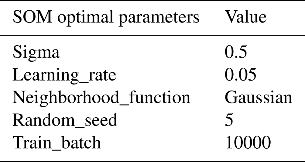
The SOM nodes are the clustered large-scale circulation patterns, which need to be determined before implementing the SOM model. A fewer number of nodes in the SOM array cannot capture specific circulation patterns while a greater number of nodes will produce redundant circulation patterns that are similar. Therefore, choosing the optimal SOM node is critical. In this study, we have tested several SOM arrays by quantization and topological errors, including 2×2, 2×3, 2×4, and 3×4 nodes, and we found that six distinctive circulation patterns with a 2×3 configuration can provide enough details for physical interpretation and satisfactorily describe the variations of the synoptic situations in the Huaihe River basin. In this study, the SOM analysis is performed mainly using the Python miniSOM library (Vettigli, 2021), and the corresponding optimal parameters are summarized in Table 1.
3.2 CNN-LSTM model
CNN has the advantage of extracting distinctive spatial features from images, and LSTM has the ability to deal with temporal series data (Shen, 2018; LeCun et al., 2015). Considering that the precipitation is influenced by the surrounding topography and the weather state of the current day and the previous days, we develop a spatiotemporal deep neural network model by combining CNN and LSTM. We build the model in the following steps:
-
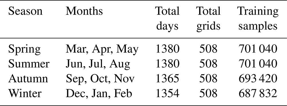
Data preparation. Taking summer precipitation as an example, first, each predictor is normalized to reduce the influence of different dimensions by min–max normalization. Second, we use the normalized data to construct input arrays with dimensions of , where 508 represents the number of precipitation grids in the basin, 1380 represents the number of summer days, 14 is the number of predictors (Table 2), and 3 represents the time dimension (i.e., t, t−1, and t−2). For each grid, a 5×5 sub-grid (about 125 km × 125 km) centered on it is extracted to fully consider the spatial information (Fig. S4). Third, in order to build models separately for each circulation pattern, we divide the input arrays into six groups based on the SOM results.
-
CNN model construction. Convolutional neural networks (CNNs) have been widely used in image recognition, object detection, and precipitation forecasting. It can extract more abstract features from the original image through a simple nonlinear model, avoiding the complex feature extraction process. As shown in Fig. 2, the CNN model includes an input layer with dimensions of , two convolutional layers, and a flattening layer. The convolution layer can extract informative local features from the input layer, and the flattening layer converts the matrix into a one-dimensional feature vector that is used as the input to the LSTM layer (Amini et al., 2022). Among them, the kernel size of the first convolutional layer is set to , where 32 is the output channel number, and 3×3 is the size of the kernel. To avoid overfitting and accelerate the training, batch normalization is applied to convolution layers (Pan et al., 2019).
-
LSTM model construction. The recurrent neural network (RNN) is a kind of neural network for processing sequence data, which can mine time series and semantic information from data. As a special RNN model, the long short-term memory network (LSTM) can overcome the vanishing and exploding gradient problems (Hochreiter and Schmidhuber, 1997). Besides this, the interactive operation among the input gate, output gate, and forget gate in LSTM enables the model to solve the long-term dependency problem (Huang and Kuo, 2018). As shown in Fig. 2, the LSTM model includes an input layer where the data come from the output of the CNN, a bidirectional LSTM layer with 16 hidden units, and a fully connected layer. Considering the impact of previous meteorological information on the precipitation, the input of the LSTM model not only includes the data of the current day but also 2 d ago (i.e., t−1 and t−2).
We select the Python package PyTorch as the framework of the above models and the NVIDIA A5000 GPU (graphics processing unit) to accelerate model training. The hyperparameters of models, such as learning rate, epochs, and batch size, are determined by the trial-and-error method. Furthermore, the above models are trained with the Adam optimization algorithm (Kingma and Ba, 2014).

3.3 Experimental design and statistical metrics
To answer the three questions in the introduction, we compare the SOM-CNN-LSTM method with three other benchmark methods including CNN, LSTM, and CNN-LSTM. The design differences of the four methods are shown in Table 3. Among them, the CNN-LSTM method is used to illustrate the effectiveness of circulation classification, while the CNN and LSTM methods are used to illustrate the importance of the incorporation of temporal and spatial information. Besides this, the precipitation forecast skill continuously decreases with increasing lead times, so we build the post-processing method for each lead time separately. This means that only for the SOM-CNN-LSTM method, we need to build models, where 15 represents the number of lead times, 6 represents the number of circulation patterns, and 4 represents different seasons. Therefore, to improve work efficiency, we first filter out the optimal parameter combination for one model and then adjust other model parameters based on that. In addition, each season has different training samples (Table 4), and we use four-fold cross-validation to calibrate and evaluate the model accuracy. For four-fold cross-validation, the 15 years of datasets are randomly grouped into four groups, and one group of datasets is selected as validation data, while the other groups of datasets are used as the training data to fit the statistical post-processing models (i.e., SOM-CNN-LSTM, CNN, LSTM, and CNN-LSTM). This step will be repeated four times until all datasets are used for validation.
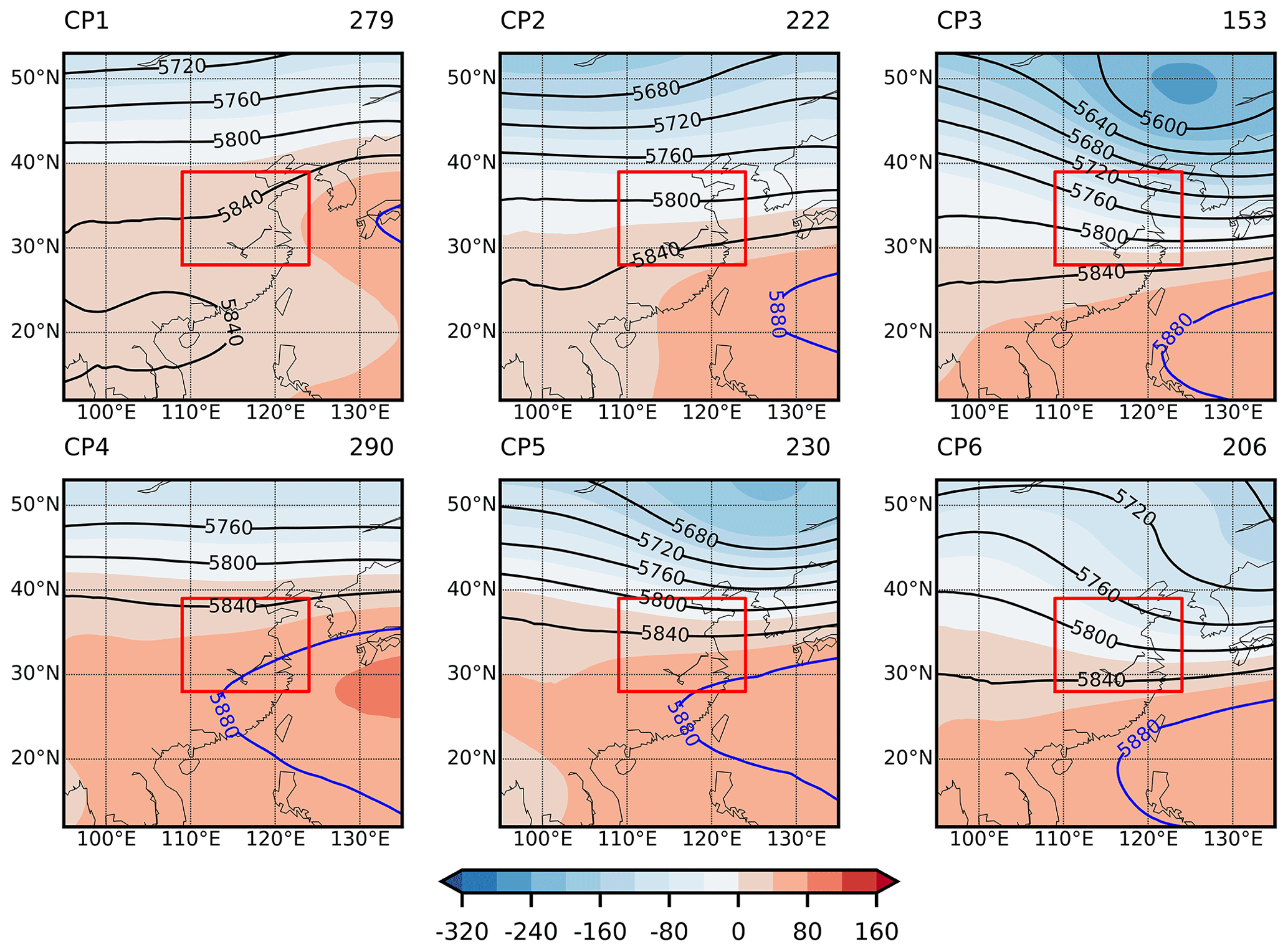
Figure 3Circulation patterns at the lead time of 1 d in the summer of 2007–2021. The blue bold line (5880 gpm) is the characteristic position of the WPSH, the red rectangle represents the scope of the Huaihe River basin, the colored shading stands for the geopotential height anomalies at 500 hPa, and the numbers for each circulation pattern are shown in the upper right corner.

To evaluate the performance of the post-processing results, three statistical metrics are selected, including root mean square error (RMSE), correlation coefficient (CC), and relative bias (RB).
where Pi and Oi represent simulated and observed precipitation at the ith point, respectively; and denote the average simulated and observed precipitation, respectively; and n is the number of samples.
4.1 Linkages between large-scale circulation patterns and precipitation
Figure 3 presents six large-scale circulation patterns at the lead time of 1 d in the summer of 2007–2021. It can be seen that the SOM model can well capture the key atmospheric circulation of the western Pacific subtropical high (WPSH) that affects the summer precipitation in eastern China (Zhou et al., 2020). For the WPSH, pattern CP1 exceeds 30∘ N in the eastern zone of the Huaihe River basin, pattern CP4 extends westward to 113∘ E and reaches the southeast zone of the basin, while pattern CP3 is in the southeast zone of the basin and is located around 20∘ N. From the perspective of geopotential height anomalies, patterns CP2, CP3, CP5, and CP6 have similar features, with negative (positive) 500 hPa geopotential height anomalies to the north (south) of the basin, while CP1 and CP4 have positive anomalies in the entire basin.
Table 5Contribution of different circulation patterns (CPs) to summer precipitation at a lead time of 1 d during 2007–2021.
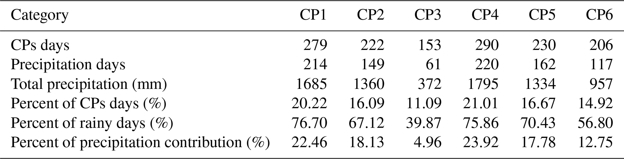
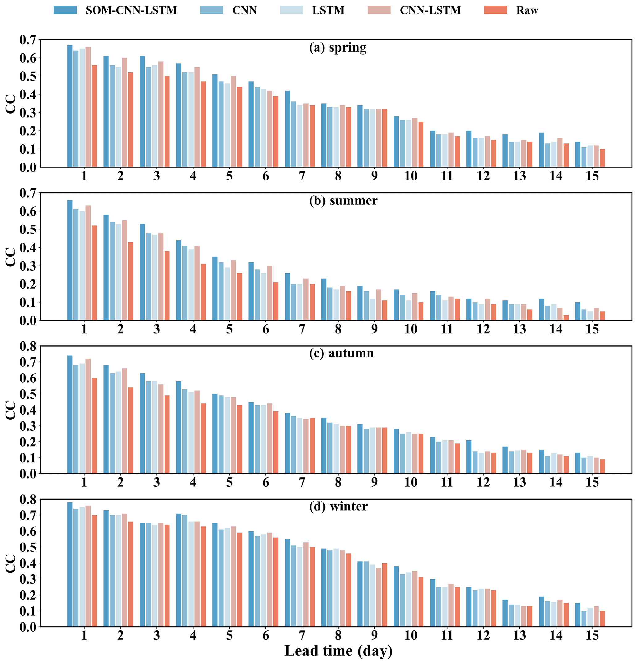
Figure 4Correlation coefficient (CC) of different methods over 1–15 lead days in four seasons.
To further characterize the relationship between circulation patterns and precipitation, we calculate the percent of each circulation pattern, the percent of rainy days, and the percent of precipitation contribution, which can be seen in Table 5. In general, CP1 and CP4 are frequent circulation patterns, and they contribute most to total summer precipitation, exceeding 40 %. In contrast, CP3 has the lowest frequency (11.09 %) with a small contribution to precipitation (only 4.96 %). Besides this, precipitation is more likely to occur in CP1 (76.70 %) and CP4 (75.86 %), although it can occur in any circulation pattern. The above results show that the change of WPSH (moving westward and expanding northward) exerts considerable impacts on precipitation in the Huaihe River basin. On the other hand, it also indirectly confirms the effectiveness of the circulation classification.
Considering that precipitation mainly occurs in summer, we only take this season as an example to analyze the results of large-scale circulation patterns and its statistical relationship with precipitation. The results of other seasons are shown in Supplement.
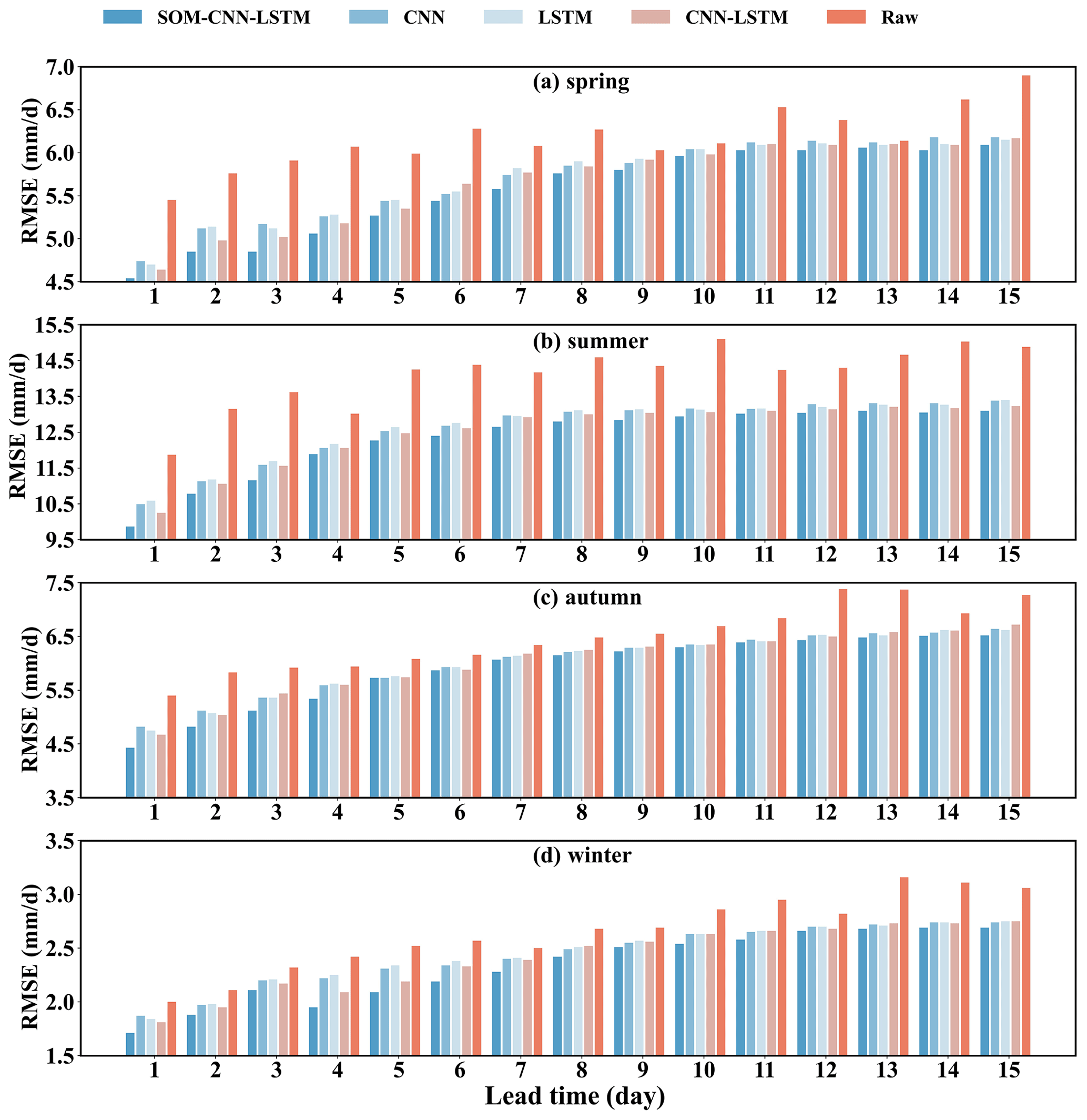
Figure 5Root mean square error (RMSE) of different methods over 1–15 lead days in four seasons.
4.2 Overall performance of different post-processing methods
Figure 4 shows the values of CC for different post-processing methods (i.e., SOM-CNN-LSTM, CNN, LSTM, CNN-LSTM) over 1–15 lead days during spring, summer, autumn, and winter. Overall, for each lead day and season, the four methods generally perform better than the raw forecasts. For example, the CC of the four methods ranges from 0.05 to 0.78, increased by an average of 18.69 % compared with the raw forecasts. Particularly, the SOM-CNN-LSTM method performs best, followed by CNN-LSTM, CNN, and LSTM. For instance, compared with the raw forecasts, the CC values of the SOM-CNN-LSTM method increase by an average of 32.30 %, followed by 16.90 % (CNN-LSTM), 13.42 % (CNN), and 12.15 % (LSTM).
As shown in Fig. 5, the raw forecasts have a relatively higher RMSE, and once the four post-processing methods are applied, RMSE values of the four seasons are largely decreased. Once again, the SOM-CNN-LSTM method exhibits preferable performance with the lowest RMSE. For example, compared with the raw forecasts, the RMSE of the SOM-CNN-LSTM method decreases by an average of 26.58 %, followed by 23.64 % (CNN-LSTM), 22.16 % (CNN), and 21.86 % (LSTM).
The relative bias (RB) of the four post-processing methods is shown in Fig. 6. Similar to the above results, the SOM-CNN-LSTM method has the lowest RB. Taking summer precipitation as an example, the average RB of the SOM-CNN-LSTM method is 1.83 %, CNN-LSTM is 2.12 %, CNN is 2.35 %, and the LSTM is 2.40 %, while the average RB of the raw forecasts is highest, reaching 2.6 %, which further illustrates that the SOM-CNN-LSTM method outperforms other methods. Besides this, forecast precipitation is overestimated in spring, summer, and winter, and it is underestimated in autumn. For example, for the optimal SOM-CNN-LSTM method, precipitation is overestimated by 11.12 % in spring, 1.83 % in summer, 11.42 % in winter, and underestimated by 4.17 % in autumn. Particularly, the underestimation of the SOM-CNN-LSTM method is especially visible during the fourth lead time of summer and autumn, exceeding 15 %.
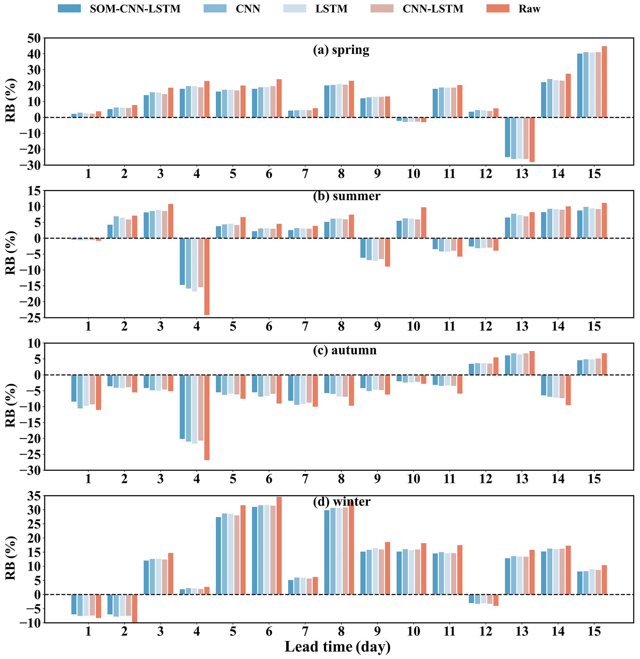
From the above results of three statistical metrics, the proposed SOM-CNN-LSTM post-processing method outperforms the no-circulation-pattern method (CNN-LSTM), the no-temporal information method (CNN), and the no-spatial information method (LSTM) at all lead times and each season, indicating that incorporating large-scale circulation patterns with local spatiotemporal information (e.g., elevation, specific humidity, and mean sea level pressure) can improve forecast skills.
We further adopt the CC, RMSE, and RB to compare the correction skills of the optimal SOM-CNN-LSTM method in different seasons and lead times. As shown in Fig. 7a and c, the values of CC (RMSE) continuously decrease (increase) with increasing lead times, which indicates the precipitation forecast skill has deteriorated over time. Taking 0.4 as the limit of CC, the effective lead time is 9 d in winter, 7 d in spring and autumn, and only 3 d in summer. In addition, winter forecast precipitation has the highest CC and lowest RMSE, followed by spring, autumn, and summer. However, winter precipitation has a larger RB compared with other seasons (Fig. 7e); the reason is that a small deviation may lead to a large relative bias. The above results indicate that winter forecast precipitation performs better than other seasons, especially in summer, which is consistent with previous studies (Buizza et al., 1999). As shown in Fig. 7b and d, the improvement of CC (RMSE) is highest in summer with an average of 0.09 (1.78), followed by 0.07 (0.60) in autumn, 0.06 (0.60) in spring, and 0.05 (0.32) in winter, indicating that the SOM-CNN-LSTM method has better correction skills in summer. The further comparison reveals that, while the precipitation forecast performance in winter is superior, the corrective ability is weaker. Although the summer precipitation forecast performance is not as good as the winter, it displays superior correction skills.
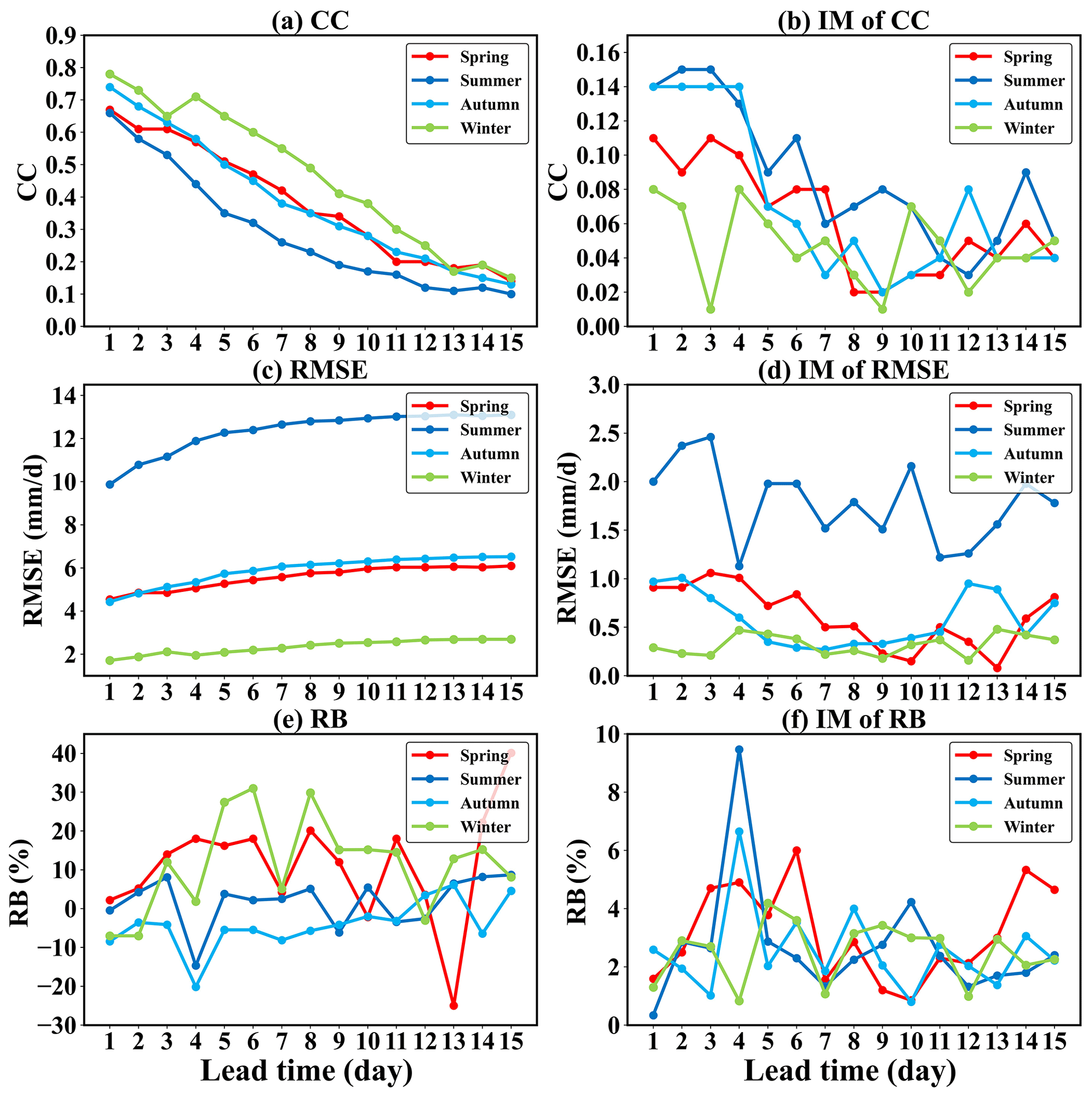
Figure 7(a) CC, (c) RMSE, and (e) RB of SOM-CNN-LSTM method over 1–15 lead days during spring, summer, autumn, and winter. The second column is the (b) improvement (IM) of CC, (d) RMSE, and (f) RB relative to raw forecasts.
Since the above results show that the SOM-CNN-LSTM method has the best performance, we only use it to analyze the spatial correction skills. The first two columns in Fig. 8 show the spatial distribution of CC for the SOM-CNN-LSTM method and raw forecasts at the lead time of 1 d, revealing the significant seasonal differences in CC. For instance, for most regions of the Huaihe River basin, winter raw forecasts have the highest CC (0.55–0.75), followed by autumn (0.45–0.71), spring (0.42–0.68), and summer (0.40–0.60), and this trend remains unchanged after SOM-CNN-LSTM correction. The third column indicates that the CC values exhibit improvement in all seasons for most regions of the basin after bias correction. Particularly, most regions in summer and the midlands in autumn show the better correction skill (Fig. 8f and i), whereas south and northwest of the basin in spring generally show a poorer performance (Fig. 8c), and winter has the lowest improvement of CC. In addition, all seasons have relatively poor correction skills in the northwest, which may be related to the higher topography in the region. The spatial distribution of the RMSE is similar to Fig. 8, which is shown in the Supplement (Fig. S5).
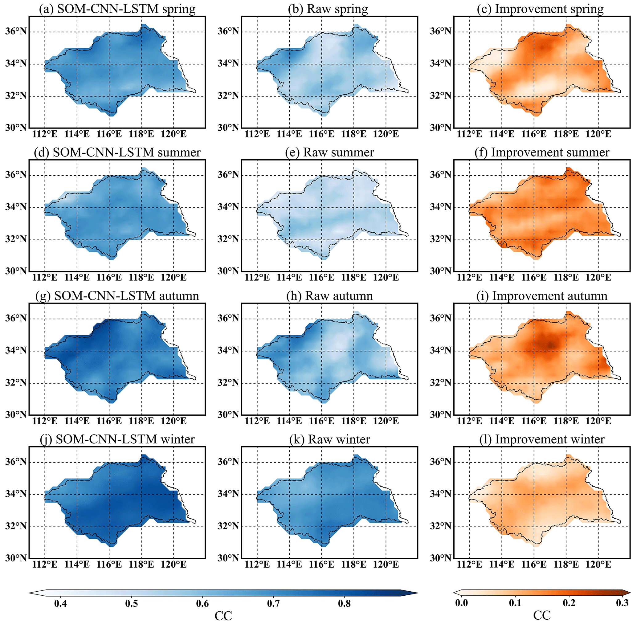
Figure 8Spatial distributions of the CC for the SOM-CNN-LSTM method and raw forecasts at a lead time of 1 d. The third column is the improvement of CC in spring, summer, autumn and winter.
4.3 Evaluation of interannual and different precipitation intensities in summer
4.3.1 Interannual assessment of different methods
In the previous section, we mainly focus on analyzing the overall and spatial forecast skills of different post-processing methods. The forecast skills of precipitation in the time dimension may be also different. Therefore, in this subsection, we take the summer precipitation as an example to analyze the annual forecast skills of different methods. Figure 9 presents the RB of four methods for each summer over 1–15 lead days during 2007–2021. Overall, for each year and most lead times, the SOM-CNN-LSTM method performs best with the lowest RB, lowest RMSE (Fig. S7), and highest CC (Fig. S8). In addition, there are significant interannual differences in the forecast performance. For example, precipitation of all four methods is significantly underestimated for most lead times in 2018, 2019, and 2021, and it is overestimated in 2009, 2011, and 2012. Furthermore, when the lead time exceeds 12 d, forecast precipitation is overestimated in most years, especially in 2013 and 2014. This significant interannual difference may be related to large-scale circulation configuration. Besides this, forecast precipitation has larger biases in 2007, 2020, and 2021 compared with other years (Fig. S7), and the CC is below 0.4 in most years when the lead time exceeds 3 d (Fig. S8).

Figure 9RB of different methods for each summer over 1–15 lead days from 2007 to 2021. The asterisk (*) indicates the best method with the lowest RB for each lead time.
4.3.2 Performance under different precipitation intensities
We further investigate the performance of four post-processing methods at different intensities, namely 0–1, 1–5, 5–10, 20–40, and ≥40 mm d−1, corresponding to no rain, light rain, moderate rain, heavy rain, and violent rain, respectively (Zambrano-Bigiarini et al., 2017). Considering that precipitation mainly occurs in summer, we take the season as an example for analysis. As shown in Fig. 10, the values of RMSE for all post-processing methods are lower than raw forecasts at different precipitation intensities, especially for no rain, light rain, and moderate rain events, which indicates that the four post-processing methods can reduce the bias and significantly improve the forecast skills. Clearly, the SOM-CNN-LSTM method achieves better scores than other methods in terms of the lowest RMSE. For example, compared with the raw forecasts, the RMSE values of the SOM-CNN-LSTM method in moderate rain events (Fig. 10c) decrease by an average of 39.70 %, followed by 36.02 % (CNN-LSTM), 34.95 % (CNN), and 33.91 % (LSTM). For heavy and violent rain events, the SOM-CNN-LSTM method has relatively better performance under lead times ranging from 1 to 7 d, with the RMSE decreasing by 14.85 % and 3.05 %, respectively, whereas the advantage is no longer obvious when the lead time exceeds 7 d; the values of RMSE only decrease by 5.4 % and 2.34 %, respectively. We can also get the similar conclusion from the CC and RB (Figs. S9 and S10). The reason is that the accuracy of forecast skills decreases with increasing lead times, and on the other hand, few violent rain events cannot provide enough training samples for deep learning models. In addition, there is a large RB between for both no rain and light rain (Fig. S9), which may be due to a small deviation leading to a large relative bias.
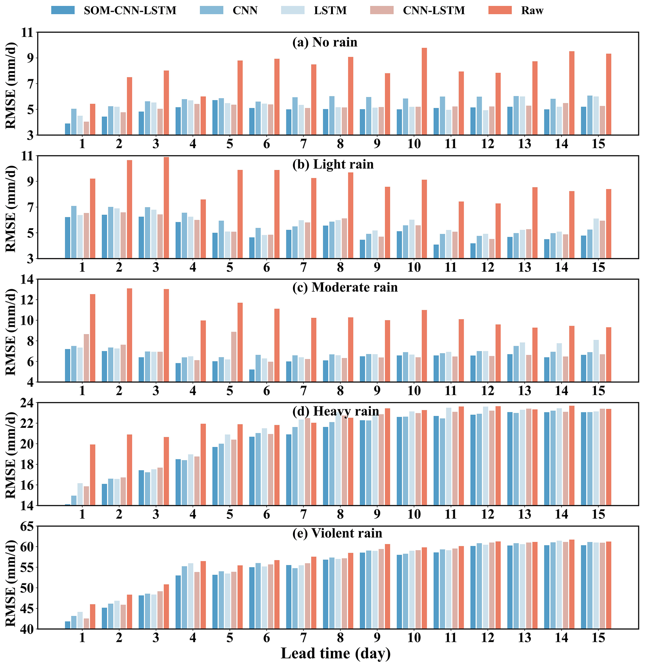
Figure 10RMSE of different methods over 1–15 lead days in summer at different intensities of (a) no rain, (b) light rain, (c) moderate rain, (d) heavy rain, and (e) violent rain.
Raw precipitation forecasts usually exhibit systematic and random errors due to the initial condition, boundary condition errors, and model structural errors from NWP. Prior work has documented the effectiveness of statistical post-processing techniques in reducing these biases and improving the accuracy of NWP. For instance, Scheuerer and Hamill (2015) presented a parametric post-processing method by fitting censored, shifted gamma distributions to access the conditional distribution of observed precipitation, which can significantly improve forecast skills. Particularly, for the Huaihe River basin, Tao et al. (2014) adopted the ensemble pre-processor (EPP) method to calibrate the TIGGE multi-model ensemble forecast precipitation, and Li et al. (2022b) adopted the CNN model to correct raw forecast precipitation by considering multi-spatial information. Although the above results show that post-processed precipitation forecasts have substantial improvement over the raw forecasts, these traditional post-processing methods overlook the influence of large-scale circulations and spatiotemporal information on precipitation. To overcome the problem, we propose the SOM-CNN-LSTM post-processing method. We compare the method with other benchmarks, including CNN, LSTM, and CNN-LSTM methods. The findings of this research are as follows.
Firstly, the SOM model can well capture the westward and northward movement of the WPSH, the primary circulation system influencing summer precipitation in eastern China, suggesting the effectiveness of circulation classification using SOM. The SOM-CNN-LSTM method performs better than the CNN-LSTM method in terms of three statistical metrics, indicating the effectiveness of considering the large-scale circulation patterns to correct the forecast precipitation. Secondly, the SOM-CNN-LSTM method performs better than CNN and LSTM methods, which indicates that considering both temporal and spatial information can improve forecast skills.
There are a growing number of deep learning models for statistical post-processing of numerical weather prediction, such as CNN (Pan et al., 2019) and ConvLSTM (Shi et al., 2015). The highlight of our work is the effective combination of the advantages of CNN for spatial data and LSTM for time series. On the other hand, through circulation classification, the effective information of the large-scale circulation pattern (i.e., westward and northward movement of the WPSH) is subtly integrated into the deep learning model.
However, some limitations still need to be further studied. Firstly, we primarily use 500 hPa geopotential height for circulation classification: more circulation variables such as column-integrated moisture fluxes (Zhang et al., 2022), sea level pressure (Loikith et al., 2017), and vertical velocity (Schlef et al., 2019) can also be used to represent the large-scale circulation patterns. Particularly, persistence and/or transitioning of circulation patterns may influence the local precipitation, which can be incorporated into the post-processing frame (Roller et al., 2016). Secondly, the SOM-CNN-LSTM method has relatively poor performance in heavy and violent rain when the lead time exceeds 7 d, which can be attributed to the limited violent rain samples training the model. Therefore, more studies on how to improve the forecast skills of violent rain should be carried out (Chen and Wang, 2022; Li et al., 2018). Thirdly, the spatiotemporal deep neural network can significantly improve the precipitation forecast skills; however, as a black box model, interpretability and understanding have been seen as potential weaknesses (Guidotti et al., 2019; Reichstein et al., 2019), meaning that we cannot understand how these predictors (e.g., elevation, specific humidity, and mean sea level pressure) affect the precipitation process. It will be valuable to consider interpretability in post-processing.
In this study, we propose the SOM-CNN-LSTM statistical post-processing method that combines large-scale circulation patterns with local spatiotemporal information to correct the raw ECMWF forecast precipitation over 1–15 lead days in the Huaihe River basin from 2007 to 2021. The proposed method is systematically evaluated with other benchmark methods (i.e., CNN, LSTM, and CNN-LSTM) in terms of root mean square error, correlation coefficient, and relative bias, and it is also evaluated from space-scale, timescale, and intensity. The main conclusions of the study are as follows:
-
The SOM model can effectively classify the large-scale circulation patterns over the Huaihe River basin. Particularly, the SOM can well capture the westward and northward movement of the western pacific subtropical high, and the corresponding circulation patterns CP1 and CP4 contribute the most to the total summer precipitation, exceeding 40 %.
-
The proposed SOM-CNN-LSTM post-processing method outperforms the no-circulation-pattern method (CNN-LSTM), the no-temporal information method (CNN), and the no-spatial information method (LSTM) at all lead times and each season, and the optimal method has the largest correlation coefficient improvement (32.30 %) and root mean square error reduction (26.58 %). The results indicate incorporating large-scale circulation patterns with local spatiotemporal information can improve forecasting skills.
-
There are significant seasonal and interannual differences in the forecast skills of precipitation. Winter precipitation has better forecast skills than summer, whereas summer precipitation has better correction skills than winter. Summer precipitation is significantly underestimated in 2018, 2019, and 2021, and it is overestimated in 2009, 2011, and 2012. Furthermore, when the lead time exceeds 12 d, forecast precipitation is overestimated in most years, especially in 2013 and 2014.
-
The SOM-CNN-LSTM method also performs best for different precipitation intensities. Particularly, for heavy and violent rain events, the SOM-CNN-LSTM method has relatively better performance under lead times ranging from 1 to 7 d, whereas the advantage is no longer obvious when the lead time exceeds 7 d, which can be attributed to the limited precipitation samples for training the model.
In summary, this study provides a feasible and effective post-processing method to improve precipitation forecasting skills, which would benefit hydrological forecasts and other applications.
The CN05.1 daily precipitation dataset can be obtained from Wu and Gao (2013). Forecast precipitation, meteorological factors, and 500 hPa geopotential height are from the forecast dataset of ECMWF and can be obtained from the following website: https://apps.ecmwf.int/datasets/data/tigge (ECMWF, 2023). Topography can be obtained from the Geospatial Data Cloud of China (http://www.gscloud.cn/#page1/1, GDCC, 2023). The code used in this study is available from the authors upon request.
The supplement related to this article is available online at: https://doi.org/10.5194/hess-27-1945-2023-supplement.
ZL: conceptualization, methodology, and funding acquisition; TZ: data preparation, software, validation, visualization, and writing – original draft; WL: supervision and data analysis; JW: supervision; YH: reviewing; and BL: reviewing.
The contact author has declared that none of the authors has any competing interests.
Publisher's note: Copernicus Publications remains neutral with regard to jurisdictional claims in published maps and institutional affiliations.
The authors are grateful to Chenglin Bi (Hohai University, China) and Lingjie Li (Nanjing Hydraulic Research Institute, China) for their participation in the analysis of the large-scale circulation patterns. The authors also thank the anonymous reviewers for their constructive comments and Xing Yuan for handling the manuscript.
This study is supported by the Postgraduate Research & Practice Innovation Program of Jiangsu Province, the Fundamental Research Funds for the Central Universities of China, and the National Natural Science Foundation of China (grant nos. 41730750 and 41877147).
This paper was edited by Xing Yuan and reviewed by three anonymous referees.
Amini, A., Dolatshahi, M., and Kerachian, R.: Adaptive precipitation nowcasting using deep learning and ensemble modeling, J. Hydrol., 612, 128197, https://doi.org/10.1016/j.jhydrol.2022.128197, 2022.
Bauer, P., Thorpe, A., and Brunet, G.: The quiet revolution of numerical weather prediction, Nature, 525, 47–55, https://doi.org/10.1038/nature14956, 2015.
Bougeault, P., Toth, Z., Bishop, C., Brown, B., Burridge, D., Chen, D. H., Ebert, B., Fuentes, M., Hamill, T. M., Mylne, K., Nicolau, J., Paccagnella, T., Park, Y.-Y., Parsons, D., Raoult, B., Schuster, D., Dias, P. S., Swinbank, R., Takeuchi, Y., Tennant, W., Wilson, L., and Worley, S.: The THORPEX interactive grand global ensemble, B. Am. Meteorol. Soc., 91, 1059–1072, https://doi.org/10.1175/2010bams2853.1, 2010.
Bremnes, J. B.: Probabilistic forecasts of precipitation in terms of quantiles using NWP model output, Mon. Weather Rev., 132, 338–347, https://doi.org/10.1175/1520-0493(2004)132<0338:PFOPIT>2.0.CO;2, 2004.
Buizza, R., Milleer, M., and Palmer, T. N.: Stochastic representation of model uncertainties in the ECMWF ensemble prediction system, Q. J. Roy. Meteorol. Soc., 125, 2887–2908, https://doi.org/10.1002/qj.49712556006, 1999.
Chen, C., Jiang, J., Liao, Z., Zhou, Y., Wang, H., and Pei, Q.: A short-term flood prediction based on spatial deep learning network: A case study for Xi County, China, J. Hydrol., 607, 127535, https://doi.org/10.1016/j.jhydrol.2022.127535, 2022.
Chen, G. and Wang, W. C.: Short-Term Precipitation Prediction for Contiguous United States Using Deep Learning, Geophys. Res. Lett., 49, e2022GL097904, https://doi.org/10.1029/2022gl097904, 2022.
Clark, M., Gangopadhyay, S., Hay, L., Rajagopalan, B., and Wilby, R.: The Schaake shuffle: A method for reconstructing space–time variability in forecasted precipitation and temperature fields, J. Hydrometeorol., 5, 243–262, https://doi.org/10.1175/1525-7541(2004)005<0243:TSSAMF>2.0.CO;2, 2004.
ECMWF – European Centre for Medium-Range Weather Forecasts: TIGGE Data Retrieval, https://apps.ecmwf.int/datasets/data/tigge (last access: 11 May 2023), 2023.
Ford, T. W., Quiring, S. M., Frauenfeld, O. W., and Rapp, A. D.: Synoptic conditions related to soil moisture-atmosphere interactions and unorganized convection in Oklahoma, J. Geophys. Res.-Atmos., 120, 11519–11535, https://doi.org/10.1002/2015jd023975, 2015.
GDCC – Geospatial Data Cloud of China: Remote Sensing Data Retrieval, http://www.gscloud.cn/#page1/1 (last access: 11 May 2023), 2023.
Ghazvinian, M., Zhang, Y., Seo, D. J., He, M., and Fernando, N.: A novel hybrid artificial neural network – Parametric scheme for postprocessing medium-range precipitation forecasts, Adv. Water Resour., 151, 103907, https://doi.org/10.1016/j.advwatres.2021.103907, 2021.
Gneiting, T. and Raftery, A. E.: Weather forecasting with ensemble methods, Science, 310, 248–249, https://doi.org/10.1126/science.1115255, 2005.
Guidotti, R., Monreale, A., Ruggieri, S., Turini, F., Giannotti, F., and Pedreschi, D.: A survey of methods for explaining black box models, ACM Comput. Surv., 51, 1–42, https://doi.org/10.1145/3236009, 2019.
Hamill, T. M.: Verification of TIGGE multimodel and ECMWF reforecast-calibrated probabilistic precipitation forecasts over the contiguous United States, Mon. Weather Rev., 140, 2232–2252, https://doi.org/10.1175/mwr-d-11-00220.1, 2012.
Herman, G. R. and Schumacher, R. S.: Money doesn't grow on trees, but forecasts do: Forecasting extreme precipitation with random forests, Mon. Weather Rev., 146, 1571–1600, https://doi.org/10.1175/mwr-d-17-0250.1, 2018.
Hochreiter, S. and Schmidhuber, J.: Long short-term memory, Neural Comput., 9, 1735–1780, https://doi.org/10.1162/neco.1997.9.8.1735, 1997.
Horton, D. E., Johnson, N. C., Singh, D., Swain, D. L., Rajaratnam, B., and Diffenbaugh, N. S.: Contribution of changes in atmospheric circulation patterns to extreme temperature trends, Nature, 522, 465–469, https://doi.org/10.1038/nature14550, 2015.
Huang, C. J. and Kuo, P. H.: A Deep CNN-LSTM Model for Particulate Matter (PM2.5) Forecasting in Smart Cities, Sensors, 18, 2220, https://doi.org/10.3390/s18072220, 2018.
Huang, L. and Luo, Y.: Evaluation of quantitative precipitation forecasts by TIGGE ensembles for south China during the presummer rainy season, J. Geophys. Res.-Atmos., 122, 8494–8516, https://doi.org/10.1002/2017jd026512, 2017.
Kingma, D. P. and Ba, J.: Adam: A method for stochastic optimization, arXiv [preprint], arXiv:1412.6980, https://doi.org/10.48550/arXiv.1412.6980, 2014.
Kohonen, T.: The self-organizing map, Proc. IEEE, 78, 1464–1480, https://doi.org/10.1109/5.58325, 1990.
LeCun, Y., Bengio, Y., and Hinton, G.: Deep learning, Nature, 521, 436–444, https://doi.org/10.1038/nature14539, 2015.
Li, J., Sharma, A., Evans, J., and Johnson, F.: Addressing the mischaracterization of extreme rainfall in regional climate model simulations – A synoptic pattern based bias correction approach, J. Hydrol., 556, 901–912, https://doi.org/10.1016/j.jhydrol.2016.04.070, 2018.
Li, M., Jiang, Z., Zhou, P., Le Treut, H., and Li, L.: Projection and possible causes of summer precipitation in eastern China using self-organizing map, Clim. Dynam., 54, 2815–2830, https://doi.org/10.1007/s00382-020-05150-4, 2020.
Li, Q., Wang, Z., Shangguan, W., Li, L., Yao, Y., and Yu, F.: Improved daily SMAP satellite soil moisture prediction over China using deep learning model with transfer learning, J. Hydrol., 600, 126698, https://doi.org/10.1016/j.jhydrol.2021.126698, 2021.
Li, W., Duan, Q., Wang, Q. J., Huang, S., and Liu, S.: Evaluation and statistical post-processing of two precipitation reforecast products during summer in the mainland of China, J. Geophys. Res.-Atmos., 127, e2022JD036606, https://doi.org/10.1029/2022jd036606, 2022a.
Li, W., Pan, B., Xia, J., and Duan, Q.: Convolutional neural network-based statistical post-processing of ensemble precipitation forecasts, J. Hydrol., 605, 127301, https://doi.org/10.1016/j.jhydrol.2021.127301, 2022b.
Liu, W., Wang, L., Chen, D., Tu, K., Ruan, C., and Hu, Z.: Large-scale circulation classification and its links to observed precipitation in the eastern and central Tibetan Plateau, Clim. Dynam., 46, 3481–3497, https://doi.org/10.1007/s00382-015-2782-z, 2016.
Liu, Y., Duan, Q., Zhao, L., Ye, A., Tao, Y., Miao, C., Mu, X., and Schaake, J. C.: Evaluating the predictive skill of post-processed NCEP GFS ensemble precipitation forecasts in China's Huai river basin, Hydrol. Process., 27, 57–74, https://doi.org/10.1002/hyp.9496, 2013.
Loikith, P. C., Lintner, B. R., and Sweeney, A.: Characterizing large-scale meteorological patterns and associated temperature and precipitation extremes over the northwestern United States using self-organizing maps, J. Climate, 30, 2829–2847, https://doi.org/10.1175/jcli-d-16-0670.1, 2017.
Mechem, D. B., Wittman, C. S., Miller, M. A., Yuter, S. E., and de Szoeke, S. P.: Joint synoptic and cloud variability over the Northeast Atlantic near the Azores, J. Appl. Meteorol. Clim., 57, 1273—1290, https://doi.org/10.1175/jamc-d-17-0211.1, 2018.
Ning, L., Liu, J., and Wang, B.: How does the South Asian high influence extreme precipitation over eastern China?, J. Geophys. Res.-Atmos., 122, 4281–4298, https://doi.org/10.1002/2016jd026075, 2017.
Pan, B., Hsu, K., AghaKouchak, A., and Sorooshian, S.: Improving precipitation estimation using convolutional neural network, Water Resour. Res., 55, 2301–2321, https://doi.org/10.1029/2018wr024090, 2019.
Peng, T., Zhi, X., Ji, Y., Ji, L., and Tian, Y.: Prediction skill of extended range 2-m maximum air temperature probabilistic forecasts using machine learning post-processing methods, Atmosphere, 11, 823, https://doi.org/10.3390/atmos11080823, 2020.
Raftery, A. E., Gneiting, T., Balabdaoui, F., and Polakowski, M.: Using Bayesian model averaging to calibrate forecast ensembles, Mon. Weather Rev., 133, 1155–1174, https://doi.org/10.1175/MWR2906.1, 2005.
Reichstein, M., Camps-Valls, G., Stevens, B., Jung, M., Denzler, J., Carvalhais, N., and Prabhat, P.: Deep learning and process understanding for data-driven Earth system science, Nature, 566, 195–204, https://doi.org/10.1038/s41586-019-0912-1, 2019.
Roller, C. D., Qian, J.-H., Agel, L., Barlow, M., and Moron, V.: Winter weather regimes in the Northeast United States, J. Climate, 29, 2963–2980, https://doi.org/10.1175/JCLI-D-15-0274.1, 2016.
Schefzik, R., Thorarinsdottir, T. L., and Gneiting, T.: Uncertainty quantification in complex simulation models using ensemble copula coupling, Stat. Sci., 28, 616–640, https://doi.org/10.1214/13-sts443, 2013.
Scheuerer, M. and Hamill, T. M.: Statistical postprocessing of ensemble precipitation forecasts by fitting censored, shifted gamma distributions, Mon. Weather Rev., 143, 4578–4596, https://doi.org/10.1175/mwr-d-15-0061.1, 2015.
Schlef, K. E., Moradkhani, H., and Lall, U.: Atmospheric circulation patterns associated with extreme United States floods identified via machine learning, Sci. Rep., 9, 7171, https://doi.org/10.1038/s41598-019-43496-w, 2019.
Shen, C.: A transdisciplinary review of deep learning research and its relevance for water resources scientists, Water Resour. Res., 54, 8558–8593, https://doi.org/10.1029/2018wr022643, 2018.
Shi, X., Chen, Z., Wang, H., Yeung, D. Y., Wong, W. K., and Woo, W. C.: Convolutional LSTM network: A machine learning approach for precipitation nowcasting, Adv. Neural Info. Proc. Syst., 28, 802–810, 2015.
Shrestha, D. L., Robertson, D. E., Bennett, J. C., and Wang, Q. J.: Improving precipitation forecasts by generating ensembles through postprocessing, Mon. Weather Rev., 143, 3642–3663, https://doi.org/10.1175/MWR-D-14-00329.1, 2015.
Tao, Y., Duan, Q., Ye, A., Gong, W., Di, Z., Xiao, M., and Hsu, K.: An evaluation of post-processed TIGGE multimodel ensemble precipitation forecast in the Huai river basin, J. Hydrol., 519, 2890–2905, https://doi.org/10.1016/j.jhydrol.2014.04.040, 2014.
Vannitsem, S., Bremnes, J. B., Demaeyer, J., Evans, G. R., Flowerdew, J., Hemri, S., Lerch, S., Roberts, N., Theis, S., Atencia, A., Ben Bouallègue, Z., Bhend, J., Dabernig, M., De Cruz, L., Hieta, L., Mestre, O., Moret, L., Plenković, I. O., Schmeits, M., Taillardat, M., Van den Bergh, J., Van Schaeybroeck, B., Whan, K., and Ylhaisi, J.: Statistical postprocessing for weather forecasts: Review, challenges, and avenues in a big data world, B. Am. Meteorol. Soc., 102, E681–E699, https://doi.org/10.1175/bams-d-19-0308.1, 2021.
Veldkamp, S., Whan, K., Dirksen, S., and Schmeits, M.: Statistical postprocessing of wind speed forecasts using convolutional neural networks, Mon. Weather Rev., 149, 1141–1152, https://doi.org/10.1175/mwr-d-20-0219.1, 2021.
Vettigli, G.: Minisom, GitHub [code], https://github.com/JustGlowing/minisom (last access: 11 May 2023), 2021.
Wang, D., Jensen, M. P., Taylor, D., Kowalski, G., Hogan, M., Wittemann, B. M., Rakotoarivony, A., Giangrande, S. E., and Park, J. M.: Linking synoptic patterns to cloud properties and local circulations over southeastern Texas, Journal of Geophysical Research: Atmospheres, 127, e2021JD035920, https://doi.org/10.1029/2021jd035920, 2022.
Wang, J., Dong, X., Kennedy, A., Hagenhoff, B., and Xi, B.: A regime-based evaluation of southern and northern Great Plains warm-season precipitation events in WRF, Weather Forecast., 34, 805–831, https://doi.org/10.1175/waf-d-19-0025.1, 2019.
Wu, H., Yang, Q., Liu, J., and Wang, G.: A spatiotemporal deep fusion model for merging satellite and gauge precipitation in China, J. Hydrol., 584, 124664, https://doi.org/10.1016/j.jhydrol.2020.124664, 2020.
Wu, J. and Gao, X. J.: A gridded daily observation dataset over China region and comparison with the other datasets, Chinese J. Geophys., 56, 1102–1111, https://doi.org/10.6038/cjg20130406, 2013.
Xu, L., Chen, N., Yang, C., Yu, H., and Chen, Z.: Quantifying the uncertainty of precipitation forecasting using probabilistic deep learning, Hydrol. Earth Syst. Sci., 26, 2923–2938, https://doi.org/10.5194/hess-26-2923-2022, 2022.
Zambrano-Bigiarini, M., Nauditt, A., Birkel, C., Verbist, K., and Ribbe, L.: Temporal and spatial evaluation of satellite-based rainfall estimates across the complex topographical and climatic gradients of Chile, Hydrol. Earth Syst. Sci., 21, 1295–1320, https://doi.org/10.5194/hess-21-1295-2017, 2017.
Zhang, S., Chen, Y., Luo, Y., Liu, B., Ren, G., Zhou, T., Martinez-Villalobos, C., and Chang, M.: Revealing the circulation pattern most conducive to precipitation extremes in Henan Province of North China, Geophys. Res. Lett., 49, e2022GL098034, https://doi.org/10.1029/2022gl098034, 2022.
Zhang, X., Yang, H., Wang, X., Shen, L., Wang, D., and Li, H.: Analysis on characteristic and abnormality of atmospheric circulations of the July 2021 extreme precipitation in Henan, Trans. Atmos. Sci., 44, 672–687, 2021.
Zhang, Y. and Ye, A.: Machine learning for precipitation forecasts post-processing – Multi-model comparison and experimental investigation, J. Hydrometeorol., 22, 3065–3085, https://doi.org/10.1175/jhm-d-21-0096.1, 2021.
Zhou, B., Zhai, P., and Chen, Y.: Contribution of changes in synoptic-scale circulation patterns to the past summer precipitation regime shift in eastern China, Geophys. Res. Lett., 47, e2020GL087728, https://doi.org/10.1029/2020gl087728, 2020.