the Creative Commons Attribution 4.0 License.
the Creative Commons Attribution 4.0 License.
 | 15 May 2023
Hybrid forecasting: blending climate predictions with AI models
Louise J. Slater
Louise Arnal
Marie-Amélie Boucher
Annie Y.-Y. Chang
Simon Moulds
Conor Murphy
Grey Nearing
Guy Shalev
Chaopeng Shen
Linda Speight
Gabriele Villarini
Robert L. Wilby
Andrew Wood
Massimiliano Zappa
Hybrid hydroclimatic forecasting systems employ data-driven (statistical or machine learning) methods to harness and integrate a broad variety of predictions from dynamical, physics-based models – such as numerical weather prediction, climate, land, hydrology, and Earth system models – into a final prediction product. They are recognized as a promising way of enhancing the prediction skill of meteorological and hydroclimatic variables and events, including rainfall, temperature, streamflow, floods, droughts, tropical cyclones, or atmospheric rivers. Hybrid forecasting methods are now receiving growing attention due to advances in weather and climate prediction systems at subseasonal to decadal scales, a better appreciation of the strengths of AI, and expanding access to computational resources and methods. Such systems are attractive because they may avoid the need to run a computationally expensive offline land model, can minimize the effect of biases that exist within dynamical outputs, benefit from the strengths of machine learning, and can learn from large datasets, while combining different sources of predictability with varying time horizons. Here we review recent developments in hybrid hydroclimatic forecasting and outline key challenges and opportunities for further research. These include obtaining physically explainable results, assimilating human influences from novel data sources, integrating new ensemble techniques to improve predictive skill, creating seamless prediction schemes that merge short to long lead times, incorporating initial land surface and ocean/ice conditions, acknowledging spatial variability in landscape and atmospheric forcing, and increasing the operational uptake of hybrid prediction schemes.
- Article
(1554 KB) - Full-text XML
- BibTeX
- EndNote


This review addresses the growing popularity of hybrid forecasting, an approach that seeks to enhance the predictability of hydroclimatic variables by merging predictions from dynamical physics-based weather or climate simulation models with data-driven models. Dynamical models represent the temporal changes in system properties by using numerical modelling to solve dynamical physical processes. Data-driven models include empirical, statistical, and machine learning (ML) methods (i.e. can be described as artificial intelligence or AI) and can range from simple linear regression to deep neural networks. Recognizing that dynamical and AI models have different strengths, hybrid prediction reflects the deliberate fusing of the two.
(e.g. Vecchi et al., 2011; Slater and Villarini, 2018)(e.g. Schlef et al., 2021)(e.g. AghaKouchak et al., 2022)(e.g. Glahn and Lowry, 1972)Bennett et al. (2016)Richardson et al. (2020)(e.g. Watt-Meyer et al., 2021)(e.g. Madadgar et al., 2016)(e.g. Bogner et al., 2019)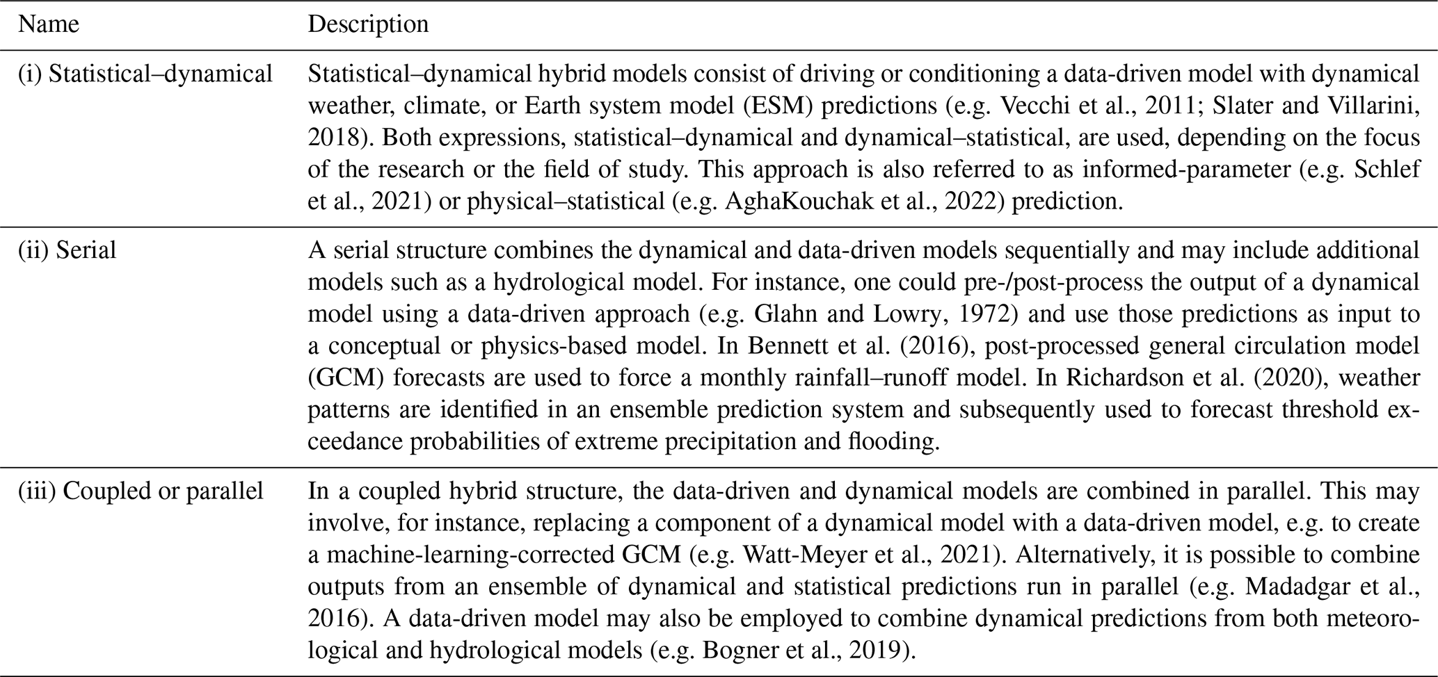
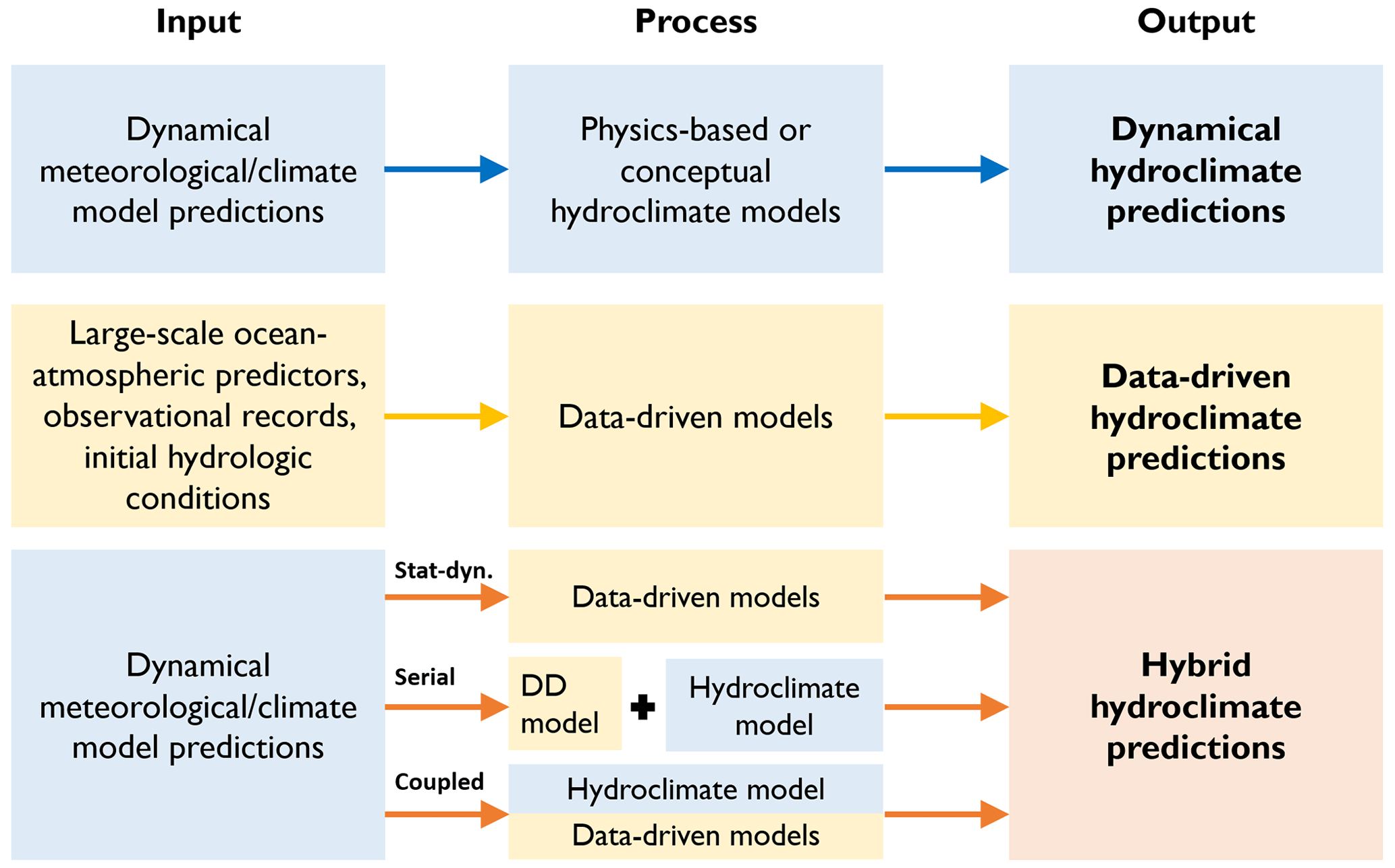
Figure 1Defining hybrid hydroclimate forecasting and prediction. The term “hydroclimate” refers to a range of variables defined in the text, including streamflow. The top row indicates the traditional dynamical hydroclimate predictions (blue), the middle row is data-driven (DD) predictions (yellow), and the bottom row represents hybrid predictions (red), which combine dynamical and data-driven approaches. In the last row, three examples of a hybrid structure are shown from top to bottom, namely (i) statistical–dynamical (Stat-dyn), (ii) serial, and (iii) coupled, as described in Table 1. The figure provides simple examples, but other schemes are possible, including, for example, a mix of observations and predictions in the left column.
Table 2Examples of hybrid forecasts of different hydroclimate variables and model types. Each example includes both a data-driven model and a dynamical weather or climate model. Examples are sorted by increasing time horizon. Hybrid model types are defined in Table 1, and the acronyms are defined in Table 3.
While challenging to identify distinct categories, given the flexibility and diversity of hybrid methods, three principal types of hybrid model structure may be discerned (Fig. 1; Table 1). These include (i) statistical–dynamical models that typically drive a statistical or ML model (data driven) with dynamical weather or climate model outputs from numerical weather prediction (NWP) models or Earth system models (ESMs). The statistical–dynamical structure is the most common type of hybrid model in the literature (Table 2). (ii) Serial models combine data-driven and dynamical models sequentially and may include additional types of models, such as a hydrological model. (iii) Coupled or parallel approaches combine data-driven and dynamical models in parallel. The coupled approach is more commonly employed in operational settings, where ML is increasingly being used to upgrade components within existing modelling schemes. We do not provide a prescriptive definition of hybrid forecasting, as it exists along a continuum from loosely to fully hybrid (e.g. AghaKouchak et al., 2022) and may include a wide range of models and big data, such as Earth observations (EOs).
Traditional workflows in which a physics-based or conceptual land/hydrology model generates the final forecast product are still the most commonly used operational forecasting systems worldwide. Physics-based models are based on a spatially distributed representation of known physical laws through mathematical equations and numerical solutions (e.g. Freeze and Harlan, 1969), while conceptual models simplify the representation of physical processes, often using empirical relationships (e.g. Nash and Sutcliffe, 1970). There is a long history of the development and application of standalone dynamical land surface and catchment hydrology models of varying complexity (from conceptual to physically explicit) for operational forecasting. Process-based hydrological modelling approaches may either be spatially distributed (gridded) or lumped (catchment averaged). Examples include the hourly conceptual rainfall–runoff GR4H (Génie Rural à 4 paramétres Horaires) model used by the Bureau of Meteorology in Australia (Hapuarachchi et al., 2022), the conceptual reservoir-based HSAMI model implemented by Hydro-Québec (Bisson and Roberge, 1983), or the conceptual Sacramento Soil Moisture Accounting (SAC-SMA) model of the Community Hydrologic Prediction System of the U.S. National Weather Service (Burnash et al., 1973). In operational systems, the hydrological model is typically forced with NWP-based forecast meteorology, as in the case of the U.S. National Water Model (NOAA, 2016; see Zappa et al., 2008, for a report on the science-driven operational application of several end-to-end ensemble hydrometeorological forecasting systems). Outputs from coupled atmosphere–ocean–land GCMs may be used over longer time horizons, as is the case with the European and Global Flood Awareness Systems, EFAS and GloFAS (Alfieri et al., 2013; Thielen et al., 2009; Smith et al., 2016; Arnal et al., 2018; Emerton et al., 2018; Harrigan et al., 2023). These approaches are considered to be more physically interpretable than black box statistical methods. However, the large computational demand and variable skill of many traditional forecasting approaches still persists (Arnal et al., 2018), and their calibration still requires substantial effort (Arheimer et al., 2020; Hirpa et al., 2018) relative to most data-driven models (see Sect. 3.4).
In contrast with traditional forecast workflows, data-driven prediction has historically relied more on observed data than dynamical climate model predictions, building empirical relationships between, for example, streamflow and precipitation (Garen, 1992), using time lag relationships between upstream and downstream flow, or stochastic autoregression approaches, like autoregressive moving average models (Jain et al., 2018). In such data-driven models, the hydroclimatological predictands can be regressed on a range of covariates, such as observed precipitation/temperature records, static variables (e.g. elevation, slope, and geology), initial hydrologic conditions, or large-scale predictors such as sea surface temperatures (SSTs), surface air temperature, geopotential height, meridional wind, sea ice extent, or modes of climate variability such as the El Niño–Southern Oscillation (ENSO; e.g. Wilby et al., 2004; Dixon and Wilby, 2019; Mendoza et al., 2017; Meißner et al., 2017). Broadly speaking, the strength of statistical models lies in their simplicity, speed, ease of use, and comparable skill to dynamical methods when there are sufficient observations for model training. However, data-driven models are sometimes thought to be less able to extrapolate to extreme outlier values that have not been seen in the historical record (Milly et al., 2008; Frame et al., 2022a; Reichstein et al., 2019) or unable to reflect shifts in the relationship between the predictand and predictors. Others have raised the risk of artificial skill in cases where predictors are selected preferentially based on the correlation with the predictand and are not fully cross-validated (e.g. DelSole and Shukla, 2009). Data-driven models may also be difficult to optimize for multi-variate, high-dimensional output fields, which are simulated intrinsically by dynamical models. Recent studies focusing on more complex data-driven techniques such as deep learning have suggested that some of these limitations can be overcome, such as the extrapolation to extreme or unforeseen conditions (Frame et al., 2022a), to new (untrained) catchments (Kratzert et al., 2019a), and to poorly gauged large regions (Feng et al., 2021; Ma et al., 2021). Nevertheless, the inclusion of physical constraints could further elevate the prediction robustness in data-sparse situations (Feng et al., 2022a). Research is required to understand the hydroclimatological conditions to which new ML and DL models are able to extrapolate from the training set and their performance as they are extrapolated in space.
Hybrid forecasts benefit from combining the ability of physical models to predict and explain large-scale phenomena (i.e. through NWPs or climate model predictions) with the ability of data-driven models to efficiently estimate the characteristics of events from observed data and account for bias or anomalies in the data. Many current examples of hybrid prediction build on traditional forecast workflows by using an ML algorithm in sequence with or alongside a conceptual or physics-based hydrological model (World Meteorological Organization, 2021; Fig. 1). Some notable examples of operational hybrid prediction include the objective consensus climate forecast (i.e. derived objectively from multiple models) at the U.S. Climate Prediction Center, which uses ensemble regression (e.g. Unger et al., 2009) to combine multiple dynamical and statistical forecasts into one. The International Research Institute for Climate and Society (IRI) has a multi-model-calibrated prediction based on three Subseasonal Experiment (SubX) models (Pegion et al., 2019). The UK Met Office uses a tool called Decider, which assigns medium-range precipitation forecast ensemble members to a set of 30 probabilistic weather patterns (Neal et al., 2016) and then feeds several downstream forecasting applications, such as for coastal flooding (Neal et al., 2018) and fluvial flooding (Richardson et al., 2020). Last, the Google flood forecasting model (https://sites.research.google/floods/, last access: 6 May 2023) produces operational, public-facing forecasts of water levels up to 6 d ahead (Nevo et al., 2022), using ML models forced with operational, real-time weather forecasts from the ECMWF Atmospheric Model high-resolution 10 d forecast (ECMWF HRES) as inputs. Broadly speaking, many hydroclimate projection systems are now hybrid, as per the serial definition in Table 1, because some kind of statistical processing is applied to generate a final information product from an ensemble of climate model outputs. Dynamical modelling centres often lack the resources or scope to tailor outputs to particular stakeholder needs (adding value with data-driven methods), leading to the implementation of such processing by the end-users themselves. These predictions are not always visible as hybrid activity but are operational nonetheless. These examples show the general evolution of the field from traditional forecasting (Cohen et al., 2019) toward hybrid prediction.
Table 3Modelling acronyms referred to in the paper. The top section includes data-driven models and approaches; the bottom section includes other acronyms used.


Figure 2Example of a seasonal hybrid forecasting system for maximum summer discharge at one stream gauge, using seasonal climate forecasts from eight climate models (94 members) of the NMME to drive a distributional regression model of streamflow. The maximum summer discharge is the largest of the 92 daily values in the summer (June–August, JJA) period. The time series shows the model fit (1980–2000) and forecast (2001–2015) against the observations of maximum summer daily streamflow (grey circles). Initialization times are 0.5, 5.5, and 9.5 months ahead of the summer season. For example, the initialization in June uses climate forecasts with a 0.5-month lead for June, 1.5-month lead for July, and 2.5-month lead for August to compute the summer streamflow, while the initialization in September includes forecasts initialized 9.5, 10.5, and 11.5 months ahead in the previous year. Adapted from Slater et al. (2019).
The diversity of approaches for hybrid forecasting and prediction is evident from the sample of studies listed in Table 2. The scope of hybrid models can vary widely, encompassing different forecast units (e.g. hourly or seasonal mean forecasts), lead times (from the next hour to next decade; e.g. Ravuri et al., 2021; Neri et al., 2019), and geographical domains (from point to street level; from a single river catchment through to global approaches). Hybrid models have been applied to predict a variety of hydrometeorological variables, including extreme heat and precipitation (Najafi et al., 2021; Miao et al., 2019; Ma et al., 2022), seasonal climate variables (Golian et al., 2022; Baker et al., 2020), tropical cyclones/hurricanes (Vecchi et al., 2011; Murakami et al., 2016; Kang and Elsner, 2020; Klotzbach et al., 2020), streamflow (Wood and Schaake, 2008; Mendoza et al., 2017; Rasouli et al., 2012; Duan et al., 2020), flooding (Slater and Villarini, 2018), drought (Madadgar et al., 2016; Wu et al., 2022), sea level (Khouakhi et al., 2019), and reservoir levels (Tian et al., 2022), over a range of timescales (Table 2). Certain other examples discussed in this review are not fully hybrid (e.g. ML models that are not driven by weather/ESM predictions) but serve to illustrate the possibilities of future hybrid systems. Many types of data-driven models have been used (Tables 2 and 3), including simple regression methods, principal components, distributional regression frameworks, such as the generalized additive models for location, scale, and shape (GAMLSS), and various types of deep learning approaches, including artificial neural networks (ANNs) and long short-term memory (LSTM) models. The atmospheric and climate models employed for hybrid forecasting can range from single models to large multi-model ensembles. For example, there are the North American Multi-Model Ensemble (NMME; Kirtman et al., 2014) and the Copernicus Climate Change Service (C3S) seasonal forecasting systems over subseasonal to seasonal timescales or the Coupled Model Intercomparison Project (e.g. CMIP5–6) over decadal timescales. The dynamical predictors may include various model outputs such as meteorological forecasts with lead times of up to 14 d, initialized climate predictions with subseasonal to decadal lead times, subseasonal runoff predictions, and/or land surface or ocean state fields from the reanalyses used to initialize the climate system. Predictors are not only selected based on their ability to enhance hybrid forecast skill, such as traditional hydroclimate variables (e.g. precipitation, temperature, and evapotranspiration) but also large-scale climate indices and teleconnections (e.g. DelSole and Shukla, 2009). Hybrid hydroclimatic forecasts and predictions have numerous operational and strategic applications, including water resources planning, reservoir inflow management (Tian et al., 2022; Essenfelder et al., 2020), surface water flooding (Rözer et al., 2021), flood risk mitigation, navigation (Meißner et al., 2017), and agricultural crop forecasting (Cao et al., 2022; Slater et al., 2022).
This paper provides an overview of recent developments and ongoing challenges in hybrid hydroclimatic forecasting. We seek to highlight the benefits of employing hybrid methods alongside or within traditional forecasting systems. Accordingly, in Sect. 2, we provide several in-depth examples of different approaches to hybrid hydroclimatic forecasting. In Sect. 3, we discuss the key strengths of hybrid models, followed by ongoing challenges and future research opportunities in Sect. 4. We close with some concluding remarks in Sect. 5.
Here we provide examples of the statistical–dynamical, serial, and coupled approaches outlined in Fig. 1 and Table 1.
2.1 Statistical–dynamical hybrid forecasts
In the case of short-term hybrid forecasts, which focus on outlook horizons of hours to weeks driven by dynamical meteorological models, hybrid approaches offer the potential to address the challenge of forecasting extreme events, such as floods, from convective rainfall (Speight et al., 2021). In these situations, the time taken to transfer data between meteorological and hydrological organizations and the run time of the physics-based models can be restrictive. In contrast, the strengths of ML are the small number of input parameters making the models easy to develop, quick to run, and accurate for short lead time events (Piadeh et al., 2022). In regions where access to hydrological and inundation forecasts is limited, data-driven models offer promising alternatives for flood forecasting (e.g. Nevo et al., 2022) and show the potential to overcome limitations of data scarcity (Kratzert et al., 2019a; Feng et al., 2021). At 1–7 d lead times, Rasouli et al. (2012) found that ML models outperform MLR (Tables 2 and 3). At the shortest lead times, their hybrid approach worked best when it was driven by observations and the National Oceanic and Atmospheric Administration (NOAA) Global Forecast System (GFS) model output and at longer lead times when driven by a combination of local observations and climate indices. The potential of ML as a means to post-process dynamical forecasts and produce warning scenarios for convective weather is also emerging (e.g. Moon et al., 2019; Flora et al., 2021) but has not yet been widely utilized as input to hydrological models. For hydrologic forecasts, ML is highly successful in assimilating recent observations of streamflow to improve near-term daily forecasts of streamflow (Feng et al., 2020) and soil moisture (Fang and Shen, 2020b). In some cases, machine learning can ingest near-real-time data without the need for backwards methods like data assimilation, since any data stream can be fed directly into the model as input, as long as at least some samples from each input data stream are available during training. It is also possible to perform more traditional types of data assimilation on or with ML models – for example, variational assimilation can be done by leveraging the same partial gradients in the models that are required for backpropagation (Nearing et al., 2022).
At the subseasonal to decadal timescale, climate model predictions are often used to drive statistical or ML models. A simple example of a hybrid statistical–dynamical model is one that employs the predictions of precipitation or temperature from a climate model as predictors within a regression model, where the predictand can be a hydroclimatic variable such as streamflow magnitude (e.g. Slater et al., 2019) or flood duration (Neri et al., 2020). Schlef et al. (2021) describe this approach as an informed-parameter approach in which the parameters of the flood distribution can be conditioned on time-varying covariates such as time, climate indices, infrastructure development indices, or land use indices. For example, distributional regression models can be used to predict seasonal discharge. To illustrate the approach, we consider a 9000 km2 catchment that has experienced a rapid expansion of the agricultural land area over the 20th century (Fig. 2). Two lumped covariates are employed to predict the seasonal maximum of the mean daily streamflow in each year, namely the basin-averaged total seasonal precipitation and the harvested corn and soybean acreage in the same season. The model employs a two-parameter gamma distribution, and the entire streamflow distribution is computed for each time step. The model is trained over the historical period using climate observations or forecasts, model parameters are extracted, and the streamflow forecast is based on those parameters and the dynamical predictions of the covariates obtained from an ensemble of climate models. Once new observations become available, the model can be retrained, updating the model parameters. A different model can be developed for each season, initialization time (e.g. 0.5, 5.5, and 9.5 months ahead of a given season), and quantile of the predicted discharge distribution. This example shows how a simple statistical model can be used to produce subseasonal to seasonal streamflow forecasts. The skill of such a scheme might be improved by post-processing the ensemble of climate predictions used to drive the model.
Seasonal forecasts of diverse hydroclimatic variables such as SSTs, sea level pressure, or large-scale climate indices have also been used in hybrid models to predict variables such as precipitation (Madadgar et al., 2016) and tropical cyclone activity (Sabeerali et al., 2022; Murakami et al., 2016). For instance, atmosphere–ocean teleconnections obtained from the NMME – including the Pacific Decadal Oscillation (PDO), Multi-variate ENSO Index (MEI), and Atlantic Multi-decadal Oscillation (AMO) – were used to successfully predict seasonal precipitation anomalies in the southwestern USA using a statistical Bayesian-based model (Madadgar et al., 2016). Hybrid methods can also be trained on large model ensembles to capture nonlinear interactions between predictor variables. For instance, Gibson et al. (2021) trained ML models for seasonal precipitation forecasts in the western USA on a large historical climate model ensemble of atmospheric and oceanic conditions (i.e. on thousands of seasons of simulations from the Community Earth System Model Large Ensemble, CESM-LENS). The same trained models were then tested by using observational data over 1980–2020. The resulting ML-based approach performed as well as, if not better than, seasonal NMME forecasts, and the physical processes could be interpreted using ML interpretability plots, highlighting the most important variables influencing a given forecast. For Ireland, Golian et al. (2022) found that MLR and ANN models applied to hindcasts of mean sea level pressure from GloSea5 and SEAS5 produced skilful forecasts of the winter (December–February, DJF) and summer (June–August, JJA) precipitation for lead times of up to 4 months, with the ANN outperforming MLR for both seasons and all lead times. A study over the Netherlands using streamflow, precipitation, and evaporation found that the hybrid ML approach outperformed climatological reference forecasts by approximately 60 % and 80 % for streamflow and surface water level, respectively, using various machine learning models (Hauswirth et al., 2022). Another study showed that predictions of large-scale indices by NCEP CFSv2 (National Centers for Environmental Prediction Coupled Forecast System model version 2) could be used to successfully predict the frequency of tropical cyclones in the Bay of Bengal using principal component regression (Sabeerali et al., 2022).
Statistical–dynamical approaches can also be deployed for longer horizons, such as decadal streamflow predictions (e.g. Neri et al., 2019), and data-driven techniques are proving successful for enhancing the skill of the decadal climate predictions, with consequent benefits for climate-linked variables such as streamflow. Decadal forecast skill can be increased by mode-matching, which consists of sub-selecting the individual members from a large climate model ensemble of decadal predictions that best represent the multi-year temporal variability in a relevant large-scale mode of climate variability (Smith et al., 2020; Moulds et al., 2023). Large climate ensembles can be pre-processed to select members which are skilful at a given time, and the improved predictions can then be supplied to a statistical modelling framework to predict seasonal streamflow quantiles (Moulds et al., 2023).
2.2 Serial hybrid forecasts
2.2.1 Serial pre- and post-processing of hydroclimate predictions using data-driven approaches
Hybrid approaches often include pre-/post-processing of inputs and outputs at different stages of the predictive model. Pre-processing refers to techniques for enhancing the signal and removing the systematic biases of the data inputs, such as the dynamical climate simulations, while post-processing refers to techniques for refining and correcting model outputs. Depending on the point of reference, the same technique can be considered to be either pre- or post-processing. These techniques are often used as a routine add-on to traditional forecasting systems (e.g. driving a hydrological model with pre-processed climate predictions), and here we focus principally on approaches that go beyond the traditional set-up. The strength of hybrid approaches lies in their ability to incorporate such corrections directly within hybrid modelling frameworks.
Hybrid models often include a data-driven component which downscales low-resolution climate model simulations to reduce bias and make the outputs more skilful at the local scale. For instance, generative adversarial networks (GANs) have been used to spatially downscale precipitation forecasts (Harris et al., 2022; Pan et al., 2022) to capture the complex joint distributions between precipitation and initial climate conditions from climate simulations. At the decadal timescale, linear and kernel regression can be used to enhance climate predictions (Salvi et al., 2017a, b). Random forest (RF) models can be trained to map the low-resolution climate model predictions to high-resolution values (Anderson and Lucas, 2018). Regardless of the algorithm used, once the mapping from low-resolution to high-resolution values has been learnt, data-driven models can be applied to a much larger number of model simulations to produce an ensemble of high-resolution outputs at a much lower computational cost than running a dynamical model at an equivalent resolution. Another example is the use of data-driven methods to reduce the degrees of freedom in data, for instance, through discrete or empirical wavelet transforms (Mosavi et al., 2018).
Data-driven approaches can also be applied directly to post-process the hydrological forecasts. Bennett et al. (2021a) deployed an ERRIS (error reduction and representation in stages) model to directly correct errors in streamflow prediction up to 168 h ahead (i.e. maximum lead time of 7 d). Such approaches can be especially beneficial for longer forecast horizons. For instance, a Gaussian process (GP) model was trained to post-process weekly tercile forecasts of runoff and soil moisture from a Swiss conceptual hydrological model PREVAH (PREcipitation–Runoff–EVApotranspiration HRU-related model) and showed improvements in the forecast skill up to 4 weeks ahead (Bogner et al., 2022). McInerney et al. (2022) developed a daily Multi-Temporal Hydrological Residual Error (MuTHRE) statistical model to seamlessly transform daily streamflow forecasts to timescales ranging from daily, weekly, and fortnightly to monthly. This one-model-for-all-scales approach is a novel take on the potential of the hybrid forecasting system. LSTMs can also be used to post-process outputs from physics-based models, such as long-term streamflow projections (Liu et al., 2021) and streamflow simulations (Frame et al., 2021) to make them more realistic. Liu et al. (2021) implemented a physics-informed approach to post-process the streamflow projections from GCMs, GHMs, and the Catchment-based Macro-scale Floodplain (CaMa-Flood) model. The LSTMs were trained to learn a relationship between simulated streamflow (from the physics-based model GHMs–CaMa-Flood), basin-averaged daily precipitation, temperature, wind speed, and observed streamflow. The LSTM model can thus be perceived as a post-processor which aims to constrain (i.e. reduce the uncertainty of) the streamflow simulations from the physics-based model. This post-processing approach improved the simulations for the reference period and was then successfully applied to project streamflow over the future period. However, the authors concede that this LSTM-based post-processor is still subject to the same limitations as other post-processing methods, such as the assumption of stationarity in the parameters of the post-processing method. Frame et al. (2021) similarly employed an LSTM to post-process the outputs from the physics-based U.S. National Water Model (NWM). They implemented two variants of the post-processing method alongside an LSTM forced with atmospheric inputs only (i.e. without any NWM inputs). The authors showed that the routing scheme and the land surface component of the NWM introduced timing and mass balance errors in the simulations. Thus, in some cases, it would be preferable to simply use an LSTM model that can simulate streamflow from atmospheric forcings only (without any NWM inputs) to avoid propagating errors from the NWM to the streamflow prediction.
Data-driven models can enhance the signal of predictors by generating an ensemble (by pooling) of different climate model predictions (Troin et al., 2021). A common approach to incorporating an ensemble of climate model predictions (within a statistical, ML, or hydrological model) is to assume that predictions from each ensemble member are equally likely. However, owing to varying model skill, and a lack of independence amongst some models, the assumption of equal likelihood can be compromised. Hence, hybrid forecasting can be used to combine ensembles in more intelligent ways by accounting for the varying information content of the ensemble members. Statistical ensembling/post-processing of climate model ensemble outputs can improve forecast skill at relatively low computational cost. For instance, Grönquist et al. (2021) applied a deep neural network to ensemble predictions to improve the forecast skill and reduce the computational requirements of the forecast system. Massoud et al. (2020) applied Bayesian model averaging (BMA) to weight models according to their skill at reproducing observations. They show that the weighted ensemble average skill for the contiguous United States exceeds that of the conventional ensemble average, with better constrained uncertainty estimates. Bayesian updating can also be applied to enhance the skill of a multi-model ensemble of GCMs, such as the NMME for different seasons or lead times (e.g. Slater et al., 2017). Bayesian updating provides the best results when the raw GCM predictions have high skill to begin with, such as SST-based ENSO forecasts (Zhang et al., 2017). Post-processing hydrological forecasts (instead of climate forecasts) is another application of BMA. Hemri et al. (2013) demonstrated how such an approach can be deployed to improve the skill of a conceptual runoff forecast by pooling four separate runoff forecasts forced with different lead times (24, 72, 120, and 240 h) and ensemble members (1, 1, 16, and 51, respectively) in a Swiss catchment.
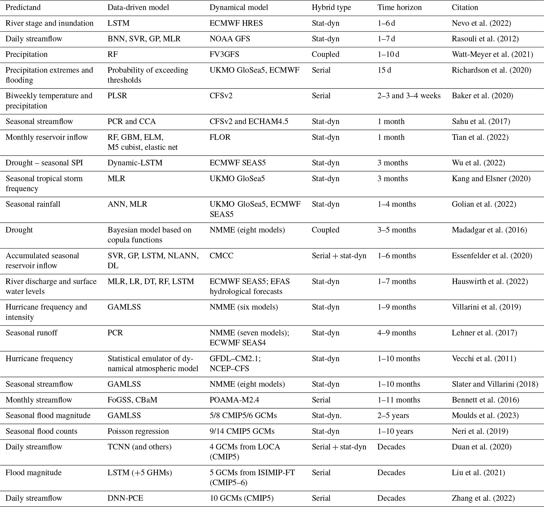
Figure 3Example of a coupled hybrid system for predicting seasonal precipitation several months ahead. (a) Ensemble of precipitation predictions from a dynamical multi-model ensemble such as the NMME. The ribbon indicates the full distribution of model members, and the dark line indicates the mean prediction. (b) Ensemble of statistical precipitation predictions. (c) Both ensembles are overlaid. (d) The two ensembles are blended using a data-driven approach, such as an Expert Advice algorithm, which assigns weights to the different ensemble members based on their performance during training and computes the weighted average prediction. The resulting ensemble mean (orange line) outperforms that of the separate dynamical and statistical predictions. Adapted from Madadgar et al. (2016).
2.2.2 Serial hybrid forecasts that include a hydrological model
Hybrid forecasting systems that include a conceptual hydrological model try to combine the strengths of data-driven and conceptual models, driven with dynamical predictions. For instance, Humphrey et al. (2016) used a combination of historical observations and downscaled dynamical forecasts of rainfall and potential evapotranspiration in southern Australia from POAMA (Predictive Ocean Atmosphere Model for Australia) to drive the conceptual rainfall–runoff model GR4J (Perrin et al., 2003). The simulated soil moisture from GR4J was separately used to drive a Bayesian ANN model to predict streamflow (hybrid approach). They showed that the hybrid model performed better than either the GR4J model or the Bayesian neural network alone. A number of studies have coupled conceptual models and data-driven models but without necessarily integrating dynamical weather or climate predictions (this would be the next step in developing a hybrid forecasting system). Both Anctil et al. (2004) and Kumanlioglu and Fistikoglu (2019) replaced the routing component of the GR4J model with an ANN to predict streamflow in catchments in France, the USA, and the Republic of Türkiye. These studies concluded that the hybrid model was superior to a purely ML model. Other conceptual hydrological models have also been used in hybrid frameworks. For example, Mohammadi et al. (2021) used two conceptual models, HBV (Bergström, 1976) and NRECA (Crawford and Thurin, 1981), to provide inputs to support vector machines (SVMs) and an adaptive neuro-fuzzy inference system (ANFIS), to build seven variants of hybrid models. They tested and compared the hybrids and the individual models (HBV, NRECA, SVMs, and ANFIS) on four subbasins of the Pemali–Comal River basin, Indonesia, and again found the hybrid models performed best in terms of RMSE, R2, and MAE. Other studies on hybrid modelling using the HBV model include Nilsson et al. (2006) and Ren et al. (2018). They both used different variables computed by HBV (e.g. soil moisture and snowmelt) as inputs to ANNs. Okkan et al. (2021) outline that, in most hybrid modelling frameworks, variables computed by the conceptual model are used as inputs to a data-driven model, which necessarily increases computation time. They also note that although there could potentially be interactions between the parameters of the conceptual models and those of the data-driven model, those interactions often go unaccounted for because the two models are calibrated separately. In the context of monthly rainfall–runoff modelling, they proposed to address these two common shortcomings of hybrid models by coupling the two models and performing their calibration jointly.
2.3 Coupled or parallel hybrid models
In the case of coupled hybrid models, a data-driven model and a physics-based model can be run in parallel, sometimes replacing a component of the dynamical model with a data-driven model or combining different types of model predictions. Madadgar et al. (2016) combined the seasonal precipitation predictions from an ensemble of dynamical models (99 members from the NMME) with the precipitation predictions from a statistical model (using copulas to describe the relationship between three large-scale climate indices and precipitation). They used an Expert Advice algorithm to link the dynamical and statistical predictions to obtain improved precipitation predictions over the southwestern USA, as illustrated in Fig. 3.
Coupled hybrid models can also employ a data-driven model to combine other types of dynamical predictions in parallel, such as dynamical meteorological and hydrological predictions. In southern Switzerland, five ML models were trained to predict monthly total hydropower production by combining precipitation, temperature, radiation, and wind speed forecasts from a dynamical meteorological model with runoff from a conceptual hydrological model (Bogner et al., 2019). Day of the week and holiday information were provided to the ML models as additional information to further enhance the prediction.
A third example of a coupled hybrid approach is when data-driven models are employed during the dynamical climate model simulations to correct model biases (e.g. Watt-Meyer et al., 2021). A RF model coupled to an atmospheric model (FV3GFS) can correct temperature, specific humidity, and horizontal winds at each time step, bringing the coupled model in line with observations. This was shown to reduce annual mean precipitation biases by around 20 %, with particular improvements in the simulation of rainfall over high mountains (Watt-Meyer et al., 2021). A similar approach was used by Bretherton et al. (2022) to nudge the output of a low-resolution climate model towards the coarsened output of a high-resolution climate model.
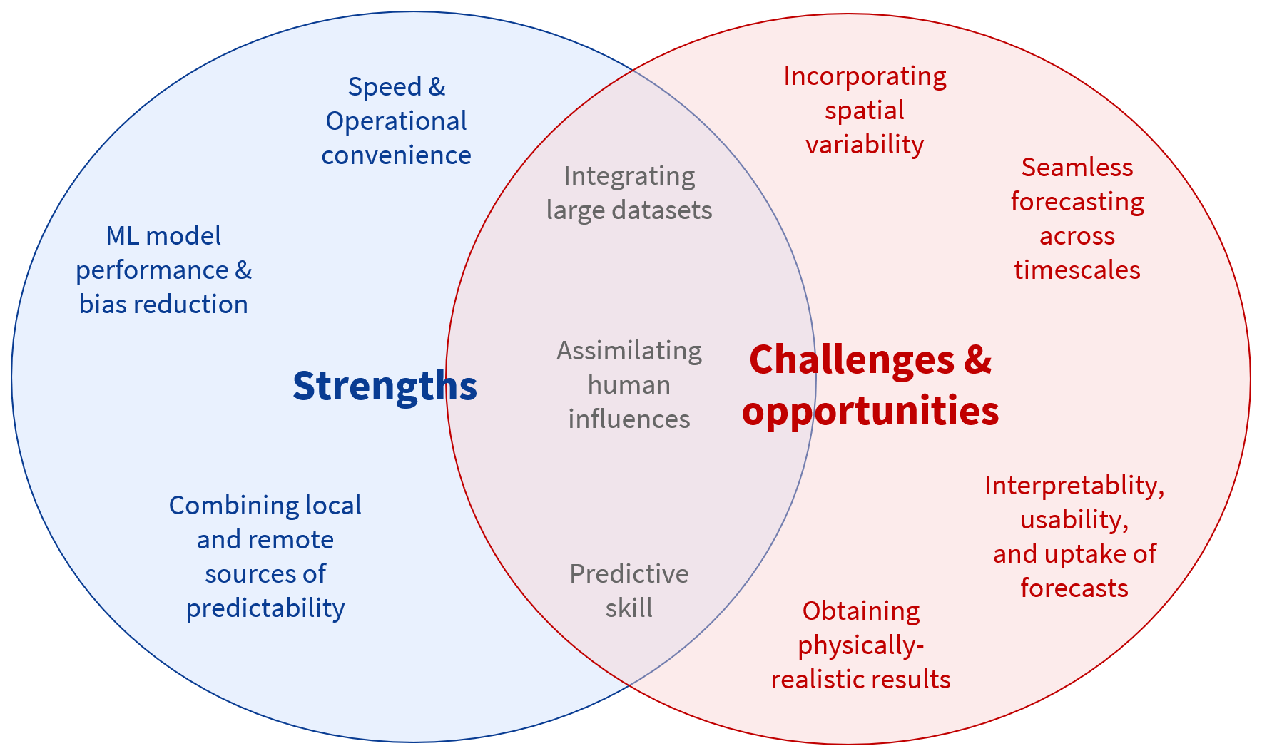
Hybrid methods offer various strengths, as summarized in Fig. 4. These strengths include the higher performance of ML models (in terms of bias and error minimization) and the ability to easily blend outputs from climate multi-model ensembles, integrate large datasets, and combine multiple sources of predictability, as well as improved speed and operational convenience. These strengths are discussed in more detail below.
3.1 ML model performance and bias minimization
Recent work has demonstrated the ability of ML models to outperform traditional hydrological models (e.g. Fang et al., 2017; Kratzert et al., 2019b; Feng et al., 2020; Fang and Shen, 2020a; Lees et al., 2021). In one of the most comprehensive studies to date, Mai et al. (2022) compared 13 locally and globally calibrated models (including ML, lumped, and gridded models) in terms of their ability to simulate streamflow, actual evapotranspiration, surface soil moisture, and snow water equivalent in the Great Lakes region. They found that the ML model outperformed the traditional hydrological models in all experiments. This finding extends to ungauged catchments. Kratzert et al. (2019a) found that an out-of-sample LSTM performed better than the calibrated SAC-SMA (the conceptual model used by the U.S. River Forecast Centers) and the NWM, which is less calibrated. Golian et al. (2021) found that RFs worked best at regionalizing the parameters of the GR6J conceptual model for low-flow prediction in ungauged Irish catchments. Such work has shown the potential of hybrid methods to address the long-standing hydrological challenge of prediction in ungauged basins (e.g. Sivapalan, 2003). The next step is to move from simulation to prediction.
Hybrid models combining ML and climate predictions also tend to outperform the raw dynamical forecasts from climate models. Wu et al. (2022), for instance, developed a hybrid drought-forecasting model of the 3-month Standardized Precipitation Index (SPI). They used RF models to post-process ECMWF SEAS5 predictions of geopotential height, sea level pressure, and air temperature and supplied the output to an LSTM model to predict the 3-month SPI. They found that the SPI predictions from these hybrid models outperformed the predictions of SPI obtained from the raw model outputs. For prediction purposes, hybrid models have the advantage of being able to minimize biases that exist within GCM outputs or that might be otherwise introduced within a hydrological modelling chain. By training a hybrid model directly on the climate model forecasts, rather than on observations, the biases are automatically accounted for within the model (e.g. Slater and Villarini, 2018). This approach is similar to that of model output statistics (MOSs) long used by the weather forecasting community (Glahn and Lowry, 1972) and in seasonal hydrological predictions (Schick et al., 2018). For instance, if a climate model tends to overpredict winter rainfall, then this bias is accounted for directly in the streamflow predictions, given that the model is trained using the same winter rainfall forecasts (assuming a constant bias).
Hybrid models may benefit from a wide range of statistical advances for enhancing the skill of hydroclimate predictions. Since a hybrid system is based on a data-driven model, it is straightforward to incorporate statistical upgrades, such as ensembling the outputs of multiple climate or Earth system models (Duan et al., 2019). One such example is the addition of an error model onto Ensemble Streamflow Prediction (ESP) forecasts to enable prediction in ephemeral rivers (Bennett et al., 2021b). In a hybrid system, one may easily integrate the predictions from multi-model ensembles with over 50 or 100 model members as covariates (Gibson et al., 2021; Slater and Villarini, 2018). Increasing the number and diversity of climate models included within a hydrological predictive model enhances confidence in the hydrological model spread. By blending multi-model ensembles intelligently, one can further reduce uncertainty. In a hybrid system, for instance, one can incorporate time-varying weights for the dynamical predictions, such as Bayesian updating, which varies the model weight per month and lead time (Slater et al., 2017). ML models especially can learn space–time variable input weighting directly (Kratzert et al., 2021). Similarly, many post-processing methods can be applied to weather and climate inputs or the hydrological outputs to enhance skill (Monhart et al., 2019; Bogner et al., 2022).
3.2 Combining local and remote sources of predictability with varying time horizons
One under-researched but promising aspect of hybrid models is their ability to combine different sources of predictability over a continuum of time horizons. Hybrid models can easily make use of different predictors chosen on a sound physical basis (such as climate indices, precipitation, air pressure, and snowfall) without explicitly describing the processes and equations. This makes it much easier to explore information from new sources and improve models and has the potential to widen information access to climate-affected populations. Including additional inputs can also produce marked improvements in model quality. Chang et al. (2022) used seven weather regime indices (based on the 500 hPa geopotential height) with a Gaussian process ML model to post-process subseasonal hydrological forecasts, alongside runoff, soil moisture, baseflow, and snowmelt in Switzerland. The results showed that the additional input of weather regime indices improved the forecast skill, especially in the mountainous catchments and over longer lead times, where skill was difficult to improve without any additional information. The conceptual hydrological model would not have been able to take weather regime indices as input, but by including them in the post-processing ML model as part of the hybrid set-up, it was possible to explore the connection between large-scale weather regimes and local hydrological conditions to improve the forecast skill.
As multiple predictor variables can be included within a statistical or ML model, it is feasible to combine predictors that have very different time-varying impacts, such as reservoir management decisions or initial hydrological conditions impacting the short term, versus annual-to-multi-decadal climate oscillations for longer-term predictability. For instance, Tian et al. (2022) present a reservoir inflow forecasting framework combining a suite of different ML models (including gradient-boosting machine, random forests, and elastic net) with climate model outputs from the FLOR model for reservoirs in the Upper Colorado River basin. They also included soil moisture and evaporation to represent antecedent conditions, which significantly improved the forecasts of reservoir inflow. Ouyang et al. (2021) used a dataset of > 3000 basins across the USA and found that basins with small and medium reservoirs behaved differently from the reference basins but could be well simulated by a LSTM model with input attributes describing basin-lumped reservoir statistics.
Large-scale climate indices or modes can also be combined with other predictors. For instance, Madadgar et al. (2016) predicted seasonal precipitation using large-scale climate indices, namely the PDO, the MEI, and the AMO, computed from outputs of the 99 ensemble members of the NMME. The approach enhanced the skill of the seasonal forecasts by 5 %–60 % in comparison with the raw NMME precipitation forecasts, especially for negative rainfall anomalies. Similarly, Rasouli et al. (2012) forecasted daily streamflow in a river catchment 1–7 d ahead by employing weather forecasts from the NOAA GFS model within a variety of machine learning models. They combined observations with the model outputs and a range of large-scale climate indices representing ENSO, the Pacific–North American teleconnection pattern (PNA), the Arctic Oscillation (AO), and the North Atlantic Oscillation (NAO). Last, Li et al. (2022) used forecasts of the intraseasonal oscillation (ISO), an important mode of subseasonal predictability for seasonal rainfall, to force a Bayesian hierarchical model predicting subseasonal precipitation during the boreal summer monsoon season in different regions of China.
Given the diversity of potential inputs to hybrid forecasting systems, exploratory data analysis to identify correlations between hydrologic variables and climate patterns over different time horizons is an important step during model development. Hagen et al. (2021) employed ML to identify the most relevant large-scale climate indices for daily streamflow forecasting. They provided an overview of studies that have employed large-scale climate indices and climate variables (such as sea level pressure, sea surface temperature, and specific and relative humidity) within ML models for daily, monthly, and seasonal streamflow modelling. Beyond the use of pre-defined climate indices, it is possible to identify tailored, site-specific climate indices from big data and incorporate them in the modelling chain. For instance, Renard and Thyer (2019) described a method that avoids relying on standard climate indices and instead suggests that the most relevant climate indices in a given location are effectively unknown (they are hidden) and can be estimated directly from observations. The authors used a Bayesian hierarchical model for flood occurrence, with hidden climate indices treated as latent variables. They identified the hidden climate indices and then showed their correlation with atmospheric climate variables (geopotential height, zonal westerly wind, and also more distant teleconnections using convective available potential energy and meridional wind). These indices explain the occurrence of flood-rich and flood-poor periods in the historical record. Such an approach could be employed using climate model outputs to develop skilful hybrid forecasts.
Related to the different time horizons of the predictors is also the ability to design hybrid forecasting systems which dynamically update when new information (e.g. observations or climate hindcasts) becomes available. For instance, a statistical model can be updated iteratively over time to track the evolution of nonstationary predictor–predictand relationships. Such approaches incorporate new observations as they become available and update the model parameters (e.g. Slater et al., 2019). Nearing et al. (2022) developed a data assimilation approach for LSTM models that leverages tensor network gradients to assimilate real-time observation data. To date, very little has been published using such methods.
3.3 Integrating large datasets
One perceived challenge of hybrid approaches is the requirement for large numbers of training data to constrain models compared with physics-based or conceptual models. Previously, it was felt that the information requirement of data-driven approaches might hinder their applicability in catchments with limited data (e.g. ungauged basins). Although this might have been true in the past, the increasing availability of large-scale hydroclimatic datasets, such as remote sensing data, is turning this potential challenge into a new opportunity. A data-driven model can be trained on the same data as a conceptual model and will tend to outperform physics-based models, on average (and even more so with large datasets; see Fang et al., 2022). This advantage is partly due to the fact that data-driven models are unconstrained by mass and energy balance rules that force process models to compensate for erroneous inputs, which data-driven models can instead optimize against. Data-driven models learn process relationships and model structures rather than enforce prescribed ones, which may make them more flexible and generalizable. Large training datasets tend to be useful for ML but less so for physics-based models, for these reasons. The ability to leverage large datasets effectively is a strength of ML and in particular for ungauged basins, where several studies have shown that ML models tend to have higher accuracy, on average, than physics-based models calibrated in gauged basins (e.g. Kratzert et al., 2019a). There is, in fact, a data synergy effect, where data of greater diversity lead to better models, according to a systematic study of LSTM models for either streamflow or soil moisture (Fang et al., 2022). With conceptual and process-based models, accuracy can be lost when performing regional (as opposed to basin-specific) calibration, and the lack of calibration data typically results in poor-quality predictions (training on longer periods leads to superior results; see Bogner et al., 2022). In contrast, with hybrid models, strong performance can be achieved when training the models on global datasets, and accuracy is gained when performing regional calibration.
Since long (50 year +) hydroclimatic time series data are not available everywhere (Krabbenhoft, 2022), methods are required that can draw on pooled multi-site approaches with similar catchment and climate characteristics (Kratzert et al., 2019a). For instance, Nearing et al. (2021) show a comparison using pooled vs. unpooled data for streamflow estimation and found that the former was better, even for gauged catchments, and allowed for prediction in ungauged catchments. There are, however, few studies combining LSTM methods with climate model forecasts for long-term (subseasonal to decadal) prediction, especially in ungauged catchments. Such models may start to emerge with the growing availability of observational training datasets, such as the national CAMELS datasets (available for the USA, United Kingdom, Chile, Brazil, Australia, and soon France and Switzerland; e.g. Newman et al., 2015; Addor et al., 2017; Coxon et al., 2020) and international Caravan streamflow dataset (Kratzert et al., 2023). However, real-time data are currently still difficult to access for developing predictive models.
One way to circumvent the lack of observational training data and the low predictability of GCMs is by integrating a range of other types of predictors in hybrid models. This may include sources of remotely sensed measurements such as snow, soil moisture, land cover, surface water extent, water storage, or evapotranspiration to provide better information about the initial states (e.g. Jörg-Hess et al., 2015). There are many different global datasets now available that can be drawn on using cloud-based geospatial analysis platforms such as the Google Earth Engine, as was the case for the creation of an open-source community streamflow dataset (Kratzert et al., 2023). Overall, the forecasting landscape is becoming increasingly complex, with a growing number of forecasting systems and datasets potentially overwhelming users. Hybrid forecasting could help to address this challenge, with hybrid workflows providing a set of tools and data that forecasters could mix and match to address their own forecasting needs.
3.4 Speed and operational convenience
A key advantage of statistical or hybrid methods is their speed and computational efficiency. For instance, the calibration of the GloFAS system with an Evolutionary Algorithm (EA) in 2018 required approximately 6 h to calibrate each one of thousands of streamflow stations on a 12-core PC, depending on the number of generations needed before the improvement criterion was met (Hirpa et al., 2018). Training deep learning (DL) models is now orders of magnitude cheaper in terms of the computational expense. For example, it took about 10 h in 2021 to train an ensemble of long short-term memory (LSTM) networks on a single NVIDIA V100 graphics processing unit (GPU) using 2 decades of daily data from 518 basins in the CAMELS-GB dataset (Lees et al., 2021; i.e. about 70 s per basin). This means that training a high-quality DL model for hundreds of basins is feasible using a standard workstation (or even a GPU-enabled laptop with sufficient memory), while calibrating a conceptual or process-based model over hundreds of basins requires either months of runtime or a high-performance computer (HPC) facility. The training time depends on the computing power, number of locations and volume of data involved, compiler, and optimization. While deep learning methods such as LSTMs can take several hours to train (e.g. Lees et al., 2021), they have the significant advantage that one model is trained on multiple sites (although the fitted model can then be fine-tuned to a specific site). A differentiable ML-based parameter learning scheme can be trained on satellite-based soil moisture observations for the entire continental USA with one GPU in under 1 h, but the conventional approach would take a cluster machine of 100 central processing units (CPUs) 2–3 d to calibrate the model (Tsai et al., 2021).
This efficiency has advantages for water managers. In a traditional setting with limited computational resources, water managers need to quickly run different scenarios (Scher et al., 2021). For instance, the UK Met Office Flood Forecasting Centre will produce a reasonable worst case and a best estimate based on the most likely scenario (see Met Office, Environment Agency and Flood Forecasting Centre, 2013) ahead of a flood event (Arnal et al., 2020). Using all available deterministic and ensemble forecast products alongside expert assessment from the chief forecaster, they will decide what the reasonable worst case is likely to be. These outputs are used to inform the flood guidance statement and the Environment Agency then uses these scenarios to run their catchment models (Pilling et al., 2016). The speed of data-driven approaches in comparison with these more traditional, physics-based modelling approaches could prove beneficial for users wishing to run multiple scenarios quickly. Hybrid methods may shorten the traditional forecasting approach by going end to end, potentially skipping out some of the intermediary steps in a conventional modelling chain, such as downscaling, bias correction, and hydrological modelling. This offers significant potential for applications where the run time of physically based models limits the ability to provide forecasts with a useful lead time for action – such as forecasts of pluvial floods Rözer et al. (2021) or flash floods.
The efficiency of hybrid models may also be helpful in generating faster research cycles for model improvements (i.e. setting up an upgraded system and releasing hindcasts for testing) relative to traditional approaches. Model upgrades for dynamical systems usually take a very long time because the model has to be recalibrated and a set of x (e.g. 30) years of hindcast data must be produced to quantify the impact of the changes to the system.
Last, hybrid systems can be used to develop customized climate services. For instance, Essenfelder et al. (2020) use data-driven methods to predict seasonal reservoir inflows for hydropower plants. The information is made easily accessible online to support decision-makers in hydropower production. Such approaches can be designed to be replicated globally as a climate service, provided there are suitable data for training, and by developing transferable rule sets. Bennett et al. (2016, p. 8239) also highlight the importance of operational convenience and the advantages of combining the convenience of stochastic scenarios with the skill of a modern forecasting system. Their method enhances the precipitation forecasts necessary for streamflow forecasting through post-processing – by reducing the biases, correcting the reliability, and maximizing the forecast signal.
Beside the strengths of hybrid methods, there are challenges and research priorities to be tackled. As hybrid forecasts and predictions rely on data-driven models, they inevitably inherit some of the limitations of these techniques. Frequently cited limitations of ML models include the requirement for large datasets and issues associated with the curse of dimensionality, namely data sparsity (i.e. when there are too few data points relative to the number of dimensions), multi-collinearity of the variables, multiple testing (leading to an increased number of false positives), and overfitting (Altman and Krzywinski, 2018). There is also the difficulty of obtaining physically plausible results for previously unseen extremes that are larger than those seen in the observational record; however, new research suggests that ML models may provide results that are more physically plausible than physics-based and conceptual models when data are biased (Frame et al., 2022b). Further challenges for improving the skill of hybrid models include data assimilation, physics-guided ML designs, assimilation of human influences, model optimization, ensembling, and hybridization, where models are merged with other methods (including simulations and physical models; e.g. Mosavi et al., 2018). While some of the difficulties associated with large sample sizes apply less for seasonal to decadal hybrid forecasting, where the sample sizes can be much smaller (often near 100 values) than the sample sizes for shorter ranges (thousands or more), the small sample sizes present a challenge for model training. Thus, a range of different challenges may apply, depending on the forecasting horizon and data required.
4.1 Obtaining physically realistic results
One important challenge of hybrid models is the need to produce physically plausible or explainable forecasts in unseen extreme conditions such as severe floods, droughts, intense heatwaves, and tropical storms. This is particularly important as new weather records are being set in different parts of the world, and models must produce credible predictions under extreme forcing conditions. Although it has sometimes been suggested that data-driven models might be less suited to extrapolation to out-of-sample conditions than physics-based models due to the lack of physical understanding (e.g. Reichstein et al., 2019), recent work tackled the question of whether modern LSTMs could predict events larger than those seen in the training data for a particular catchment. The authors found that the LSTM could predict unseen streamflow extremes and did this better than the physics-based models that were used in the study (Frame et al., 2022a). It is now increasingly recognized that one of the advantages of data-driven models is their flexibility, allowing them to find unexpected patterns in the data. Thus, there are emerging synergies between data-driven and physics-based approaches, since the former can enhance the performance of the latter, e.g. by learning the parameterizations required for the physical models from large datasets or analysing the patterns of error from the physical models (Reichstein et al., 2019).
One emerging route for hybrid models is to employ physics-guided or theory-guided ML designs that explicitly observe the law of conservation of mass. Such approaches seek to integrate physical knowledge within the data-driven models to take advantage of the strengths of both. For instance, Hoedt et al. (2021) created an LSTM architecture that obeys conservation laws, and these laws can also be used to guide physical interpretation of model outcomes. Although there have been considerable methodological advances in interpreting neural networks (e.g. Wilby et al., 2003; Toms et al., 2020; Lees et al., 2022), physics-guided ML approaches (also referred to as physics-informed, physics-aware, or theory-guided approaches) still require further development. As alluded to earlier, the presence of data errors in observed hydroclimate records means that an unconstrained ML performs better than a physics-guided ML model because of the ability to learn and account for data errors (Beven, 2020; Frame et al., 2022b), including heteroscedastic and nonstationary data errors (Kratzert et al., 2021).
Another new development is differentiable, learnable, physics-based models that can not only approach the performance of ML models but also output internal physical variables such as evapotranspiration and soil moisture (Feng et al., 2022b; Shen et al., 2023). Tsai et al. (2021) first demonstrated the ability of connected neural networks to provide physical parameter sets to process-based models. They showed the efficiency and generalizability of this paradigm for untrained variables, spatial extrapolation, and interpretability. In data-sparse regions, this approach can even produce better daily metrics and future trends than LSTM (Feng et al., 2022a) and can be used to improve flood routing (Bindas et al., 2022). These models seek to combine the power of both ML and physics and have the potential to alleviate data demand, extrapolate better in space and for more extreme conditions, and be constrained by multi-variate observations to enable better forecasts. Furthermore, they provide a systematic pathway for asking scientific questions and obtaining answers from big data.
Explainability is sometimes useful to help develop trust in model predictions. Forecasting agencies frequently engage in a form of story-telling, both for internal and external communication. One reason for providing explainable predictions is that, when the forecasts evolve for a given variable, such as spring runoff, users often wish to understand why (i.e. what has changed in the predictors or other factors to explain the change in the predictions). One way to achieve explainability is by providing storylines or narratives around the hybrid forecasts which demonstrate the geophysical credibility of the results. Differentiable modelling can also provide diverse physical variable outputs, trained or untrained, which help develop a narrative (Feng et al., 2022b). Fleming et al. (2021) showed how hydroclimatic storylines can be produced for clients to make the forecast interpretable in terms of understandable geophysical processes. They used pragmatic methods such as popular votes for the candidate predictors cast by a genetic algorithm. The approach revealed how the values of predictors such as antecedent flow and snow water equivalent could help explain the ensemble-mean-predicted volume. However, there are also limitations to such approaches. Although narratives may help with stakeholder acceptance of hybrid forecasting systems, they can also form a constraint on the forecasting approach, by enforcing consistency of a given prediction method.
4.2 Assimilating human influences
Another emerging challenge is assimilating human influences on the water cycle to obtain better predictions of hydroclimate variables, especially droughts (Brunner et al., 2021; Van Loon et al., 2022). Limited data exist on human impacts such as water storage, groundwater depletion, irrigation, land cover changes, and water transfers. Therefore, how can human decisions, such as the management of reservoir levels or flow abstraction, be integrated within hydrological forecasts? This question is especially relevant over longer timescales, and for hydrological forecasting in general, as access to such data is limited (e.g. only very limited information on reservoir operations is included in GloFAS). One option is to develop proxies to detect and model human influence. For instance, census information on the number of households has be used to extend UK urbanization records (Han et al., 2022). Population density data have also been used as a proxy for urbanization, to assess the extent to which seasonal streamflow predictability might benefit from anthropogenic predictors such as land cover change alongside seasonal climate forecasts (Slater and Villarini, 2018). López and Francés (2013) supplied a dynamic reservoir index alongside climate indices to predict historical annual maximum peak discharge in Spanish rivers. In a large-scale study it was found that reservoir operations could be implicitly simulated by ML approaches that learn from past operations (Ouyang et al., 2021). Last, information on the day of the week and on local festivities has been used successfully as a proxy for difference in energy demand (Bogner et al., 2019). Such proxies might also inform a hybrid system on hydro-peaking in rivers downstream of dams.
The lack of accurate predictions of future human activities at the catchment scale is also a major limitation for hydrological forecasting over longer timescales. Here, the increasing coverage and resolution of satellite data may help to provide relevant inputs to hybrid forecasting models such as future predictions of land use change (e.g. Moulds et al., 2015). Emerging satellite altimetry products (e.g. SWOT) may enable a better understanding of reservoir operations, which can be used to constrain hydrological forecasts. Similarly, ML could potentially be used to translate major socioeconomic drivers into land cover change. Overall, we suggest that the main bottleneck to integrating human activities in hybrid forecasting systems is not the model algorithms, which can be adapted to any potential predictors, but rather the lack of consistent historical and future time series data on these activities. Unfortunately, this is likely to be a vexing challenge for automated representation. In many reservoir systems, for instance, operations are determined through unpredictable human interactions and negotiations and may depend on time-varying legal, institutional, ecological, and economic factors, such as agricultural markets influencing irrigation practice, or fisheries health directing environmental releases.
4.3 Developing predictive skill
Dynamical forecasts and predictions tend to have low skill over long lead times. The skill of short-term hydroclimatological forecasts is constrained by the skill of meteorological forecasts, which is currently in the range of 3 to 10 d ahead but has been advancing by about 1 d per decade, such that “today's 6 d forecast is as accurate as the 5 d forecast 10 years ago” (Bauer et al., 2015, p. 47). Low flows may have skill up to 20 d in the case of Fundel et al. (2013) and even longer in other cases, especially with good information on initial conditions and/or the memory effect of catchment storage. Seasonal climate forecasts also have low predictive skill beyond a couple of months, while both seasonal and decadal predictions suffer from the underestimation of atmospheric circulation in climate models, a phenomenon known as the signal-to-noise paradox (e.g. Smith et al., 2020).
One of the advantages of hybrid predictions is that the data-driven methods can be used to enhance predictive skill of the dynamical meteorological or climate forecasts. For instance, decadal predictions are skilful over multi-year forecast periods but have too much uncertainty to provide useful information on interannual variability. Although the CMIP5–6 models can skilfully reproduce certain large-scale circulation patterns, the magnitude of teleconnections tends to be underestimated. Statistical approaches such as NAO-matching attempt to resolve this by selecting members based on their ability to reproduce climate indices and their teleconnections (Smith et al., 2020). Such methods have been employed to enhance decadal streamflow prediction (Moulds et al., 2023) and condition seasonal hydrological forecasts (Donegan et al., 2021). However, further work is still needed to interpret multi-year forecasts to provide actionable information. Given a skilful multi-year forecast, it should be possible to estimate the increased flood or drought risk (for instance) in each year of the forecast period. Data-driven techniques may aid in future developments by trying to draw out the climate model members that perform well in given months or lead times (e.g. Slater et al., 2017).
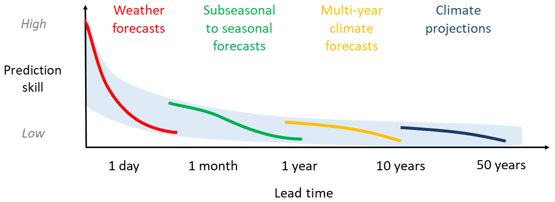
Figure 5Hybrid models could be a promising route for seamlessly linking initialized predictions from seasonal and decadal forecasts to scenario-based projections across timescales. Different ML-based bias correction approaches could be explored for merging or concatenating the covariate time series (e.g. Befort et al., 2022) before using them to drive a hybrid hydroclimate prediction model (e.g. for streamflow). Such an approach is likely to be more challenging for extremes such as floods and droughts and remains an open research question.
4.4 Seamless forecasting: merging forecasts, predictions, and projections
The utility of hybrid models for seamless hydroclimatic prediction systems spanning weeks to decades is an open research question (Fig. 5). There is a growing need for reliable long-term predictions of climate change impacts on the risk of floods and droughts over the coming decades (i.e. 1–40 years ahead), yet reliable information does not exist over such timescales. The lack of seamless climate information is explained by the fact that different scientific weather and climate products have been developed for different applications. Short-term predictions (fewer than 5 years ahead) tend to rely more on correct initial conditions, while long-term predictions and projections (> 10 years ahead) rely more on correct external forcings such as greenhouse gases (Boer et al., 2016).
One way to provide longer-term climate impacts information over the coming decades is to constrain uninitialized climate model projections (e.g. climate simulations for the RCP4.5 or RCP8.5 scenarios) using initialized decadal predictions (such as the CMIP6 decadal hindcasts), which tend to better reflect observed climate variability. Befort et al. (2020) developed a method that does this by selecting the climate projections that best match the mean of the decadal predictions over the next 10 years. They showed that the constrained ensemble, which consisted of uninitialized projections for the upcoming 50 years, had higher skill than the full projection ensemble, even after the 10-year period, once decadal prediction information was no longer available. A hybrid system for enhanced prediction of hydroclimatic impacts (e.g. flood risk) could integrate the outputs of such a constrained ensemble.
Beyond the use of uninitialized projections by themselves (covering the whole 1–50-year period), temporally concatenating a bias-corrected time series of decadal climate predictions and climate projections is also possible. Befort et al. (2022) assessed different types of bias correction and found that the variance inflation (VINF) method could reduce inconsistencies between the decadal- and century-scale time series, especially for central quantiles of the climate time series (close to the multi-model ensemble median). However, the method could not eliminate all inconsistencies, notably those for extreme quantiles. A seamless hybrid method would therefore be more difficult to generate for hydroclimate extremes such as floods and droughts. However, these two papers (Befort et al., 2020, 2022) open the way for novel research on the merging of decadal predictions and uninitialized projections as input to seamless prediction schemes for hydroclimate impacts using hybrid ML-based approaches.
4.5 Incorporating spatial variability
The data employed in many hybrid hydrological models are often lumped, i.e. spatially averaged at the catchment scale, ignoring spatial variability in landscape and atmospheric forcing. Lumped models are challenging for the prediction of hydroclimate in complex environments such as snow-dominated watersheds, which may have karst conduits, or the spatiotemporal variation in snow accumulation and snowmelt processes. However, new approaches exist to overcome this limitation in statistical/machine learning models. For instance, Shi et al. (2015) developed a convolutional LSTM, termed convLSTM, which is able to capture spatiotemporal correlations, considering both the input and the prediction target as spatiotemporal sequences. One example is the use of past and future radar maps as input and output; such spatiotemporal sequences have high dimensionality and, until recently, could not be included in hydroclimate prediction schemes. Similarly, Gupta et al. (2021) developed a spatial variability aware neural network, termed SVANN-E, in which the architecture of the neural network varied spatially across geographic locations. They evaluated the approach using high-resolution imagery for wetland mapping. Such novel spatiotemporal prediction approaches are just starting to be used for hydroclimate prediction. Xu et al. (2022) used a hybrid approach to predict streamflow in a watershed with spatially variable karst carbonate bedrock. They combined a spatially distributed snow model with a deep learning karst model based on convLSTM, which simulated the effect of surface and subsurface properties on the streamflow. This approach allowed the authors to better include the spatial variability in the input variables to their prediction scheme.
4.6 Interpretability, usability, and uptake of hybrid forecasts
Hybrid approaches for hydroclimate prediction over subseasonal to decadal lead times face several challenges to their continued uptake by various communities. One issue that is critical to making hybrid schemes more widely accepted is determining whether the improvement in forecast skill obtained by building a hybrid model is worth the extra effort. In other words, it can be difficult to determine a priori how much added value can be obtained without first developing the hybrid model and benchmarking the results against a more traditional approach. Despite a commitment to developing the use of ML within operational hydrology (e.g. Environment Agency, 2022), close co-operation is needed between the hydrology, forecasting, and ML communities to explore their potential either alone or in hybrid frameworks (Mosavi et al., 2018), build trust (Haupt et al., 2022), communicate skill (Thielen-del Pozo and Bruen, 2019), and overcome barriers to operational uptake (Speight et al., 2021). The benchmarking study of Mai et al. (2022) provided a detailed intercomparison of modelling approaches over the Great Lakes region (USA and Canada), suggesting that the effort related to ML is justifiable. However, this work was for retrospective simulation, rather than forecasting (for which there are more steps needed), and research is still needed to assess ML's potential for improving prediction skill, particularly over seasonal to decadal horizons, for which studies are lacking. In the hybrid set-up of Humphrey et al. (2016), for instance, which required the development of both an ML and a conceptual model for three gauges in southern Australia, the authors found that the hybrid model was more skilful than either the conceptual or the data-driven models alone. However, the increase in skill was only marginal for one of the three study locations. They concluded that for this given station, the extra time and effort required to implement the hybrid model was not worth the small gains. Implementing an operational hybrid framework for hydroclimatic forecasting often requires extensive time and expertise, given that two completely different types of models must be developed in parallel. These requirements would also likely require a shift in the expertise of the organization in addition to an upgrade in the computing architecture in the case of GPU-requiring hybrid and data-driven approaches. Overall, the operational uptake of hybrid models is expected to be faster in cases where there is no existing forecasting capability (requiring modification) or where complex physical processes make traditional approaches challenging.
Hybrid forecasting is emerging as a powerful enhancement to traditional hydroclimatic forecasting techniques, but important questions remain regarding their place in the pantheon of methods. We lay out some of the most important research possibilities. First are questions about the evaluation of hybrid methods. How well do dynamical-statistical methods perform when compared with more traditional, operational approaches? What benchmarks should be used? How reliable are these models, and over what lead times can they be trusted? As far as we are aware, there have been very few papers (if any) comparing the skill of hybrid models with operational systems. One systematic comparison of 13 different models (including machine-learning-based, basin-wise, subbasin-based, and gridded models) revealed the superiority of the data-driven LSTM-lumped model in all experiments (e.g. Mai et al., 2022), suggesting that hybrid LSTM-based prediction systems would be a promising route for daily simulation and potentially for applications such as forecasting.
Second are questions about the potential for seamless prediction. To what extent can hybrid approaches be employed to meld historical trends, near-term, and decadal predictions of hydroclimate variables from atmospheric forecasts, climate model predictions, and projections? How would such a system be used operationally? Seamless hybrid prediction may provide better insights into long-term hydroclimatic trends, but merging across timescales can lead to inconsistencies in the time series (i.e. jumps or step changes) between, for example, decadal climate predictions and the climate projections (Befort et al., 2022). Third are questions about using data-driven models to detect and attribute the drivers of hydrologic change (Slater et al., 2021), and then integrating such knowledge within a predictive framework. How can data-driven approaches be employed to understand the relative contributions of different predictors, including human impacts such as the effects of reservoir regulation on streamflow (Brunner and Naveau, 2023)? To what extent can hybrid models uncover hidden large-scale climatic or anthropogenic drivers of change (Renard et al., 2022; Lees et al., 2022)?
An important step forward would be the development of consistent global datasets of climate hindcasts at various timescales at the catchment level. Similar datasets developed for large sample hydrological analyses, such as CAMELS (e.g. Addor et al., 2017; Coxon et al., 2020) and Caravan (Kratzert et al., 2023), have driven rapid progress in ML methods for simulating daily streamflow using observed climate inputs. Such datasets drive progress towards operational hybrid systems by making it easier for model developers to train and test potential methods in a pseudo-operational context. Moreover, they could integrate consistent estimates of other potential drivers – including streamflow signatures and local characteristics related to topography, geology, and land cover (as in the CAMELS datasets) – enabling forecasters to understand the contribution of different drivers to streamflow predictability across timescales.
Finally, there are questions about the acceptance and viability of hybrid models in operational contexts, given the dominance, familiarity with, and deep embedding of physics-based forecasting and prediction methods (Cohen et al., 2019). In what ways could hybrid approaches complement, support, or replace conventional physically based systems? The pace of change in such settings is often constrained by practicalities, institutional resistance (Arnal et al., 2020), or the requirement for decision-relevant evidence of skill. Acceptance might be advanced by systematically comparing the outputs from hybrid models with operational models under identical forcings to assess the physical interpretation of model results (e.g. Mai et al., 2022). To convince operational forecasters that hybrid models may add value alongside more traditional approaches requires rigorous benchmarking by the community alongside established approaches. It may also require more extensive changes to the education and preparation of the workforce that is needed to staff operational centres.
There are several possible paths forward. One of these frames hybrid models not as replacing current operational systems but as a complementary tool, extension, or enhancement, helping on different levels and likely within existing systems. Another path forward is to recognize the difference in skill between hybrid models vs. traditional models and to start to develop future replacements for current operational models. These replacements should be based fundamentally on data-driven (ML, DL, and even AI) principles but with the ability to incorporate elements of traditional hydrological and climate science where these are beneficial. Furthermore, hybrid models could be developed to estimate both impacts and mitigation measures based on past events. All of these approaches make sense for different reasons and in different scenarios, and various agencies and organizations are pursuing both these and other strategies for incorporating data-driven methods into operational workflows. Overall, the utility of hybrid models is not only for enhancing forecasting and prediction but also for allowing deeper interrogation of diverse data, revealing sometimes hidden or obscure hydroclimatological processes.
No data sets were used in this article.
LJS conceptualized the paper and wrote the original draft. LJS, LA, and AYC produced the visualizations. LA, MB, AYC, SM, CM, GN, GS, CS, LS, GV, RLW, AW, and MZ contributed to the conceptualization of ideas and to the writing and editing of the manuscript.
At least one of the (co-)authors is a member of the editorial board of Hydrology and Earth System Sciences. The peer-review process was guided by an independent editor, and the authors also have no other competing interests to declare.
Publisher's note: Copernicus Publications remains neutral with regard to jurisdictional claims in published maps and institutional affiliations.
We wish to thank two anonymous reviewers for their insightful comments that helped improve the work.
This research has been supported by the UK Research and Innovation (grant nos. MR/V022008/1 and NE/S015728/1), the Swiss Federal Institute for Forest, Snow and Landscape Research (MaLeFix; Extremes), the Canada First Research Excellence Fund (Global Water Futures programme), the U.S. Army Corps of Engineers (USACE Institute for Water Resources), and the Science Foundation Ireland (grant no. SFI/17/CDA/4783).
This paper was edited by Nadav Peleg and reviewed by two anonymous referees.
Addor, N., Newman, A. J., Mizukami, N., and Clark, M. P.: The CAMELS data set: catchment attributes and meteorology for large-sample studies, Hydrol. Earth Syst. Sci., 21, 5293–5313, https://doi.org/10.5194/hess-21-5293-2017, 2017. a, b
AghaKouchak, A., Pan, B., Mazdiyasni, O., Sadegh, M., Jiwa, S., Zhang, W., Love, C. A., Madadgar, S., Papalexiou, S. M., Davis, S. J. and Hsu, K: Status and prospects for drought forecasting: opportunities in artificial intelligence and hybrid physical–statistical forecasting, Philos. T. R. Soc. A, 380, 20210288, 2022. a, b
Alfieri, L., Burek, P., Dutra, E., Krzeminski, B., Muraro, D., Thielen, J., and Pappenberger, F.: GloFAS – global ensemble streamflow forecasting and flood early warning, Hydrol. Earth Syst. Sci., 17, 1161–1175, https://doi.org/10.5194/hess-17-1161-2013, 2013. a
Altman, N. and Krzywinski, M.: The curse(s) of dimensionality, Nat. Methods, 15, 399–400, 2018. a
Anctil, F., Michel, C., Perrin, C., and Andréassian, V.: A soil moisture index as an auxiliary ANN input for stream flow forecasting, J. Hydrol., 286, 155–167, 2004. a
Anderson, G. J. and Lucas, D. D.: Machine Learning Predictions of a Multiresolution Climate Model Ensemble, Geophys. Res. Lett., 45, 4273–4280, https://doi.org/10.1029/2018GL077049, 2018. a
Arheimer, B., Pimentel, R., Isberg, K., Crochemore, L., Andersson, J. C. M., Hasan, A., and Pineda, L.: Global catchment modelling using World-Wide HYPE (WWH), open data, and stepwise parameter estimation, Hydrol. Earth Syst. Sci., 24, 535–559, https://doi.org/10.5194/hess-24-535-2020, 2020. a
Arnal, L., Cloke, H. L., Stephens, E., Wetterhall, F., Prudhomme, C., Neumann, J., Krzeminski, B., and Pappenberger, F.: Skilful seasonal forecasts of streamflow over Europe?, Hydrol. Earth Syst. Sci., 22, 2057–2072, https://doi.org/10.5194/hess-22-2057-2018, 2018. a, b
Arnal, L., Anspoks, L., Manson, S., Neumann, J., Norton, T., Stephens, E., Wolfenden, L., and Cloke, H. L.: “Are we talking just a bit of water out of bank? Or is it Armageddon?” Front line perspectives on transitioning to probabilistic fluvial flood forecasts in England, Geoscience Communication, 3, 203–232, 2020. a, b
Baker, S., Wood, A., and Rajagopalan, B.: Application of Postprocessing to Watershed-Scale Subseasonal Climate Forecasts over the Contiguous United States, J. Hydrometeorol., 21, 971–987, https://doi.org/10.1175/JHM-D-19-0155.1, 2020. a, b
Bauer, P., Thorpe, A., and Brunet, G.: The quiet revolution of numerical weather prediction, Nature, 525, 47–55, 2015. a
Befort, D., Brunner, L., Borchert, L., O'Reilly, C., Mignot, J., Ballinger, A., Hegerl, G., Murphy, J., and Weisheimer, A.: Combination of decadal predictions and climate projections in time: Challenges and potential solutions, Geophys. Res. Lett., 49, e2022GL098568, https://doi.org/10.1029/2022GL098568, 2022. a, b, c, d
Befort, D. J., O'Reilly, C. H., and Weisheimer, A.: Constraining projections using decadal predictions, Geophys. Res. Lett., 47, e2020GL087900, https://doi.org/10.1029/2020GL087900, 2020. a, b
Bennett, J. C., Wang, Q., Li, M., Robertson, D. E., and Schepen, A.: Reliable long-range ensemble streamflow forecasts: Combining calibrated climate forecasts with a conceptual runoff model and a staged error model, Water Resour. Res., 52, 8238–8259, 2016. a, b, c
Bennett, J. C., Robertson, D. E., Wang, Q. J., Li, M., and Perraud, J.-M.: Propagating reliable estimates of hydrological forecast uncertainty to many lead times, J. Hydrol., 603, 126798, https://doi.org/10.1016/j.jhydrol.2021.126798, 2021a. a
Bennett, J. C., Wang, Q., Robertson, D. E., Bridgart, R., Lerat, J., Li, M., and Michael, K.: An error model for long-range ensemble forecasts of ephemeral rivers, Adv. Water Resour., 151, 103891, https://doi.org/10.1016/j.advwatres.2021.103891, 2021b. a
Bergström, S.: Development and application of a conceptual model for Scandinavian catchments, Tech. Rep. Report RHO No. 7, Norrköping, Sweden, 1976. a
Beven, K.: Deep learning, hydrological processes and the uniqueness of place, Hydrol. Process., 34, 3608–3613, 2020. a
Bindas, T., Tsai, W.-P., Liu, J., Rahmani, F., Feng, D., Bian, Y., Lawson, K., and Shen, C.: Improving large-basin streamflow simulation using a modular, differentiable, learnable graph model for routing, Authorea, 29 September 2022, https://doi.org/10.1002/essoar.10512512.1, 2022. a
Bisson, J. and Roberge, F.: Prévision des apports naturels: Expérience d'Hydro-Québec, workshop on flow predictions, in: IEEE Institute of Electrical and Electronics Engineers, November 1983, Toronto, 1983. a
Boer, G. J., Smith, D. M., Cassou, C., Doblas-Reyes, F., Danabasoglu, G., Kirtman, B., Kushnir, Y., Kimoto, M., Meehl, G. A., Msadek, R., Mueller, W. A., Taylor, K. E., Zwiers, F., Rixen, M., Ruprich-Robert, Y., and Eade, R.: The Decadal Climate Prediction Project (DCPP) contribution to CMIP6, Geosci. Model Dev., 9, 3751–3777, https://doi.org/10.5194/gmd-9-3751-2016, 2016. a
Bogner, K., Pappenberger, F., and Zappa, M.: Machine Learning Techniques for Predicting the Energy Consumption/Production and Its Uncertainties Driven by Meteorological Observations and Forecasts, Sustainability, 11, 3328, https://doi.org/10.3390/su11123328, 2019. a, b, c
Bogner, K., Chang, A. Y., Bernhard, L., Zappa, M., Monhart, S., and Spirig, C.: Tercile Forecasts for Extending the Horizon of Skillful Hydrological Predictions, J. Hydrometeorol., 23, 521–539, https://doi.org/10.1175/JHM-D-21-0020.1, 2022. a, b, c
Bretherton, C. S., Henn, B., Kwa, A., Brenowitz, N. D., Watt-Meyer, O., McGibbon, J., Perkins, W. A., Clark, S. K., and Harris, L.: Correcting Coarse-Grid Weather and Climate Models by Machine Learning From Global Storm-Resolving Simulations, J. Adv. Model. Earth Sy., 14, e2021MS002794, https://doi.org/10.1029/2021MS002794, 2022. a
Brunner, M. I. and Naveau, P.: Spatial variability in Alpine reservoir regulation: deriving reservoir operations from streamflow using generalized additive models, Hydrol. Earth Syst. Sci., 27, 673–687, https://doi.org/10.5194/hess-27-673-2023, 2023. a
Brunner, M. I., Slater, L., Tallaksen, L. M., and Clark, M.: Challenges in modeling and predicting floods and droughts: A review, Wiley Interdisciplin. Rev.: Water, 8, e1520, https://doi.org/10.1002/wat2.1520, 2021. a
Burnash, R. J., Ferral, R. L., and McGuire, R. A.: A generalized streamflow simulation system: Conceptual modeling for digital computers, US Department of Commerce, National Weather Service, and State of California, Department of Water Resource, 1973. a
Cao, J., Wang, H., Li, J., Tian, Q., and Niyogi, D.: Improving the Forecasting of Winter Wheat Yields in Northern China with Machine Learning–Dynamical Hybrid Subseasonal-to-Seasonal Ensemble Prediction, Remote Sens.-Basel, 14, 1707, 2022. a
Chang, A. Y., Bogner, K., Grams, C. M., Monhart, S., Domeisen, D. I., and Zappa, M.: Exploring the use of European weather regimes for improving user-relevant hydrological forecasts at the sub-seasonal scale in Switzerland, J. Hydrometeorol., in review, 2022. a
Cohen, J., Coumou, D., Hwang, J., Mackey, L., Orenstein, P., Totz, S., and Tziperman, E.: S2S Reboot: An Argument for Greater Inclusion of Machine Learning in Subseasonal to Seasonal Forecasts, WIREs Climate Change, 10, e00567, https://doi.org/10.1002/wcc.567, 2019. a, b
Coxon, G., Addor, N., Bloomfield, J. P., Freer, J., Fry, M., Hannaford, J., Howden, N. J. K., Lane, R., Lewis, M., Robinson, E. L., Wagener, T., and Woods, R.: CAMELS-GB: hydrometeorological time series and landscape attributes for 671 catchments in Great Britain, Earth Syst. Sci. Data, 12, 2459–2483, https://doi.org/10.5194/essd-12-2459-2020, 2020. a, b
Crawford, N. and Thurin, S.: Hydrologic estimates for small hydroelectric projects. Small Decentralized Hydropower Program, International Programs Division, National Rural Electric Cooperative Association, Washington, DC, USA, 1981. a
DelSole, T. and Shukla, J.: Artificial skill due to predictor screening, J. Climate, 22, 331–345, 2009. a, b
Dixon, S. G. and Wilby, R. L.: A seasonal forecasting procedure for reservoir inflows in Central Asia, River Res. Appl., 35, 1141–1154, 2019. a
Donegan, S., Murphy, C., Harrigan, S., Broderick, C., Foran Quinn, D., Golian, S., Knight, J., Matthews, T., Prudhomme, C., Scaife, A. A., Stringer, N., and Wilby, R. L.: Conditioning ensemble streamflow prediction with the North Atlantic Oscillation improves skill at longer lead times, Hydrol. Earth Syst. Sci., 25, 4159–4183, https://doi.org/10.5194/hess-25-4159-2021, 2021. a
Duan, Q., Pappenberger, F., Wood, A., Cloke, H. L., and Schaake, J.: Handbook of hydrometeorological ensemble forecasting, vol. 845, Springer, Berlin, Heidelberg, Germany, ISBN 978-3-642-39924-4, 2019. a
Duan, S., Ullrich, P., and Shu, L.: Using convolutional neural networks for streamflow projection in california, Front. Water, 2, Frontiers in Water, 2, 28, https://doi.org/10.3389/frwa.2020.00028, 2020. a, b
Emerton, R., Zsoter, E., Arnal, L., Cloke, H. L., Muraro, D., Prudhomme, C., Stephens, E. M., Salamon, P., and Pappenberger, F.: Developing a global operational seasonal hydro-meteorological forecasting system: GloFAS-Seasonal v1.0, Geosci. Model Dev., 11, 3327–3346, https://doi.org/10.5194/gmd-11-3327-2018, 2018. a
Environment Agency: Flood Hydrology Roadmap: Roadmap development and the action plan (FRS18196/R1), Tech. rep., https://assets.publishing.service.gov.uk/media/62335ac2e90e070a54e18185/FRS18196_Flood_hydrology_roadmap_-_report.pdf (last access: 6 May 2023), 2022. a
Essenfelder, A. H., Larosa, F., Mazzoli, P., Bagli, S., Broccoli, D., Luzzi, V., Mysiak, J., Mercogliano, P., and dalla Valle, F.: Smart Climate Hydropower Tool: A Machine-Learning Seasonal Forecasting Climate Service to Support Cost–Benefit Analysis of Reservoir Management, Atmosphere, 11, 1305, https://doi.org/10.3390/atmos11121305, 2020. a, b, c
Fang, K. and Shen, C.: Near-Real-Time Forecast of Satellite-Based Soil Moisture Using Long Short-Term Memory with an Adaptive Data Integration Kernel, J. Hydrometeorol., 21, 399–413, https://doi.org/10.1175/JHM-D-19-0169.1, 2020a. a
Fang, K. and Shen, C.: Near-real-time forecast of satellite-based soil moisture using long short-term memory with an adaptive data integration kernel, J. Hydrometeorol., 21, 399–413, 2020b. a
Fang, K., Shen, C., Kifer, D., and Yang, X.: Prolongation of SMAP to spatiotemporally seamless coverage of continental U. S. using a deep learning neural network, Geophys. Res. Lett., 44, 11030–11039, 2017. a
Fang, K., Kifer, D., Lawson, K., Feng, D., and Shen, C.: The Data Synergy Effects of Time-Series Deep Learning Models in Hydrology, Water Resour. Res., 58, e2021WR029583, https://doi.org/10.1029/2021WR029583, 2022. a, b
Feng, D., Fang, K., and Shen, C.: Enhancing Streamflow Forecast and Extracting Insights Using Long-Short Term Memory Networks With Data Integration at Continental Scales, Water Resour. Res., 56, e2019WR026793, https://doi.org/10.1029/2019WR026793, 2020. a, b
Feng, D., Lawson, K., and Shen, C.: Mitigating Prediction Error of Deep Learning Streamflow Models in Large Data-Sparse Regions With Ensemble Modeling and Soft Data, Geophys. Res. Lett., 48, e2021GL092999, https://doi.org/10.1029/2021GL092999, 2021. a, b
Feng, D., Beck, H., Lawson, K., and Shen, C.: The suitability of differentiable, learnable hydrologic models for ungauged regions and climate change impact assessment, Hydrol. Earth Syst. Sci. Discuss. [preprint], https://doi.org/10.5194/hess-2022-245, in review, 2022a. a, b
Feng, D., Liu, J., Lawson, K., and Shen, C.: Differentiable, Learnable, Regionalized Process-Based Models With Multiphysical Outputs can Approach State-Of-The-Art Hydrologic Prediction Accuracy, Water Resour. Res., 58, e2022WR032404, https://doi.org/10.1029/2022WR032404, 2022b. a, b
Fleming, S. W., Garen, D. C., Goodbody, A. G., McCarthy, C. S., and Landers, L. C.: Assessing the new Natural Resources Conservation Service water supply forecast model for the American West: A challenging test of explainable, automated, ensemble artificial intelligence, J. Hydrol., 602, 126782, https://doi.org/10.1016/j.jhydrol.2021.126782, 2021. a
Flora, M. L., Potvin, C. K., Skinner, P. S., Handler, S., and McGovern, A.: Using Machine Learning to Generate Storm-Scale Probabilistic Guidance of Severe Weather Hazards in the Warn-on-Forecast System, Mon. Weather Rev., 149, 1535–1557, https://doi.org/10.1175/MWR-D-20-0194.1, 2021. a
Frame, J. M., Kratzert, F., Klotz, D., Gauch, M., Shalev, G., Gilon, O., Qualls, L. M., Gupta, H. V., and Nearing, G. S.: Deep learning rainfall–runoff predictions of extreme events, Hydrol. Earth Syst. Sci., 26, 3377–3392, https://doi.org/10.5194/hess-26-3377-2022, 2022a. a, b, c
Frame, J., Ullrich, P., Nearing, G., Gupta, H., and Kratzert, F.: On strictly enforced mass conservation constraints for modeling the rainfall-runoff process, Earth ArXiv [preprint], https://doi.org/10.31223/X5BH0P, 2022b. a, b
Frame, J. M., Kratzert, F., Raney, A., Rahman, M., Salas, F. R., and Nearing, G. S.: Post-Processing the National Water Model with Long Short-Term Memory Networks for Streamflow Predictions and Model Diagnostics, J. Am. Water Resour. As., 57, 885–905, 2021. a, b
Freeze, R. A. and Harlan, R.: Blueprint for a physically-based, digitally-simulated hydrologic response model, J. Hydrol., 9, 237–258, 1969. a
Fundel, F., Jörg-Hess, S., and Zappa, M.: Monthly hydrometeorological ensemble prediction of streamflow droughts and corresponding drought indices, Hydrol. Earth Syst. Sci., 17, 395–407, https://doi.org/10.5194/hess-17-395-2013, 2013. a
Garen, D. C.: Improved techniques in regression-based streamflow volume forecasting, J. Water Res. Pl., 118, 654–670, 1992. a
Gibson, P. B., Chapman, W. E., Altinok, A., Delle Monache, L., DeFlorio, M. J., and Waliser, D. E.: Training Machine Learning Models on Climate Model Output Yields Skillful Interpretable Seasonal Precipitation Forecasts, Communications Earth & Environment, 2, 159, https://doi.org/10.1038/s43247-021-00225-4, 2021. a, b
Glahn, H. R. and Lowry, D. A.: The use of model output statistics (MOS) in objective weather forecasting, J. Appl. Meteorol. Clim., 11, 1203–1211, 1972. a, b
Golian, S., Murphy, C., and Meresa, H.: Regionalization of hydrological models for flow estimation in ungauged catchments in Ireland, Journal of Hydrology: Regional Studies, 36, 100859, https://doi.org/10.1016/j.ejrh.2021.100859, 2021. a
Golian, S., Murphy, C., Wilby, R. L., Matthews, T., Donegan, S., Quinn, D. F., and Harrigan, S.: Dynamical-statistical seasonal forecasts of winter and summer precipitation for the Island of Ireland, Int. J. Climatol., 42, 5714–5731, 2022. a, b, c
Grönquist, P., Yao, C., Ben-Nun, T., Dryden, N., Dueben, P., Li, S., and Hoefler, T.: Deep Learning for Post-Processing Ensemble Weather Forecasts, Philos. T. R. Soc. A, 379, 20200092, https://doi.org/10.1098/rsta.2020.0092, 2021. a
Gupta, J., Molnar, C., Xie, Y., Knight, J., and Shekhar, S.: Spatial Variability Aware Deep Neural Networks (SVANN): A General Approach, ACM T. Intel. Syst. Tech., 12, 1–21, https://doi.org/10.1145/3466688, 2021. a
Hagen, J. S., Leblois, E., Lawrence, D., Solomatine, D., and Sorteberg, A.: Identifying major drivers of daily streamflow from large-scale atmospheric circulation with machine learning, J. Hydrol., 596, 126086, https://doi.org/10.1016/j.jhydrol.2021.126086, 2021. a
Han, S., Slater, L., Wilby, R. L., and Faulkner, D.: Contribution of Urbanisation to Non-stationary River Flow in the UK, J. Hydrol., 613, 128417, https://doi.org/10.1016/j.jhydrol.2022.128417, 2022. a
Hapuarachchi, H. A. P., Bari, M. A., Kabir, A., Hasan, M. M., Woldemeskel, F. M., Gamage, N., Sunter, P. D., Zhang, X. S., Robertson, D. E., Bennett, J. C., and Feikema, P. M.: Development of a national 7-day ensemble streamflow forecasting service for Australia, Hydrol. Earth Syst. Sci., 26, 4801–4821, https://doi.org/10.5194/hess-26-4801-2022, 2022. a
Harrigan, S., Zsoter, E., Cloke, H., Salamon, P., and Prudhomme, C.: Daily ensemble river discharge reforecasts and real-time forecasts from the operational Global Flood Awareness System, Hydrol. Earth Syst. Sci., 27, 1–19, https://doi.org/10.5194/hess-27-1-2023, 2023. a
Harris, L., McRae, A. T., Chantry, M., Dueben, P. D., and Palmer, T. N.: A Generative Deep Learning Approach to Stochastic Downscaling of Precipitation Forecasts, arXiv [preprint], arXiv:2204.02028, 2022. a
Haupt, S. E., Gagne, D. J., Hsieh, W. W., Krasnopolsky, V., McGovern, A., Marzban, C., Moninger, W., Lakshmanan, V., Tissot, P., and Williams, J. K.: The History and Practice of AI in the Environmental Sciences, B. Am. Meteorol. Soc., 103, E1351–E1370, https://doi.org/10.1175/BAMS-D-20-0234.1, 2022. a
Hauswirth, S. M., Bierkens, M. F. P., Beijk, V., and Wanders, N.: The suitability of a seasonal ensemble hybrid framework including data-driven approaches for hydrological forecasting, Hydrol. Earth Syst. Sci., 27, 501–517, https://doi.org/10.5194/hess-27-501-2023, 2023. a, b
Hemri, S., Fundel, F., and Zappa, M.: Simultaneous calibration of ensemble river flow predictions over an entire range of lead times, Water Resour. Res., 49, 6744–6755, https://doi.org/10.1002/wrcr.20542, 2013. a
Hirpa, F. A., Salamon, P., Beck, H. E., Lorini, V., Alfieri, L., Zsoter, E., and Dadson, S. J.: Calibration of the Global Flood Awareness System (GloFAS) using daily streamflow data, J. Hydrol., 566, 595–606, 2018. a, b
Hoedt, P.-J., Kratzert, F., Klotz, D., Halmich, C., Holzleitner, M., Nearing, G. S., Hochreiter, S., and Klambauer, G.: Mc-lstm: Mass-conserving LSTM, Vol. 139, International Conference on Machine Learning, 18–24 July 2021, Virtual, 4275–4286, https://proceedings.mlr.press/v139/hoedt21a.html (last access: 6 May 2023), 2021. a
Humphrey, G. B., Gibbs, M. S., Dandy, G. C., and Maier, H. R.: A hybrid approach to monthly streamflow forecasting: integrating hydrological model outputs into a Bayesian artificial neural network, J. Hydrol., 540, 623–640, 2016. a, b
Jain, S. K., Mani, P., Jain, S. K., Prakash, P., Singh, V. P., Tullos, D., Kumar, S., Agarwal, S., and Dimri, A.: A Brief review of flood forecasting techniques and their applications, International Journal of River Basin Management, 16, 329–344, 2018. a
Jörg-Hess, S., Griessinger, N., and Zappa, M.: Probabilistic Forecasts of Snow Water Equivalent and Runoff in Mountainous Areas, J. Hydrometeorol., 16, 2169–2186, https://doi.org/10.1175/JHM-D-14-0193.1, 2015. a
Kang, N. and Elsner, J. B.: Interpretation of the statistical/dynamical prediction for seasonal tropical storm frequency in the western North Pacific, Environ. Res. Lett., 16, 014017, https://doi.org/10.1088/1748-9326/abcdd3, 2020. a, b
Khouakhi, A., Villarini, G., Zhang, W., and Slater, L. J.: Seasonal predictability of high sea level frequency using ENSO patterns along the US West Coast, Adv. Water Resour., 131, 103377, https://doi.org/10.1016/j.advwatres.2019.07.007, 2019. a
Kirtman, B. P., Min, D., Infanti, J. M., Kinter, J. L., Paolino, D. A., Zhang, Q., Van Den Dool, H., Saha, S., Mendez, M. P., Becker, E., and Peng, P: The North American multimodel ensemble: phase-1 seasonal-to-interannual prediction; phase-2 toward developing intraseasonal prediction, B. Am. Meteorol. Soc., 95, 585–601, 2014. a
Klotzbach, P., Caron, L.-P., and Bell, M.: A statistical/dynamical model for North Atlantic seasonal hurricane prediction, Geophys. Res. Lett., 47, e2020GL089357, https://doi.org/10.1029/2020GL089357, 2020. a
Krabbenhoft, C. A.: Assessing placement bias of the global river gauge network, Nature Sustainability, 5, 10, https://doi.org/10.1038/s41893-022-00873-0, 2022. a
Kratzert, F., Klotz, D., Herrnegger, M., Sampson, A. K., Hochreiter, S., and Nearing, G. S.: Toward improved predictions in ungauged basins: Exploiting the power of machine learning, Water Resour. Res., 55, 11344–11354, 2019a. a, b, c, d, e
Kratzert, F., Klotz, D., Shalev, G., Klambauer, G., Hochreiter, S., and Nearing, G.: Towards learning universal, regional, and local hydrological behaviors via machine learning applied to large-sample datasets, Hydrol. Earth Syst. Sci., 23, 5089–5110, https://doi.org/10.5194/hess-23-5089-2019, 2019b. a
Kratzert, F., Klotz, D., Hochreiter, S., and Nearing, G. S.: A note on leveraging synergy in multiple meteorological data sets with deep learning for rainfall–runoff modeling, Hydrol. Earth Syst. Sci., 25, 2685–2703, https://doi.org/10.5194/hess-25-2685-2021, 2021. a, b
Kratzert, F., Nearing, G., Addor, N., Erickson, T., Gauch, M., Gilon, O., Gudmundsson, L., Hassidim, A., Klotz, D., Nevo, S., and Shalev, G.: Caravan-A global community dataset for large-sample hydrology, Scientific Data, 10, 61, https://doi.org/10.1038/s41597-023-01975-w, 2023. a, b, c
Kumanlioglu, A. A. and Fistikoglu, O.: Performance enhancement of a conceptual hydrological model by integrating artificial intelligence, J. Hydrol. Eng., 24, 04019047, https://doi.org/10.1061/(ASCE)HE.1943-5584.0001850, 2019. a
Lees, T., Buechel, M., Anderson, B., Slater, L., Reece, S., Coxon, G., and Dadson, S. J.: Benchmarking data-driven rainfall–runoff models in Great Britain: a comparison of long short-term memory (LSTM)-based models with four lumped conceptual models, Hydrol. Earth Syst. Sci., 25, 5517–5534, https://doi.org/10.5194/hess-25-5517-2021, 2021. a, b, c
Lees, T., Reece, S., Kratzert, F., Klotz, D., Gauch, M., De Bruijn, J., Kumar Sahu, R., Greve, P., Slater, L., and Dadson, S. J.: Hydrological concept formation inside long short-term memory (LSTM) networks, Hydrol. Earth Syst. Sci., 26, 3079–3101, https://doi.org/10.5194/hess-26-3079-2022, 2022. a, b
Lehner, F., Wood, A. W., Llewellyn, D., Blatchford, D. B., Goodbody, A. G., and Pappenberger, F.: Mitigating the impacts of climate nonstationarity on seasonal streamflow predictability in the US Southwest, Geophys. Res. Lett., 44, 12–208, 2017. a
Li, Y., Wu, Z., He, H., and Yin, H.: Probabilistic subseasonal precipitation forecasts using preceding atmospheric intraseasonal signals in a Bayesian perspective, Hydrol. Earth Syst. Sci., 26, 4975–4994, https://doi.org/10.5194/hess-26-4975-2022, 2022. a
Liu, W., Yang, T., Sun, F., Wang, H., Feng, Y., and Du, M.: Observation-constrained projection of global flood magnitudes with anthropogenic warming, Water Resour. Res., 57, e2020WR028830, https://doi.org/10.1029/2020WR028830, 2021. a, b, c
López, J. and Francés, F.: Non-stationary flood frequency analysis in continental Spanish rivers, using climate and reservoir indices as external covariates, Hydrol. Earth Syst. Sci., 17, 3189–3203, https://doi.org/10.5194/hess-17-3189-2013, 2013. a
Ma, J., Sun, J., and Liu, C.: A hybrid statistical-dynamical prediction scheme for summer monthly precipitation over Northeast China, Meteorol. Appl., 29, e2057, https://doi.org/10.1002/met.2057, 2022. a
Ma, K., Feng, D., Lawson, K., Tsai, W.-P., Liang, C., Huang, X., Sharma, A., and Shen, C.: Transferring Hydrologic Data Across Continents – Leveraging Data-Rich Regions to Improve Hydrologic Prediction in Data-Sparse Regions, Water Resour. Res., 57, e2020WR028600, https://doi.org/10.1029/2020WR028600, 2021. a
Madadgar, S., AghaKouchak, A., Shukla, S., Wood, A. W., Cheng, L., Hsu, K.-L., and Svoboda, M.: A hybrid statistical-dynamical framework for meteorological drought prediction: Application to the southwestern United States, Water Resour. Res., 52, 5095–5110, 2016. a, b, c, d, e, f, g, h
Mai, J., Shen, H., Tolson, B. A., Gaborit, É., Arsenault, R., Craig, J. R., Fortin, V., Fry, L. M., Gauch, M., Klotz, D., Kratzert, F., O'Brien, N., Princz, D. G., Rasiya Koya, S., Roy, T., Seglenieks, F., Shrestha, N. K., Temgoua, A. G. T., Vionnet, V., and Waddell, J. W.: The Great Lakes Runoff Intercomparison Project Phase 4: the Great Lakes (GRIP-GL), Hydrol. Earth Syst. Sci., 26, 3537–3572, https://doi.org/10.5194/hess-26-3537-2022, 2022. a, b, c, d
Massoud, E. C., Lee, H., Gibson, P. B., Loikith, P., and Waliser, D. E.: Bayesian Model Averaging of Climate Model Projections Constrained by Precipitation Observations over the Contiguous United States, J. Hydrometeorol., 21, 2401–2418, https://doi.org/10.1175/JHM-D-19-0258.1, 2020. a
McInerney, D., Thyer, M., Kavetski, D., Laugesen, R., Woldemeskel, F., Tuteja, N., and Kuczera, G.: Seamless streamflow forecasting at daily to monthly scales: MuTHRE lets you have your cake and eat it too, Hydrol. Earth Syst. Sci., 26, 5669–5683, https://doi.org/10.5194/hess-26-5669-2022, 2022. a
Meißner, D., Klein, B., and Ionita, M.: Development of a monthly to seasonal forecast framework tailored to inland waterway transport in central Europe, Hydrol. Earth Syst. Sci., 21, 6401–6423, https://doi.org/10.5194/hess-21-6401-2017, 2017. a, b
Mendoza, P. A., Wood, A. W., Clark, E., Rothwell, E., Clark, M. P., Nijssen, B., Brekke, L. D., and Arnold, J. R.: An intercomparison of approaches for improving operational seasonal streamflow forecasts, Hydrol. Earth Syst. Sci., 21, 3915–3935, https://doi.org/10.5194/hess-21-3915-2017, 2017. a, b
Met Office, Environment Agency and Flood Forecasting Centre: Talking the Same Language. Updated with learning from the 2012 Floods, https://www.metoffice.gov.uk/binaries/content/assets/metofficegovuk/pdf/business/public-sector/hazard-manager/glossary_for_talking_the_same_language.pdf (last access: 6 May 2023), 2013. a
Miao, Q., Pan, B., Wang, H., Hsu, K., and Sorooshian, S.: Improving monsoon precipitation prediction using combined convolutional and long short term memory neural network, Water, 11, 977, https://doi.org/10.3390/w11050977, 2019. a
Milly, P. C., Betancourt, J., Falkenmark, M., Hirsch, R. M., Kundzewicz, Z. W., Lettenmaier, D. P., and Stouffer, R. J.: Stationarity is dead: Whither water management?, Science, 319, 573–574, 2008. a
Mohammadi, B., Moazenzadeh, R., Christian, K., and Duan, Z.: Improving streamflow simulation by combining hydrological process-driven and artificial intelligence-based models, Environ. Sci. Pollut. R., 28, 65752–65768, 2021. a
Monhart, S., Zappa, M., Spirig, C., Schär, C., and Bogner, K.: Subseasonal hydrometeorological ensemble predictions in small- and medium-sized mountainous catchments: benefits of the NWP approach, Hydrol. Earth Syst. Sci., 23, 493–513, https://doi.org/10.5194/hess-23-493-2019, 2019. a
Moon, S.-H., Kim, Y.-H., Lee, Y. H., and Moon, B.-R.: Application of machine learning to an early warning system for very short-term heavy rainfall, J. Hydrol., 568, 1042–1054, https://doi.org/10.1016/j.jhydrol.2018.11.060, 2019. a
Mosavi, A., Ozturk, P., and Chau, K.-W.: Flood prediction using machine learning models: Literature review, Water, 10, 1536, https://doi.org/10.3390/w10111536, 2018. a, b, c
Moulds, S., Buytaert, W., and Mijic, A.: An open and extensible framework for spatially explicit land use change modelling: the lulcc R package, Geosci. Model Dev., 8, 3215–3229, https://doi.org/10.5194/gmd-8-3215-2015, 2015. a
Moulds, S., Slater, Louise Dunstone, N., and Smith, D.: Skillful decadal flood prediction, Geophys. Res. Lett., 49, e2022GL100650, https://doi.org/10.1029/2022GL100650, 2023. a, b, c, d
Murakami, H., Villarini, G., Vecchi, G. A., Zhang, W., and Gudgel, R.: Statistical–dynamical seasonal forecast of North Atlantic and US landfalling tropical cyclones using the high-resolution GFDL FLOR coupled model, Mon. Weather Rev., 144, 2101–2123, 2016. a, b
Najafi, H., Robertson, A. W., Massah Bavani, A. R., Irannejad, P., Wanders, N., and Wood, E. F.: Improved multi-model ensemble forecasts of Iran's precipitation and temperature using a hybrid dynamical-statistical approach during fall and winter seasons, Int. J. Climatol., 41, 5698–5725, 2021. a
Nash, J. E. and Sutcliffe, J. V.: River flow forecasting through conceptual models part I—A discussion of principles, J. Hydrol., 10, 282–290, 1970. a
Neal, R., Fereday, D., Crocker, R., and Comer, R. E.: A flexible approach to defining weather patterns and their application in weather forecasting over Europe, Meteorol. Appl., 23, 389–400, 2016. a
Neal, R., Dankers, R., Saulter, A., Lane, A., Millard, J., Robbins, G., and Price, D.: Use of probabilistic medium-to long-range weather-pattern forecasts for identifying periods with an increased likelihood of coastal flooding around the UK, Meteorol. Appl., 25, 534–547, 2018. a
Nearing, G. S., Kratzert, F., Sampson, A. K., Pelissier, C. S., Klotz, D., Frame, J. M., Prieto, C., and Gupta, H. V.: What role does hydrological science play in the age of machine learning?, Water Resour. Res., 57, e2020WR028091, https://doi.org/10.1029/2020WR028091, 2021. a
Nearing, G. S., Klotz, D., Frame, J. M., Gauch, M., Gilon, O., Kratzert, F., Sampson, A. K., Shalev, G., and Nevo, S.: Technical note: Data assimilation and autoregression for using near-real-time streamflow observations in long short-term memory networks, Hydrol. Earth Syst. Sci., 26, 5493–5513, https://doi.org/10.5194/hess-26-5493-2022, 2022. a, b
Neri, A., Villarini, G., Salvi, K. A., Slater, L. J., and Napolitano, F.: On the decadal predictability of the frequency of flood events across the US Midwest, Int. J. Climatol., 39, 1796–1804, 2019. a, b, c
Neri, A., Villarini, G., and Napolitano, F.: Intraseasonal predictability of the duration of flooding above National Weather Service flood warning levels across the US Midwest, Hydrol. Process., 34, 4505–4511, 2020. a
Nevo, S., Morin, E., Gerzi Rosenthal, A., Metzger, A., Barshai, C., Weitzner, D., Voloshin, D., Kratzert, F., Elidan, G., Dror, G., Begelman, G., Nearing, G., Shalev, G., Noga, H., Shavitt, I., Yuklea, L., Royz, M., Giladi, N., Peled Levi, N., Reich, O., Gilon, O., Maor, R., Timnat, S., Shechter, T., Anisimov, V., Gigi, Y., Levin, Y., Moshe, Z., Ben-Haim, Z., Hassidim, A., and Matias, Y.: Flood forecasting with machine learning models in an operational framework, Hydrol. Earth Syst. Sci., 26, 4013–4032, https://doi.org/10.5194/hess-26-4013-2022, 2022. a, b, c
Newman, A. J., Clark, M. P., Sampson, K., Wood, A., Hay, L. E., Bock, A., Viger, R. J., Blodgett, D., Brekke, L., Arnold, J. R., Hopson, T., and Duan, Q.: Development of a large-sample watershed-scale hydrometeorological data set for the contiguous USA: data set characteristics and assessment of regional variability in hydrologic model performance, Hydrol. Earth Syst. Sci., 19, 209–223, https://doi.org/10.5194/hess-19-209-2015, 2015. a
Nilsson, P., Uvo, C., and Berndtsson, R.: Monthly runoff simulation: Comparing and combining conceptual and neural network models., J. Hydrol., 321, 344–363, 2006. a
NOAA: National Water Model: Improving NOAA's Water Prediction Services, https://water.noaa.gov/documents/wrn-national-water-model.pdf (last access: 6 May 2023), 2016. a
Okkan, U., Ersoy, Z., Kumanlioglu, A., and Fistikoglu, O.: Embedding machine learning techniques into a conceptual model to improve monthly runoff simulation: A nested hybrid rainfall-runoff modeling, J. Hydrol., 598, 126433, https://doi.org/10.1016/j.jhydrol.2021.126433, 2021. a
Ouyang, W., Lawson, K., Feng, D., Ye, L., Zhang, C., and Shen, C.: Continental-scale streamflow modeling of basins with reservoirs: Towards a coherent deep-learning-based strategy, J. Hydrol., 599, 126455, https://doi.org/10.1016/j.jhydrol.2021.126455, 2021. a, b
Pan, B., Anderson, G. J., Goncalves, A., Lucas, D. D., Bonfils, C. J. W., and Lee, J.: Improving Seasonal Forecast Using Probabilistic Deep Learning, J. Adv. Model. Earth Sy., 14, e2021MS002766, https://doi.org/10.1029/2021MS002766, 2022. a
Pegion, K., Kirtman, B. P., Becker, E., Collins, D. C., LaJoie, E., Burgman, R., Bell, R., DelSole, T., Min, D., Zhu, Y., and Li, W.: The Subseasonal Experiment (SubX): A multimodel subseasonal prediction experiment, B. Am. Meteorol. Soc., 100, 2043–2060, 2019. a
Perrin, C., Michel, C., and Andréeassian, V.: Improvement of a parsimonious model for streamflow simulation, J. Hydrol., 279, 275–289, 2003. a
Piadeh, F., Behzadian, K., and Alani, A. M.: A critical review of real-time modelling of flood forecasting in urban drainage systems, J. Hydrol., 607, 127476, https://doi.org/10.1016/j.jhydrol.2022.127476, 2022. a
Pilling, C., Dodds, V., Cranston, M., Price, D., Harrison, T., and How, A.: Flood forecasting—A national overview for great britain, in: Flood forecasting, Elsevier, 201–247, https://doi.org/10.1016/B978-0-12-801884-2.00009-8, 2016. a
Rasouli, K., Hsieh, W. W., and Cannon, A. J.: Daily streamflow forecasting by machine learning methods with weather and climate inputs, J. Hydrol., 414, 284–293, 2012. a, b, c, d
Ravuri, S., Lenc, K., Willson, M., Kangin, D., Lam, R., Mirowski, P., Fitzsimons, M., Athanassiadou, M., Kashem, S., Madge, S., Prudden, R., Mandhane, A., Clark, A., Brock, A., Simonyan, K., Hadsell, R., Robinson, N., Clancy, E., Arribas, A., and Mohamed, S.: Skilful Precipitation Nowcasting Using Deep Generative Models of Radar, Nature, 597, 672–677, https://doi.org/10.1038/s41586-021-03854-z, 2021. a
Reichstein, M., Camps-Valls, G., Stevens, B., Jung, M., Denzler, J., and Carvalhais, N.: Deep learning and process understanding for data-driven Earth system science, Nature, 566, 195–204, 2019. a, b, c
Ren, W., Yang, T., Huang, C., Xu, C., and Shao, Q.: Improving monthly streamflow prediction in Alpine regions: integrating HBV model with Bayesian neural network, Stoch. Env. Res. Risk A., 32, 3381–3396, 2018. a
Renard, B. and Thyer, M.: Revealing hidden climate indices from the occurrence of hydrologic extremes, Water Resour. Res., 55, 7662–7681, 2019. a
Renard, B., Thyer, M., McInerney, D., Kavetski, D., Leonard, M., and Westra, S.: A Hidden Climate Indices Modeling Framework for Multivariable Space-Time Data, Water Resour. Res., 58, e2021WR030007, https://doi.org/10.1029/2021WR030007, 2022. a
Richardson, D., Neal, R., Dankers, R., Mylne, K., Cowling, R., Clements, H., and Millard, J.: Linking weather patterns to regional extreme precipitation for highlighting potential flood events in medium-to long-range forecasts, Meteorol. Appl., 27, e1931, 2020. a, b, c
Rözer, V., Peche, A., Berkhahn, S., Feng, Y., Fuchs, L., Graf, T., Haberlandt, U., Kreibich, H., Sämann, R., Sester, M., and Shehu, B.: Impact-based forecasting for pluvial floods, Earths Future, 9, 2020EF001851, https://doi.org/10.1029/2020EF001851, 2021. a, b
Sabeerali, C., Sreejith, O., Acharya, N., Surendran, D. E., and Pai, D.: Seasonal Forecasting of Tropical Cyclones over the Bay of Bengal using a Hybrid Statistical/Dynamical Model, Int. J. Climatol., 42, 7383–7396, 2022. a, b
Sahu, N., Robertson, A. W., Boer, R., Behera, S., DeWitt, D. G., Takara, K., Kumar, M., and Singh, R.: Probabilistic seasonal streamflow forecasts of the Citarum River, Indonesia, based on general circulation models, Stoch. Env. Res. Risk A., 31, 1747–1758, 2017. a
Salvi, K., Villarini, G., and Vecchi, G. A.: High resolution decadal precipitation predictions over the continental United States for impacts assessment, J. Hydrol., 553, 559–573, 2017a. a
Salvi, K., Villarini, G., Vecchi, G. A., and Ghosh, S.: Decadal temperature predictions over the continental United States: Analysis and Enhancement, Clim. Dynam., 49, 3587–3604, 2017b. a
Scher, S., Jewson, S., and Messori, G.: Robust Worst-Case Scenarios from Ensemble Forecasts, Weather Forecast., 36, 1357–1373, https://doi.org/10.1175/WAF-D-20-0219.1, 2021. a
Schick, S., Rössler, O., and Weingartner, R.: Monthly streamflow forecasting at varying spatial scales in the Rhine basin, Hydrol. Earth Syst. Sci., 22, 929–942, https://doi.org/10.5194/hess-22-929-2018, 2018. a
Schlef, K. E., François, B., and Brown, C.: Comparing flood projection approaches across hydro-climatologically diverse United States river basins, Water Resour. Res., 57, e2019WR025861, https://doi.org/10.1029/2019WR025861, 2021. a, b
Shen, C., Appling, A. P., Gentine, P., Bandai, T., Gupta, H., Tartakovsky, A., Baity-Jesi, M., Fenicia, F., Kifer, D., Li, L., and Liu, X.: Differentiable modeling to unify machine learning and physical models and advance Geosciences, arXiv [preprint], arXiv:2301.04027, 2023. a
Shi, X., Chen, Z., Wang, H., Yeung, D.-Y., Wong, W.-K., and Woo, W.-c.: Convolutional LSTM network: A machine learning approach for precipitation nowcasting, Adv. Neur. In., https://proceedings.neurips.cc/paper/2015/file/07563a3fe3bbe7e3ba84431ad9d055af-Paper.pdf (last access: 6 May 2023), 2015. a
Sivapalan, M.: Prediction in Ungauged Basins: A Grand Challenge for Theoretical Hydrology, Hydrol. Process., 17, 3163–3170, https://doi.org/10.1002/hyp.5155, 2003. a
Slater, L. J. and Villarini, G.: Enhancing the predictability of seasonal streamflow with a statistical–dynamical approach, Geophys. Res. Lett., 45, 6504–6513, 2018. a, b, c, d, e, f
Slater, L. J., Villarini, G., and Bradley, A. A.: Weighting of NMME temperature and precipitation forecasts across Europe, J. Hydrol., 552, 646–659, 2017. a, b, c
Slater, L. J., Villarini, G., Bradley, A. A., and Vecchi, G. A.: A dynamical statistical framework for seasonal streamflow forecasting in an agricultural watershed, Clim. Dynam., 53, 7429–7445, 2019. a, b, c
Slater, L. J., Anderson, B., Buechel, M., Dadson, S., Han, S., Harrigan, S., Kelder, T., Kowal, K., Lees, T., Matthews, T., Murphy, C., and Wilby, R. L.: Nonstationary weather and water extremes: a review of methods for their detection, attribution, and management, Hydrol. Earth Syst. Sci., 25, 3897–3935, https://doi.org/10.5194/hess-25-3897-2021, 2021. a
Slater, L. J., Huntingford, C., Pywell, R. F., Redhead, J. W., and Kendon, E. J.: Resilience of UK crop yields to compound climate change, Earth Syst. Dynam., 13, 1377–1396, https://doi.org/10.5194/esd-13-1377-2022, 2022. a
Smith, D. M., Scaife, A. A., Eade, R., Athanasiadis, P., Bellucci, A., Bethke, I., Bilbao, R., Borchert, L. F., Caron, L.-P., Counillon, F., Danabasoglu, G., Delworth, T., Doblas-Reyes, F. J., Dunstone, N. J., Estella-Perez, V., Flavoni, S., Hermanson, L., Keenlyside, N., Kharin, V., Kimoto, M., Merryfield, W. J., Mignot, J., Mochizuki, T., Modali, K., Monerie, P.-A., Müller, W. A., Nicolí, D., Ortega, P., Pankatz, K., Pohlmann, H., Robson, J., Ruggieri, P., Sospedra-Alfonso, R., Swingedouw, D., Wang, Y., Wild, S., Yeager, S., Yang, X., and Zhang, L.: North Atlantic Climate Far More Predictable than Models Imply, Nature, 583, 796–800, https://doi.org/10.1038/s41586-020-2525-0, 2020. a, b, c
Smith, P., Pappenberger, F., Wetterhall, F., Thielen del Pozo, J., Krzeminski, B., Salamon, P., Muraro, D., Kalas, M., and Baugh, C.: Chapter 11 – On the Operational Implementation of the European Flood Awareness System (EFAS), in: Flood Forecasting, edited by Adams, T. E. and Pagano, T. C., Academic Press, Boston, 313–348, https://doi.org/10.1016/B978-0-12-801884-2.00011-6, 2016. a
Speight, L. J., Cranston, M. D., White, C. J., and Kelly, L.: Operational and emerging capabilities for surface water flood forecasting, WIREs: Water, 8, e1517, https://doi.org/10.1002/wat2.1517, 2021. a, b
Thielen, J., Bartholmes, J., Ramos, M.-H., and de Roo, A.: The European Flood Alert System – Part 1: Concept and development, Hydrol. Earth Syst. Sci., 13, 125–140, https://doi.org/10.5194/hess-13-125-2009, 2009. a
Thielen-del Pozo, J. and Bruen, M.: Overview of forecast communication and use of ensemble hydrometeorological forecasts, Handbook of Hydrometeorological Ensemble Forecasting, Springer, 1037–1045, https://doi.org/10.1007/978-3-642-40457-3_40-1, 2019. a
Tian, D., He, X., Srivastava, P., and Kalin, L.: A hybrid framework for forecasting monthly reservoir inflow based on machine learning techniques with dynamic climate forecasts, satellite-based data, and climate phenomenon information, Stoch. Env. Res. Risk A., 36, 2353–2375, 2022. a, b, c, d
Toms, B. A., Barnes, E. A., and Ebert-Uphoff, I.: Physically Interpretable Neural Networks for the Geosciences: Applications to Earth System Variability, J. Adv. Model. Earth Sy., 12, e2019MS002002, https://doi.org/10.1029/2019MS002002, 2020. a
Troin, M., Arsenault, R., Wood, A. W., Brissette, F., and Martel, J.-L.: Generating ensemble streamflow forecasts: A review of methods and approaches over the past 40 years, Water Resour. Res., 57, e2020WR028392, https://doi.org/10.1029/2020WR028392, 2021. a
Tsai, W.-P., Feng, D., Pan, M., Beck, H., Lawson, K., Yang, Y., Liu, J., and Shen, C.: From Calibration to Parameter Learning: Harnessing the Scaling Effects of Big Data in Geoscientific Modeling, Nat. Commun., 12, 5988, https://doi.org/10.1038/s41467-021-26107-z, 2021. a, b
Unger, D. A., van den Dool, H., O'Lenic, E., and Collins, D.: Ensemble regression, Mon. Weather Rev., 137, 2365–2379, 2009. a
Van Loon, A. F., Rangecroft, S., Coxon, G., Werner, M., Wanders, N., Di Baldassarre, G., Tijdeman, E., Bosman, M., Gleeson, T., Nauditt, A., and Aghakouchak, A.: Streamflow droughts aggravated by human activities despite management, Environ. Res. Lett., 17, 044059, https://doi.org/10.1088/1748-9326/ac5def, 2022. a
Vecchi, G. A., Zhao, M., Wang, H., Villarini, G., Rosati, A., Kumar, A., Held, I. M., and Gudgel, R.: Statistical–dynamical predictions of seasonal North Atlantic hurricane activity, Mon. Weather Rev., 139, 1070–1082, https://doi.org/10.1175/2010MWR3499.1, 2011. a, b, c
Villarini, G., Luitel, B., Vecchi, G. A., and Ghosh, J.: Multi-model ensemble forecasting of North Atlantic tropical cyclone activity, Clim. Dynam., 53, 7461–7477, 2019. a
Watt-Meyer, O., Brenowitz, N. D., Clark, S. K., Henn, B., Kwa, A., McGibbon, J., Perkins, W. A., and Bretherton, C. S.: Correcting weather and climate models by machine learning nudged historical simulations, Geophys. Res. Lett., 48, e2021GL092555, https://doi.org/10.1029/2021GL092555, 2021. a, b, c, d
Wilby, R., Abrahart, R., and Dawson, C.: Detection of conceptual model rainfall—runoff processes inside an artificial neural network, Hydrolog. Sci. J., 48, 163–181, 2003. a
Wilby, R. L., Wedgbrow, C. S., and Fox, H. R.: Seasonal predictability of the summer hydrometeorology of the River Thames, UK, J. Hydrol., 295, 1–16, 2004. a
Wood, A. and Schaake, J.: Correcting Errors in Streamflow Forecast Ensemble Mean and Spread, J. Hydrometeorol., 9, 132–148, https://doi.org/10.1175/2007JHM862.1, 2008. a
World Meteorological Organization: Guidelines on Seasonal Hydrological Prediction (WMO-No. 1274), Tech. rep., ISBN 978-92-63-11274-3, https://library.wmo.int/doc_num.php?explnum_id=11081 (last access: 6 May 2023), 2021. a
Wu, Z., Yin, H., He, H., and Li, Y.: Dynamic-LSTM hybrid models to improve seasonal drought predictions over China, J. Hydrol., 615, 128706, https://doi.org/10.1016/j.jhydrol.2022.128706, 2022. a, b, c
Xu, T., Longyang, Q., Tyson, C., Zeng, R., and Neilson, B. T.: Hybrid Physically Based and Deep Learning Modeling of a Snow Dominated, Mountainous, Karst Watershed, Water Resour. Res., 58, e2021WR030993, https://doi.org/10.1029/2021WR030993, 2022. a
Zappa, M., Rotach, M. W., Arpagaus, M., Dorninger, M., Hegg, C., Montani, A., Ranzi, R., Ament, F., Germann, U., Grossi, G., Jaun, S., Rossa, A., Vogt, S., Walser, A., Wehrhan, J., and Wunram, C.: MAP D-PHASE: real-time demonstration of hydrological ensemble prediction systems, Atmos. Sci. Lett., 9, 80–87, https://doi.org/10.1002/asl.183, 2008. a
Zhang, B., Wang, S., Qing, Y., Zhu, J., Wang, D., and Liu, J.: A vine copula-based polynomial chaos framework for improving multi-model hydroclimatic projections at a multi-decadal convection-permitting scale, Water Resour. Res., 58, e2022WR031954, https://doi.org/10.1029/2022WR031954, 2022. a
Zhang, W., Villarini, G., Slater, L., Vecchi, G. A., and Bradley, A. A.: Improved ENSO forecasting using bayesian updating and the North American multimodel ensemble (NMME), J. Climate, 30, 9007–9025, 2017. a
- Abstract
- Introduction: defining hybrid forecasting and prediction
- Hybrid forecasting examples
- Strengths of hybrid forecasting
- Key challenges and opportunities of hybrid forecasting
- Conclusions and remaining research areas in hybrid forecasting
- Data availability
- Author contributions
- Competing interests
- Disclaimer
- Acknowledgements
- Financial support
- Review statement
- References