the Creative Commons Attribution 4.0 License.
the Creative Commons Attribution 4.0 License.
 | 05 May 2023
Sensitivities of subgrid-scale physics schemes, meteorological forcing, and topographic radiation in atmosphere-through-bedrock integrated process models: a case study in the Upper Colorado River basin
Erica R. Siirila-Woodburn
Alan M. Rhoades
Daniel Feldman
Mountain hydrology is controlled by interacting processes extending from the atmosphere through the bedrock. Integrated process models (IPMs), one of the main tools needed to interpret observations and refine conceptual models of the mountainous water cycle, require meteorological forcing that simulates the atmospheric process to predict hydroclimate then subsequently impacts surface–subsurface hydrology. Complex terrain and extreme spatial heterogeneity in mountainous environments drive uncertainty in several key considerations in IPM configurations and require further quantification and sensitivity analyses. Here, we present an IPM using the Weather Research and Forecasting (WRF) model which forces an integrated hydrologic model, ParFlow-CLM, implemented over a domain centered over the East River watershed (ERW), located in the Upper Colorado River basin (UCRB). The ERW is a heavily instrumented 300 km2 region in the headwaters of the UCRB near Crested Butte, CO, with a growing atmosphere-through-bedrock observation network. Through a series of experiments in the water year 2019 (WY19), we use four meteorological forcings derived from commonly used reanalysis datasets, three subgrid-scale physics scheme configurations in WRF, and two terrain shading options within WRF to test the relative importance of these experimental design choices for key hydrometeorological metrics including precipitation and snowpack, as well as evapotranspiration, groundwater storage, and discharge simulated by the ParFlow-CLM. Our hypothesis is that uncertainty from synoptic-scale forcings produces a much larger spread in surface–subsurface hydrologic fields than subgrid-scale physics scheme choice. Results reveal that the WRF subgrid-scale physics configuration leads to larger spatiotemporal variance in simulated hydrometeorological conditions, whereas variance across meteorological forcing with common subgrid-scale physics configurations is more spatiotemporally constrained. Despite reasonably simulating precipitation, a delay in simulated discharge peak is due to a systematic cold bias across WRF simulations, suggesting the need for bias correction. Discharge shows greater variance in response to the WRF simulations across subgrid-scale physics schemes (26 %) rather than meteorological forcing (6 %). The topographic radiation option has minor effects on the watershed-average hydrometeorological processes but adds profound spatial heterogeneity to local energy budgets (±30 W m−2 in shortwave radiation and 1 K air temperature differences in late summer). This is the first presentation of sensitivity analyses that provide support to help guide the scientific community to develop observational constraints on atmosphere-through-bedrock processes and their interactions.
- Article
(4148 KB) - Full-text XML
-
Supplement
(2675 KB) - BibTeX
- EndNote


An improved predictive understanding of watershed dynamics and response to perturbations is particularly important for mountainous watersheds due to the multitude of natural services they provide even while those services are highly vulnerable to anthropogenic and natural environmental change (Hubbard et al., 2018; Siirila-Woodburn et al., 2021). The Upper Colorado River basin (UCRB), which supports 40 million people and ecosystems, has experienced major hydrological change in recent decades (James et al., 2014). Discharge has decreased by ∼9.3 % per degree Celsius of warming, due to processes extending from the atmosphere through the subsurface (Milly and Dunne, 2020). Drought is common to the region; however, the current multi-decade drought has been unprecedented in at least the last 1200 years (Williams et al., 2022). To better estimate how aridification of the UCRB might continue, processes that shape the water cycle in this region must be considered holistically, including atmospheric processes such as large-scale vapor transport, precipitation, and radiation; land surface processes such as evapotranspiration and snowpack metamorphosis; and surface-through-subsurface hydrological processes. Atmospheric and land surface processes all interact and influence river discharge through riverine processes, infiltration, and subsurface flow and storage, but their impact varies depending on the temporal and spatial scales of analysis (Siirila-Woodburn et al., 2021). Unfortunately, there is a dearth of observational data that can constrain these processes at their respective scales, which has resulted in persistent model simulation biases in the prediction of the mountainous hydrologic cycle, with direct implications for water resource management (Sturm et al., 2017; Rhoades et al., 2018a, b, c; Xu et al., 2019). Lundquist et al. (2019) highlighted that calibrated models, which themselves have numerous deficiencies, have likely outpaced the skill of observationally based gridded products in advancing the understanding of the integrated mountainous hydrologic cycle. A wide range of physically based and statistical models have been used over the complex terrain of the western United States. For example, Alder et al. (2019) and Rahimi et al. (2022) have evaluated the choice of downscaled climate data and the sensitivities of grid resolution. Buban et al. (2020) also investigated the use of the Parameter-elevation Relationships on Independent Slopes Model (PRISM) as a reference dataset to assess climate model performance. Observational campaigns, combined with coordinated modeling activities, represent a potential path forward towards enhancing our predictive understanding of the hydrologic cycle in complex terrain and, ultimately, advancing model development that can better aid water resource management (Lundquist et al., 2019; Feldman et al., 2021).
Here, we explore how modeling activities can best support that path forward. Process models provide an essential tool for quantifying linear and non-linear interacting processes across spatiotemporal scales that arise in mountains and can help to fill observational gaps. However, the processes that are represented in these process models are a mixture of fundamental physics and subgrid-scale parameterizations, many of which were not developed with a focus on performance in mountainous environments and/or are based on decades-old field and laboratory data that do not adequately capture the range of environmental conditions over which those processes occur. Advances in process modeling in complex terrain must recognize connections between processes in the atmosphere, at the surface and in the subsurface. At the same time, making connections between processes across the atmosphere-through-bedrock continuum is highly non-trivial (Meixner et al., 2016; Zhuang et al., 2022). Furthermore, snow processes must be resolved at much finer scales than atmospheric processes, such that snow process investigations and accurate snow process modeling require high-resolution downscaling of the Weather Research and Forecasting (WRF) model (e.g., Winstral and Marks, 2014). Cross-scale interactions in complex terrain are challenging to resolve at their native scales with currently available advanced computing resources (Siirila-Woodburn et al., 2021). While discipline-specific process models, such as those used to explore and predict atmospheric or subsurface processes, have advanced scientific understanding in a myriad of ways through sustained engagement with extensive user communities (Gutowski et al., 2020), integrated process models (IPMs), in which these discipline-specific process models are integrated, are relatively novel and are still being vetted for various scientific applications in complex terrain.
Zhang et al. (2016) and Davison et al. (2018) demonstrated the utility of coupling process models built to explore discipline-specific processes as a mechanism to advance interdisciplinary research. Furthermore, Camera et al. (2020) discussed the one-way vs. two-way coupling of IPM to understand process interactions in the mountainous hydrologic cycle. The capabilities and details of the IPM have been discussed in a series of findings. For example, Maina et al. (2020) explored how the horizontal resolution of atmospheric forcing datasets (40 to 0.5 km) in the Cosumnes River watershed, California, simulated by a widely used regional climate model (Weather Research and Forecasting, WRF; Powers et al., 2017), results in differences in surface and subsurface hydrologic metrics when used to force the integrated hydrologic model (ParFlow-CLM; Ashby and Falgout, 1996; Jones and Woodward, 2001; Maxwell, 2013; Maxwell et al., 2015), which has been widely applied in the UCRB (Maina et al., 2020; Foster and Maxwell, 2019; Pribulick et al., 2016). We expand upon those various sensitivity analyses in this study, including the influences of large-scale meteorological forcing and subgrid-scale physics scheme choice on the surface-through-subsurface response of the integrated hydrologic model. The goal of this work is to provide the mountain hydrology research community, with assessed several literature-supported configurations, IPMs that can inform ongoing and future field campaigns and their process-modeling needs in the UCRB.
Standalone WRF simulations have been widely investigated in complex terrain and provide context for the unfilled gaps in IPM investigation and development in complex terrain. For example, several papers detailed the role of subgrid-scale physics configuration in precipitation and snowpack processes in the UCRB (Rasmussen et al., 2011; Liu et al., 2011, 2017; Rasmussen et al., 2020). Outside of the UCRB, Orr et al. (2017) found cloud microphysics schemes have significant impacts on monsoon precipitation simulation in the complex-terrain Himalayan regions, with the Morrison microphysics scheme producing the best agreement with observations. Conversely, Comin et al. (2018) found that the Morrison microphysics scheme produced excessive snowfall and exhibited poor performance when evaluated in the Andes, while the Goddard (WDM6) scheme exhibited the best performance with respect to observed snowfall. In terms of land surface process, Jin et al. (2010) explored the idea that land surface model complexity improves temperature simulation but has a minimal impact on simulated precipitation. Additionally, Mallard et al. (2018) established that the sensitivity of near-surface temperatures and precipitation to changes in land use representation is smaller than the model error for those fields, while Rudisill et al. (2021) found that the details of snow cover in the initial conditions of a WRF simulation in complex terrain are key to ensuring the skill of that simulation, not just in 2 m air temperature but also in the surface energy budget. Meanwhile, Rahimi et al. (2022) found minimal sensitivity of snow water equivalent (SWE) in WRF simulations across the entire western United States to microphysics schemes but found large effects due to model resolution. On the other hand, the effects of meteorological forcing as the lateral boundary conditions of WRF simulations have also been recognized. For instance, Xu et al. (2018) identified that the simulations of hydroclimate in California using WRF are largely driven by large-scale forcing datasets. Taken together, the published literature suggests a one-size-fits-all WRF model configuration for hydrological studies in complex terrain may not be possible. In other words, the WRF configuration is likely case- and region-specific and could depend either on the representation of processes within the WRF simulation domain or the boundary conditions of WRF forced by the large-scale meteorological forcing. The options of subgrid-scale physics schemes and large-scale meteorological forcing datasets need to be fully tested to understand their sensitivities to atmospheric and hydrological processes in the East River watershed (ERW).
Furthermore, few studies have assessed how these choices impact the subsequent simulation of surface-through-subsurface hydrologic processes. These types of analysis are needed because the WRF model can be configured in myriad ways for a given domain, and feedbacks to the surface and subsurface hydrology can yield a potentially large range of results. The aforementioned IPM study by Maina et al. (2020) showed that biases of 5 %–10 % in basin-average surface water storage can result from forcing resolution differences in WRF alone, with localized differences in groundwater head by several meters. Schreiner-McGraw and Ajami (2020) show that water partitioning across four commonly used meteorological forcing datasets differs substantially within a Sierra Nevada watershed and that the combination of precipitation uncertainty, soil parameterization, and topographic position impacts the severity to which these differences in forcing exert on the hydrology. However, neither standalone WRF nor WRF-Hydro explicitly simulates streamflow and three-dimensional groundwater processes. Groundwater in WRF-Hydro is highly simplified (shallow soil layers and a bucket model), while ParFlow simulates the full continuum of variably saturated flow in three dimensions. Therefore, a one-dimensional land surface model alone cannot be used to better understand the configuration impacts on the greater hydrologic cycle, given the importance of lateral groundwater flow contributions to streamflow, especially in complex mountainous terrain.
In spite of the range of WRF sensitivity investigations, the connections between uncertainty in a WRF configuration and its influence on surface-through-subsurface hydrology is underexplored and therefore the focus of this work. It should be noted that our investigation is not to explore general principles behind IPM uncertainty quantification and error propagation but rather to present a concrete use case to guide the advancement of atmosphere-through-bedrock modeling and its connections to mountainous hydrological science. Using an IPM, we address an outstanding question: does synoptic-scale meteorological forcing or mesoscale–microscale atmospheric processes have a more direct effect on surface and subsurface hydrologic processes in a mountainous watershed?
In order to answer this question, we undertake a series of experiments with different synoptic-scale meteorological forcing datasets and different, plausible choices for mesoscale–microscale parameterizations in the IPM. This is informed by prior standalone WRF studies that have utilized different shortwave and longwave radiation, microphysics, and surface and planetary boundary layer schemes (Skamarock et al., 2019). Additionally, topographical shortwave shading effects are tested to understand how spatial heterogeneity in the surface radiation budget influences evapotranspiration and snowpack accumulation and ablation processes (Arthur et al., 2018). Then we explore how the surface and subsurface hydrology fields respond to these various experimental setup choices, especially discharge in the ERW of the UCRB (described below).
With a discrete set of simulations, we establish the relative importance of these choices. We also establish the relative importance of subgrid-scale parameterizations that affect water and energy budgets. Our hypothesis is that synoptic-scale forcings produce a much larger spread in surface-through-subsurface hydrology fields than subgrid-scale physics scheme choice. If our hypothesis is confirmed, then scientific efforts to advance the predictive hydrology, through modeling, of the UCRB should prioritize improving large-scale weather products and analyses. Conversely, if the hypothesis is falsified, the model subgrid-scale physics scheme choice produces more variability in hydrologic response; therefore scientific efforts should prioritize the development of smaller-scale atmospheric and hydrological process representations affected by surface heterogeneity in the ERW.
In this study, we also used the distributed hydrological model ParFlow-CLM to quantify streamflow and groundwater storage, since the hydrological processes included in WRF are oversimplified. Therefore, this article is organized as follows: first, we present details of the study site and hydroclimate in the water year, as well as the IPM, including the coupling between WRF and ParFlow-CLM and the justifications for using WRF and ParFlow-CLM as the atmospheric and surface-through-subsurface process models in the IPM, respectively. Then, we describe the WRF experiments that we performed to test the relative importance of synoptic-scale boundary forcing and mesoscale–microscale model subgrid-scale physics schemes for driving ERW-integrated hydrological simulations. Next, we present the simulated discharge, evapotranspiration, and groundwater storage using ParFlow-CLM, to quantify the responses to changing WRF configurations. We conclude by contextualizing these results in light of the ongoing field campaign activities in the ERW.
This investigation focused principally on the modeling and analysis of the ERW, a mountainous headwater catchment of the UCRB near Crested Butte, Colorado (Hubbard et al., 2018). This 300 km2 watershed of the Upper Colorado River basin is at a high level, similar to other basins in the UCRB in that it has very large gradients in precipitation (e.g., range in precipitation between the northern and southern boundary of the ERW by a factor of 2) and surface-through-subsurface hydrology. The ERW has a continental, subarctic climate with long, cold winters and short, cool summers. At an average elevation of 3266 m above sea level, the watershed has a mean annual temperature of 0 ∘C and distinct winter and growing seasons that influence hydrologic and biogeochemical cycles. River discharges are driven primarily by snowmelt in late spring to early summer, with mid- to late-summer monsoonal rainfall inducing rapid but punctuated increases in streamflow. The ERW receives ∼1200 mm yr−1 of precipitation, and we focus here on the water year 2019 (1 October 2018–30 September 2019).
The ERW has become a mountainous community test bed for improving predictive understanding of multi-scale atmosphere-through-bedrock system dynamics and is the centerpiece of such focused activities because it is one of two major tributaries that form the Gunnison River, which in turn accounts for nearly half of the Colorado River's discharge at the Colorado–Utah border. In the past decade, several synthesis research efforts have been established in this region, including a wide range of fieldwork and modeling activities (Hubbard et al., 2018). The ERW has become one of the most heavily instrumented mountainous watersheds in the world, which makes it an ideal location for this research given the potentially large number of observational constraints available for the IPM efforts presented here. For example, the SAIL-based observations (Feldman et al., 2021) will be used in a future study to compare with IPM skill once the SAIL campaign is completed (2021–2023). Although a wide range of precipitation, temperature, and hydrological data have been collected, it is still challenging to use these to characterize atmospheric, surface, and subsurface processes and their interactions at relevant scales.
3.1 WRF models
The Weather Research and Forecasting (WRF) model version 4.0 is used in this study (Powers et al., 2017). WRF was chosen because of its widespread use in the investigation of atmospheric and land processes and contextualization of observations in complex terrain (Rasmussen et al., 2011, 2014). The WRF model is a fully coupled atmospheric and land surface model with a range of user-specific options for subgrid-scale physics schemes. WRF is a regional climate model that requires boundary and initial conditions provided by either global climate model (GCM) outputs or atmospheric reanalyses datasets. Our configuration of the WRF model is designed with three nested domains, with an outer, middle, and inner domain at a grid resolution of 4.5, 1.5, and 0.5 km, respectively, centered around Crested Butte, Colorado, where the East River watershed is located (Fig. 1). All WRF simulations are initialized on 15 September 2018, but we discard the first 15 d of each simulation as spin-up.
While the stand-alone WRF model has been used extensively to advance the understanding of atmospheric processes, it has lower fidelity and applicability to investigate surface-through-subsurface hydrologic processes and consequently is limited as an assessment and modeling tool for understanding integrated mountainous hydrologic cycle. Therefore, in order to provide an estimate of the entire hydrologic budget, we use a one-way coupling between WRF and an integrated hydrologic model, ParFlow-CLM (Maxwell et al., 2015, described in further detail below), that simulates the hydrological response of key variables not otherwise quantifiable in standalone WRF, such as discharge and groundwater storage.
Figure 2 summarizes this approach graphically. It shows that the one-way coupling enables an exploration of sensitivities of modeled hydrologic quantities (many of which can be observed) to combinations of atmospheric, surface, and subsurface process representations. We do not choose a single configuration of WRF or ParFlow-CLM for this one-way coupling but rather explore the uncertainty in representing atmospheric processes for integrated mountainous hydrology by analyzing simulations with multiple, plausible configurations with multiple, plausible meteorological forcings. We recognize that the output from WRF simulations may be dependent on initial conditions, which are inherently difficult to constrain (e.g., Walser and Schär, 2004), but the experimental configuration described here seeks to be insulated from that dependency by running WRF simulations with initial conditions derived from different meteorological forcings.
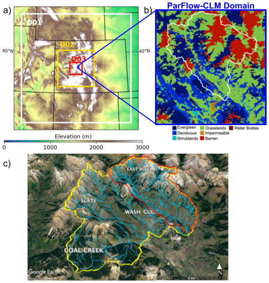
Figure 1(a) Three nested WRF domains D01 (4.5 km grid resolution, 201 by 201 grid cells or 900 by 900 km extent), D02 (1.5 km grid resolution, 201 by 201 grid cells or 300 by 300 km extent), and D03 (0.5 km grid resolution, 201 by 201 grid cells or 100 by 100 km extent) and their associated elevations (left). The Global Multi-resolution Terrain Elevation Data 2010 (GMTED2010) elevation data in meters above mean sea-level is used in the WRF simulation. (b) The innermost ParFlow-CLM domain and spatial extent of the East River watershed (white line) and associated land cover type derived from the National Land Cover Dataset (NLCD) (Homer et al., 2020) and upscaled to 100 m (right). (c) Topography and stream network in the ERW and other nearby watersheds.
A major experimental design decision when simulating the integrated mountainous hydrologic cycle is the computational cost associated with the simulations (e.g., simulated years per actual day) that are determined by model horizontal, vertical, and time step resolutions as well as subgrid-scale physics parameterization complexity. The computational expense incurred here to explore the sensitivities of WRF configuration choices was significant: 1 simulated year requires approximately 100 000 CPU hours on Lawrence Berkeley National Laboratory's Lawrencium lr6 supercomputing system. As such, it was highly impractical to simulate the entire configuration space of meteorological forcing and subgrid-scale parameterization choice. A discrete subsample of configurations, as presented here, is used to isolate and systematically determine which combination of subgrid-scale parameterization choice is superior for a given domain such as the ERW. We therefore adopted a parsimonious approach to explore the space of possible WRF configurations, described below.
3.1.1 Subgrid-scale physics schemes
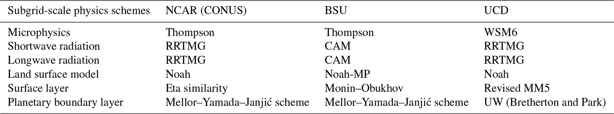
Three well-established suites of subgrid-scale physics schemes for WRF are evaluated in this study (Table 1). One scheme was developed by NCAR and is used for a wide range of simulations over domains extending across the entire conterminous United States (CONUS) (Liu et al., 2017). Another scheme that we consider here has been used for decadal-length hydroclimate simulation over California (Huang et al., 2016; Xu et al., 2018; Ullrich et al., 2018), and since it was initially developed by researchers at the University of California, Davis, it is denoted as UCD here. More recently, Rudisill et al. (2021) implemented a WRF configuration that focused on exploring land–atmosphere interactions in complex terrain. This configuration was developed by researchers at Boise State University and is referred to as BSU here. We recognized that this study would be computationally constrained given our prioritization of the use of sub-kilometer horizontal resolution IPM simulations, and this is why we did not exhaustively sample the model configuration matrix.
Table 1Microphysics, radiation, land surface model, surface layer, and planetary boundary layer schemes used for the three different WRF configurations of the IPM tested here.
3.1.2 Meteorological forcing
Each of these WRF configurations must specify a set of initial and lateral boundary conditions at the synoptic scale and, at least in the outer domain, are typically derived from high-resolution atmospheric reanalyses. The reanalysis from the National Centers for Environmental Prediction (NCEP), the Climate Forecast System Reanalysis version 2 (CFSR2), the Modern-Era Retrospective analysis for Research and Applications – Version 2 (MERRA2), and the European Centre for Medium-Range Weather Forecasting Reanalysis version 5 (ERA5) were used in this study.
ERA5 is the fifth-generation ECMWF atmospheric reanalysis of the global climate on a 30 km grid resolution (Hersbach et al., 2020), and combines model data with observations from across the world into a globally complete and consistent dataset. The CFSR2 is also global and is designed to provide an operational product for forecasting and analysis purposes at 0.3∘ grid resolution (Saha et al., 2010). The CFSR2 data were generated by an advanced assimilation scheme, which assimilates satellite radiation using an atmosphere–land–sea ice coupling approach. MERRA2 is another atmospheric reanalysis based on data assimilation (Gelaro et al., 2017), which is the first long-term global reanalysis to assimilate space-based observations of aerosols and represent their interactions with other physical processes in the climate system. In addition, the NCEP FNL (National Centers for Environmental Prediction, 2000) operational global analysis and forecast data are on a 0.25∘ grid resolution from the Global Data Assimilation System (GDAS) (Kleist et al., 2009). All meteorological forcing datasets are processed at a 6-hourly resolution by the WRF Preprocessing System (WPS).
3.1.3 Topographic radiation
Topographic effects for shortwave radiation flux calculations in complex terrain are evaluated (Arthur et al., 2018). One is the “slope_rad” namelist option, which modifies surface solar radiation flux according to terrain slope by correcting it based on the solar zenith angle relative to the local surface normal vector. This adjustment ensures that the solar radiation received at the surface in WRF is consistent with the geometric projection of incoming sunlight onto local, non-flat surfaces. The other namelist option, “topo_shading”, allows for shadowing of neighboring grid cells. When topo_shading is active, WRF determines if any topography intersects a line drawn between a given grid point and the location of the sun at the time step of the WRF run. If so, a topographic shadow is cast on that grid point, and the direct component of the incoming solar radiation is set to 0. In this study, simulations in which slope_rad and topo_shading are jointly enabled are termed “3DRad”, and when they are jointly disabled they are termed “no3DRad”, in the inner domain of the WRF simulation.

Figure 2Conceptual framework for developing a set of different WRF configurations of the IPM to evaluate the sensitivities of subgrid-scale physics parameterization choice, meteorological forcing, and radiation scheme in the representation of mountain water and energy budgets.
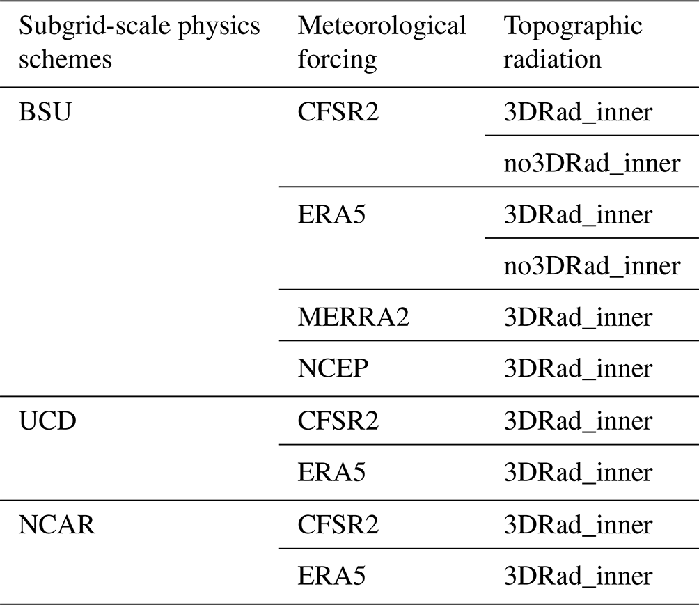
Table 2East River watershed WRF experiment configurations. Three subgrid-scale physics schemes, four meteorological forcings, and the topographic radiation options were assessed.
3.2 ParFlow-CLM description
ParFlow is a physically based surface–subsurface hydrologic model that solves the coupled flow of saturated and variability-saturated groundwater and overland surface water (Ashby and Falgout, 1996; Jones and Woodward, 2001; Maxwell, 2013). The three-dimensional form of Richards' equation is used to solve for lateral and vertical groundwater flow in the subsurface, and the kinematic wave approximation is used to solve two-dimensional overland flow. ParFlow is coupled to the land surface model, the Common Land Model (CLM), which calculates a coupled water energy balance at every surface cell of the domain (Dai et al., 2003) and incorporates spatially distributed vegetative processes by including specified land use types parameterized by the International Geosphere-Biosphere Program standard database. Hourly meteorological forcing derived from WRF drives ParFlow-CLM and includes the following eight variables: precipitation, 2 m surface air temperature, longwave radiation, shortwave radiation, 10 m east–west and south–north wind speeds, atmospheric pressure, and specific humidity. We also forced ParFlow-CLM with PRISM precipitation and temperature fields by evenly distributing daily precipitation and temperature across a diurnal cycle of 24 h within a day.
The ParFlow-CLM subsurface domain is 30 m deep at 100 m horizontal resolution. The WRF outputs are re-gridded using bilinear interpolation to match the ParFlow-CLM grid cells. The model parameters are based on a variety of geological and soil parameters and calibrated using streamflow measurements. More details can be found in Foster and Maxwell (2019) and Pribulick et al. (2016). The computational expense of ParFlow-CLM is also less substantial than that of WRF for this model configuration but still requires high-performance computing. Excluding the time for a multi-year initial condition spinup, a single water year of the ParFlow-CLM simulations on 64 cores on the NERSC's Cori supercomputing system is approximately 1000 CPU hours.
3.3 Reference datasets
The Parameter-elevation Relationships on Independent Slopes Model (PRISM) dataset (Daly et al., 2008) was used here as a point of comparison in evaluating model uncertainty across subgrid-scale physical schemes and meteorological forcing datasets for precipitation and temperature. PRISM uses observations from quality-controlled meteorological stations along with a topographic correction method against elevation based on empirical regressions to create daily gridded 800 m total precipitation and daily average, minimum and maximum 2 m surface temperature. Although PRISM was generated using statistical models, it has been widely used for climate and hydrological model assessments (e.g., Lundquist et al., 2019) and associated uncertainty analyses (e.g., Buban et al., 2020). In the assessment of subgrid-scale physics schemes and meteorological conditions, the percent difference in cumulative precipitation is compared against PRISM by calculating by (max − min) min ⋅ 100, where max and min are the maximum and minimum cumulative precipitation values from the simulations within each group, respectively.
Snowpack Telemetry (SNOTEL) data have been widely used in snowpack assessment (Serreze et al., 1999; Fassnacht et al., 2003), and we use three SNOTEL stations (Butte, Schofield Pass, Upper Taylor) within the WRF inner domain to assess the snowpack simulation skill of each IPM configuration. Significant heterogeneity is sampled by the three SNOTEL stations (within or near the ERW) due to the complex topography. For example, the Butte station is located downstream of the ERW and, on average, receives approximately 0.8 m of precipitation and reaches 0.4 m in maximum snow water equivalent over the year. On the other hand, the Schofield Pass station is located upstream of the ERW and, on average, receives 1.2 m of precipitation and reaches 0.9 m in maximum snow water equivalent. In addition, we use the snow water equivalent product of the Airborne Snow Observatory (ASO; Painter et al., 2016) on 7 April 2019 to evaluate the spatial pattern skill of the snowpack simulation across WRF configurations (Fig. S8 in the Supplement). The raw ASO product has 50 m spatial resolution and is regridded to the same grid resolution as WRF outputs (500 m) for comparison purposes using bilinear interpolation, as documented in Oaida et al. (2019). Since the spatial resolution of ASO data is significantly finer than the WRF outputs, we acknowledge that the underestimation by ASO could be due to the point-to-grid errors (Oaida et al., 2019). Notably, ASO SWE estimates are lower than SNOTEL SWE measurements (ASO: 389 mm at Butte, 938 mm at Schofield Pass; SNOTEL: 490 mm at Butte, 1260 mm at Schofield Pass). In addition to SNOTEL station data, stream gauge measurement of discharge at the pump house, the outlet of the ERW, is used to evaluate the ParFlow-CLM simulation results.
4.1 Subgrid-scale physical schemes vs. meteorological forcings
We start by presenting a number of time series of spatial averages over the ERW for WY19. They indicate the gross performance of the IPM across the water year and whether a configuration produces generally reasonable estimates relative to observational products. Figure 3 shows cumulative precipitation, 2 m surface air temperature, and snow water equivalent (SWE) aggregated over the ERW, and the in situ assessments compared against two SNOTEL stations are in Fig. S3. For cumulative precipitation, each configuration produces amounts higher than PRISM (cumulative precipitation of 1201 mm), and the UCD simulates the highest cumulative precipitation. For surface air temperature, the seasonal cycle and daily variability are captured by all configurations; however they exhibit systematic cold biases relative to PRISM (annual average 2 m surface air temperature of 0.6 ∘C). In terms of SWE, all model configurations concur in their representation of the snowpack accumulation season and melt season in late spring and into summer, except UCD, which simulates an earlier peak timing of SWE.
The spread in cumulative precipitation when comparing across different meteorological forcing datasets is apparent (Fig. 3). Although UCD and NCAR configurations show a greater difference in precipitation forced by ERA5 and CFSR2, the consistency across BSU configurations is notable, which also shows the closest agreement with PRISM. When comparing the relative roles of subgrid-scale physics scheme choices to meteorological forcings, the percent difference of cumulative precipitation, calculated by (maximum − minimum) minimum ⋅ 100, across BSU-CSFR2, UCD-CSFR2, and NCAR-CSFR2 schemes is nearly 34 % of the minimum cumulative precipitation simulated by BSU-CFSR2, compared to the 4.6 % of the simulations across BSU configurations with different meteorological forcing (CSFR2, ERA5, MERRA2, and NCEP).
BSU simulations are generally in agreement with PRISM. However, the UCD simulations are outliers relative to the other simulations, with cumulative precipitation of 1706 mm, or 42 % higher at the end of the water year, with the most notable differences occurring in March through September. NCAR simulations show general agreement with PRISM and BSU throughout the water year, save for June through September. The 2 m surface air temperature time series reveals that the UCD simulation is systematically colder throughout the winter and spring, regardless of which meteorological forcing dataset is used. The persistent cold bias simulated by the UCD, NCAR, and BSU schemes has been found in previous WRF studies within western US mountain regions (Xu et al., 2018; Rudisill et al., 2021). The SWE time series again shows a similar relationship with precipitation, with the outlier being UCD-ERA5, in terms of the seasonal timing of when snowpack peaks and melts (Fig. S1). Comparing the monthly average between UCD-ERA5 (Fig. S4) and BSU-ERA5 (Fig. S5), the early snowmelt observed in the UCD scheme is likely a result of warmer temperatures in the low-altitude region that melt the snow earlier in the water year. However, the high-altitude regions remain cold enough to maintain snowpack through early summer to midsummer.
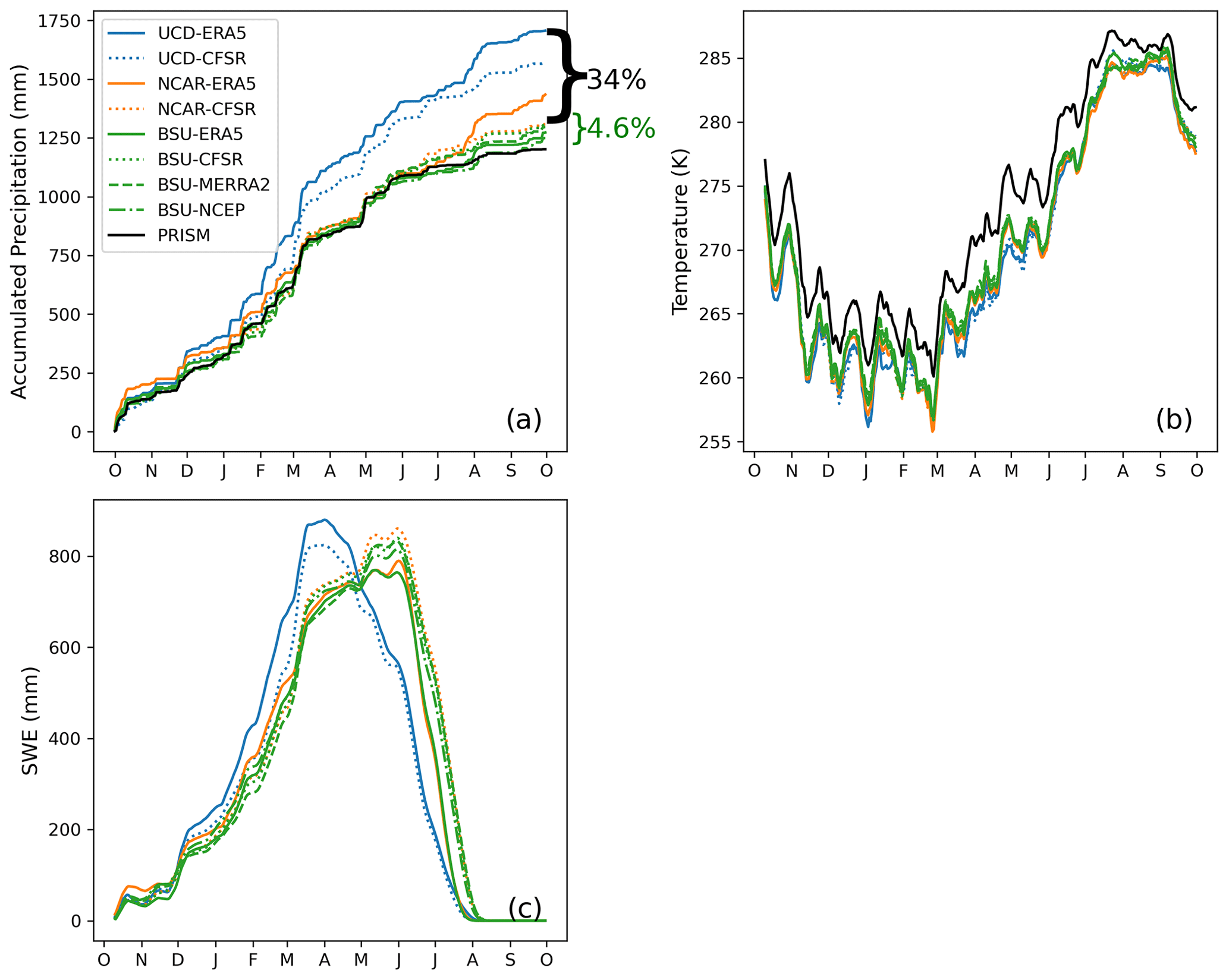
Figure 3(a) Cumulative precipitation, (b) 2 m surface air temperature, and (c) snow water equivalent (SWE) simulated within the ERW using an IPM with different subgrid-scale physics schemes and meteorological forcings. The cumulative precipitation and temperature results are compared relative to PRISM. The 10 d moving averages of daily temperature are shown in (b). The percent difference in cumulative precipitation across subgrid-scale physics schemes (black brackets) and meteorological forcing (green brackets), calculated by (maximum − minimum) minimum ⋅ 100, is provided on the right y axis.
In addition to the domain averages, spatial heterogeneity due to land surface cover and topographic effects is shown in Fig. 4. The systematic cold bias simulated throughout the water year appears to be an elevation-dependent phenomenon, with higher elevations exhibiting an enhanced cold bias compared with PRISM. However, the river valley and relatively lower-elevation areas at the southern edge of the ERW, which includes Crested Butte Mountain, stand out as these regions are warmer than the PRISM dataset. Figure 4b shows precipitation in BSU-CFSR2 is wetter in the western regions and drier in the eastern regions of the ERW in comparison to PRISM. Figure S3 shows comparisons between PRISM and the IPM configurations and indicates no biases that are persistent across seasons. During summer, the BSU-CFSR2 simulation consistently produces more precipitation than PRISM.
Although the 2 m surface air temperature bias is evident, it does not vary significantly across either subgrid-scale physics scheme or meteorological forcing. Therefore, subsequent exploration in this study will be focused on precipitation. The bottom row in Fig. 4 shows the grid-cell standard deviation of monthly precipitation across subgrid-scale physics schemes (i.e., UCD, NCAR and BSU simulations with CFSR2 meteorological forcing – bottom left) and BSU simulation driven by different meteorological forcing datasets (ERA5, CFSR2, MERRA2, and NCEP – bottom right). Similar to the conclusions drawn from Fig. 3, Fig. S6 also shows that the monthly spatial standard deviations across subgrid-scale physics schemes are generally greater than meteorological forcing, particularly in regions of higher elevation during the winter season.
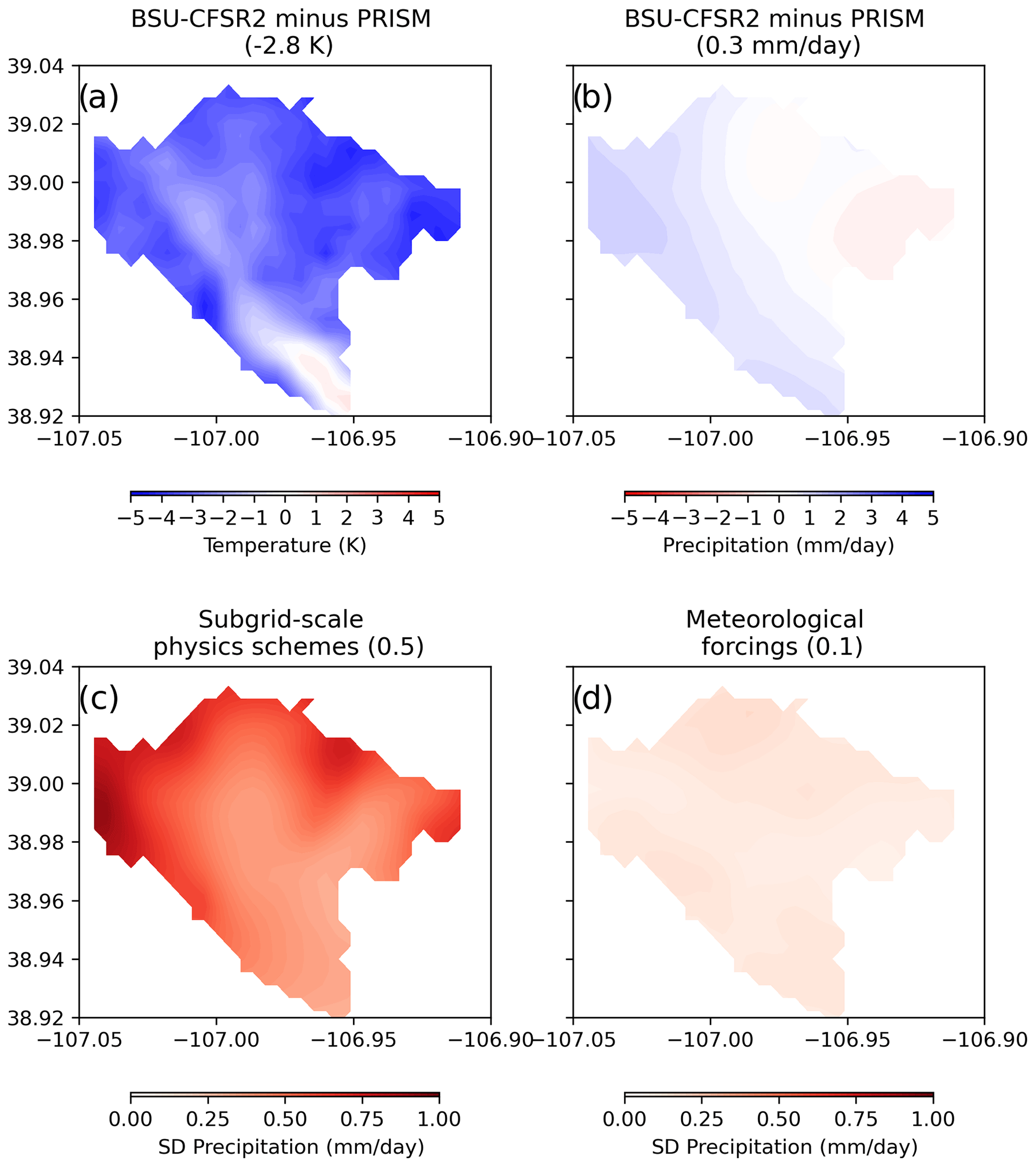
Figure 4Upper row: differences in spatial distributions of annual average 2 m surface air temperature (a) and cumulative precipitation (b) between the BSU-CFSR2 WRF configuration and PRISM. Lower row: for all schemes, the standard deviation of annual cumulative precipitation is plotted for subgrid-scale physics schemes (c) and meteorological forcings (d). The values in the parentheses are the domain-average differences over the water year. The standard deviations are the total annual precipitation in each ensemble simulations using different subgrid-scale physics schemes or large-scale meteorological forcings.
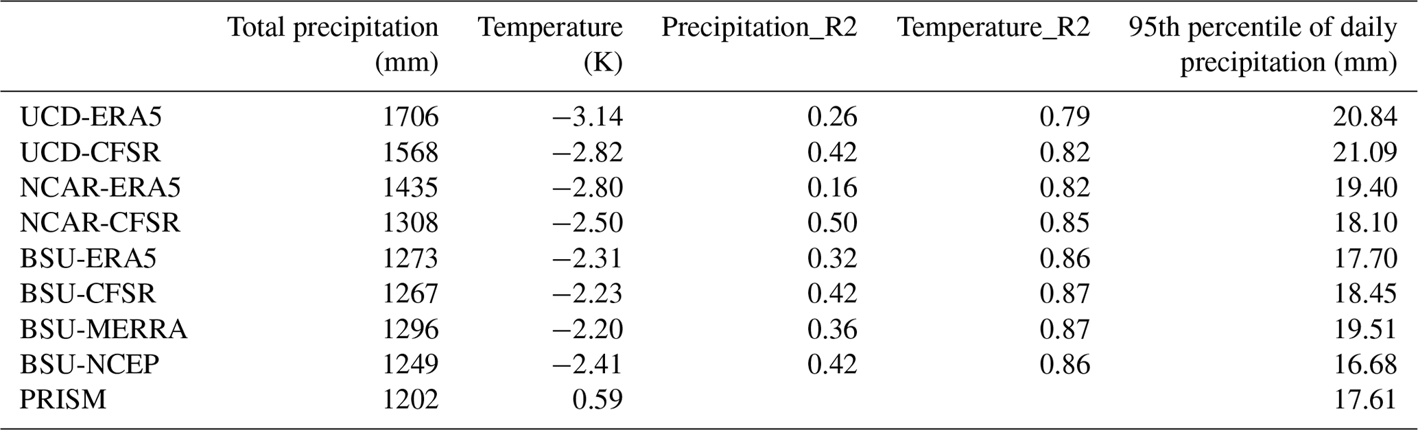
Quantitative statistics of the aggregated domain-average precipitation and temperature simulations for the WRF simulation across subgrid-scale physical schemes and large-scale meteorological forcings are presented in Table 3. Although NCAR-CFSR has a higher R2 than other simulations, NCAR-ERA5 has a very low R2. The BSU simulations provide a closer approximation of cumulative precipitation to PRISM. Specifically, BSU does better in simulating extreme precipitation events (i.e., 95th percentile). Therefore, we conclude that BSU WRF subgrid-scale physics schemes outperform the UCD and NCAR WRF subgrid-scale physics schemes in simulating both precipitation and temperature. On the other hand, the differences in precipitation and 2 m surface air temperatures across the four meteorological forcings are not statistically significant, and their standard deviations are much smaller than the differences in simulations across subgrid-scale physical schemes. While there are many metrics of model skill when selecting a meteorological forcing to simulate the hydrological processes in the ERW, we choose BSU-CFSR for the topographic radiation study in the next subsection due to its better match with PRISM, using our skill measures, in simulating both precipitation and 2 m surface air temperature.
Table 3Quantitative measures of precipitation and temperature of the WRF simulations among subgrid-scale physical schemes and meteorological forcings. R2 is the coefficient of determination for simulations and PRISM daily time series.
4.2 3D topographic radiation effects
Based on the assessment of simulated precipitation and 2 m surface air temperature compared with PRISM, the BSU-CFSR2 configuration is selected as a baseline to further explore the influence of topographic radiation scheme effects. The difference caused by turning on and off the 3D topographic radiation effects is similar in other WRF configurations; therefore, only the BSU-CFSR is presented. Figure 5 shows daily ERW spatial average time series over the water year for the major mountainous water and energy budget variables. By isolating the impacts of subgrid-scale physics schemes and meteorological forcings across IPM simulations, it is easier to systematically intercompare cause and effect across different topographic radiation options. Consistent with previous findings, all configurations still overestimate cumulative precipitation and are too cold relative to PRISM.

Figure 5Spatial-average cumulative precipitation, 2 m surface air temperature, and snow water equivalent (SWE) (first row) and shortwave and longwave radiation and latent and sensible heat (second row) over the ERW as simulated by the IPM configurations with and without realistic topographic radiation effects, along with, where available, estimates from PRISM. 3DRad indicates a simulation with topo_shading and slope_rad turned on in the WRF inner domain but not the outer WRF domains, and no3DRad indicates a simulation with top_shading and slope_rad turned off in both the inner and outer WRF domains. The 10 d moving averages are shown in (b) temperature and radiation variables (d, e, f, g).
Figure 6 shows the seasonally resolved shortwave radiation, 2 m surface air temperature, latent heat flux, and SWE for different configurations of shortwave radiation in the simulation with and without topo_shading and slope_rad options in the inner domain. While no3DRad does not adjust the SWdown (incoming shortwave radiation), the 3DRad simulation recalculates the SWdown based on the shadows cast by nearby topography. Spatial differences in IPM-simulated shortwave radiation (Fig. 6b) are seen in the northeast and western portions of the ERW, when the topographic effect of shortwave radiation is included. As a result, a corresponding change in the spatial pattern of simulated 2 m surface air temperature and latent heat flux is seen, driven by the change in downwelling shortwave radiation with topographic shading (Fig. 6a and d). Topographic shading makes a difference locally in latent heat (LH) flux, by redistributing the energy flux and thus affecting LH flux spatial distribution. Nevertheless, the domain-average LH flux remains unchanged between cases. The resulting pattern change in SWE (Fig. 6c) shows that the northern and northeastern sections of the ERW, where snowpack is concentrated, are sensitive to shortwave radiation. This is expected and consistent with previous findings that included topographic effects in shortwave radiation and found distinct spatial patterns of hydrologic variable sensitivity due to both shadows and surface reflection that produce time-varying effects on net surface radiation (Lee et al., 2015; Palazzi et al., 2019; Gu et al., 2020; Hao et al., 2021).
Although Fig. 5 shows that realistic shortwave radiation produces small effects on the seasonal cycle of the surface energy and mass budgets when averaged over the entire watershed, including annual average SWE (Fig. 5c), Fig. 6c shows that mountains and valleys have different amounts of SWE. Furthermore, seasonal patterns show simulated latent heat is diminished at lower elevations from March to May, when snowmelt occurs in the valley, and the remaining snowpack in the mountains and late snowmelt in the 3DRad simulation cause the lower latent heat flux shown in July (Fig. S7). The 3D radiation shading scheme does not significantly affect the total water balance but rather the spatial distribution of radiation fluxes. Thus, despite having minimal impacts on water impacting on the water balance, the scheme does have important localized impacts on SWE and surface energy budget spatial patterns. The 3DRad simulation has less SWE in the valleys during the accumulation season but more SWE at higher elevations during the melt season, which is a direct result of the differences in shortwave radiation redistribution. Figure S5 also shows that the latent heat differences in north-facing and south-facing sides are most apparent in the snowmelt and warm seasons. This is consistent with previous findings (Lee et al., 2015; Palazzi et al., 2019; Gu et al., 2020; Hao et al., 2021), that a more realistic treatment of shortwave radiation, which includes shadows and projected insolation on sloped surfaces, results in lower shortwave insolation on the surface at this time of year. The lower shortwave radiation should, in turn, decrease the energy available for the IPM to produce snowmelt. In summary, the simulations show that, while local spatial differences in surface radiation with and without realistic topography are apparent in Fig. 6, the domain spatial averages (even for SWE) are the same between shaded and non-shaded formulations. This suggests that while localized differences may be highlighted when shading is included, the impact of topographic shading on the entire water balance over a spatial domain like the ERW is negligible.

Figure 6Topographic radiation differences (3dRad minus no3dRad) annual average 2 m surface air temperature, shortwave (SW) and latent heat flux, and snow water equivalent (SWE) over the ERW. The values in the parentheses are the ERW average differences over the water year, which are small and consistent with Fig. 5.
4.3 Hydrological and streamflow responses
We have evaluated the aforementioned WRF configurations' subgrid-scale physical scheme and large-scale meteorological forcings in representing precipitation, temperature, snowpack, and radiation fluxes and their impacts on the integrated water budget within the ParFlow-CLM. We also evaluated the simulated discharge from ParFlow-CLM forced by PRISM as a comparison with WRF forcings. Figure 7 shows the simulated hydrologic output from the ParFlow-CLM model for watershed outlet discharge (top row) and watershed-average groundwater storage (bottom row). Discharge at the watershed outlet (see exact location in Fig. 1) shows a different timing across the various WRF subgrid-scale physics scheme configurations and large-scale meteorological forcings that lead to a temporal shift in simulated streamflow, where the daily averaged time series (left) shows only minor differences through time. However, cumulative discharge by the year-end reveals substantial differences (right), especially after peak snowmelt where estimates of cumulative discharge begin to diverge. Differences across the WRF configurations are especially large; the difference across the three subgrid-scale physics scheme configurations with ERA5 (UCD, NCAR, and BSU) varies by 26 % by the year-end. Differences across meteorological forcing (using the BSU physics configuration as a control, shown in green) are also noteworthy, although smaller, approximately 6 %. These results are consistent with the variation of simulated precipitation in WRF described earlier, confirming that for this basin, meteorological forcing drives less variance on the hydrologic response than the subgrid-scale physics scheme configuration.
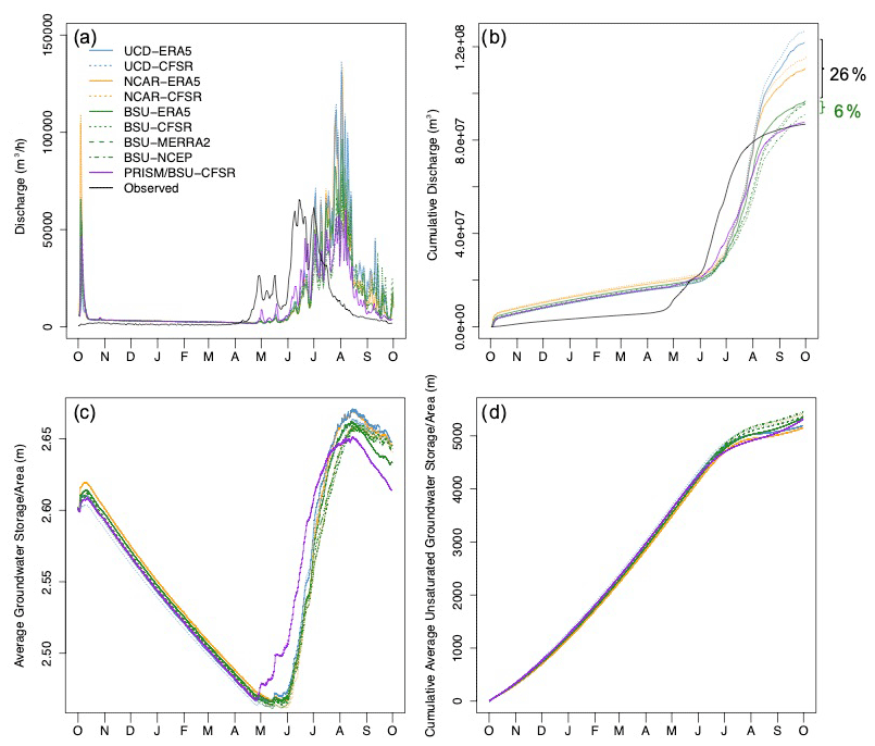
Figure 7Time series of ParFlow-CLM simulations of discharge rate (a), cumulative discharge (b), groundwater storage per unit area of the watershed (c), and cumulative average unsaturated groundwater storage per area of the watershed (d) for the IPM configurations described in Table 2. The brackets on the far right indicate the percent difference of cumulative discharge and unsaturated groundwater storage per area (b and d, respectively) for WRF simulations across different meteorological forcings (green) and subgrid-scale physics schemes (black).
In addition to the variance of cumulative discharge with WRF simulations across different conditions, a comparison to observed discharge is also shown in Fig. 7, which for all scenarios suggests a delayed snowmelt response in the IPM. While the objective of this study is not to replicate the observations, but rather determine sensitivity across IPM configuration choice, the mismatch in streamflow response suggests a systematic cold bias from the WRF input into ParFlow-CLM, which is consistent with the discussion surrounding Fig. 3 in relationship to PRISM. An early-fall peak in simulated discharge is also seen in all WRF simulations, and not in observed discharge, although a significant increase in SNOTEL precipitation was measured in October of that year (see Figs. S1, S2). This further supports a temperature bias, albeit opposite that of the cold bias discussed previously, where precipitation around that October storm event falling as rain (as opposed to snow) leads to a sharp increase in discharge. A sensitivity analysis of the BSU-ERA5 model run for a lower precipitation year (water year 2018, which was nearly half the precipitation of 2019) showed better agreement with observed discharge, which suggests the bias in timing may be a function of accumulated precipitation and/or snowmelt, and this is reserved for future studies (not shown).
Basin-average groundwater storage, shown in Fig. 7c in area-normalized units, shows a strong annual signal for all WRF configurations with minimal differences across IPM configurations. Here all groundwater, inclusive of saturated or unsaturated storage, is considered. The cumulative, area-normalized annual groundwater storage, when accounting for only vadose zone storage (Fig. 7d), which is most responsive to sub-annual differences in precipitation inputs, is meaningful in this context because it relates a cumulative impact on near-surface groundwater storage due to IPM configuration. Similar to the year-end cumulative discharge, year-end departures in vadose zone groundwater storage across the different simulations are evident. Differences across the IPM configurations of subgrid-scale physics schemes are larger than the difference across the forcing simulations (4 % versus 2 %, respectively). While the differences in groundwater signals are not as pronounced as the discharge signals, streamflow signals are very reactive and noisy and change quickly, whereas groundwater signals are the product of slower processes via infiltration and vadose zone dynamics, often at longer timescales, which result in very different temporal signals as compared to streamflow.
Figure 8 shows maps of standard deviations in annual total evapotranspiration (ET) simulated by ParFlow-CLM across IPM configurations (top row) and the cell-binned relationship of those standard deviations of annual ET with land use and cover type, as well as elevation (bottom). Consistent with variations shown in the simulated discharge and groundwater storage, ParFlow-CLM simulates greater variations of ET under WRF configurations driven by different subgrid-scale physics schemes (Fig. 8a), compared to the simulations conducted with different meteorological forcings (Fig. 8b). These results suggest that locations populated by high-water-demanding vegetation (namely evergreen and deciduous forests) at mid-elevations result in the highest ET variability across IPM configurations. Conversely, low-water-demanding vegetation (barren/sparsely vegetated land and grasses), which resides across a range of elevations in the study domain, results in the lowest variability in annual ET across IPM configurations. These differences in water demand essentially magnify any differences in atmospheric conditions.
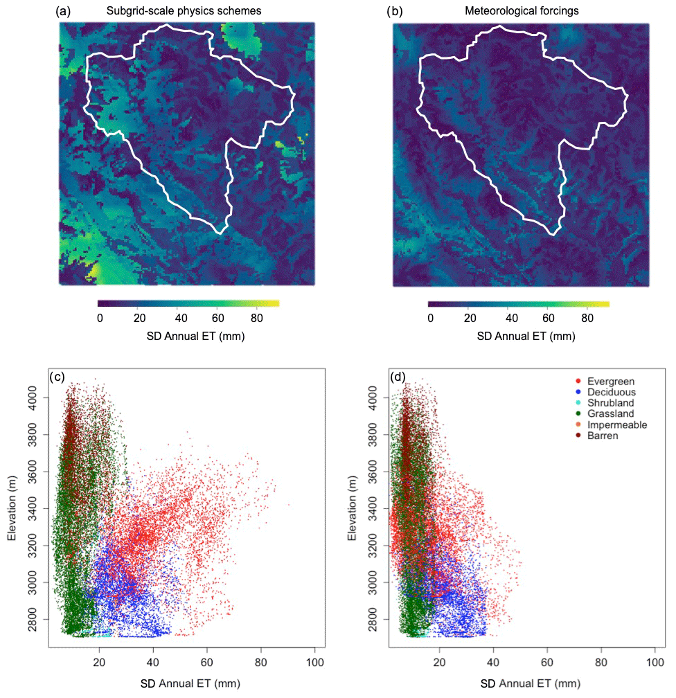
Figure 8Pixel-level standard deviation in annual total evapotranspiration (ET) over the ParFlow-CLM domain from WRF with different subgrid-scale physics schemes (a, c) or meteorological forcing (b, d). The ERW outline is overlaid in white in the upper row (a–b). The standard deviation of simulated ET from ParFlow-CLM across different physics schemes (c) and meteorological forcing (d) is presented in the lower row (c–d). For each pixel in (a)–(b), the relationship between annual ET standard deviation, elevation (y axis), and land cover type (colors) is shown by scatter plots on the bottom row (c–d). See Fig. 1 for maps of land cover types. Subgrid-scale physics schemes (a, c) have more variance compared to meteorological forcings (b, d), especially for mid-elevations and in evergreen forests.
5.1 Scientific findings
In spite of previous efforts to characterize the sensitivity of WRF simulations to model configuration choices, the mountain climate and hydrology scientific community has not sufficiently explored the implications of those choices for surface and subsurface hydrology in high-altitude complex terrain. Here, we used an IPM with one-way feedbacks from WRF to ParFlow-CLM to assess the hydrometeorology of the ERW, which is characterized by strong hydrological gradients indicative of mountain environments of the UCRB.
In this paper, we present a number of numerical experiment results that are informative for the scientific community to better understand atmosphere-through-bedrock process interactions and the uncertainties of those interactions between climate and hydrological model experimental setup choices. First, the uncertainties associated with meteorological forcing choice are less important than subgrid-scale physics scheme choice, at least in the ERW. This finding has important implications for IPM in complex terrain, since it reveals that the differences in reanalysis products are less consequential for initializing and forcing IPMs than atmospheric configurations and that efforts to advance IPMs such as collecting observations and using them to evaluate physical process parameterizations at the sub-HUC-8 (hydrologic unit code) scale could help to better constrain model performance. This result also shows that the large-scale meteorological forcing of the IPM simulation is less important in driving the magnitude and spatial variability of key hydrometeorological variables than the details in choosing and optimizing atmospheric subgrid-scale physics schemes (e.g., microphysics or boundary layer turbulence). Ultimately, we used the BSU-CFSR2 configuration to recreate WY2019 in the ERW, which allows researchers, in this case, to prioritize process studies and the development of associated observational constraints within the ERW. However, further investigation is needed to evaluate the systemic cold bias across IPM configurations, particularly at higher elevations, and the consequence of delayed snowmelt and timing of discharge peaks.
We recognize that numerous works in meteorological disciplines have demonstrated that “physical parameterization is much more important than lateral or initial conditions” (e.g., Solman and Pessacg, 2012; Pohl et al., 2011). However, our findings are not redundant with the published literature, as those references either evaluated large-scale meteorological processes or did not focus on high-altitude complex terrain regions, which are central to our study. Additionally, most IPM studies to date do not show how the range of reasonable IPM configurations (based on configurations that have been presented in the published literature) affects water-management-relevant processes such as discharge, ET, and subsurface hydrology. With our set of one-way atmosphere-through-bedrock process modeling results, we now show how choices in atmospheric process model configurations impact the surface and subsurface hydrology. Specifically, we evaluate and quantify the sensitivity of discharge, ET, and subsurface hydrology to IPM configurations, and we also address how 3D topographic radiation schemes affect both the spatial distribution and spatial average aspects of the mountainous hydrologic budget.
In the investigation of topographical and slope gradient effects on shortwave radiation, our study shows those considerations in WRF are essential in redistributing radiation flux over regions of complex terrain, even though the differences in spatial-average performance over ERW are minimal. This is because the spatial redistribution of shortwave radiation leads to approximately ±30 W m−2 difference in the east-/west-facing slopes that lead to ±1 K difference in 2 m surface air temperature in August and September (when snowpack is nonexistent). Throughout most of the water year when snowpack exists, the spatial heterogeneity of temperature differences is less apparent than for shortwave radiation. Latent heat buffers the differences of the shortwave radiation contribution to the radiation budget and causes early snowmelt in the high-elevation mountains in those simulations with topographical and slope gradient shortwave radiation effects turned on. At the same time, the systemic cold bias and limitations of one-way feedback in this study are potentially indicative of challenges in extrapolating findings from one mountainous watershed to another. If atmospheric process details are significant for surface and subsurface hydrological modeling, and if the findings regarding atmospheric processes in one study area are marginally or completely irrelevant to other mountainous watersheds, then additional fieldwork would be needed in mountainous hydrology research to address this issue, given that the extrapolation of fieldwork results remains a central challenge for field-based research and modeling activities.
5.2 Limitations and future works
A limitation of our study, given the computational constraints of running IPMs, is that it was infeasible to explore the full parameter spaces of WRF and ParFlow-CLM exhaustively; thus, our conclusions are limited to the selected subgrid-scale physics schemes and meteorological forcing datasets analyzed. Additional work is needed to improve the systemic cold bias in 2 m surface air temperature throughout all experiments as this may have been the major driver in the delayed snowmelt and peak discharge simulated by the IPM.
Another methodological constraint is that our WRF and ParFlow-CLM experiments were only one-way instead of two-way feedbacks, which ignores potentially important feedbacks from the subsurface hydrology to the atmosphere via ET and the radiation budget. For example, Givati et al. (2016) reported that simulated precipitation was improved with two-way coupling in WRF-Hydro compared to WRF-only, and Forrester et al. (2018) showed that boundary layer dynamics were impacted in IPM simulations in regions where shallow water tables exist. On the other hand, ParFlow-CLM is essential in our experiment for quantifying hydrological responses, including streamflow and groundwater storage. Although another fully coupled integrated hydrology model (i.e., WRF-Hydro) provides some insights into streamflow, it still uses a simplified and prescribed stream network. Groundwater storage in WRF-Hydro is also highly simplified, using a bucket model, while ParFlow-CLM simulates the full 3D continuum of variable saturation in three dimensions. Importantly, in a similar fashion to the hierarchy of climate models approach oft used in the climate community (Jeevanjee et al., 2017), we would also like to assess one-way coupling performance of our IPM prior to assessing two-way coupling IPM performance.
The East River watershed is already highly instrumented due to the presence of the long-standing Rocky Mountain Biological Laboratory (RMBL), the SNOTEL network, the United States Geological Survey's Next Generation Water Observing System (NGWOS), the National Science Foundation's Sublimation of Snow (SOS) project, and the DOE Watershed Science Focus Area project, which has been adding instrumentation to the watershed over the last ∼7 years. While these observations focus primarily on surface and subsurface processes, the East River watershed has become even more instrumented in recent years (2021–2023) through the support of the US DOE (SAIL campaign) and US NOAA (SPLASH campaign) deployments of a comprehensive set of atmospheric instrumentation (e.g., radar and radiation measurements). Future work will include integration of data, either indirectly through IPM benchmarking or directly through data assimilation into the IPM, from the SAIL campaign. SAIL is collecting a wide array of observations with the intent to advance understanding of precipitation, snow, aerosol, aerosol–cloud interaction, and radiation processes in complex terrain and establish the minimum but sufficient level of process understanding to develop a robust predictive understanding of seasonal surface water and energy budgets in the ERW (Feldman et al., 2021). SAIL aims to develop a wide range of hydrometeorological datasets to constrain atmosphere, surface, and subsurface processes simultaneously. Together, these resources are contributing to the establishment of a highly instrumented and in-depth-studied UCRB watershed. We look forward to building upon the knowledge learned from this paper to compare the most appropriately configured IPM to SAIL and SPLASH campaign observations. Our study highlights that the benchmarking provided by these data collections will be critical in addressing the systemic IPM cold bias by providing a more constrained estimate of radiation budgets in complex terrain that ultimately shape snowmelt and discharge.
All WRF model output files can be found at https://portal.nersc.gov/archive/home/z/zexuanxu/Shared/www/IPM (Xu et al., 2023).
Please notify corresponding author Zexuan Xu (zexuanxu@lbl.gov) if you have used our data.
The supplement related to this article is available online at: https://doi.org/10.5194/hess-27-1771-2023-supplement.
ZX, ERSW, AMR, and DF designed the study together. ZX performed the WRF simulations and analyzed the results. ERW performed the ParFlow-CLM simulations. All authors contributed to the writing and approved this paper.
The contact author has declared that none of the authors has any competing interests.
Publisher’s note: Copernicus Publications remains neutral with regard to jurisdictional claims in published maps and institutional affiliations.
This work was supported by the Laboratory Directed Research and Development Program of Lawrence Berkeley National Laboratory. This work was also supported by the Watershed Function Scientific Focus Area project, the Atmospheric System Research (ASR), and the Atmospheric Radiation Measurement (ARM) User Facility Program, funded by the U.S. Department of Energy, Office of Science, Office of Biological and Environmental Research, under U.S. Department of Energy contract no. DE-AC02-05CH11231. This research used resources of the National Energy Research Scientific Computing Center, a DOE Office of Science User Facility supported by the Office of Science of the U.S. Department of Energy under that same contract. This research also used the Lawrencium computational cluster resource provided by the IT Division at the Lawrence Berkeley National Laboratory (supported by the Director, Office of Science, Office of Basic Energy Sciences, of the U.S. Department of Energy under contract no. DE-AC02-05CH11231). The authors acknowledge the helpful guidance provided by Lejo Flores at Boise State University and Will Rudisill at Lawrence Berkeley National Laboratory regarding the WRF configurations conducted in this study over the ERW.
Authors Zexuan Xu, Erica R. Siirilla-Woodburn, and Daniel Feldman were supported by the Laboratory Directed Research and Development Program funded by Lawrence Berkeley National Laboratory, the Watershed Function Scientific Focus Area funded by the U.S. Department of Energy, Office of Science, Office of Biological and Environmental Research, and the Atmospheric Radiation Measurement User Facility Program of the U.S. Department of Energy, Office of Science, Office of Biological and Environmental Research, under U.S. Department of Energy contract no. DE-AC02-05CH11231. Co-author Alan M. Rhoades was funded by the Director, Office of Science, Office of Biological and Environmental Research of the U.S. Department of Energy Regional and Global Model Analysis (RGMA) program through the Calibrated and Systematic Characterization, Attribution and Detection of Extremes (CASCADE) Science Focus Area (award no. DE-AC02-05CH11231), and the “An Integrated Evaluation of the Simulated Hydroclimate System of the Continental US” project (award no. DE-SC0016605).
This paper was edited by Xing Yuan and reviewed by three anonymous referees.
Alder, J. R. and Hostetler, S. W.: The dependence of hydroclimate projections in snow-dominated regions of the western United States on the choice of statistically downscaled climate data, Water Resour. Res., 55, 2279–2300, 2019.
Arthur, R. S., Lundquist, K. A., Mirocha, J. D., and Chow, F. K.: Topographic effects on radiation in the WRF Model with the immersed boundary method: Implementation, validation, and application to complex terrain, Mon. Weather Rev., 146, 3277–3292, https://doi.org/10.1175/MWR-D-18-0108.1, 2018.
Ashby, S. F. and Falgout, R. D.: A parallel multigrid preconditioned conjugate gradient algorithm for groundwater flow simulations, Nucl. Sci. Eng., 124, 145–159, https://doi.org/10.13182/NSE96-A24230, 1996.
Buban, M. S., Lee, T. R., and Baker, C. B.: A comparison of the US climate reference network precipitation data to the parameter-elevation regressions on independent slopes model (PRISM), J. Hydrometeorol., 21, 2391–2400, 2020.
Camera, C., Bruggeman, A., Zittis, G., Sofokleous, I., and Arnault, J.: Simulation of extreme rainfall and streamflow events in small Mediterranean watersheds with a one-way-coupled atmospheric–hydrologic modelling system, Nat. Hazards Earth Syst. Sci., 20, 2791–2810, https://doi.org/10.5194/nhess-20-2791-2020, 2020.
Comin, A. N., Schumacher, V., Justino, F., and Fernandez, A.: Impact of different microphysical parameterizations on extreme snowfall events in the Southern Andes, Weather Climate Extremes, 21, 65–75, https://doi.org/10.1016/j.wace.2018.07.001, 2018.
Dai, Y., Zeng, X., Dickinson, R. E., Baker, I., Bonan, G. B., Bosilovich, M. G., Denning, A. S., Dirmeyer, P. A., Houser, P. R., Niu, G., Oleson, K. W., Schlosser, C. A., and Yang, Z.: The Common Land Model, B. Am. Meteorol. Soc., 84, 1013–1024, https://doi.org/10.1175/BAMS-84-8-1013, 2003.
Davison, J. H., Hwang, H.-T., Sudicky, E. A., Mallia, D. V., and Lin, J. C.: Full coupling between the atmosphere, surface, and subsurface for integrated hydrologic simulation, J. Adv. Model. Earth Sy., 10, 43–53, 2018.
Daly, C., Halbleib, M., Smith, J. I., Gibson, W. P., Doggett, M. K., Taylor, G. H., Curtis, J., and Pasteris, P. P.: Physiographically sensitive mapping of climatological temperature and precipitation across the conterminous United States, Int. J. Climatol., 28, 2031–2064, https://doi.org/10.1002/joc.1688, 2008.
Fassnacht, S., Dressler, K., and Bales, R.: Snow water equivalent interpolation for the Colorado River Basin from snow telemetry (SNOTEL) data, Water Resour. Res., 39, 1208, https://doi.org/10.1029/2002WR001512, 2003.
Feldman, D., Aiken, A., Boos, W., Carroll, R., Chandrasekar, V., Collins, W., Collis, S., Deems, J., DeMott, P., Fan, J., and Flores, A.: Surface Atmosphere Integrated Field Laboratory (SAIL), Science Plan, edited by: Stafford, R., ARM user facility, DOE/SC-ARM-21-004, https://www.osti.gov/servlets/purl/1781024 (last access: 27 April 2023), 2021.
Forrester, M. M., Maxwell, R. M., Bearup, L. A., and Gochis, D. J.: Forest disturbance feedbacks from bedrock to atmosphere using coupled hydrometeorological simulations over the Rocky Mountain headwaters, J. Geophys. Res.-Atmos., 123, 9026–9046, https://doi.org/10.1029/2018JD028380, 2018.
Foster, M. and Maxwell, R.: Sensitivity analysis of hydraulic conductivity and Manning's n parameters lead to new method to scale effective hydraulic conductivity across model resolutions, Hydrol. Process., 33, 332–349, 2019.
Gelaro, R., McCarty, W., Suárez, M. J., Todling, R., Molod, A., Takacs, L., Randles, C. A., Darmenov, A., Bosilovich, M. G., Reichle, R., and Wargan, K.: The modern-era retrospective analysis for research and applications, version 2 (MERRA-2), J. Climate, 30, 5419–5454, https://doi.org/10.1175/JCLI-D-16-0758.1, 2017.
Givati, A., Gochis, D., Rummler, T., and Kunstmann, H.: Comparing one-way and two-way coupled hydrometeorological forecasting systems for flood forecasting in the Mediterranean region, Hydrology, 3, 19, https://doi.org/10.3390/hydrology3020019, 2016.
Gu, C., Huang, A., Wu, Y., Yang, B., Mu, X., Zhang, X., and Cai, S.: Effects of subgrid terrain radiative forcing on the ability of RegCM4. 1 in the simulation of summer precipitation over China, J. Geophys. Res.-Atmos., 125, e2019JD032215, https://doi.org/10.1029/2019JD032215, 2020.
Gutowski Jr., W. J., Ullrich, P. A., Hall, A., Leung, L. R., O'Brien, T. A., Patricola, C. M., Arritt, R. W., Bukovsky, M. S., Calvin, K. V., Feng, Z., Jones, A. D., Kooperman, G. J., Monier, E., Pritchard, M. S., Pryor, S. C., Qian, Y., Rhoades, A. M., Roberts, A. F., Sakaguchi, K., Urban, N., and Zarzycki, C.: The Ongoing Need for High-Resolution Regional Climate Models: Process Understanding and Stakeholder Information, B. Am. Meteorol. Soc., 101, E664–E683, https://doi.org/10.1175/BAMS-D-19-0113.1, 2020.
Hao, D., Bisht, G., Gu, Y., Lee, W.-L., Liou, K.-N., and Leung, L. R.: A parameterization of sub-grid topographical effects on solar radiation in the E3SM Land Model (version 1.0): implementation and evaluation over the Tibetan Plateau, Geosci. Model Dev., 14, 6273–6289, https://doi.org/10.5194/gmd-14-6273-2021, 2021.
Hersbach, H., Bell, B., Berrisford, P., Hirahara, S., Horányi, A., Muñoz‐Sabater, J., Nicolas, J., Peubey, C., Radu, R., Schepers, D., and Simmons, A.: The ERA5 global reanalysis, Q. J. Roy. Meteorol. Soc., 146, 1999–2049, https://doi.org/10.1002/qj.3803, 2020.
Homer, C., Dewitz, J., Jin, S., Xian, G., Costello, C., Danielson, P., Gass, L., Funk, M., Wickham, J., Stehman, S., and Auch, R.: Conterminous United States land cover change patterns 2001–2016 from the 2016 National Land Cover Database, ISPRS J. Photogramm., 162, 184–199, https://doi.org/10.1016/j.isprsjprs.2020.02.019, 2020.
Huang, X., Rhoades, A. M., Ullrich, P. A., and Zarzycki, C. M.: An evaluation of the variable-resolution CESM for modeling California's climate, J. Adv. Model. Earth Sy., 8, 345–369, https://doi.org/10.1002/2015MS000559, 2016.
Hubbard, S. S., Williams, K. H., Agarwal, D., Banfield, J., Beller, H., Bouskill, N., Brodie, E., Carroll, R., Dafflon, B., Dwivedi, D., and Falco, N.: The East River, Colorado, Watershed: A mountainous community testbed for improving predictive understanding of multiscale hydrological–biogeochemical dynamics, Vadose Zone J., 17, 1–25, https://doi.org/10.2136/vzj2018.03.0061, 2018.
James, T., Evans, A., Madly, E., and Kelly, C.: The economic importance of the Colorado River to the basin region, Final Rep., L. William Seidman Research Institute, Arizona State University, 54, https://businessforwater.org/wp-content/uploads/2016/12/PTF-Final-121814.pdf (last access: 20 April 2023), 2014.
Jeevanjee, N., Hassanzadeh, P., Hill, S., and Sheshadri, A.: A perspective on climate model hierarchies, J. Adv. Model. Earth Sy., 9, 1760–1771, 2017.
Jin, J., Miller, N. L., and Schlegel, N.: Sensitivity study of four land surface schemes in the WRF model, Adv. Meteorol., 2010, 167436, https://doi.org/10.1155/2010/167436, 2010.
Jones, J. E. and Woodward, C. S.: Newton–Krylov-multigrid solvers for large-scale, highly heterogeneous, variably saturated flow problems, Adv. Water Resour., 24, 763–774, https://doi.org/10.1016/S0309-1708(00)00075-0, 2001.
Kleist, D. T., Parrish, D. F., Derber, J. C., Treadon, R., Wu, W.-S., and Lord, S.: Introduction of the GSI into the NCEP global data assimilation system, Weather Forecast., 24, 1691–1705, https://doi.org/10.1175/2009WAF2222201.1, 2009.
Lee, W.-L., Gu, Y., Liou, K. N., Leung, L. R., and Hsu, H.-H.: A global model simulation for 3-D radiative transfer impact on surface hydrology over the Sierra Nevada and Rocky Mountains, Atmos. Chem. Phys., 15, 5405–5413, https://doi.org/10.5194/acp-15-5405-2015, 2015.
Liu, C., Ikeda, K., Thompson, G., Rasmussen, R., and Dudhia, J.: High-resolution simulations of wintertime precipitation in the Colorado Headwaters region: Sensitivity to physics parameterizations, Mon. Weather Rev., 139, 3533–3553, https://doi.org/10.1175/MWR-D-11-00009.1, 2011.
Liu, C., Ikeda, K., Rasmussen, R., Barlage, M., Newman, A. J., Prein, A. F., Chen, F., Chen, L., Clark, M., Dai, A., and Dudhia, J.: Continental-scale convection-permitting modeling of the current and future climate of North America, Clim. Dynam., 49, 71–95, https://doi.org/10.1007/s00382-016-3327-9, 2017.
Lundquist, J., Hughes, M., Gutmann, E., and Kapnick, S.: Our skill in modeling mountain rain and snow is bypassing the skill of our observational networks, B. Am. Meteorol. Soc., 100, 2473–2490, https://doi.org/10.1175/BAMS-D-19-0001.1, 2019.
Maina, F. Z., Siirila-Woodburn, E. R., and Vahmani, P.: Sensitivity of meteorological-forcing resolution on hydrologic variables, Hydrol. Earth Syst. Sci., 24, 3451–3474, https://doi.org/10.5194/hess-24-3451-2020, 2020.
Mallard, M. S., Spero, T. L., and Taylor, S. M.: Examining WRF's sensitivity to contemporary land-use datasets across the contiguous United States Using Dynamical Downscaling, J. Appl. Meteorol. Climatol., 57, 2561–2583, https://doi.org/10.1175/JAMC-D-17-0328.1, 2018.
Maxwell, R. M.: A terrain-following grid transform and preconditioner for parallel, large-scale, integrated hydrologic modeling, Adv. Water Resour., 53, 109–117, https://doi.org/10.1016/j.advwatres.2012.10.001, 2013.
Maxwell, R. M., Condon, L. E., and Kollet, S. J.: A high-resolution simulation of groundwater and surface water over most of the continental US with the integrated hydrologic model ParFlow v3, Geosci. Model Dev., 8, 923–937, https://doi.org/10.5194/gmd-8-923-2015, 2015.
Meixner, T., Manning, A. H., Stonestrom, D. A., Allen, D. M., Ajami, H., Blasch, K. W., Brookfield, A. E., Castro, C. L., Clark, J. F., Gochis, D. J., and Flint, A. L.: Implications of projected climate change for groundwater recharge in the western United States, J. Hydrol., 534, 124–138, 2016.
Milly, P. C. and Dunne, K. A.: Colorado River flow dwindles as warming-driven loss of reflective snow energizes evaporation, Science, 367, 1252–1255, https://doi.org/10.1126/science.aay9187, 2020.
National Centers for Environmental Prediction: NCEP FNL Operational Model Global Tropospheric Analyses, continuing from July 1999, Research Data Archive at the National Center for Atmospheric Research, Computational and Information Systems Laboratory, https://doi.org/10.5065/D6M043C6, 2000.
Oaida, C. M., Reager, J. T., Andreadis, K. M., David, C. H., Levoe, S. R., Painter, T. H., Bormann, K. J., Trangsrud, A. R., Girotto, M., and Famiglietti, J. S.: A high-resolution data assimilation framework for snow water equivalent estimation across the Western United States and validation with the airborne snow observatory, J. Hydrometeorol., 20, 357–378, 2019.
Orr, A., Listowski, C., Couttet, M., Collier, E., Immerzeel, W., Deb, P., and Bannister, D.: Sensitivity of simulated summer monsoonal precipitation in Langtang Valley, Himalaya, to cloud microphysics schemes in WRF, J. Geophys. Res.-Atmos., 122, 6298–6318, 2017.
Painter, T. H., Berisford, D. F., Boardman, J. W., Bormann, K. J., Deems, J. S., Gehrke, F., Hedrick, A., Joyce, M., Laidlaw, R., Marks, D., and Mattmann, C.: The Airborne Snow Observatory: Fusion of scanning lidar, imaging spectrometer, and physically-based modeling for mapping snow water equivalent and snow albedo, Remote Sens. Environ., 184, 139–152, https://doi.org/10.1016/j.rse.2016.06.018, 2016.
Palazzi, E., Mortarini, L., Terzago, S., and Von Hardenberg, J.: Elevation-dependent warming in global climate model simulations at high spatial resolution, Clim. Dynam., 52, 2685–2702, https://doi.org/10.1007/s00382-018-4287-z, 2019.
Pohl, B., Crétat, J., and Camberlin, P.: Testing WRF capability in simulating the atmospheric water cycle over Equatorial East Africa, Clim. Dynam., 37, 1357–1379, 2011.
Powers, J. G., Klemp, J. B., Skamarock, W. C., Davis, C. A., Dudhia, J., Gill, D. O., Coen, J. L., Gochis, D. J., Ahmadov, R., Peckham, S. E., and Grell, G. A.: The weather research and forecasting model: Overview, system efforts, and future directions, B. Am. Meteorol. Soc., 98, 1717–1737, https://doi.org/10.1175/BAMS-D-15-00308.1, 2017.
Pribulick, C. E., Foster, L. M., Bearup, L. A., Navarre‐Sitchler, A. K., Williams, K. H., Carroll, R. W. and Maxwell, R. M.: Contrasting the hydrologic response due to land cover and climate change in a mountain headwaters system, Ecohydrology, 9, 1431–1438, 2016.
Rahimi, S., Krantz, W., Lin, Y.-H., Bass, B., Goldenson, N., Hall, A., Lebo, Z. J., and Norris, J.: Evaluation of a Reanalysis-Driven Configuration of WRF4 Over the Western United States From 1980 to 2020, J. Geophys. Res.-Atmos., 127, e2021JD035699, https://doi.org/10.1029/2021JD035699, 2022.
Rasmussen, K. L., Prein, A. F., Rasmussen, R. M., Ikeda, K., and Liu, C.: Changes in the convective population and thermodynamic environments in convection-permitting regional climate simulations over the United States, Clim. Dynam., 55, 383–408, https://doi.org/10.1007/s00382-017-4000-7, 2020.
Rasmussen, R., Liu, C., Ikeda, K., Gochis, D., Yates, D., Chen, F., Tewari, M., Barlage, M., Dudhia, J., Yu, W., and Miller, K.: High-resolution coupled climate runoff simulations of seasonal snowfall over Colorado: A process study of current and warmer climate, J. Climate, 24, 3015–3048, https://doi.org/10.1175/2010JCLI3985.1, 2011.
Rasmussen, R., Ikeda, K., Liu, C., Gochis, D., Clark, M., Dai, A., Gutmann, E., Dudhia, J., Chen, F., Barlage, M., and Yates, D.: Climate change impacts on the water balance of the Colorado headwaters: high-resolution regional climate model simulations, J. Hydrometeorol., 15, 1091–1116, https://doi.org/10.1175/JHM-D-13-0118.1, 2014.
Rhoades, A. M., Ullrich, P. A., and Zarzycki, C. M.: Projecting 21st century snowpack trends in western USA mountains using variable-resolution CESM, Clim. Dynam., 50, 261–288, https://doi.org/10.1007/s00382-017-3606-0, 2018a.
Rhoades, A. M., Ullrich, P. A., Zarzycki, C. M., Johansen, H., Margulis, S. A., Morrison, H., Xu, Z., and Collins, W. D.: Sensitivity of mountain hydroclimate simulations in variable-resolution CESM to microphysics and horizontal resolution, J. Adv. Model. Earth Sy., 10, 1357–1380, https://doi.org/10.1029/2018MS001326, 2018b.
Rhoades, A. M., Jones, A. D., and Ullrich, P. A.: Assessing mountains as natural reservoirs with a multimetric framework, Earth's Future, 6, 1221–1241, https://doi.org/10.1002/2017EF000789, 2018c.
Rudisill, W., Flores, A., and McNamara, J.: The Impact of Initial Snow Conditions on the Numerical Weather Simulation of a Northern Rockies Atmospheric River, J. Hydrometeorol., 22, 155–167, 2021.
Skamarock, W. C., Klemp, J. B., Dudhia, J., Gill, D. O., Liu, Z., Berner, J., Wang, W., Powers, J. G., Duda, M. G., Barker, D. M., and Huang, X. Y.: A description of the advanced research WRF model version 4, National Center for Atmospheric Research: Boulder, CO, USA, 145, p. 145, https://doi.org/10.5065/1dfh-6p97, 2019.
Saha, S., Moorthi, S., Pan, H. L., Wu, X., Wang, J., Nadiga, S., Tripp, P., Kistler, R., Woollen, J., Behringer, D., and Liu, H.: The NCEP climate forecast system reanalysis, B. Am. Meteorol. Soc., 91, 1015–1058, https://doi.org/10.1175/2010BAMS3001.1, 2010.
Schreiner-McGraw, A. P. and Ajami, H.: Impact of uncertainty in precipitation forcing data sets on the hydrologic budget of an integrated hydrologic model in mountainous terrain, Water Resour. Res., 56, e2020WR027639, https://doi.org/10.1029/2020WR027639, 2020.
Serreze, M. C., Clark, M. P., Armstrong, R. L., McGinnis, D. A., and Pulwarty, R. S.: Characteristics of the western United States snowpack from snowpack telemetry (SNOTEL) data, Water Resour. Res., 35, 2145–2160, https://doi.org/10.1029/1999WR900090, 1999.
Siirila-Woodburn, E. R., Rhoades, A. M., Hatchett, B. J., Huning, L. S., Szinai, J., Tague, C., Nico, P. S., Feldman, D. R., Jones, A. D., Collins, W. D., and Kaatz, L.: A low-to-no snow future and its impacts on water resources in the western United States, Nat. Rev. Earth Environ., 2, 800–819, https://doi.org/10.1038/s43017-021-00219-y, 2021.
Solman, S. A. and Pessacg, N. L.: Evaluating uncertainties in regional climate simulations over South America at the seasonal scale, Clim. Dynam., 39, 59–76, 2012.
Sturm, M., Goldstein, M. A., and Parr, C.: Water and life from snow: A trillion dollar science question, Water Resour. Res., 53, 3534–3544, https://doi.org/10.1002/2017WR020840, 2017.
Ullrich, P., Xu, Z., Rhoades, A., Dettinger, M., Mount, J., Jones, A., and Vahmani, P.: California's drought of the future: A midcentury recreation of the exceptional conditions of 2012–2017, Earth's Future, 6, 1568–1587, https://doi.org/10.1029/2018EF001007, 2018.
Walser, A. and Schär, C.: Convection-resolving precipitation forecasting and its predictability in Alpine river catchments, J. Hydrol., 288, 57–73, https://doi.org/10.1016/j.jhydrol.2003.11.035, 2004.
Winstral, A. and Marks, D.: Long-term snow distribution observations in a mountain catchment: Assessing variability, time stability, and the representativeness of an index site, Water Resour. Res., 50, 293–305, 2014.
Williams, A. P., Cook, B. I., and Smerdon, J. E.: Rapid intensification of the emerging southwestern North American megadrought in 2020–2021, Nat. Clim. Change, 12, 232–234, https://doi.org/10.1038/s41558-022-01290-z, 2022.
Xu, Y., Jones, A., and Rhoades, A.: A quantitative method to decompose SWE differences between regional climate models and reanalysis datasets, Sci. Rep., 9, 16520, https://doi.org/10.1038/s41598-019-52880-5, 2019.
Xu, Z., Rhoades, A. M., Johansen, H., Ullrich, P. A., and Collins, W. D.: An intercomparison of GCM and RCM dynamical downscaling for characterizing the hydroclimatology of California and Nevada, J. Hydrometeorol., 19, 1485–1506, https://doi.org/10.1175/JHM-D-17-0181.1, 2018.
Xu, Z., Siirila-Woodburn, E. R., Rhoades, A. M., and Feldman D.: Sensitivities of subgrid-scale physics schemes, meteorological forcing, and topographic radiation in atmosphere-through-bedrock integrated process models: a case study in the Upper Colorada River basin, NERSC Science Gateway [data set], https://portal.nersc.gov/archive/home/z/zexuanxu/Shared/www/IPM, last access: 20 April 2023.
Zhuang, X., Hao, Z., Singh, V. P., Zhang, Y., Feng, S., Xu, Y., and Hao, F.: Drought propagation under global warming: Characteristics, approaches, processes, and controlling factors, Sci. Total Environ., 838, 156021, https://doi.org/10.1016/j.scitotenv.2022.156021, 2022.
Zhang, Y. Y., Shao, Q. X., Ye, A. Z., Xing, H. T., and Xia, J.: Integrated water system simulation by considering hydrological and biogeochemical processes: model development, with parameter sensitivity and autocalibration, Hydrol. Earth Syst. Sci., 20, 529–553, https://doi.org/10.5194/hess-20-529-2016, 2016.