Technical note: Extending the SWAT model to transport chemicals through tile and groundwater flow

The Soil and Water Assessment Tool (SWAT) is frequently used to simulate the transport of water-soluble chemicals in the environment such as pesticides and their metabolites originating from agricultural applications. However, the model does not simulate the transport of chemicals through subsurface tile drains and groundwater. This limitation is particularly significant in lowland regions and when simulating stable chemicals that can leach into and accumulate in groundwater. To fill this gap, the publicly available SWAT code was modified to complement the simulation of chemicals by adding transport capabilities through tile and groundwater flow. The extended model was tested in two agricultural catchments with a typically used pesticide and one of its metabolites. Results show that the transport of the pesticide is mainly governed by surface runoff and that shallow surface tile flow contributions can be significant. Metabolite concentrations in streamflow are, however, driven by a complex spatiotemporal interplay of all surface and subsurface transport components. This highlights the advantages of applying the modified code in catchment-scale environmental exposure studies and for developing best management practices or mitigation strategies. The new code is made available as an electronic supplement to this technical note.

1 Introduction

Pesticide modeling on the watershed scale has evolved to significantly support the understanding of pesticide origin and transport pathways. It is also the only approach to analyze “what-if” scenarios for assessing anthropogenic pesticide inputs (Arabi et al., 2008), best management practices (Zhang and Zhang, 2011), and mitigation strategies to reduce pesticide concentrations in the environment (Holvoet et al., 2007). Many models have been developed that are considered appropriate for watershed-scale simulation of pesticides (Quilbe et al., 2006), of which the Soil and Water Assessment Tool (SWAT) was selected as one of three that were most suitable. SWAT (Arnold et al., 1998), a semi-distributed model, is well known for a wide range of hydrologic and water quality applications in catchments encompassing very small to very large areas worldwide (Gassman et al., 2007, 2014). The use of the SWAT model in simulating pesticide transport at the catchment-scale has been reported in the literature since at least 2005. An overview of peer-reviewed publications is provided in Winchell et al. (2018), who list studies conducted in North America (e.g., Vazquez-Amabile et al., 2006), Europe (e.g., Fohrer et al., 2014), and Asia (e.g., Bannwarth et al., 2014).

The standard SWAT model routes nutrients through all flow components. However, it simulates pesticide contributions to streams from surface runoff and erosion, as well as lateral subsurface flow only, and does not account for transport through subsurface tile drains and groundwater flow to streams. This simplification was made as many pesticides are mobilized by surface runoff and erosion, decayed on foliage and in soil, or moved out of the soil profile via lateral flow before they are expected to contribute to tile and groundwater flow. However, those additional transport pathways are relevant when simulating more stable, soluble, and mobile pesticides or metabolites (or other stable and mobile constituents and tracers), when working in environments with a strong interaction between surface water and groundwater, in regions with shallow groundwater tables, and in areas where tile drains exist.

The model extension presented here fills this gap by considering pesticide transport through tiles and groundwater return flow to surface waterbodies in SWAT.

2 Software description

2.1 SWAT model structure

The structure of the SWAT model allows for the prediction of flow, sediment, nutrients, and pesticide fluxes at multiple scales and locations throughout a watershed. The SWAT model divides the catchment into multiple subbasins. Subbasin delineation is based on the size of the catchment and the density of the stream network. Subbasins are created when two streams merge and can manually be added to represent each point where model predictions are required. A subbasin is divided into multiple hydrologic response units (HRUs), which are representative of unique combinations of land use, soils, and slope within a subbasin. Each HRU is considered an independent land unit within SWAT, and each HRU can have different parameterizations and agronomic practices, including tile drains. Within the soil layers of an HRU, fluxes are distinguished into surface runoff, lateral flow, and tile flow (if tile drains are present) that contribute to streams. Additionally, evaporation and recharge to groundwater occur. In up to two groundwater aquifers, the incoming water is partitioned into capillary rise (re-entering the soil profile from the shallow groundwater layer), storage, percolation, or outflow to streams. The second aquifer can either be unconnected (fluxes are lost from the system) or connected (fluxes are routed back to the streams). All outgoing HRU fluxes enter the streams at the upstream end of the segment and are routed to the downstream end, during which in-stream processes such as attenuation, partitioning, and degradation take place. The timing of HRU-level fluxes entering an associated stream is a function of the subbasin time of concentration and does not vary across HRUs. The process of a parent chemical forming a metabolite is not implemented in the current SWAT version. Thus, the metabolite formation requires a separate calculation and implementation in the model using “pseudo” chemical applications. For further information on the calculation of fluxes and concentrations of constituents, the reader is referred to the SWAT theoretical documentation (Neitsch et al., 2011).

2.2 Description of the new subsurface transport functionality

SWAT's source code (publicly available at https://bitbucket.org/blacklandgrasslandmodels/swat_development, last access: 5 January 2023; this study is based on version 681) consists of around 300 individual Fortran subroutines in which the processes and the functional modeling workflow are implemented. This modular structure allows the implementation of new functionalities through adding new routines or the modification of single subroutines.

Figure 1 shows a schematic representation of the newly implemented SWAT pesticide routing scheme. The current version of the SWAT model prevents soluble pesticides from leaching out of the soil profile (which includes the root zone below the maximum soil depth). Chemicals are prevented to flow through tile drains or entering the groundwater. While the tile and groundwater flow along with several loadings (e.g., nutrients) are simulated, the pesticide load is not routed. Thus, subroutines simulating subsurface flow and transport processes were modified to enable pesticide flux together with the tile flow and groundwater flows. The tile drain pesticide routing calculations were implemented in the pesticide leaching routine (pestlch.f) and a newly introduced subroutine (pestgw.f) contains the algorithms to simulate pesticide transport via shallow and deep groundwater flows.

Figure 1 Flow chart of the newly implemented pesticide routing functionality.

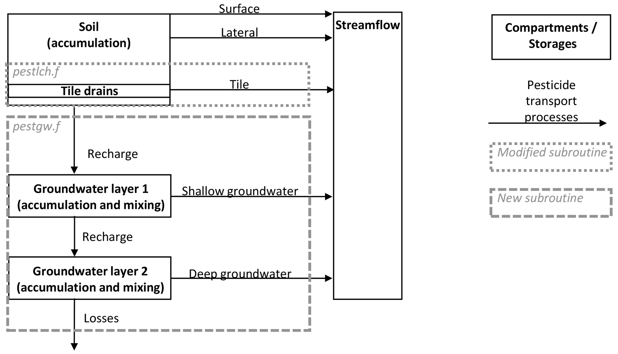
2.3 Tile drain flow pesticide implementation

Vertical and lateral pesticide movement within the soil layer as well as percolation out of the soil layer is calculated in subroutine pestlch.f. For adding the capability of routing pesticide through tile drains, corresponding equations were added to this subroutine. First, if tile drains are implemented in the respective soil layer, tile flow is added to the water that is leaving the layer (Eq. 1):

$$\begin{array}{}\text{(1)}& q_{\text{lyr}}=q_{\text{tile}}+q_{\text{prk}}+q_{\text{lat}},\end{array}$$

where q_lyr is the pesticide transport-effective flow leaving the tile-drained soil layer (without evaporation or plant uptake) (mm H₂O), q_tile is the tile flow leaving the soil layer (mm H₂O), q_prk is the percolation out of the layer (mm H₂O), and q_lat is the lateral flow leaving the soil layer (mm H₂O). Based on q_lyr, the amount of soluble pesticide leaving the tile-drained soil layer is calculated with Eq. (2) for each pesticide (see Neitsch et al., 2011, Chapter 4:3, and Leonard et al., 1987):

$$\begin{array}{}\text{(2)}& {\text{pst}}_{\text{rem}}={\text{sol}}_{\text{pst}}\cdot \left(\mathrm{1}-e^{-\frac{q_{\text{lyr}}}{w_{\text{sat}}+f_{\text{ads}}\cdot {\text{sol}}_{\text{bd}}\cdot {\text{sol}}_{\mathrm{d}}}}\right),\end{array}$$

where pst_rem is the total amount of soluble pesticide removed from the soil layer (kg ha⁻¹), sol_pst is the initial amount of total pesticide in the soil layer (kg ha⁻¹), w_sat is the amount of water in the soil layer at saturation (mm H₂O), f_ads is the soil adsorption coefficient ($\mathrm{mg}{\mathrm{kg}}^{-\mathrm{1}}/\mathrm{mg}{\mathrm{L}}^{-\mathrm{1}}$), sol_bd is the soil bulk density of the soil layer (mg m⁻³), and sol_d is the depth of the soil layer (mm). Pesticide concentration in tile flow is then calculated by dividing the amount of removed pesticide through the flow leaving the layer (Eq. 3):

$$\begin{array}{}\text{(3)}& {\text{pst}}_{\text{conc}}={\displaystyle \frac{{\text{pst}}_{\text{rem}}}{q_{\text{tile}}+q_{\text{prk}}+q_{\text{lat}}}},\end{array}$$

where pst_conc is the concentration of pesticide in the water (including the tile flow) leaving the soil layer ($\mathrm{kg}{\mathrm{ha}}^{-\mathrm{1}}{\mathrm{mm}}^{-\mathrm{1}}$). Finally, Eq. (4) is then as follows:

$$\begin{array}{}\text{(4)}& {\text{pst}}_{\text{tile}}={\text{pst}}_{\text{conc}}\cdot q_{\text{tile}},\end{array}$$

where pst_tile is the amount of pesticide leaving the soil layer through tile flow (kg ha⁻¹).

2.4 Groundwater flow pesticide implementation

The newly introduced subroutine pestgw.f contains equations to calculate pesticide transport via groundwater. First, the amount of pesticide in the shallow aquifer is calculated with Eq. (5):

$$\begin{array}{}\text{(5)}& \begin{array}{rl}{\text{pst}}_{\text{rchrg}}& =(\mathrm{1}-e^{-\mathrm{1.0}/{\text{gw}}_{\text{delay}}})\cdot {\text{pst}}_{\text{sol}}\\ & +e^{-\mathrm{1.0}/{\text{gw}}_{\text{delay}}}\cdot {\text{pst}}_{\text{rchrg–1}},\end{array}\end{array}$$

where pst_rchrg is the amount of pesticide entering the shallow aquifer (mg ha⁻¹), gw_delay is the time required for water and its soluble loadings to reach the shallow aquifer from the bottom of the root zone (d), pst_sol is the daily amount of pesticide leached from the soil profile (mg ha⁻¹), and pst_rchrg–1 is the amount of pesticide entering the shallow aquifer on the previous day (mg ha⁻¹). The current pesticide mass is tracked with Eq. (6):

$$\begin{array}{}\text{(6)}& {\text{pst}}_{\text{shallst}}={\text{pst}}_{\text{shallst–1}}+{\text{pst}}_{\text{rchrg}},\end{array}$$

where pst_shallst and pst_shallst–1 denote the amount of pesticide stored in the shallow aquifer on the present and previous day (kg ha⁻¹), respectively. Then, the pesticide groundwater contribution to streamflow is calculated as follows:

$$\begin{array}{}\text{(7)}& {\displaystyle }{\text{pst}}_{\text{shallconc}}={\displaystyle \frac{{\text{pst}}_{\text{shallst}}}{d_{\text{shall}}\cdot f_{\text{pstgw}}+q_{\text{gwshall}}+\text{revap}+q_{\text{gwseep}}}},\text{(8)}& {\displaystyle }{\text{pst}}_{\text{gwshall}}={\text{pst}}_{\text{shallconc}}\cdot q_{\text{gwshall}},\end{array}$$

where pst_shallconc is the pesticide concentration in shallow aquifer groundwater ($\mathrm{mg}{\mathrm{ha}}^{-\mathrm{1}}{\mathrm{mm}}^{-\mathrm{1}}$), d_shall is the depth of water in the shallow aquifer (mm H₂O), f_pstgw is the shallow groundwater pesticide mixing factor (dimensionless), q_gwshall is the shallow groundwater contribution to streamflow (mm H₂O), revap is the amount of water moving from the shallow aquifer into the soil profile or being taken up by plant roots in the shallow aquifer (mm H₂O), q_gwseep is the amount of water recharging the deep aquifer, and pst_gwshall is the amount of pesticide entering the channel via shallow aquifer groundwater flow (kg ha⁻¹). The amount of pesticide in the shallow aquifer is then updated as follows:

$$\begin{array}{}\text{(9)}& {\displaystyle }{\text{pst}}_{\text{gwseep}}={\text{pst}}_{\text{shallconc}}\cdot q_{\text{gwseep}},\text{(10)}& {\displaystyle }{\text{pst}}_{\text{shallst}}={\text{pst}}_{\text{shallst–1}}-{\text{pst}}_{\text{gwshall}}-{\text{pst}}_{\text{gwseep}},\end{array}$$

where pst_gwseep is the amount of pesticide recharging into the deep aquifer (kg ha⁻¹). The deep aquifer pesticide contribution to streamflow is then calculated as follows:

$$\begin{array}{}\text{(11)}& {\displaystyle }{\text{pst}}_{\text{deepst}}={\text{pst}}_{\text{deepst–1}}+{\text{pst}}_{\text{gwseep}},\text{(12)}& {\displaystyle }{\text{pst}}_{\text{deepconc}}={\displaystyle \frac{{\text{pst}}_{\text{deepst}}}{d_{\text{deep}}\cdot f_{\text{pstgwdeep}}+q_{\text{gwdeep}}}},\text{(13)}& {\displaystyle }{\text{pst}}_{\text{gwdeep}}={\text{pst}}_{\text{deepconc}}\cdot q_{\text{gwdeep}},\end{array}$$

where pst_deepst and pst_deepst–1 denote the amount of pesticide stored in the deep aquifer on the present and previous day (kg ha⁻¹), respectively, pst_deepconc is the pesticide concentration in deep aquifer groundwater ($\mathrm{mg}{\mathrm{ha}}^{-\mathrm{1}}{\mathrm{mm}}^{-\mathrm{1}}$), d_deep is the depth of water in the deep aquifer (mm H₂O), f_pstgwdeep is the deep groundwater pesticide mixing factor (dimensionless), q_gwdeep is the deep groundwater contribution to streamflow (mm H₂O), and pst_gwdeep is the amount of pesticide entering the channel via deep aquifer groundwater flow (kg ha⁻¹). Finally, the pesticide amount in the deep aquifer is updated:

$$\begin{array}{}\text{(14)}& {\text{pst}}_{\text{deepst}}={\text{pst}}_{\text{deepst–1}}-{\text{pst}}_{\text{gwdeep}}.\end{array}$$

In addition, minor changes were made to other subroutines for technical reasons, e.g., to produce HRU-level output, track pesticide fluxes in all flow components, and write the fluxes to output files. These changes are not discussed here but are included in the code provided in the electronic supplements.

The model will be largely compatible with the input files of the original SWAT code. The only change required to the default SWAT input parameters is the addition of the groundwater mixing parameters in the basins.bsn input file. These two parameters must be added to line 136 and 137 of the basins.bsn input file manually and have the following default values:

1.0000 |PESTGWFACTOR: mixing factor of pesticide entering shallow gw aquifer – 0 no mixing, 1 complete and instantaneous mixing.

1.0000 |PESTGW_D_FACTOR: mixing factor of pesticide entering deep aquifer – 0 no mixing, 1 complete and instantaneous mixing.

A compiled Windows executable and the complete model code are provided as electronic supplements.

3 Application

Application of the modified SWAT model was conducted in two agricultural catchments in Western Europe. The catchment characteristics are summarized in Table 1. Catchment names and location as well as detailed descriptions and names of the chemicals were anonymized for this publication. In both catchments, pesticide application data were available along with observations of streamflow, pesticide, and pesticide metabolite concentrations. All data sources overlap temporally from June 2016 to December 2019 for catchment 1 (C1) and from June 2010 to December 2013 for catchment 2 (C2). The parent pesticide is a commonly used chemical typically applied in late autumn on winter grains or in spring on corn. Based on the pesticide's soil half-life (approximately 6 to 40 d, depending on soil type; Bayer Crop Science, 2018), it is classified as “readily degradable”, its mobility is classified as “moderate”, and it is considered “readily soluble” in water (Koc of ∼250 mL g⁻¹). In contrast, the metabolite is stable, “highly mobile” (Koc of 0 mL g⁻¹), and “highly soluble” (FAO, 2000).

Table 1 Catchment characteristics of the two anonymized catchments in Western Europe.

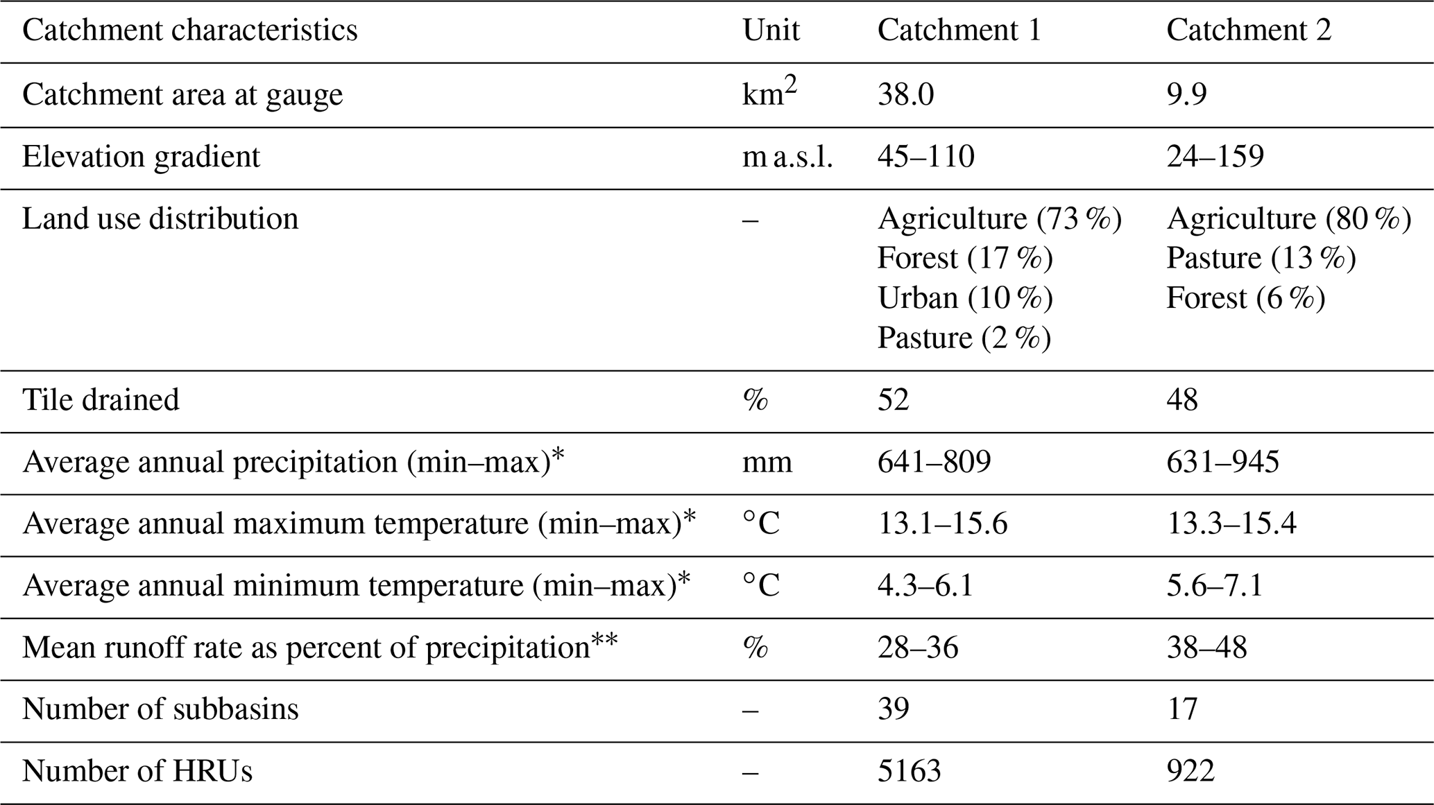
^∗ Time period: January 2008 to December 2013, ${}^{\ast \ast }$ time period: June 2010 to December 2013.

Model parameterization followed standard procedures considering information on climate, topography, soil, land use properties, agricultural management practices (including pesticide applications), and tile drain locations. SWAT offers a range of algorithms representing hydrological processes. Based on experience and understanding of the catchment characteristics, the Hargreaves potential evaporation method and the evaporation-based daily curve number adjustment method were chosen. Pre-calibration settings of hydrologic parameters included the adjustment of heat units to ensure crops develop completely and the adjustment of channel roughness to account for vegetated, small channels. Application data on respective crops were available with approximate amounts and timing for C1 and as field-specific applications for C2. The pesticide's average application rates are 221 g ha⁻¹ in C1 and 462 g ha⁻¹ in C2. Metabolite release in the soil was parameterized to account for metabolite formation in the soil profile using pseudo chemical applications for both model versions. Pesticide-related algorithms and parameters updated prior to calibration included pesticide in-stream processes such as burial and volatilization, which were turned off due to the low Koc, Henry's law constant, and vapor pressure of both chemicals and the short travel time in the two catchments.

A multi-metric calibration was conducted combining visual comparison and multiple performance metrics for both streamflow and concentration of the chemicals using the modified SWAT code. The calibration was conducted separately and iteratively for streamflow and pesticide concentrations (i.e., no multi-objective function combining streamflow and pesticide metrics was used). The entire record of observed chemical concentrations was selected as the calibration period and a second independent validation period was not selected. This is a common approach used for hydrologic and pesticide model calibration when the observed data period is relatively short (Daggupati et al., 2015). The models for the two watersheds were first calibrated using the modified code and then both model versions (original and modified) were run using the same parameters. This is not meant to be a completely “equitable” model performance comparison, but to show the differences between the two versions. A list and description of the calibration parameters and the processes they are associated with is provided in Table 2. A parameter is included in the table if it was changed in at least one of the catchments.

Table 2 Calibration parameters with initial value and calibrated end value (changed values in bold).

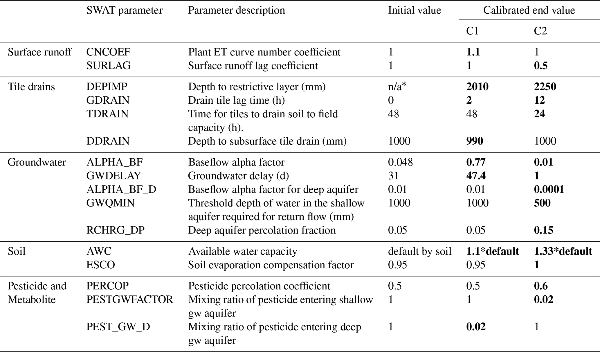
^* n/a stands for not applicable.

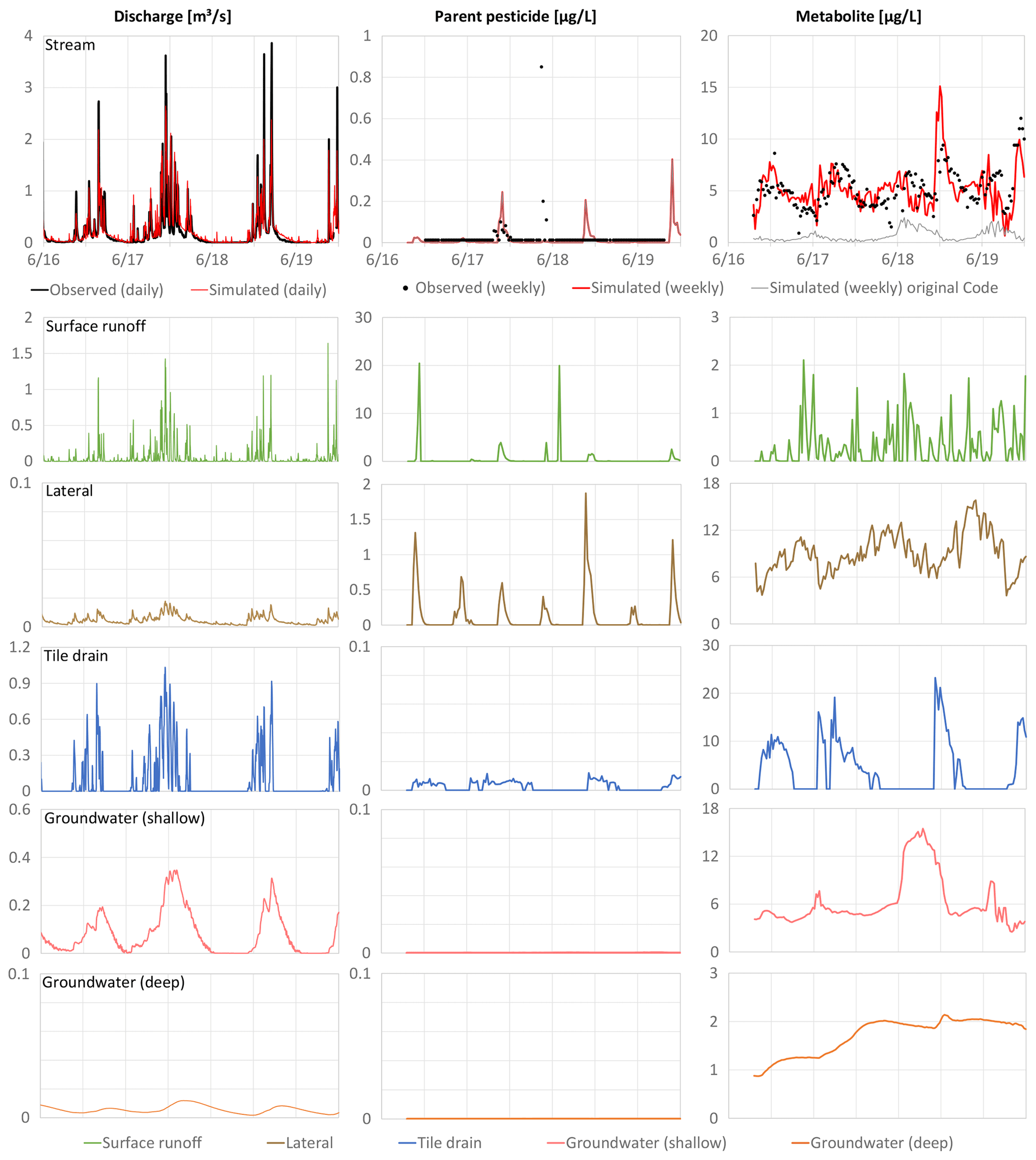
Figure 2 Catchment 1 (C1) time series (June 2016–December 2019) for observed and simulated discharge, parent pesticide, metabolite in streamflow and simulated time series for all flow components.

Figure 3 Catchment 2 (C2) time series (June 2010–December 2013) for observed and simulated discharge, parent pesticide, metabolite in streamflow and simulated time series for all flow components.

Figures 2 and 3 show discharge, pesticide, and metabolite concentrations (columns) for the different flow components (rows) for C1 and C2, respectively. The hydrologic calibration led to a good visual agreement between observed and simulated discharge and good to very good performance statistics with daily NSE values of 0.76, 0.63 and PBIAS of 6.6 %, 1.8 % in C1 and C2, respectively. The pesticide and metabolite concentrations in streamflow simulated with the original SWAT code (gray lines) and the modified code (red lines) are shown in Figs. 2 and 3. The original and modified SWAT pesticide simulations returned similar results and a good fit between modeled and observed concentrations was achieved. However, C1 was characterized by very few detections above the level of quantification and the highest observed pesticide peak could not be reproduced by both models. In C2, reported point source inputs of the pesticide occurred (likely due to mistreatment of the product) which are not included in the model; this leads to discrepancies between simulated and observed concentrations. The metabolite dynamics and magnitudes cannot be reproduced by the original SWAT code in both catchments, but are very well represented by the modified code, emphasizing the importance of the subsurface transport processes for the metabolite.

The contribution of the different flow components to discharge is similar in both catchments where surface runoff has the highest impact on peak flows. Tile drains are relevant mostly in the wetter months and shallow groundwater shows a clear seasonal dynamic with lowest flow values in summer. Lateral flow and deep groundwater flow have low contributions. The deep groundwater aquifer, however, sustains the flows in the summer periods. The modified SWAT code allows the output of concentrations in all flow components. They show a similar pattern in both catchments where surface runoff and lateral flow are the only flow components with significant concentrations. All simulated pesticide peaks can be attributed to surface runoff events as comparably high pesticide concentrations in streamflow coincide with a significant runoff event. Pesticide concentrations in lateral flow are also significant, but the contribution of lateral flow to total streamflow is low, and loadings in lateral flow are therefore significantly diluted when entering the stream. The concentrations of the metabolite in streamflow have a comparable magnitude in C1 and C2 (maximum between 10 to 15 µg L⁻¹) and the dynamics of the concentrations in the transport components have a similar pattern in both catchments. Concentrations in lateral flow fluctuate, but are always greater than zero, indicating a constant presence of the metabolite in the soil. This can also be seen in the high tile drain concentrations that lead to substantial metabolite contributions when tile flow occurs. The metabolite is also permanently present in the groundwater, which is a significant transport pathway.

These results show that the fast flow components are responsible for the pesticide concentrations in streamflow. For the metabolite, a single most important transport process cannot be identified and a complex interplay between multiple transport pathways is responsible for the concentration dynamics and magnitude: lateral flow and shallow groundwater flow are the most important input pathways in summer during low flow conditions and tile drain flow during autumn and winter. Surface runoff and deep groundwater flow have negligible contributions.

4 Summary and conclusion

The SWAT model code was extended to simulate pesticide transport through tile drains and two groundwater layers. All subroutines and a compiled executable are provided in the electronic supplements to this technical note. For applying the updated model, minor changes must be made to the standard SWAT input files with two additional parameters in one input file.

The application of the implemented code in the two case study catchments demonstrates the advantages to simulating pesticide transport through tile drains and groundwater flow. The actual concentrations in the respective transport pathways and water balance components are available over time; this is important information to assess environmental fate and transport processes. It is also apparent that the complex temporal interplay between all flow components, including tile and groundwater flow, is needed to sufficiently simulate concentrations of metabolites and other chemicals with similar properties in streamflow. Visualizing the pesticide and metabolite concentration in all flow components improves the understanding of the origin of the chemicals. This supports a more targeted calibration of the models and provides important information to develop best management practices to mitigate potential contamination of surface and groundwater.

The developed software fills a gap in watershed-scale pesticide modeling. The code refinements were made available to the SWAT development team and will potentially be included in a future official revision of the SWAT model. The next version of the SWAT model, called SWAT+ (Bieger et al., 2017), will include the simulation of pesticides in all hydrological flow pathways and a direct simulation of metabolite formation using a first-order decay function. However, while scientists and watershed managers are in the process of transitioning to SWAT+ and its supporting interfaces become available, the extended SWAT version is a valuable tool for risk managers and exposure modelers.