Estimation of hydraulic conductivity functions in karst regions by particle swarm optimization with application to Lake Vrana, Croatia

To examine the effectiveness of various technical solutions for minimizing the adverse effects of saltwater intrusion in Lake Vrana, Croatia, a reliable mathematical model for describing the exchange of fresh- and saltwater between the lake and its surroundings is needed. For this purpose, a system of two ordinary and nonlinear differential equations is used. The variable coefficients represent hydraulic conductivity functions that are used to quantify groundwater flow and should be appropriately estimated by relying on data obtained by in situ measurements. In the abstract space of all possible hydraulic conductivity functions, the method of particle swarm optimization was used to search for functions which will minimize the difference between the predicted (modeled) and realized (measured) water surface elevation in the lake through the time span of 6 years (which includes relevant hydrological extremes – droughts and floods). The associated procedure requires the parameterization of conductivity functions which will define the number of dimensions of the search space. Although the considered mass exchange processes are significantly nonlinear, and the parametrization of hydraulic conductivity functions can define a search space with a relatively large number of dimensions (60 dimensions were used to estimate the hydraulic conductivity functions of Vrana lake), the presented example confirms the effectiveness of the proposed approach.

1 Introduction

Water management in karst areas near the sea usually requires modeling water quantity and quality under different hydrological conditions (Bakalowicz, 2005). Karst area water resources are endangered by global littoralization processes and also by negative anthropogenic impacts through which the requirements for freshwater quantities are progressively increasing. At the same time, natural processes manifested through climate change also negatively affect karst water resources by (i) raising sea levels (which can endanger freshwater quality), (ii) reducing precipitation (on the basis of which such sources are fed), and (iii) rising air temperatures (increasing the amount of freshwater evaporation). All this obliges us to prioritize the protection of such water resources, which in part requires the mathematical modeling of water flow in karst conduits. In this context, the attention in the paper is given to a specific problem of estimating the unknown hydraulic conductivity functions by which the groundwater flow in karst conduits is computed in the framework of semi-distributed lumped karst models. The related computational framework is well established (Gunn, 1986; Bergström and Forsman, 1973) and, in many cases, successfully implemented (Fiorillo, 2011; Gàrfias et al., 2007; Fleury et al., 2007). Moreover, the semi-distributed lumped karst models is particularly interesting in the case of poorly characterized karst aquifers. By representing the karst aquifer as a finite number of interconnected reservoirs (also known as hydrological compartments), the flow through karst conduits is represented as a consequence of the difference in water levels in interconnected reservoirs. In order to quantify the achieved water flow, the related heterogeneous hydrogeological properties are usually homogenized and described by parameters dependent on flow characteristics such as water level. As a consequence, the hydrological data are not spatially distributed, and the simplified karst aquifer description relies on model calibration.

If the continuous time series of relevant hydrological data is known in advance (which was the case for the considered research area), then the application of the principle of conservation of mass is very attractive for modeling the time change in water level in karst region. In this case, the dynamic behavior of such systems is described by a nonlinear first-order ordinary differential equation (ODE) with variable coefficients (or a system of ODEs). The variable coefficients should be determined from model calibration. Since the system is described by nonlinear ODEs, the calibration methods are based on the assumption that a karst aquifer represented by a connected series of linear reservoirs cannot be used. In these cases, the calibration of the semi-distributed lumped karst model can be very challenging. Although, in such circumstances, the model calibration procedure usually begins with a naive trial and error approach (Rimmer and Salingar, 2006), which is effective only in rare cases. Namely, the model variables are usually very sensitive to changes in calibration functions (which depend on model variables). As an alternative, several methods have been developed for this purpose. A commonly used approach is based on a statistical and correlation time series analyses of the measured hydrological data related to karst aquifers (Dubois et al., 2020). However, in cases of strongly nonlinear dependencies, it is inevitable to base the calibration process on some auto-correction method which relies on a definition of efficiency, like the Nash–Sutcliffe efficiency measure, or some modifications thereof (Charlier et al., 2012).

Regardless of the adopted approach, the success of the model calibration can depend on the number of parameters that are subject to calibration. Namely, for a semi-distributed lumped karst model in which the exchange of water between an interconnected karst region is modeled by more than one ODE, different values of calibration parameters can result in a similar model prediction (Wheater et al., 2022; Ye et al., 1997). In other words, there may be multiple solutions (known as multimodality), which consequently leads to unreliability in the physical interpretation of the model parameters (Beven, 2006). In order to reduce the influence of over-parameterization and obtain a unique solution, the number of all possible solutions should be reduced by introducing additional constraint conditions imposed on the calibration parameters. If no generic property can be defined for a particular calibration parameter by which the constraint condition can be formulated, then the additional constraint conditions are obtained through an analysis of the relative relationships between the available hydrological time series (which is often carried out by correlation and cross-correlation analyses). In other words, solving multimodal problems most often requires the application of an algorithm for pattern recognition in the available hydrological time series. For this reason, it should not be surprising that artificial neural networks (Kurtulus and Razack, 2010; Hu et al., 2008; Coppola et al., 2003; Coulibaly et al., 2001) and different machine learning methods (Wunsch et al., 2022) have found their application in the calibration of semi-distributed lumped karst models. However, the mentioned approaches are not that suitable in cases where the constraint conditions are known in advance and are given in the form of mathematical inequalities (as was the case in this paper). In such cases, it is opportune to treat the calibration of model parameters as an optimization problem (Beasley et al., 2012) in which multimodality is commonly encountered. In such circumstances, the calibration of model parameters requires the definition of an objective function that is dependent on design variables (i.e., model parameters). Since the objective function is usually defined as a measure of difference between the considered predicted value and the one obtained by field measurements, the calibration of model parameters is reduced to its minimization. For this purpose, the domain of the objective function is searched in an iterative fashion. Unless a specific search (local search) of the domain of the objective function is expected, the parameters of a karst model can be effectively calibrated by genetic algorithms (Lu et al., 2018). For more demanding optimization problems, in which it is expected that the objective function has many local minima permeating throughout the entire domain of the objective function (multimodality), both a global and a local search is necessary. In these situations, the bio-inspired algorithm known as particle swarm optimization (PSO method) is more suitable because it is based on a simultaneous local and global search of the domain of the objective function (Qian et al., 2019), and so, it is very attractive for solving multimodal problems (Özcan and Yilmaz, 2007). Moreover, this approach has previously been successfully applied to calibrate groundwater flow models in alluvial aquifers (Haddad et al., 2013; Mahmoud et al., 2021) and also for calibrating flow parameters in environmental models (Zambrano-Bigiarini and Rojas, 2020). In order to examine the application of the PSO method and indicate the possibilities it offers in the contest of karst modeling, it was applied to the estimate the hydraulic conductivity functions used for modeling the exchange of fresh- and saltwater in Lake Vrana, Croatia.

2 Study area

The proposed procedure for estimating hydraulic conductivity functions has been successfully applied in quantifying water flow through the bed of Lake Vrana (which is the largest natural lake in Croatia, with a water surface area of more than 30 km²). Lake Vrana is a cryptodepression separated from the Adriatic Sea by an narrow karst ridge (width varying from 0.8 to 2.5 km) through which fresh- and saltwater can be exchanged. The exchange of water is bidirectional, and the orientation of the established groundwater flow, which is important in the context of preserving freshwater quality, depends on the achieved pressure gradient along karst conduits. In this regard, it is important to note that the Lake Vrana water level varied from 0.03 to 2.25 m a.s.l. (above sea level) in the time span from 1948 to 2010 (Rubinić and Katalinić, 2014). Although the lake water level was above the sea level for the entire time, the risk of salinization can be recognized by (i) the fact that the average lake water level in the specified period was 0.83 m a.s.l. and (ii) taking into account that the pressure gradient also depends on the relative deference in fresh- and saltwater density (so that the saltwater intrusion is established even at equal water levels). Moreover, in August 2012, due to unfavorable hydrological trends (attributed to climate change), the depth of the lake water was only 30 cm, and a very high salinity of as much as 17 ‰ was recorded. This was a consequence of site specifics, namely the very close proximity of the sea and the relatively shallow water in the lake. Furthermore, it should be noted that the lake bed at the deepest point is only 3 m b.m.s.l. (below mean sea level), and thus the lake is under constant danger of salinization (Rubinić, 2014).

In addition to the information previously mentioned, it should be emphasized that the quality and quantity of water are also significantly affected by the presence of the Prosika channel, through which fresh- and saltwater can be exchanged by (i) surface flow through the channel and (ii) groundwater flow through the porous channel bed. The Prosika channel was originally dug in 1770 to attain new agricultural areas near Lake Vrana that needed protection from seasonal flooding. With a total length of 770 m and a trapezoidal cross section, with a channel bottom width of 8 m, the Prosika channel connects Lake Vrana and the Adriatic Sea. The location of Lake Vrana, the Prosika channel, and the Adriatic Sea is shown in Fig. 1. Throughout history, the Prosika channel has undergone several geometric adaptations which led to weir of fixed height and a crest at 0.41 m a.s.l. on the downstream side of the channel (which has the role of separating fresh- and saltwater in case the sea is at a lower elevation). However, the fixed crest height, which was originally determined to be a compromise between maximizing the channel flow area during flooding and minimizing the channel flow area during saltwater intrusion, is no longer adequate because in recent history the problem of saltwater intrusion has repeatedly arisen.

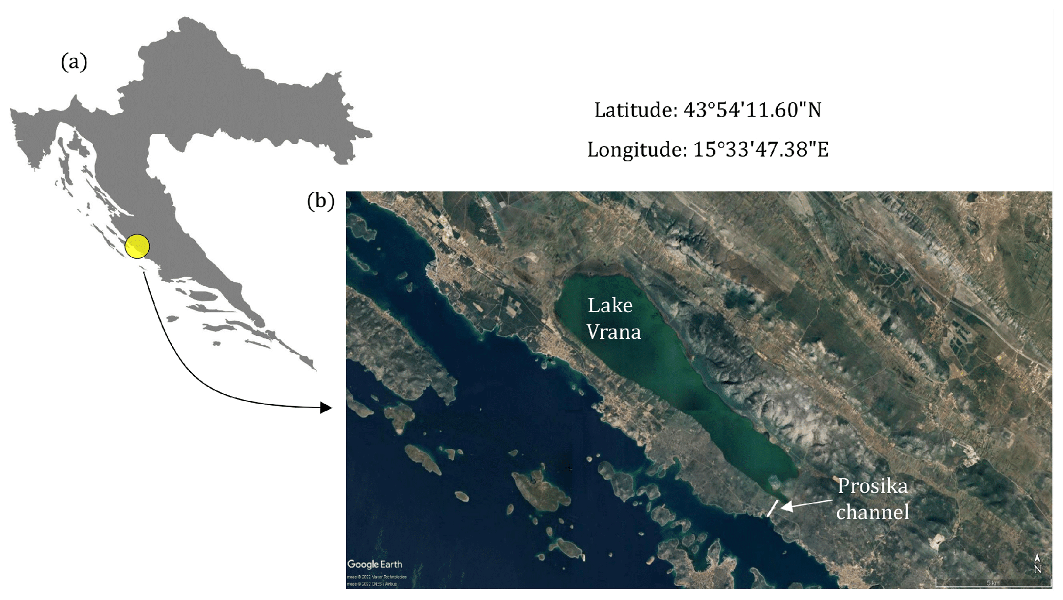
Figure 1 (a) Geographical position of Lake Vrana, Croatia, and (b) a satellite view of the lake with the marked area of the Prosika channel through which the exchange of fresh- and saltwater is conducted by surface water flow (depending on the established boundary conditions). Map data from Google Earth and image © 2022 Maxar Technologies and CNES/Airbus.

In order to reduce the negative consequences of salinization (or significantly reduce saltwater intrusion), it is necessary to intervene in the process of exchange of fresh- and saltwater in Lake Vrana by some technical solution. For this purpose, the adopted technical solution should (i) increase the storage time of freshwater in Lake Vrana (which is supplied only through precipitation and surface and groundwater flow from a karst aquifer) and (ii) reduce the intrusion of saltwater from Adriatic Sea (by surface water flow through the Prosika channel or groundwater flow thought the porous Prosika channel bed and Lake Vrana bed). Regardless of the adopted technical solution, the resulting effect must be quantified by comparing the volume of salt- and freshwater in Lake Vrana under different and relevant hydrological scenarios. For this purpose, it is necessary to formulate a mathematical model that can be used to simulate the exchange time of fresh- and saltwater in Lake Vrana under different hydrological conditions, which in turn requires a realistic description of the groundwater flow (while the surface flow through the Prosika channel can be modeled relatively easily). Thus, the modeling problem is reduced to defining the suitable hydraulic flow conditions in an unknown network of conduits in the surrounding karst aquifer.

Within the basin of Lake Vrana, a few groups of rocks can be recognized (Rubinić, 2014). First of all, these are Upper Cretaceous limestones (i.e., very permeable rocks within which an underground hydrographic network has been developed). On the other hand, it is also possible to determine the area within which the dolomites and limestones of the lower part of the Upper Cretaceous alternate, forming a medium permeable layer that can slow down the flow of underground water. Finally, a large part of the basin consists of impermeable or very poorly impermeable flysch deposits that in some places cause the formation of surface flows. For calibrating the model parameters, these surface flow components will be set based on known in situ measurements. On the other hand, the groundwater flow components, which are realized as a consequence of the developed hydrographic network in the Upper Cretaceous limestones, will be modeled using the semi-distributed lumped karst model, relying on the assumption of a fully turbulent flow.

3 Research method

The semi-distributed model or pipe flow model (Gill et al., 2021; Schmidt et al., 2014; Bailly et al., 2012; Thrailkill, 1974) was used to model the storage dynamics of Lake Vrana and its hydrogeological connectivity with the (i) surrounding karst basin (from which it is supplied with freshwater) and (ii) Adriatic Sea (where freshwater from Lake Vrana sinks). Accordingly, groundwater flow was modeled using the assumption of fully turbulent and partially saturated water flow through karst conduits in the phreatic and epihreatic zones (Shoemaker et al., 2008; Bonacci, 1993), neglecting Darcy's flow component. Under these assumptions, the karst conduit networks can be conceptualized as a system of connected pipelines so that the relevant hydraulic parameters are related through the Darcy–Weisbach equation by introducing hydraulic conductivity functions.

3.1 Hydraulic conductivity function

For an ideal conduit with a circular cross section, the Darcy–Weisbach equation can be written as follows:

$$\begin{array}{}\text{(1)}& h_a-h_b=\mathit{\lambda }{\displaystyle \frac{L}{D}}{\displaystyle \frac{{\stackrel{\mathrm{‾}}{v}}^{\mathrm{2}}}{\mathrm{2}g}},\end{array}$$

where h_a and h_b represent the pressure heads (L) at the opposite ends a and b of the conduit, λ is the Darcy's friction coefficient (1), L is the length of the conduit (L), D is the diameter of the conduit (L), $\stackrel{\mathrm{‾}}{v}$ is the average flow velocity (L T⁻¹), and g is the acceleration of gravity (L T⁻²).

The flow rate q_ab through the conduit can be obtained by multiplying the cross-sectional area A, with the average flow velocity $\stackrel{\mathrm{‾}}{v}$ from Eq. (1), thus introducing the flow model, as follows:

$$\begin{array}{}\text{(2)}& q_{ab}=\underset{c_{ab}\left(\mathrm{\Delta }{h}_{ab}\right)}{\underbrace{A\sqrt{{\displaystyle \frac{\mathrm{2}gD}{\mathit{\lambda }L}}}}}\sqrt{h_a-h_b},\end{array}$$

which can be generalized to generic flow conditions. Namely, the flow rate q_ab through the conduit can be related to the square root of a pressure head difference $\mathrm{\Delta }{h}_{ab}=h_a-h_b$ on the right-hand side by a proportionality factor c_ab (L${}^{\mathrm{5}/\mathrm{2}}$ T⁻¹), which describes the combined influence of the geometric and kinematic properties of the flow. Moreover, since both flow characteristic will be affected by the pressure head difference, c_ab can be interpreted as a hydraulic conductivity function with the argument Δh_ab. To generalize the flow model with respect to the flow direction, which can change depending on the sign of the pressure head difference Δh_ab, Eq. (2) can be rewritten as follows:

$$\begin{array}{}\text{(3)}& q_{ab}=\mathrm{sgn}\mathrm{\Delta }{h}_{ab}\cdot c_{ab}\left(\mathrm{\Delta }{h}_{ab}\right)\cdot \sqrt{\mathrm{|}{h}_a-h_b\mathrm{|}}.\end{array}$$

In order to include the dependence of a pressure gradient on the difference in water density at the conduit ends, the pressure head h_b in Eq. (3) should be modified by a factor r_ρ that represents the ratio between the density of the water ρ_b with the pressure head h_b and the density of water ρ_a with the pressure head h_a, which leads to the flow model, as follows:

$$\begin{array}{}\text{(4)}& q_{ab}=\mathrm{sgn}\mathrm{\Delta }{h}_{ab}\cdot c_{ab}\left(\mathrm{\Delta }{h}_{ab}\right)\cdot \sqrt{\mathrm{|}{h}_a-r_{\mathit{\rho }}{h}_b\mathrm{|}},\end{array}$$

where the hydraulic conductivity function c_ab(Δh_ab) should be estimated by inverse modeling (Li et al., 2018; Nematolahi et al., 2018), which means relying on the available data obtained from in situ measurements. It should be pointed out that the functions under consideration can be highly nonlinear due to the nonlinear effect of friction (for flow in pipes defined by the Colebrook equation) and, even more so, due to the change in the geometry of the conduit network that can vary as a function of surface water and groundwater level.

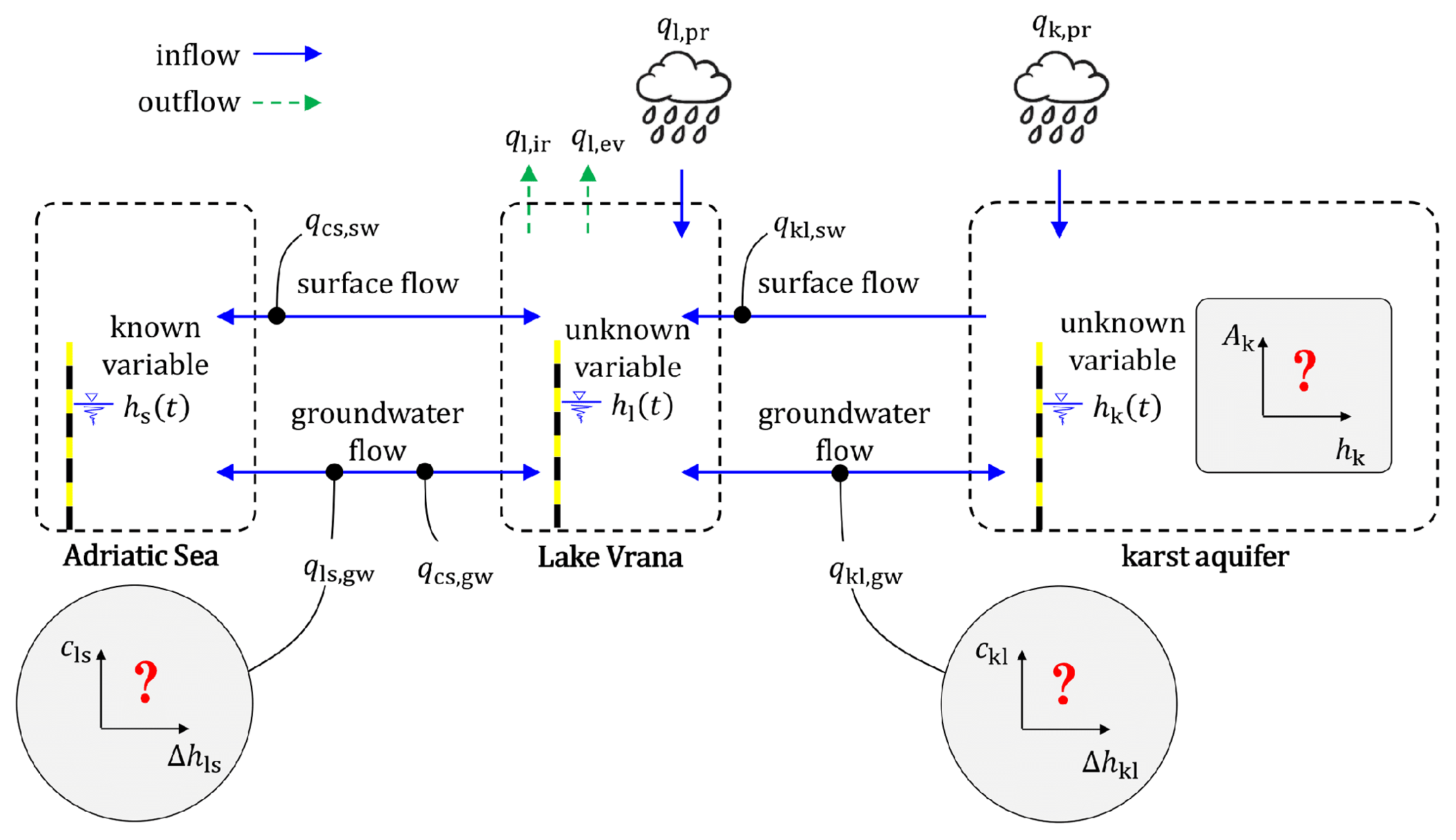
Figure 2 A conceptual model used to describe the storage dynamics of Lake Vrana and its hydrogeological connectivity with (i) Adriatic Sea and (ii) surrounding karst aquifer.

3.2 Conceptual model

The freshwater and seawater exchange between Lake Vrana and the Adriatic Sea, in addition to the exchange of freshwater between Lake Vrana and its surrounding karst aquifer, can be described by Eq. (4). For this purpose, the mathematical model must include three variables, namely the (i) sea level h_s, (ii) lake water level h_l, and (iii) karst groundwater level h_k. Within a given time domain, the change in sea level h_s, as described by function h_s(t) over time t, is given in advance, and the functions h_l(t) and h_k(t) will be treated as unknown quantities that will be approximated for the given initial and hydrological conditions. The corresponding semi-distributed lumped karst model will result in a system of three interconnected reservoirs that are introduced to conceptually represent the hydrological compartments of (i) the Adriatic Sea, (ii) Lake Vrana, and (iii) the karst aquifer. The relative relationship between the introduced hydrological compartments, with the corresponding degrees of freedom h_s, h_l and h_k, and their interconnected flow components are illustrated in Fig. 2.

Apart from the groundwater flow components, the conceptual model should also include the exchange of water between the introduced hydrological compartments achieved by surface water flow. Namely, the surface water component plays an important role because it feeds Lake Vrana with freshwater (like the groundwater flow component from the karst aquifer). On the other hand, the surface flow component between Lake Vrana and the Adriatic Sea, achieved through the Prosika channel, can adversely affect the quantity and quality of water in Lake Vrana. Namely, in the case of downstream flow (from the lake towards the sea), the quantity of freshwater in Lake Vrana is reduced, thus increasing the relative difference in the variables h_s and h_l in the unfavorable direction. Otherwise, in the case of upstream flow (from the sea towards the lake), the percentage of saltwater in the lake will increase. These situations, and in the case in which there is no surface flow through the Prosika channel, will depend on the boundary conditions at the channel ends, which should be included in the corresponding mathematical model.

3.3 Mathematical model

To formulate a formal mathematical representation of the previous conceptual model, a principle of mass conservation can be applied to reservoirs introduced to model the lake water level h_l and groundwater level h_k in the surrounding karst aquifer. Accordingly, a principle of mass conservation for groundwater in the karst aquifer requires the following:

$$\begin{array}{}\text{(5)}& A_{\mathrm{k}}\left(h_{\mathrm{k}}\right){\displaystyle \frac{\mathrm{d}{h}_{\mathrm{k}}}{\mathrm{d}t}}=\underset{\mathrm{given}}{\underbrace{q_{\mathrm{k},\mathrm{pr}}}}-\underset{q_{\mathrm{kl},\mathrm{gw}}}{\underbrace{\mathrm{\Delta }{h}_{\mathrm{kl}}\cdot c_{\mathrm{kl}}\left(\mathrm{\Delta }{h}_{\mathrm{kl}}\right)\cdot \sqrt{\mathrm{|}{h}_{\mathrm{k}}-h_{\mathrm{l}}\mathrm{|}}}},\end{array}$$

where the function A_k(h_h) relates the groundwater level h_k (L) to the corresponding horizontal-section area A_k (L²) of the karst conduit networks, q_k,pr represents the freshwater inflow from precipitation (L³ T⁻¹), and q_kl,qw is the groundwater flow component between the karst conduit networks and Lake Vrana, as calculated by Eq. (4), where c_kl(Δh_kl) denotes the corresponding hydraulic conductivity function with the argument defined as $\mathrm{\Delta }{h}_{\mathrm{kl}}=h_{\mathrm{k}}-h_{\mathrm{l}}$. It should be highlighted that the function A_k(h_h) denotes the arrangement of the cross-sectional surface areas of crack openings in the karst environment with respect to groundwater level and thus includes the surfaces of karst conductors, caves, caverns, etc. Like hydraulic conductivity functions, this function is also unknown in advance and should be obtained by model calibration which respects the characteristic of a progressive decrease with the rise in groundwater level (due to the dissolution process that creates larger openings in the deeper parts of the karst).

Similarly, the principle of mass conservation for Lake Vrana requires the following:

$$\begin{array}{}\text{(6)}& \begin{array}{rl}{A}_{\mathrm{l}}\left(h_{\mathrm{l}}\right){\displaystyle \frac{\mathrm{d}{h}_{\mathrm{l}}}{\mathrm{d}t}}& =\underset{\mathrm{given}}{\underbrace{q_{\mathrm{kl},\mathrm{sw}}+q_{\mathrm{l},\mathrm{pr}}-q_{\mathrm{l},\mathrm{ir}}-q_{\mathrm{l},\mathrm{ev}}}}+q_{\mathrm{kl},\mathrm{gw}}\\ & -q_{\mathrm{cs},\mathrm{sw}}-\underset{q_{\mathrm{cs},\mathrm{gw}}}{\underbrace{\mathrm{\Delta }{h}_{\mathrm{cs}}\cdot c_{\mathrm{cs}}\left(\mathrm{\Delta }{h}_{\mathrm{cs}}\right)\cdot \sqrt{\mathrm{|}{h}_{\mathrm{c}}-r_{\mathit{\rho }}{h}_{\mathrm{s}}\mathrm{|}}}}\\ & -\underset{q_{\mathrm{ls},\mathrm{gw}}}{\underbrace{\mathrm{\Delta }{h}_{\mathrm{ls}}\cdot c_{\mathrm{ls}}\left(\mathrm{\Delta }{h}_{\mathrm{ls}}\right)\cdot \sqrt{\mathrm{|}{h}_{\mathrm{l}}-r_{\mathit{\rho }}{h}_{\mathrm{s}}\mathrm{|}}}},\end{array}\end{array}$$

where the function A_l(h_l) relates the lake water level h_l (L) to the corresponding water surface area A_l (L²) in Lake Vrana (known by in situ measurements), q_kl,sw represents the surface water inflow (L³ T⁻¹), q_l,pr is the freshwater inflow from precipitation on water surface area A_l (L³ T⁻¹), q_l,ir is the freshwater outflow from irrigation (L³ T⁻¹), q_l,ev is the freshwater outflow from evaporation (L³ T⁻¹), q_cs,sw and q_cs,gw are the surface water and groundwater flow components achieved between the Prosika channel and the Adriatic Sea (L³ T⁻¹), and q_ls,gw is the groundwater flow component between Lake Vrana and the Adriatic Sea (L³ T⁻¹). It should be noted that the first four terms on the right-hand side are known from in situ measurements.

As in Eq. (5), the groundwater flow components in this case are computed by Eq. (4), so that c_cs(Δh_cs) and c_ls(Δh_ls) represent the hydraulic conductivity functions for groundwater flow components achieved between the (i) Prosika channel and Adriatic Sea and (ii) Lake Vrana and the Adriatic Sea. However, it is opportune to note that the argument $\mathrm{\Delta }{h}_{\mathrm{ls}}=h_{\mathrm{l}}-h_{\mathrm{s}}$ can be explicitly computed and that the argument Δh_cs, which represents the difference in water level in the Prosika channel h_c and sea level h_s, requires a modeling procedure through which the water surface profile h_s(s) along the channel station s is computed for a given set of boundary conditions. For this purpose, a standard step method was used. Moreover, it should be noted that the sinking flow component along the channel, introduced in Eq. (6) by the term q_cs,gw, requires the hydraulic conductivity function c_cs(Δh_cs), which was set to be linear so that the difference in water level Δh_cs=0.8 corresponds to the value of c_cs=0.5 m${}^{\mathrm{5}/\mathrm{2}}$ s⁻² (as established by in situ measurements).

By the principle of mass conservation, Eqs. (5) and (6) form a system of two nonlinear ordinary differential equations that can be used to describe the relationship between quantities h_k and h_s for a given set of initial conditions and known hydrological parameters over the considered time domain. However, to obtain reliable solutions, there are three functions that should be obtained by inverse modeling, which means relying on the following known data obtained by in situ measurements: (i) c_kl(Δh_kl), (ii) c_ls(Δh_ls), and (iii) A_k(h_h). However, as the functional relationship between the groundwater flow q and pressure gradient is nonlinear, as given by Eqs. (3) and (4), it should be emphasized that even a small change in one of the estimated hydraulic conductivity functions will result in a relatively large difference in the predicted function h_l(t). Moreover, the deviation between the predicted and realized lake water levels, at any point in time, can be related to the volume of water that is transferred to the rest of the time domain, so deviations between predicted and measured lake water levels can only increase over time (because the mathematical model is based on the principle of mass conservation). For this reason, the problem of estimating the hydraulic conductivity functions is usually very complex (especially in large time domains that need to take different hydrological situations into account ).

3.4 Particle swarm optimization

The unknown functions are estimated by model calibration (Kuok and Chiu, 2012; Zambrano-Bigiarini and Rojas, 2013), which is performed in an iterative fashion, relying on available hydrological data. The procedure requires a representative time domain (with hydrological extremes) in which all the relevant data are well documented by in situ measurements. In that case, the mathematical model can be used to predict the function h_l(t) under the same hydrological conditions that led to the change in the lake water level ${\widehat{h}}_{\mathrm{l}}$ observed by in situ measurements and described by the function ${\widehat{h}}_{\mathrm{l}}\left(t\right)$. In that case, the assumed functions c_kl(Δh_kl), c_ls(Δh_ls) ,and A_k(h_h), which can be interpreted as design functions, are validated by comparing the predicted h_l(t) and achieved ${\widehat{h}}_{\mathrm{l}}\left(t\right)$ change in the lake water level h_l. The difference under consideration can be measured by a function G, defined as the sum of squared differences $h_{\mathrm{l}}\left(t_n\right)-{\widehat{h}}_{\mathrm{l}}\left(t_n\right)$, performed over a finite number of points t_n in the given time domain (where n ranges from 0 to n_Δt). Accordingly, the shaping of the design functions can be viewed as an optimization problem that requires the minimization of function G which, in that case, represents the objective function.

Since the optimization procedure in the proposed methodology is conducted numerically (not analytically), the design functions are represented by a series of function values equidistantly distributed between the minimal and maximal values of each design function domain. These discrete values, used to approximate the design functions, are collected in a vector x^(e) and updated after each evaluation step (e).

In recent years, modern stochastic global optimization methods have been successfully applied in many difficult real-world problems. One such optimization method is particle swarm optimization (PSO), which has been employed in several hydrological modeling problems. In the PSO method (Clerc, 2010), the search space of all possible design functions is explored by n_p agents called particles, each with their own iteratively updated set of design variables ${\mathit{x}}_{\mathrm{p}}^{\left(\mathrm{e}\right)}$.

In accordance with the above, particle p in an evaluation step (e) evaluates its design vector ${\mathit{x}}_{\mathrm{p}}^{\left(\mathrm{e}\right)}$ by using the objective function as follows:

$$\begin{array}{}\text{(7)}& G\left(\mathit{x}\right)=\sum _{n=\mathrm{0}}^{n_{\mathrm{\Delta }t}}{\left(h_{\mathrm{l}}\left(\mathit{x},t_n\right)-{\widehat{h}}_{\mathrm{l}}\left(t_n\right)\right)}^{\mathrm{2}},\end{array}$$

where the function h_l(x,t_n) represents the model prediction for design variables

$$\begin{array}{}\text{(8)}& {\mathit{x}}_{\mathrm{p}}^{\left(\mathrm{e}\right)}=\left\{\begin{array}{c}{c}_{\mathrm{kl}}\left(\mathrm{\Delta }{h}_{\mathrm{kl},\min }\right)\\ \mathrm{⋮}\\ c_{\mathrm{kl}}\left(\mathrm{\Delta }{h}_{\mathrm{kl},\max }\right)\\ c_{\mathrm{ls}}\left(\mathrm{\Delta }{h}_{\mathrm{ls},\min }\right)\\ \mathrm{⋮}\\ c_{\mathrm{ls}}\left(\mathrm{\Delta }{h}_{\mathrm{ls},\max }\right)\\ A_{\mathrm{k}}\left(h_{\mathrm{k},\min }\right)\\ \mathrm{⋮}\\ A_{\mathrm{k}}\left(h_{\mathrm{k},\max }\right)\end{array}\right\}.\end{array}$$

After evaluating all vectors ${\mathit{x}}_{\mathrm{p}}^{\left(\mathrm{e}\right)}$ in the current evaluation step (e), the vectors ${\mathit{x}}_{\mathrm{p}}^{(\mathrm{e}+\mathrm{1})}$ in the next evaluation step (e+1) are computed by kinematic analogy, as follows:

$$\begin{array}{}\text{(9)}& {\mathit{x}}_{\mathrm{p}}^{(\mathrm{e}+\mathrm{1})}={\mathit{x}}_{\mathrm{p}}^{\left(\mathrm{e}\right)}+{\mathit{v}}_{\mathrm{p}}^{(\mathrm{e}+\mathrm{1})},\end{array}$$

where v_p can be interpreted as velocity vector of particle p.

The crucial element of PSO is related to the computation of the velocity vector ${\mathit{v}}_{\mathrm{p}}^{(\mathrm{e}+\mathrm{1})}$, which is inspired by the movements of swarms in a collective search of some biological need (e.g., food). For this purpose, particle movement is affected by three components, including (i) the inertial component, which describes the tendency to preserve the current direction and speed of motion, (ii) a component of self-confidence that describes the tendency to explore the search space on the basis of personal search experience (particle memory influence), and (iii) a component of collective influence that describes the attraction of the very best solution found among the members of the swarm informing the particle in question (swarm memory influence). This collective influence is most often implemented as the influence of the information of the best solution found by the entire swarm; i.e., for the purpose of information sharing, the swarm is understood to be operating as a fully connected graph. Therefore, the velocity vector ${\mathit{v}}_{\mathrm{p}}^{\left(\mathrm{e}\right)}$ for each particle p can be updated according to the given description that can be mathematically represented by the following:

$$\begin{array}{}\text{(10)}& \begin{array}{rl}{\mathit{v}}_{\mathrm{p}}^{(\mathrm{e}+\mathrm{1})}& =\underset{\mathrm{inertia}}{\underbrace{w\cdot {\mathit{v}}_{\mathrm{p}}^{\left(\mathrm{e}\right)}}}+\underset{\mathrm{particle}\mathrm{memory}\mathrm{influence}}{\underbrace{c_{\mathrm{1}}\cdot {\mathit{r}}_{\mathrm{1}}\circ \left({\mathit{x}}_{\mathrm{p},\mathrm{best}}^{\left(\mathrm{e}\right)}-{\mathit{x}}_{\mathrm{p}}^{\left(\mathrm{e}\right)}\right)}}\\ & +\underset{\mathrm{swarm}\mathrm{memory}\mathrm{influence}}{\underbrace{c_{\mathrm{2}}\cdot {\mathit{r}}_{\mathrm{2}}\circ \left({\mathit{x}}_{\mathrm{g},\mathrm{best}}^{\left(\mathrm{e}\right)}-{\mathit{x}}_{\mathrm{p}}^{\left(\mathrm{e}\right)}\right)}},\end{array}\end{array}$$

where w is the dimensionless inertia parameter, c₁ and c₂ are dimensionless parameters used to describe the relative importance between the influence of particle memory and swarm memory, respectively, r₁ and r₂ are random vectors with components taken from a uniform statistical distribution between 0 and 1 and introduced to replicate the stochastic components of particles movement, ${\mathit{x}}_{\mathrm{p},\mathrm{best}}^{\left(\mathrm{e}\right)}$ is the vector of the design variables in the history of particle p, by which the objective function G reaches the minimal value (local optimum vector), ${\mathit{x}}_{\mathrm{g},\mathrm{best}}^{\left(\mathrm{e}\right)}$ is the vector of the design variables extracted from the search history of all particles by which the objective function reaches the so-far-established minimum (global optimum vector), and ∘ denotes the Hadamard product. After each particle evaluation, a check for updating the vectors ${\mathit{x}}_{\mathrm{p},\mathrm{best}}^{\left(\mathrm{e}\right)}$ and ${\mathit{x}}_{\mathrm{g},\mathrm{best}}^{\left(\mathrm{e}\right)}$ is performed. From the assumed initial position ${\mathit{x}}_{\mathrm{p}}^{\left(\mathrm{0}\right)}$ and velocity ${\mathit{v}}_{\mathrm{p}}^{\left(\mathrm{0}\right)}$ for all particles p, the optimization algorithm given by Eqs. (9) and (10) is repeated in an iterative fashion until the objective function G, for design variables ${\mathit{x}}_{\mathrm{p}}^{\left(\mathrm{e}\right)}$, yields a value lower than some predefined convergence limit or some other stopping criteria is achieved.

It should be noted that, for the problem under consideration, there are some constraints that can be superposed to the unknown functions c_kl(Δh_kl), c_ls(Δh_ls), and A_k(h_h) by reducing the search space and consequently increasing the efficiency of the optimization algorithm. Namely, as a consequence of the relation between the pressure gradient and discharge, the values of functions c_kl(Δh_kl) and c_ls(Δh_ls) must increase as Δh_kl and Δh_ls increase. In other words, functions c_kl(Δh_kl) and c_ls(Δh_ls) are monotonically increasing functions. On the other hand, a similar condition can be applied to function A_k(h_h). Moreover, it is reasonable to expect that the aquifer in consideration contains caves and caverns formed by limestone dissolution, underground water currents, and loads from upper karst deposits. Also, it is usually reasonable to assume that the volume of the caves and caverns increases with the aquifer depth, so that the condition of monotonicity in the growth of A_k(h_h) can be used for each of the n points used to represent the corresponding function values.

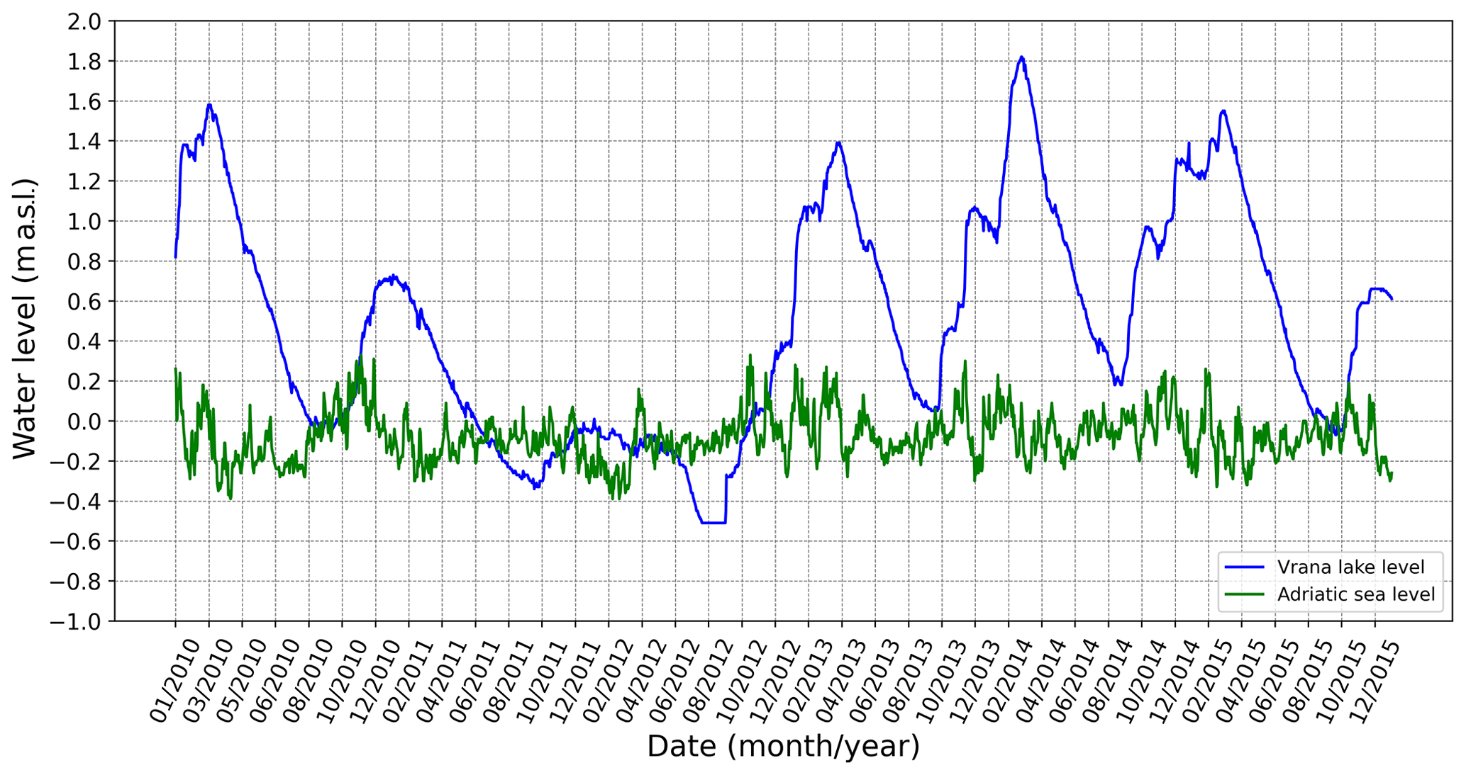
Figure 3 Measured lake water level and sea level in the time domain from early 2010 to late 2015. It should be noted that, in August 2011 and 2012, the sea level was above the lake water level, and so the intrusion of saltwater was significant. In addition, the lake water levels after these events should be viewed in the context of the weir crest at 0.41 m a.s.l.to identify the overflow during flood waves.

4 Results

The presented methodology was applied for the estimation of design functions c_kl(Δh_kl), c_ls(Δh_ls), and A_k(h_h) found in the previously presented mathematical model given by Eqs. (5) and (6) and developed for modeling the fresh- and saltwater exchange in Lake Vrana. Since the resulting computational algorithm is based on an iterative procedure by which the calibration of design functions is performed, it is appropriate to calibrate them for a relatively long and representative time domain within which hydrological extremes are present. For this purpose, the time domain from the beginning of 2010 to the end of 2015 was chosen to calibrate the subject design functions. This means that this time domain contains not only the previously mentioned case of extremely low lake water levels but also several cases of flood waves. These extreme events can be recognized in Fig. 3, which shows the measured lake water level and sea level. The variability in the hydrological conditions is necessary to reduce the multimodality of the optimization problem; i.e., this is in order to reduce the search space of the design functions that must be uniquely defined and ensure the agreement of modeled and measured lake water levels for dry and wet periods. The calibration process requires that, in the selected time domain, all the relevant hydrological and other data present in the corresponding mathematical model (terms on the right-hand side of the differential equations) must be known by in situ measurements (as is known in the case of Lake Vrana).

From the computational point of view, it should be noted that such large time domains require stable numerical integration, and therefore, the system of ordinary differential equations given by Eqs. (5) and (6) was solved by applying an implicit numerical scheme. On the other hand, it should also be noted that there are physical circumstances that can influence the choice of time step. In the present case, for example, the size of the time step is conditioned by the sea level dynamics illustrated in Fig. 3. In other words, the estimation of the design functions must be carried out to take into account the changes in groundwater flows that occur between Lake Vrana and the Adriatic Sea (the same as between the Prosika channel and Adriatic Sea) within 1 d as a result of changes in sea level. For this purpose, groundwater flow components are determined on the basis of hourly changes in sea level, while the lake water level does not change significantly within 1 d. The resulting numerical scheme is implemented into a computational algorithm written in Python. The initial conditions were given by the model variables h_l(t₀) and h_k(t₀) defined at time t₀, i.e., at the beginning of the time domain. The initial condition h_l(t₀) was set to 0.81 m a.s.l., which is known by field measurements (as can be seen in Fig. 3). On the other hand, the variable h_k(t₀) was set to 2.2 m a.s.l. and determined from the model calibration so that a relatively rapid raise in the water level h_l at the beginning of the time domain is obtained (as evidenced by in situ measurements shown in Fig. 3).

As explained above, PSO was used to estimate the considered design functions. For this purpose, each of the three design functions is discretized with 20 points so that the search space is defined with 60 dimensions. The values of the design functions in this points will change during iterations, but it is also good to recognize that the design function domains will also vary during iterations. This mean that each examined case of the design functions will lead to different functions, h_l(t) and h_k(t), and thus to different domains of independent variables, Δh_kl and Δh_ls. By applying the abovementioned criteria that the considered design functions must meet, 22 evaluation steps conducted with 50 particles were required to reach an acceptable error in the predicted lake water level when compared to the field measurements (as shown in Fig. 4). The convergence of the optimization process is illustrated in Fig. 5, which shows the value of the objective function at points ${\mathit{x}}_{\mathrm{g},\mathrm{best}}^{\left(\mathrm{e}\right)}$ of the global optimum with respect to the iteration number. For the adopted parametrization of the calibration functions, the objective function reached the lowest possible value, and a further reduction in its value would require a larger number of parameters, i.e., a denser discretization of the calibration functions (more than 20 point per functions). On the other hand, such a procedure would significantly affect the number of necessary iterations to reach a smaller error and the number of required particles (because the search space would be larger). In this sense, the parameterization of the calibration functions is determined based on a compromise between the computational efficiency and an acceptable minimum value of the objective function.

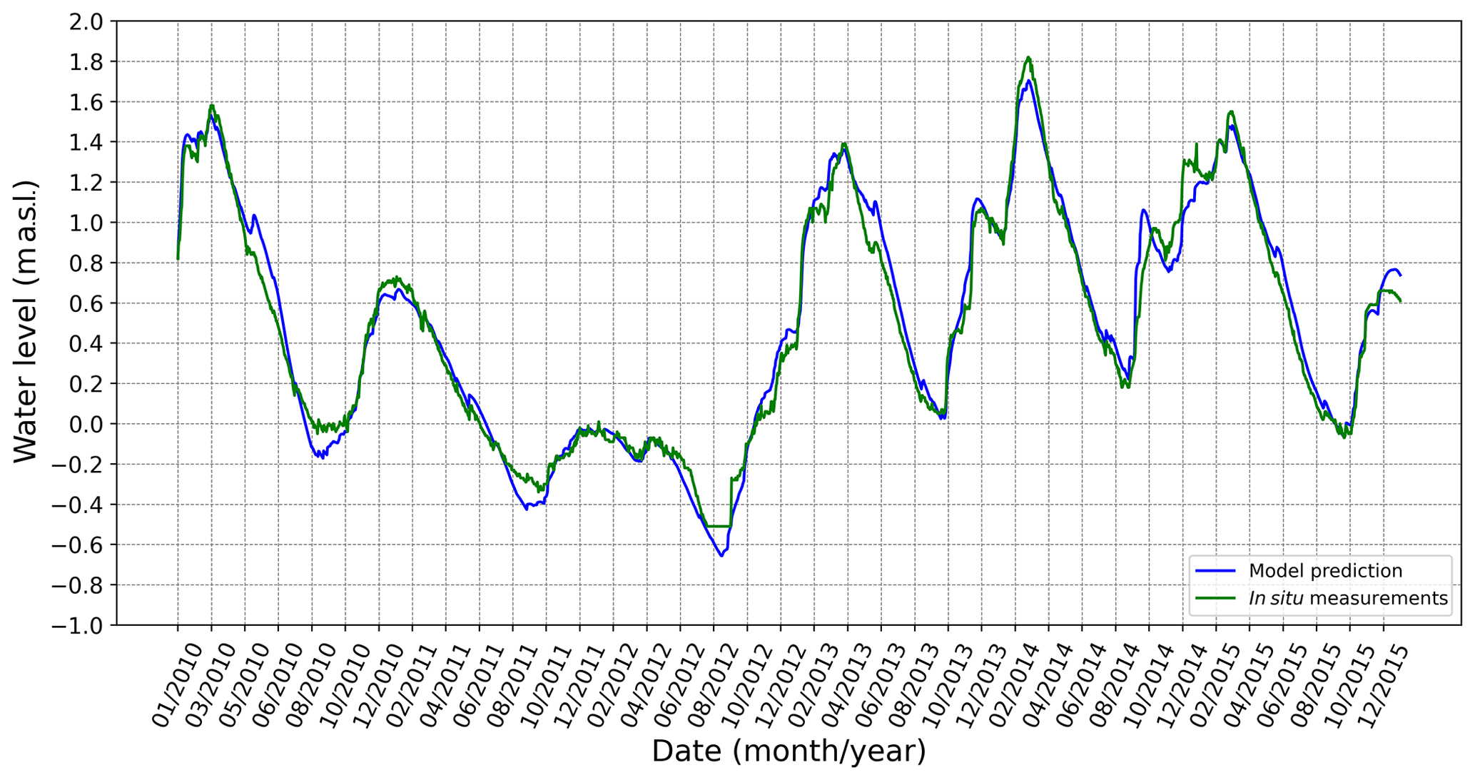
Figure 4 The predicted change in lake water level h_l(t) (blue line) obtained by the functions illustrated in Figs. 6–8 and the change in lake water level $\widehat{h}\left(t\right)$ determined by in situ measurements (green line). In the selected time domain, the drought period in August 2012 should be noted, in addition to the next three extremes that arose as a result of flood waves.

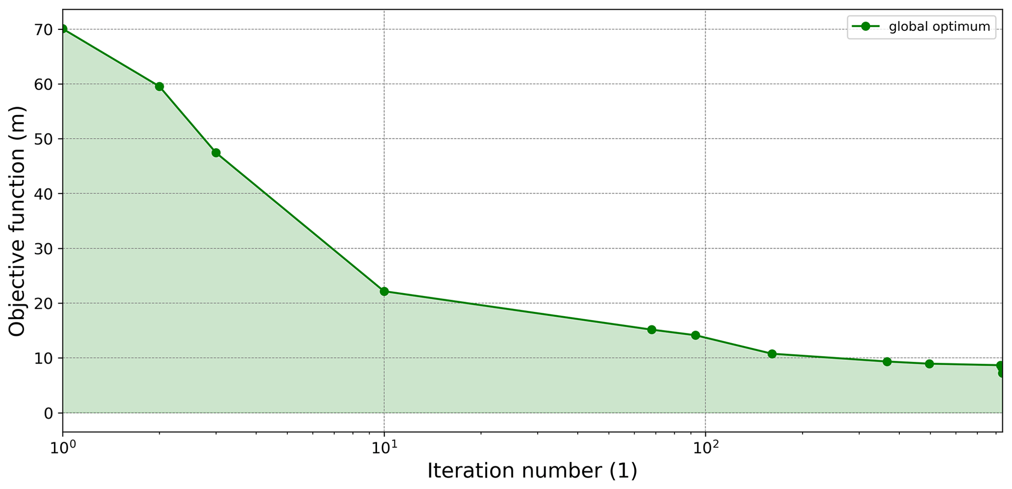
Figure 5 Global optimum points obtained for the design variables ${\mathit{x}}_{\mathrm{g},\mathrm{best}}^{\left(e\right)}$ by which the objective function reaches the so-far-established minimum.

In order to compare the presented approach with other approaches, it should be emphasized that the framework of the model is defined by a system of two ordinary and nonlinear differential equations with variable coefficients that also define the calibration functions. In these circumstances, automated methods such as genetic algorithms are usually used (Lu et al., 2018; Nematolahi et al., 2018). On the other hand, if the trial-and-error method shows that the results are very sensitive to the calibration functions (model parameters), then the application of genetic algorithms is probably not the most appropriate. This means that the sensitivity of the model results to the calibration functions indicates a large number of local minima in the objective function by which the multimodality of the problem can be recognized. In such circumstances, it is not only necessary to carry out a global search of the domain of the objective function, as carried out by the method of genetic algorithms, but it is also necessary to examine local minima in order to enable a more detailed search of the individual parts of the domain by carrying out local searches. Moreover, the search for local minima must be adaptive so that the solution in the current iteration can be updated by the new local solution that results in a more favorable variant of the calibration parameters. In this way, the possibility of searching for a larger number of local minima is realized, which is necessary for such multimodal problems. Considering all of the points mentioned, and by noting that the model in question showed the characteristics of multimodal problems, the calibration of the model was performed using the PSO method, which simultaneously performs a global and local search of the domain of the objective function (Özcan and Yilmaz, 2007; Kuok and Chiu, 2012; Zambrano-Bigiarini and Rojas, 2013). Considering the experience gained from the performed analysis, the application of the PSO method can be recommended for the calibration of semi-distributed lumped karst models based on a system of nonlinear ODEs. However, the calibration procedure should be carried out by taking into account the uncertainty in the input data of the model (as shown below).

4.1 Uncertainty in measurements and calibration functions

Since the model refers to a relatively large karst area and relies on a large database obtained by field measurements over the time span of 6 years, the model calibration procedure should be conducted by considering the uncertainty in the input data. For this purpose, it should be noted that the flow component q_kl,sf, which is related to the surface water flow into Lake Vrana, has a relatively low degree of uncertainty because it was obtained by a continuous monitoring of the surface water level in all tributaries to the lake (this requires relating the water level to the flow rate under the assumption of stationary flow conditions). Similarly, the flow component q_l,ir, related to water extraction from Lake Vrana for the irrigation of agricultural land, is also quite a reliable data source since it refers to the volume of water that is charged. On the other hand, the flow component q_l,ev, related to evaporation from the water surface of Lake Vrana, contains a certain degree of uncertainty, but this is again much smaller than the main source of uncertainty, which is related to the flow components q_l,pr and q_k,pr (i.e., precipitations on the water surface of the lake and the surrounding karst aquifer). In order to take these uncertainties into account, the error in the flow components q_l,pr and q_k,pr were modeled stochastically by a Gaussian distribution 𝒩(μ,σ) (in which μ is the mean value and σ is the related standard deviation). Accordantly, for each day i in the considered time domain, the input data of precipitation were obtained by adding the error value randomly sampled from the statistical distribution 𝒩(p_i,σ) to a known measured data p_i of precipitation (with a standard deviation σ of 5 mm d⁻¹). Therefore, the calibration of the model was carried out for a larger number of cases of precipitation (flow components q_l,pr and q_k,pr), which included the uncertainty in the precipitation data and enabled the examination of its influence on the unknown calibration functions (i.e., describing the range of potential hydraulic conductivity functions at some probability level). In other words, the calibration of the model was conducted in an iterative fashion by the repetitive application of the previously described procedure (without changing the initial parameters of the PSO method). For each generated case of precipitation, the PSO method was applied to estimate the required values of the calibration functions. In order to evaluate the estimated functions equally, for all different cases of precipitation, the application of the PSO method was carried out until the global optimum did not fall below the predefined tolerance. In this way, the calibration error in all cases was of the same order of magnitude.

In accordance with the above description, the calibration of the unknown functions was carried out for 200 cases of precipitation. In this way, for each discrete coordinate in the domain of the unknown functions, a set of 200 possible function values was estimated. In other words, the values of the calibration functions are represented with a statistical distribution for each discrete domain coordinate. In order to graphically display the schedule of obtained values, the so-called box plot diagram was used, showing the five-number summary of the obtained data set (for each point in the function domain), including the minimum, lower quartile, median (illustrated by an orange line), upper quartile, and maximum. The results of the described calibration process are shown in Figs. 6–8. For the calibration function c_kl(Δh_kl), it should be noted that, in the area of the domain from 0 to 2.5 m a.s.l., there is very little scatter around the obtained mean value (blue dots connected by a blue line), and after that, a slightly larger scatter can be recognized in the central part of the domain (Fig. 6), but again the trend of the function is well articulated (with a mean value near the middle of the interquartile range). In the case of the calibration function c_ls(Δh_ls), the deviations of the obtained values around the mean values of the hydraulic conductivity (blue dots) are almost constant (Fig. 7). In contrast to the previous hydraulic conductivity function, in this case the model predicts the exchange of water in both directions, i.e., from the lake to the sea, and vice versa. Scattering around the mean value of the function A_k(h_k) is not uniform within the domain, and the maximum uncertainty is contained in the middle of the domain, i.e., in the range from 3.0 to 5.5 m a.s.l. (Fig. 8).

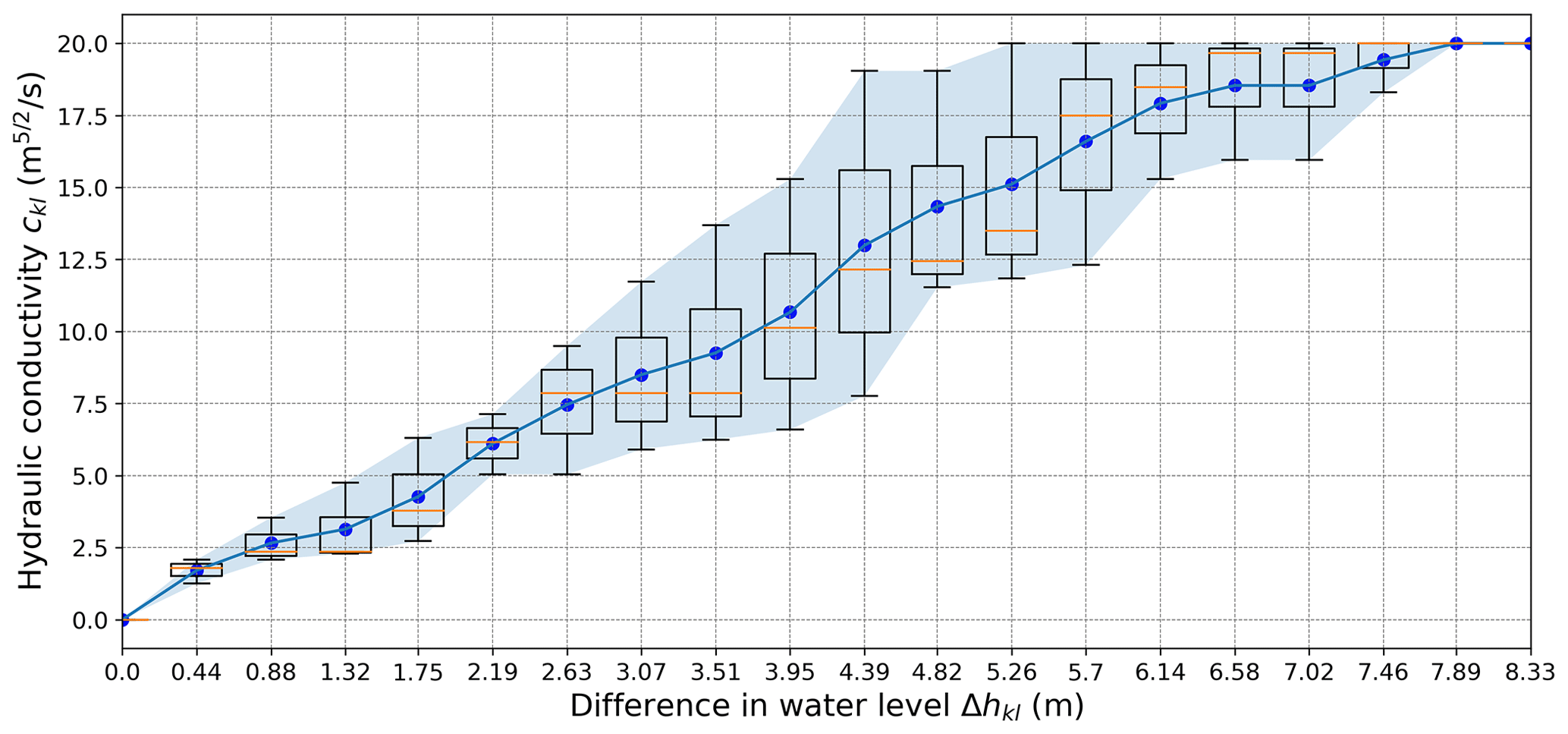
Figure 6 Statistical distribution of estimated values of the hydraulic conductivity function c_kl(Δh_kl) in Eqs. (6) and (7) required for quantifying the groundwater flow between the karst aquifer and Lake Vrana, as obtained by model calibration over a 6-year time domain (from early 2010 to late 2015), with the PSO method and adopting constraints that increase the function values by increasing the absolute values of the pressure head difference Δh_kl. It should be noted that the iterative evaluation procedure of the design function has converged into a solution that does not predict the exchange of water from the direction of Lake Vrana to the surrounding karst aquifer (which was to be expected and is recognizable in the function domain).

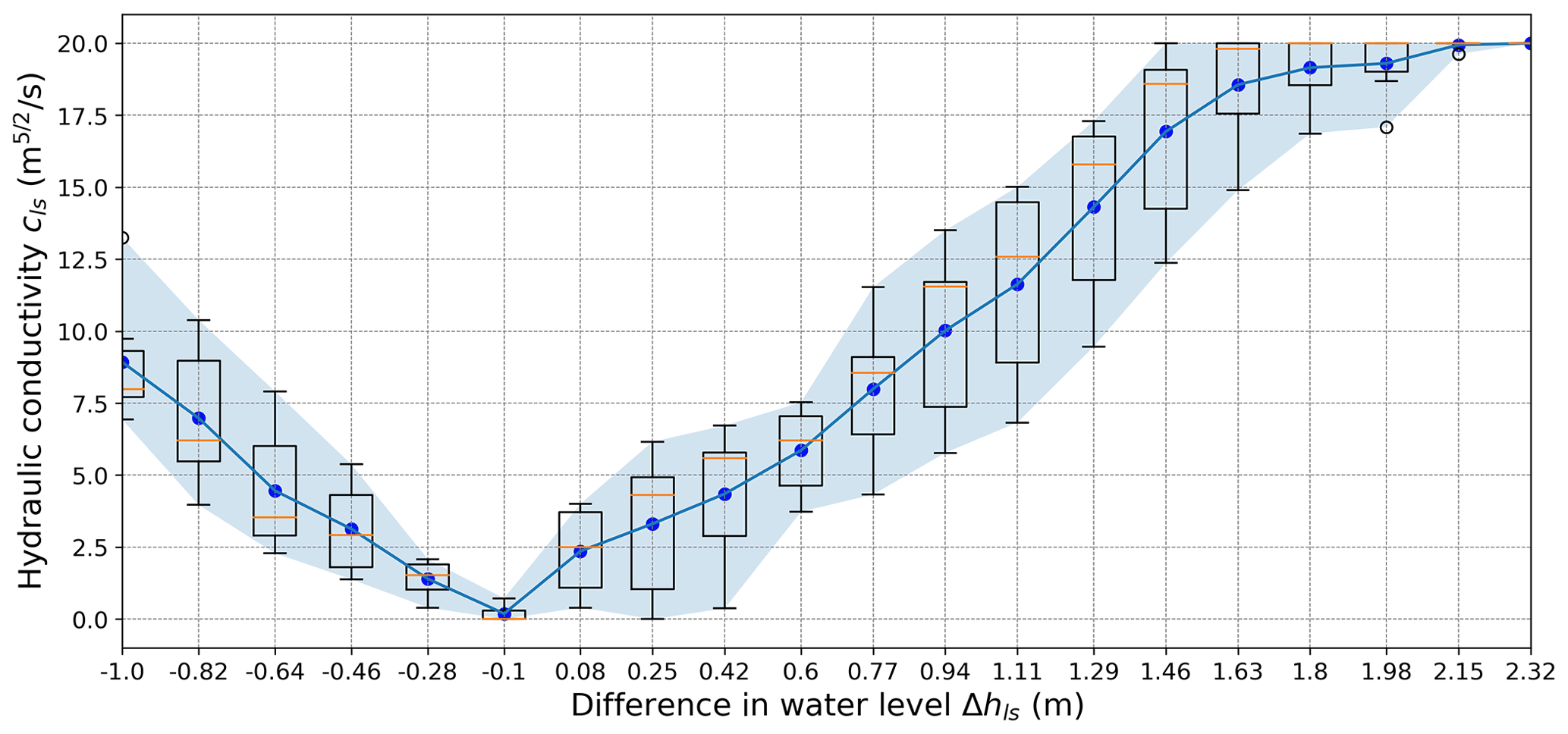
Figure 7 Statistical distribution of the estimated values of the hydraulic conductivity function c_ls(Δh_ls) in Eq. (7), which is required to quantify the groundwater flow between Lake Vrana and the Adriatic Sea, as obtained by model calibration over a 6-year time domain (from early 2010 to late 2015) by PSO method and adopting constraints that increase the function values by increasing the absolute values of the pressure head difference Δh_ls.

Figure 8 Statistical distribution of estimated values of the function A_k(h_k) in Eq. (6), as obtained by model calibration with the PSO method over a 6-year time domain (from early 2010 to late 2015), and adopting the constraint condition of a progressive reduction in the function values (i.e., requiring a negative derivation at each calibration point).

In order to reduce the uncertainty in the calibration functions, additional conditions can be included within the presented calibration procedure. In other words, the allowed ranges of the values of the calibration functions can be specified within the optimization procedure for a particular part of the domain. For this purpose, it should be noted that the most sensitive areas of the domain of calibration functions can be determined by uncertainty analysis (as in the case of Lake Vrana) and thus define the scope of additional field measurements that will provide the necessary data from which additional conditions for calibration functions can be prescribed (which will consequently reduce the uncertainty). In order to carry out the analysis of the dynamics of the exchange of fresh- and saltwater in Lake Vrana (under different protection conditions), the calibration functions shown by the blue line in Figs. 6–8 were used (defined by joining the mean values of the obtained statistical distributions).

4.2 Analysis of the existing protection against seawater intrusion

The calibrated mathematical model was used to conduct a more detailed analysis of fresh- and saltwater exchange in Lake Vrana during the considered time domain. Thus, the total volume of fresh- or saltwater that fills or empties Lake Vrana in a unit of time can be decomposed into its constituent parts given by the corresponding terms in Eqs. (5) and (6). Accordingly, Fig. 9 illustrates the origin of water volumes entering or exiting Lake Vrana, where positive volumes denote inflow quantities and negative volumes outflow quantities. It is important to recognize the volumes of water that (i) pass through Lake Vrana bed (red areas), (ii) pass through the Prosika channel bed (black areas), and (iii) overflow the weir crest at 0.41 m a.s.l. at the end of the Prosika channel (orange areas). Therefore, as the sea level in August 2011 and 2012 was above the lake water level (h_s>h_l), the model predicts the intrusion of saltwater through Lake Vrana bed and also a small contribution from the Prosika channel bed (red and black areas on the positive side). Moreover, the volume analysis can be used to estimate the amount of saltwater in Lake Vrana.

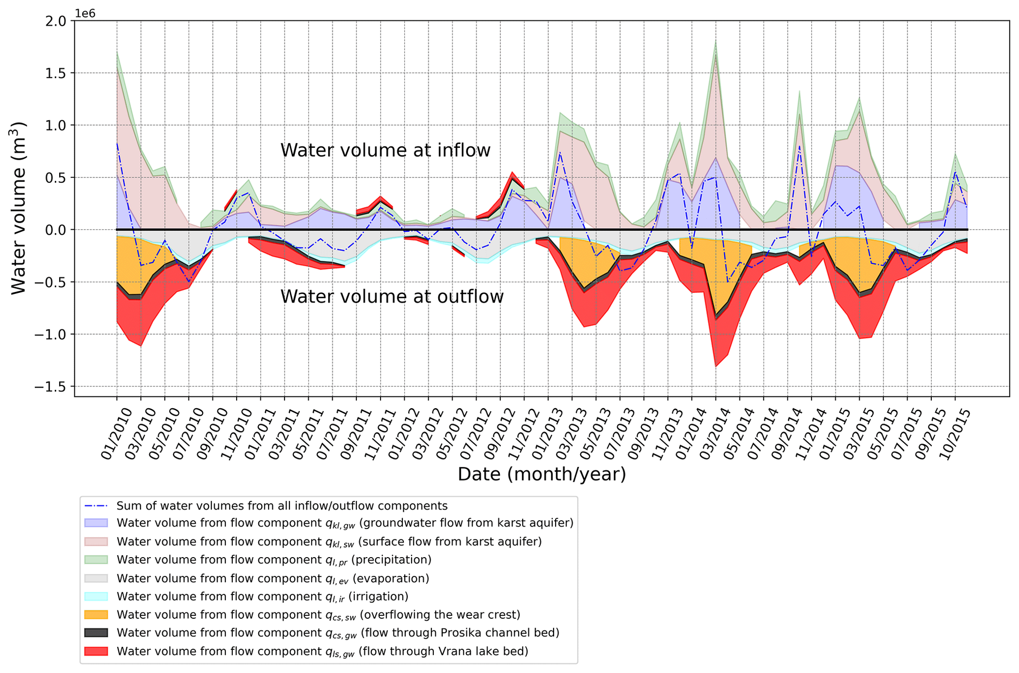
Figure 9 The decomposition of water volumes related to the inflow and outflow from Lake Vrana in the considered time domain and for the existing protection against seawater intrusion (positive values denotes volumes entering the lake and negative volumes the opposite). The intrusion of saltwater can be recognized through the Lake Vrana bed and the Prosika channel bed.

Under the assumption of only freshwater being present in Lake Vrana at the beginning of simulated time period, and the expectation that it is difficult for the contained saltwater to mix with freshwater, it is firstly squeezed out through groundwater flow if the required pressure gradient is reached (as it is denser and thus close to the lake bed), and then the volume analysis can be used to estimate the temporal change in the ratio of fresh- and saltwater in Lake Vrana, thereby giving useful information on the water quality. Accordingly, Fig. 10 illustrates the change in the ratio between fresh- and saltwater in Lake Vrana over the considered time domain. Moreover, the amount of saltwater that penetrated during the low lake water level can be monitored, in addition to the gradual extrusion of saltwater as a consequence of replenishment of freshwater in the coming period of floods.

Figure 10 The temporal change in a ratio between fresh- and saltwater in Lake Vrana in the considered time domain and for the existing protection from seawater intrusion. It should be noted that the intrusion of saltwater begins in September 2010 when, in a short time period, the lake water level falls below sea level (as shown in Fig. 3).

4.3 Analysis of the tested protection against seawater intrusion

The effectiveness of different technical solutions for protection against excessive seawater intrusion can now be tested by changing the appropriate model parameters with the intention of simulating different flow conditions. In order to illustrate the application of the model, the quantity and quality of the water in Lake Vrana (related to the lake water level and the ratio between fresh- and saltwater) was modeled by adopting a tested protection measure against seawater intrusion involving (i) the construction of a sluice gate at the end of the Prosika channel (instead of the current weir of fixed height) and (ii) lining the canal to prevent seawater intrusion through the Prosika channel bed (denoted by black areas in Fig. 9). Thus, a sluice gate is necessary in order to preserve the possibility of evacuating a large amount of water during the flooding period. At the same time, the sluice gate can be used to prevent water overflow (denoted by orange areas in Fig. 9), thereby achieving the retention of freshwater in the lake.

Figure 11 Comparison of the measured lake water level (blue line) for the existing protection from seawater intrusion and the lake water level obtained for the tested protection from seawater intrusion (red line), which includes (i) the sluice gate at the end of the Prosika channel and (ii) lining the Prosika channel bed.

To illustrate the benefit of the introduced sluice gate, it was necessary to define an algorithm for its movement during dry and wet periods. For this purpose, the gate movement was defined as a function of the current lake water level h_l(t). In order to contribute to the retention of freshwater during the dry period, the gate crest in the lowered position was set at 1.05 m a.s.l., preventing the overflow of freshwater and saltwater intrusion by surface flow in the Prosika channel (term q_cs,sw). During flood periods, the gate is raised so that the overflowing crest level is at 0.15 m a.s.l., i.e., at the Prosika channel bottom (thus achieving maximum throughput).

Figure 12 The decomposition of the water volumes related to inflow and outflow from Lake Vrana in the considered time domain and for a hypothetical protection variant involving lining the Prosika channel bed and raising the level of the downstream overflow.

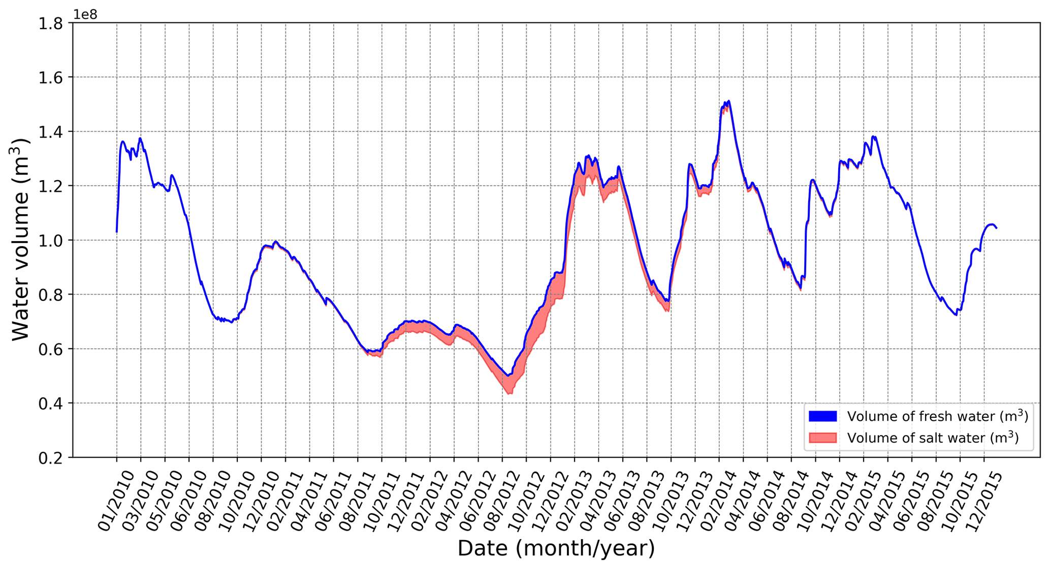
Figure 13 The temporal change in the ratio between fresh- and saltwater in Lake Vrana in the considered time domain and for a tested protection measure involving a sluice gate at the end of the Prosika channel and lining the Prosika channel bed.

For the described gate-control algorithm, Fig. 11 shows the achieved lake water level variation in the considered time domain and under the same hydrological conditions as used previously. By comparing the obtained time change in the lake water level (red line) with the one measured for the existing state of protection against seawater intrusion (blue line), it should be noted that the lake water level increases negligibly during the dry period in August 2012. However, the effectiveness of the considered protection can be recognized by performing the decomposition of water volumes entering or leaving Lake Vrana per unit of time (as in the previous case). Accordingly, Fig. 12 shows the decomposition of the water volumes obtained for the tested protection case. The lining of the channel bed excluded the component of water exchange that takes place through the porous Prosika channel bed (denoted by black areas in Fig. 9), as obtained for the existing protection case. Notwithstanding, it should be noted that the presence of a gate increased the flow through the Lake Vrana bed (denoted by red regions in Fig. 12). This result should not be surprising because the gate activity raises the lake water level most of the time (as shown in Fig. 11) and consequently raises the pressure gradient and in turn the component of sinking flow described by the term q_ls,gw. The benefit of the tested protection measure case can be recognized if the temporal change in the ratio of fresh- and saltwater is observed (as done previously). Although the flow of water from the lake is higher (resulting from rising water levels in the lake), the total amount of saltwater in the lake decreases as a consequence of lining the Prosika channel bed (preventing one component of seawater intrusion) and also retaining a larger amount of freshwater in the lake. The resulting benefit can be recognized by comparing Figs. 10 and 13. Finally, it should also be noted that the gate presence with the given maneuvering algorithm did not disrupt the flood protection, as the maximal lake water level did not increase.

5 Conclusions

The application of a semi-distributed lumped karst model requires the estimation of hydraulic conductivity functions by which the relationship between the difference in the pressure head along karst conduits (related to the pressure gradient) and the achieved groundwater flow is described. An iterative method, based on the application of PSO method, has been proposed for the estimation of these functions. Accordingly, the inverse modeling task is considered to be an optimization problem which is carried out by minimizing the objective function through which the difference between the predicted hydrological quantity and the measured one (e.g., water level under the same hydrological conditions) is quantified. For this purpose, it was necessary to provide all relevant hydrological and other data in a representative time domain that includes hydrological extremes. For illustrative purposes, the proposed procedure was applied to model the exchange of fresh- and saltwater in Lake Vrana in Croatia. To estimate the hydraulic conductivity functions related to groundwater flow between Lake Vrana and the surrounding karst aquifer and the Adriatic Sea, a time domain that spans over 6 years was considered. Apart from the unknown hydraulic conductivity functions, the functions that relate groundwater level in a karst aquifer to the corresponding horizontal cross-area of karst conduits were also estimated by the procedure. To reduce the number of all possible solutions, additional constraint conditions were applied to the unknown functions. Within a reasonable number of evaluation steps, the procedure converged to a solution by which the computed time change in the lake water level was approximately equal to the measured lake water level over the entire time domain (including dry and wet periods).

The calibrated model was used to analyze the current protection of Lake Vrana from saltwater intrusion. For this purpose, a decomposition of the total water volume inside Lake Vrana was conducted, based on the origin of the water and the direction of the flow (inflow or outflow). By assuming no saltwater at the beginning of the time domain, the conducted analysis was used to monitor the volume ratio of fresh- and saltwater in the lake. To increase the quality and also the quantity of water in Lake Vrana, an alternative measure to protect against saltwater intrusion was tested. The considered protection case included (i) lining the Prosika channel bed and (ii) constructing a sluice gate at the end of Prosika channel. For the same hydrological conditions and time domain, the tested protection solution did not prevent the lake water level from falling to the lowest point (as compared to the existing protection system). However, the decomposition of the water volume that enters and exits the lake revealed a smaller amount of saltwater compared to the existing protection system.