Soil moisture estimates at 1 km resolution making a synergistic use of Sentinel data

Very high-resolution (∼10–100 m) surface soil moisture (SM) observations are important for applications in agriculture, among other purposes. This is the original goal of the S²MP (Sentinel-1/Sentinel-2-Derived Soil Moisture Product) algorithm, which was designed to retrieve surface SM at the agricultural plot scale by simultaneously using Sentinel-1 (S1) backscatter coefficients and Sentinel-2 (S2) NDVI (Normalized Difference Vegetation Index) as inputs to a neural network trained with Water Cloud Model simulations. However, for many applications, including hydrology and climate impact assessment at regional level, large maps with a high resolution (HR) of around 1 km are already a significant improvement with respect to most of the publicly available SM datasets, which have resolutions of about 25 km.

In this study, the S²MP algorithm was adapted to work at 1 km resolution and extended from croplands to herbaceous vegetation types. A target resolution of 1 km also allows the evaluation of the interest in using NDVI derived from Sentinel-3 (S3) instead of S2. Two sets of SM maps at 1 km resolution were produced with S²MP over six regions of ∼10⁴ km² in Spain, Tunisia, North America, Australia, and the southwest and southeast regions of France for the whole year of 2019. The first set was derived from the combination of S1 and S2 data (S1 + S2 maps), while the second one was derived from the combination of S1 and S3 (S1 + S3 maps). S1 + S2 and S1 + S3 SM maps were compared to each other, to those of the 1 km resolution Copernicus Global Land Service (CGLS) SM and Soil Water Index (SWI) datasets, and to those of the Soil Moisture Active Passive (SMAP) + S1 product.

The S²MP S1 + S2 and S1 + S3 SM maps are in very good agreement in terms of correlation (R≥0.9), bias (≤0.04 m³ m⁻³), and standard deviation of the difference (SDD≤0.03 m³ m⁻³) over the six domains investigated in this study. In a second step, the S1 + S3 S²MP maps were compared to the other HR maps. S1 + S3 SM maps are well correlated to the CGLS SM maps (R∼0.7–0.8), but the correlations with respect to the other HR maps (CGLS SWI and SMAP + S1) drop significantly over many areas of the six domains investigated in this study. The highest correlations between the HR maps were found over croplands and when the 1 km pixels have a very homogeneous land cover. The bias among the different maps was found to be significant over some areas of the six domains, reaching values of ±0.1 m³ m⁻³. The S1 + S3 maps show a lower SDD with respect to CGLS maps (≤0.06 m³ m⁻³) than with respect to the SMAP + S1 maps (≤0.1 m³ m⁻³) for all the six domains.

Finally, all the HR datasets (S1 + S2, S1 + S3, CGLS, and SMAP + S1) were also compared to in situ measurements from five networks across five countries, along with coarse-resolution (CR) SM products from SMAP, SMOS, and the European Space Agency Climate Change Initiative (CCI). While all the CR and HR products show different bias and SDD, the HR products show lower correlations than the CR ones with respect to in situ measurements. The discrepancies in between the different HR datasets, except for the more simple land cover conditions (homogeneous pixels with croplands) and the lower performances with respect to in situ measurement than coarse-resolution datasets, show the remaining challenges for large-scale HR SM mapping.

1 Introduction

Surface soil moisture (SM) plays a key role in the Earth water cycle as it affects many hydrological processes such as infiltration, runoff, evaporation, and precipitation (Koster et al., 2004). SM measurements are used to constrain numerical weather prediction (NWP) models via data assimilation (De Rosnay et al., 2013; de Rosnay et al., 2014; Rodríguez-Fernández et al., 2019) in addition to crop yield forecasting, food security, and agriculture management (Guerif and Duke, 2000). SM was identified as one of the 50 essential climate variables (ECVs) by the Global Climate Observing System in the context of the United Nations Framework Convention on Climate Change (Plummer et al., 2017; GCOS, 2021). Building long time series of SM is crucial for climate applications, and this is the goal of projects such as the European Space Agency's Climate Change Initiative (ESA CCI) for SM (Gruber et al., 2019).

Both active and passive microwave sensors can be used to estimate SM at coarse resolutions (∼25–40 km), including the active Advanced SCATterometer (ASCAT; Vreugdenhil et al., 2016), the passive Advanced Microwave Scanning Radiometer 2 (AMSR2; Kim et al., 2015; Imaoka et al., 2000), and the two sensors that have been specifically designed to measure SM at L band, namely the Soil Moisture and Ocean Salinity (SMOS; Kerr et al., 2012) and Soil Moisture Active Passive (SMAP; Entekhabi et al., 2010). However, despite the actual availability of these SM products, they do not match the requirements of a number of applications. Peng et al. (2020) have discussed a roadmap and the requirements for future SM products. An optimal spatial resolution for data assimilation into NWP models and reanalysis would be 5–10 km (global models are already running with resolutions better than 10 km; see, for instance, Muñoz-Sabater et al., 2021). The evaluation of climate models and the assessment of climate change impacts at a regional level would also benefit from a higher resolution than that of the current generation of coarse-resolution sensors. In addition, other applications in hydrology, agriculture, and risk assessment require even higher resolutions of ∼1 km (Massari et al., 2021).

Downscaling the coarse-scale-resolution data by merging them with higher-resolution data is a possibility for the achievement of high-resolution SM datasets. For example, high-resolution SM estimates can be derived from visible/infrared (Merlin et al., 2012) or synthetic-aperture radar (SAR; Tomer et al., 2016; Das et al., 2019) measurements. SAR observations alone have also been tested to estimate SM using different frequencies and instruments such as RADARSAT, ALOS-L, or TerraSAR-X. Radar signal is not only sensitive to the dielectric constant linked to SM but also to surface geometry (including roughness) and vegetation water content and structure (Ulaby et al., 1986). Different inversion algorithms have been proposed, considering principally three techniques, i.e., change detection algorithms (Wagner et al., 1999; Balenzano et al., 2010; Bauer-Marschallinger et al., 2018), direct inversion of physical or empirical models (Moran et al., 2000; Srivastava et al., 2009; Pierdicca et al., 2010; Hajj et al., 2014; Bousbih et al., 2017; Şekertekin et al., 2018), and machine learning methods (Paloscia et al., 2004; Notarnicola et al., 2008; El Hajj et al., 2017).

With the successive launches of the C-band SARs on board Sentinel-1A (S1A, 2014) and Sentinel-1B (S1B, 2016), SM can be estimated at high spatial resolution and with a revisit time of better than 6 d over Europe. Three operational high-resolution (HR) SM datasets at 1 km resolution using Sentinel-1 (S1) exist, such as the S1 SM and Soil Water Index (SWI) products from the Copernicus Global Land Service (CGLS; Bauer-Marschallinger et al., 2018, 2019) and the SMAP + S1 downscaled product (Das et al., 2020). SM estimates at a very high resolution (10 m scale) at some locations in Europe (and in Lebanon and Morocco) over croplands are also distributed by the French continental surfaces data center (THEIA; https://www.theia-land.fr, last access: November 2021). In contrast to the CGLS datasets, the THEIA SM dataset is obtained using synergistic S1 and Sentinel-2 (S2) measurements as inputs to the Sentinel-1/Sentinel-2-Derived Soil Moisture Product (S²MP) algorithm (El Hajj et al., 2017). This dataset has been evaluated against in situ measurements in comparison to SMAP, SMOS, and ASCAT coarse-resolution (CR) datasets (El Hajj et al., 2018) and with respect to the CGLS S1 SM dataset (Bazzi et al., 2019), both in the south of France. The S²MP SM estimates not only showed the lowest unbiased root mean squared errors with respect to in situ measurements but also a moderate correlation, lower than that obtained for SMAP and ASCAT datasets (El Hajj et al., 2018). In this region, the S²MP SM showed better performances with respect to in situ measurements than the CGLS SM for the classical metrics (Bazzi et al., 2019).

Taking into account the importance of having accurate HR large-scale SM datasets, in this study the S²MP algorithm was extended to provide SM estimates over both croplands and herbaceous vegetation at 1 km resolution, which also allowed the use of the Sentinel-3 (S3) NDVI (Normalized Difference Vegetation Index) instead of S2.

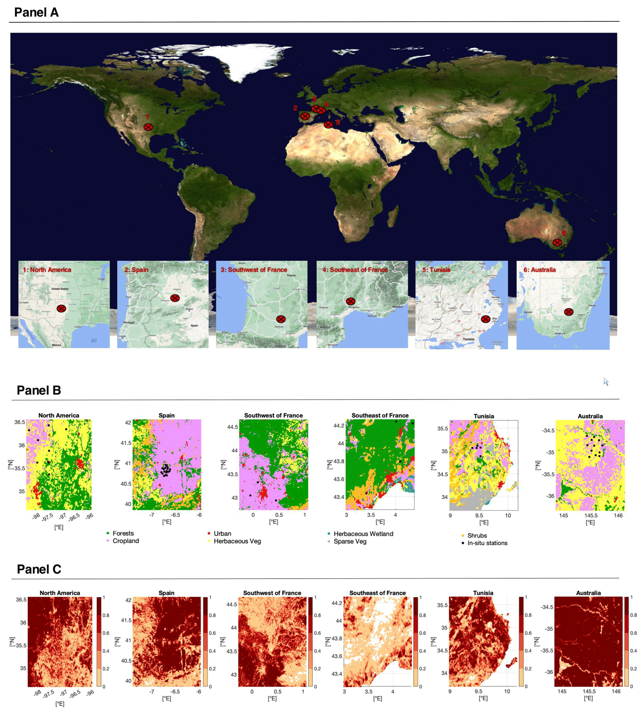
Figure 1 (a) Global locations of the six regions of study (© Google Maps 2022). (b) Copernicus land cover maps of the six regions of study aggregated at 1 km spatial resolution. Only the dominant land cover type within a 1 km² pixel is shown. For instance, a pixel characterized as forests can contain 27 % of forests, 26 % of croplands, 24 % of herbaceous vegetation, and 23 % of shrublands or 90 % of forests and 10 % of herbaceous vegetation. The in situ stations are shown as black dots. One black dot can correspond to several sensors, since some of them have the same coordinates. (c) Proportion of croplands and herbaceous vegetation within each 1 km² pixel for the six regions of study. The proportion is expressed as a percentage ranging from 0 to 1. Pixels with no cropland or herbaceous vegetation at all are shown as white areas.

Two sets of SM maps at 1 km resolution were produced with the S²MP algorithm over six domains of ∼10⁴ km² in Tunisia, North America, Spain, Australia, and the southwest and southeast of France (Fig. 1a). One set is based on the combination of S1 and S2 measurements (S1 + S2 maps), while the other is based on the combination of S1 and S3 measurements (S1 + S3 maps). The S²MP S1 + S2 and S1 + S3 maps were compared to those provided by the SMAP + S1 product and those from the CGLS SM and SWI datasets from January to December 2019. The comparison was carried out on a per-pixel basis, and the results were analyzed according to pixel homogeneity for areas covered by croplands and herbaceous vegetation. In addition, the HR time series were evaluated against in situ measurements along with those of the coarser-resolution SM datasets from SMAP, SMOS, and ESA CCI.

The paper is structured as follows. Section 2 presents the different remotely sensed and ground-based data that are used in this study. Section 3 describes the methodology used to estimate SM over croplands and herbaceous regions using S1 + S3. Section 4 shows the S1 + S3 S²MP maps and time series. They are also compared to the S1 + S2 maps in addition to other HR datasets, coarse-resolution datasets, and in situ measurements. Section 5 discusses the interest of the S²MP algorithm modifications and the remaining challenges for large-scale HR SM mapping. Section 6 draws the conclusions of the study.

2 Data

2.1 Soil moisture maps computation

2.1.1 Sentinel-1

The Sentinel-1 mission is the first satellite constellation mission of the Copernicus program and was conducted by ESA. The mission is composed of a constellation of two satellites sharing the same orbital plane. S1A was launched on 3 April 2014 and S1B on 25 April 2016. They were placed in a near-polar, sun-synchronous orbit. The revisit frequency is 12 d over Europe (6 d using both satellites), with an Equator-crossing time at 18:00 LT (local time) for the descending overpass. S1A and S1B carry a C-band (wavelength ∼6 cm) SAR imaging instrument on board, enabling the acquisition of imagery regardless of the weather and the time of the day.

For the production of the S²MP SM maps, S1A and S1B SAR images were collected over each region of study. S1 images are accessible from the Copernicus Open Access Hub. The S1 images (10 m × 10 m) were acquired in the interferometric wide (IW) swath imagining mode, with VV (vertical transmit, vertical receive) and VH (vertical transmit, horizontal receive) polarizations, and the S1 Toolbox (S1TBX) developed by the ESA was used to calibrate the images. This calibration aims to convert digital number values from S1 images into backscattering coefficients (${\mathit{\sigma }}^{{}^{\circ }}$) in a linear unit and orthorectifying the images using the Shuttle Radar Topography Mission (SRTM) digital elevation model (DEM) at 30 m spatial resolution. A database of S1 images, available from January to December 2019, was created for each region of study. The databases contain S1 images acquired both in ascending (afternoon) and descending (morning) modes.

2.1.2 Sentinel-2

The Sentinel-2A and 2B (S2A and S2B) satellites were launched on 23 June 2015 and 7 March 2017 and were placed in a near-polar, sun-synchronous orbit. The revisit frequency is 10 d (5 d with two satellites), and the descending orbit crossing time at Equator is 10:30. The spatial coverage ranges from 56^∘ S to 84^∘ N. The satellites carry a multispectral instrument with 13 bands on board, with four bands at 10 m, six bands at 20 m, and three bands at 60 m spatial resolution. The orbital swath width is 290 km (Spoto et al., 2012).

For the production of the S²MP SM maps based on S1 and S2, optical images from S2A on dates close to S1 SAR images (less than 2 weeks) were downloaded from the French land data service center (THEIA) website (https://www.theia-land.fr/, last access: November 2021). The S2A optical images (10 m × 10 m) are corrected for atmospheric effects and orthorectified.

2.1.3 Sentinel-3

The Sentinel-3A and 3B (S3A and S3B) satellites were launched on 16 February 2016 and on 25 April 2018, respectively. The S3 satellites' orbit is a near-polar, sun-synchronous orbit with an Equator-crossing time of 10:00 LT for the descending overpass. They carry an optical instrument payload on board (the Ocean and Land Colour Instrument, OLCI) that samples 21 spectral bands ([0.4–1.02] µm) with a swath width of 1270 km and a spatial resolution of 300 m. They also carry a dual-view scanning temperature radiometer at 500 m spatial resolution, i.e., the Sea and Land Surface Temperature Radiometer (SLSTR). The revisit frequency of these instruments is 2 d when both satellites are used together (Donlon et al., 2012).

In this study, the S3 10 d synthesis NDVI at 1 km spatial resolution was used for the production of the S²MP SM maps based on S1 and S3. These data are accessible from the SY_2_V10 product (Henocq et al., 2018) and were downloaded from the Copernicus Open Access Hub. The data from this product rely upon the synergistic use of the OLCI and SLSTR instruments. The product provides a 1 km VEGETATION-like product, including 10 d synthesis surface reflectances and NDVI. The NDVI values correspond to a maximum NDVI value composite of all segments received for 10 d.

2.2 Data used for evaluation

2.2.1 Copernicus Global Land Service

Two Copernicus Global Land Service (CGLS) datasets were used to compare with the S²MP maps.

• i.

  The CGLS V111 S1 Surface Soil Moisture product (hereafter CoperSSM) is retrieved from the S1 radar backscatter images over the European continent at 1 km resolution (Bauer-Marschallinger et al., 2019). The images are acquired at C-band SAR in VV polarization, and the retrieval approach is based on a change detection algorithm (Bauer-Marschallinger et al., 2018). Changes observed in the C-band SAR backscatter coefficient are interpreted as changes in the SM values, whereas other surface properties such as the geometry, surface roughness, and vegetation cover are assumed to be static in time for each pixel. The algorithm provides local relative SM values in percentages ranging between 0 % and 100 %, except in the case of extremely dry conditions, frozen soil, snow-covered soil, and flooding. The data are sampled at 1 km resolution from 11^∘ W to 50^∘ E and from 35 to 72^∘ N.

• ii.

  The CGLS V101 S1 Soil Water Index product (hereafter CoperSWI) is derived from a fusion of surface SM observations from S1 C-band SAR and Metop ASCAT sensors (Bauer-Marschallinger et al., 2018). It uses a two-layered water balance model that is adapted to use a recursive formulation and does not account for soil texture. A Surface State Flag (SSF) that indicates the frozen, unfrozen, and/or melting state of the surface, depending on the temperature, is used to identify SM values under non-frozen conditions to be used for the SWI calculation. SWI and quality flag values are calculated based on a phenomenological formulation that depends on the characteristic time length parameter (hereafter T). A large T value represents an increase in reservoir depth or a decreased pseudo-diffusivity coefficient. This means that, for a fixed pseudo-diffusivity constant, an increased T value represents a deeper soil layer (Paulik et al., 2014). SWI estimations for eight different T values are provided within the product. Previous evaluations of SWI data by Paulik et al. (2014) and Albergel et al. (2008) showed that the best agreement with in situ measured surface SM is usually obtained with T values in the range of 5–10; therefore, SWI data with T=5 were used in this study.

2.2.2 SMAP products

SMAP provides passive measurements of 1.4 GHz brightness temperatures in vertical and horizontal polarizations at a fixed incidence angle of 40^∘, with a resolution of ∼45 km (Entekhabi et al., 2014). SMAP ascending and descending orbits cross the Equator at 18:00 and 06:00 LT, respectively, and the maximum revisit period is 3 d. Several HR and CR SM datasets from SMAP were used for the evaluation of the S²MP maps.

• i.

  The SMAP L3 V6 SM product (hereafter SMAPL3). It is a daily gridded composite of the SMAP L2 V5 SM files (O'Neill et al., 2018, 2019b). Only SM estimates derived from L1C brightness temperatures (Chan et al., 2018) using the single-channel algorithm V-polarization (Entekhabi et al., 2010) were considered. SMAP L3 data are sampled at 36 km resolution.

• ii.

  The SMAP Enhanced L3 V1 SM product (hereafter SMAPL3E), which is obtained by oversampling the L1C brightness temperatures from 36 to 9 km resolution using an interpolation algorithm (O'Neill et al., 2019a). Only SM estimates derived using the single-channel algorithm V-polarization were considered.

• iii.

  The SMAP + S1 L2 V1 SM product (hereafter SMAPS1) provides SMs at 1 km resolution that are estimated using the SMAP enhanced L3 V004 half-orbit at 9 km resolution and Copernicus S1A and S1B C-band SAR data (Das et al., 2020). Brightness temperatures from SMAP are disaggregated on the 1 km Equal-Area Scalable Earth (EASE) Grid by using the S1 radar backscatter data, and HR SM estimates are obtained using the SMAP algorithm. The closest data in time between descending and ascending orbits from SMAP are used to spatially match up with the S1 scene.

2.2.3 SMOS

The SMOS mission (Kerr et al., 2010) carries a passive interferometric radiometer operating at the L band (21 cm, 1.4 GHz), with a spatial resolution of 25–50, depending on the position on the field of view (43 km on average). The following CR SM datasets from SMOS were used in this study:

• i.

  The CATDS SMOS L3 V7 SM product (hereafter SMOSL3), which is a multi-orbit SM product, provided by the Centre Aval de Traitement des Données (CATDS), with a grid resolution of 25 km (Al Bitar et al., 2017). The SM retrieval process is based on the algorithm used for the SMOS L2 product (Kerr et al., 2012) but simultaneously using three orbits within a 1-week period to better constrain the SM and optical depth estimations.

• ii.

  The ESA SMOS Near-Real Time (NRT) Neural Network (NN) V2 SM product (hereafter SMOSNRT), provided on the icosahedral equal area grid (ISEA4H9), with 15 km resolution (Rodríguez-Fernández et al., 2017). It is designed to provide SM in less than 3.5 h after sensing. The algorithm uses a NN-trained sequence using SMOS L2 SM data (Kerr et al., 2012). The input data for the NN are SMOS brightness temperatures, with incidence angles from 30 to 45^∘ for horizontal and vertical polarizations, and soil temperature in the 0–7 cm layer from the European Centre for Medium-Range Weather Forecasts (ECMWF) models.

Gonzalez-Zamora et al. (2018)Calvet et al. (2007)Calvet et al. (2007)Smith et al. (2012); Young et al. (2008)Bell et al. (2013)Cook (2016, 2018)Amri et al. (2011)Gorrab et al. (2015)

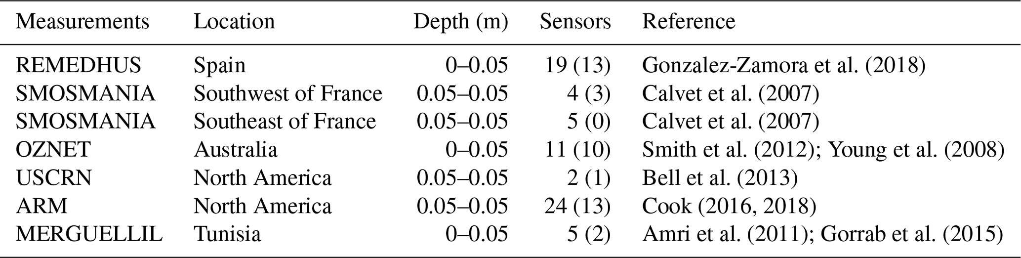
Table 1 In situ measurements that were used in this study. The depths are given as two numbers, where the first one is the upper depth of the sensor, and the second one is the lower depth of the sensor. Both numbers are equal when the sensor is placed horizontally. The fourth column shows the number of sensors that provide SM measurements in 2019. These measurements were used to convert the relative indices from CoperSSM and CoperSWI into SM estimates with volumetric units (m³ m⁻³; Sect. 3.2). The number in parenthesis corresponds to the number of in situ locations where the evaluations of the remotely sensed data were significant (P value below 5 %; Sect. 3.3).

2.2.4 ESA CCI COMBINED product

In the COMBINED product of ESA SM CCI V5.2 (hereafter CCISM; Dorigo et al., 2017; Gruber et al., 2019), L2 datasets from different active and passive sensors are directly scaled by matching their cumulative density functions (CDFs) to that of the Global Land Data Assimilation System (GLDAS; Rodell et al., 2004) Noah land surface model in order to remove relative biases and harmonize their dynamical ranges. In the period of this study, ESA CCI COMBINED uses the H SAF active sensor products from the Advanced SCATterometer A and B (ASCAT; Wagner et al., 2013) and the passive sensor products from the Advanced Microwave Scanning Radiometer 2 (AMSR2; Kim et al., 2015; Imaoka et al., 2000), in addition to those from SMAP and SMOS. SM data from the passive sensors are estimated using the land parameter retrieval model (LPRM) V6 (Van der Schalie et al., 2016, 2017). The data are sampled at 25 km resolution.

2.2.5 Land cover

The Copernicus Global Land Service (CGLS) V3 Dynamic Land Cover map product delivers a global land cover map at 100 m resolution, covering the period between 2015 to 2019 (Buchhorn et al., 2020). For each year, a land cover map is provided with three different levels of classes, including 11 classes at level 1 (all types of forests are considered to be a unique land cover class), 13 classes at level 2 (forests are split in two land cover classes of open and closed forests), and up to 22 classes at level 3 (all types of open and closed forests are considered). In this study, only the 2019 land cover map at level 1 was considered. Figure 1b shows the seven land cover classes that are represented in the six regions of study. In this figure, the land cover map was aggregated from 100 m to 1 km resolution for evaluation purposes, meaning that only the dominant land cover for each 1 km² pixel is shown.

2.2.6 In situ measurements

The evaluation against in situ measurements of soil moisture was performed using data from the REMEDHUS (Gonzalez-Zamora et al., 2018), SMOSMANIA (Calvet et al., 2007), OZNET (Smith et al., 2012; Young et al., 2008), USCRN (Bell et al., 2013), ARM (Cook, 2016, 2018), and the MERGUELLIL networks (Amri et al., 2011; Gorrab et al., 2015) that are located within the six regions of this study (Table 1). All data, except those from the MERGUELLIL network, were retrieved from the International Soil Moisture Network (ISMN; Dorigo et al., 2011, 2021). Only sensors between 0 and 5 cm depth were considered. In total, 65 ISMN and 5 MERGUELLIL sites were used for the scaling of the CoperSSM and CoperSWI data (Sect. 3.2). Fewer sites (40 from ISMN and 2 from MERGUELLIL) were used to assess the remotely sensed data, following the criteria explained in Sect. 3.3. The different in situ stations can be located using Fig. 1a and b.

3 Methods

3.1 Building S²MP maps using NDVI derived from Sentinel-3

The S²MP algorithm (El Hajj et al., 2017) was originally designed to estimate surface SM at the scale of agricultural plots (10 m resolution) using synergistically data derived from the S1 radar signal and the S2 optical images as input to a neural network. The neural network was first trained using a synthetic database gathering (i) SAR C-band backscatter coefficients in the VV polarization, (ii) incidence angles (from 20 to 45^∘), and (iii) NDVI as input and SM examples as a target. This synthetic database was built using a Water Cloud Model (Baghdadi et al., 2017) combined with an Integral Equation Model (Baghdadi et al., 2006, 2011) that was specially modified and optimized for this application. Then, the S²MP algorithm was applied to a real database gathering the SAR backscatter coefficient in VV polarization from S1, the incidence angle of the SAR acquisitions, and the NDVI derived from optical images taken by S2 as follows. First, the NDVI was computed at 10 m spatial resolution (native resolution of S2) using the atmospherically and orthorectified S2 images. To overcome the cloud cover issue present in optical images, a gap-filling procedure was performed using the linear interpolation to obtain two cloud-free NDVI images per month (1st and 15th of each month). To derive S2 NDVI data at the S1 acquisition dates, a linear interpolation was performed for each S2 pixel, using the NDVI values corresponding to the closest S2 images acquired before and after the S1 date. Second, the 10 m resolution S1 backscattering signal, incidence angle, and S2 NDVI were averaged for each 100 m pixel from the CGLS land cover map. Then, the SM estimation using the S²MP algorithm was performed at 100 m spatial resolution over pixels covered by croplands, using the CGLS land cover map described above (see Sect. 2.2.1). There is no retrieval for other types of land cover.

In contrast to the (El Hajj et al., 2017) approach described above, in the current study, S1 + S2 maps were also computed for 100 m pixels covered by herbaceous vegetation. In addition, the 100 m SM estimations were aggregated to 1 km. On the other hand, HR SM maps were also produced using NDVI from the SY_2_V10 product at 1 km resolution from S3 (see Sect. 2.1.3). Due to the spatial resolution of the S3 NDVI, the S1 backscattering signal and incidence angle were first aggregated from 10 to 100 m resolution and then re-aggregated from 100 m to 1 km but only over croplands and herbaceous vegetation. Then, the neural network was only applied over the 1 km² pixels that are partly or entirely covered by croplands and/or herbaceous vegetation. The objective was to assess the impact of using a lower spatial resolution NDVI as input to the S²MP algorithm.

Hereafter, S²MP_S1S2 and S²MP_S1S3 will refer to the S²MP SM datasets derived based on the synergistic use of S1 + S2, and S1 + S3 measurements, respectively. S²MP_S1S2 and S²MP_S1S3 were produced from January to December 2019.

For both S²MP_S1S2 and S²MP_S1S3, it is important to highlight again that there is no SM estimate available over 1 km² pixels not covered at all by croplands and herbaceous vegetation. However, as long as there is a fraction of croplands and/or herbaceous vegetation (whatever the amount) within the pixel, SM values are provided. The proportion of croplands and herbaceous vegetation within each 1 km² pixel for the six regions of study is shown in Fig. 1c.

3.2 CoperSSM and CoperSWI rescaling

Relative SM indices from CoperSSM and CoperSWI were scaled against in situ measurements for each region independently. This process is needed to transform the indices into SM estimates with volumetric units (m³ m⁻³). The following scaling formula was applied:

$$\begin{array}{}\text{(1)}& {\mathrm{SM}}_n^{*}={\mathrm{SM}}_n\times \left[\max \left({\mathrm{SM}}_n^{\mathrm{IS}}\right)-\min \left({\mathrm{SM}}_n^{\mathrm{IS}}\right)\right]+\min \left({\mathrm{SM}}_n^{\mathrm{IS}}\right),\end{array}$$

where SM_n and ${\mathrm{SM}}_n^{*}$ are, respectively, the original and scaled SM indices from CoperSSM. ${\mathrm{SM}}_n^{\mathrm{IS}}$ includes all the SM measurements from all the in situ time series available for the current region n in 2019 (Table 1). This concretely means 19 in situ time series for the Spanish region, 4 in the southwest of France, 5 in the southeast of France, 11 for the Australian region, 26 in North America, and 5 in Tunisia.

The 2.5 % lowest and 2.5 % highest values are discarded before applying the minimum and maximum functions in order to remove the effect of possible outliers that can be caused by instrumental noise (Brocca et al., 2011). The same process was also undertaken to scale the SWI values from CoperSWI. The Copernicus indices were also scaled using SMOSL3 or SMAPL3 to obtain the maximum and minimum references instead of in situ measurements. The final results were quite comparable, regardless of the reference used, and thus only the scaling against in situ measurements was used for the rest of the study.

3.3 Dataset comparisons

Comparisons between datasets and evaluations against in situ measurements were done from January to December 2019. In a first step, the S²MP_S1S2 and S²MP_S1S3 maps were compared on a per-pixel basis for each region in terms of a Pearson correlation (R), bias, and standard deviation of the difference (SDD; also referred to as the unbiased root mean square of the difference by some authors). The metrics for which the P value exceeded the threshold of 5 % (interval of confidence of 95 %) were discarded.

In a second step, S²MP_S1S3 values were compared to the three HR datasets described in Sect. 2, namely CoperSSM, CoperSWI, and SMAPS1. This analysis was also performed by computing R, bias, and SDD on a per-pixel basis for each region (all the HR datasets are sampled on the same 1 km regular grid). In addition, the metrics were analyzed as a function of croplands and herbaceous vegetation coverage over 1 km² pixels. The metrics for which the P value exceeded the threshold of 5 % were discarded.

In a third step, all the different CR and HR datasets were evaluated against the in situ measurements available in the six regions of study. To perform the analysis under optimal conditions, only morning orbits from SMOS (ascending overpasses) and SMAP (descending overpasses) within this time period were considered. During the night and early in the morning, the soil is in thermal balance, meaning that the vegetation temperature is equal to the soil temperature. During the afternoon, the balance is lost, and the vegetation temperature is closer to the air temperature, leading to satellite estimates of lower quality. This is often reflected by lower performances against in situ measurements for the afternoon SM estimates compared to those of the morning (Leroux et al., 2014). For each ground station, the closest time series from each remotely sensed dataset was compared to the in situ measurements by computing R, bias, and SDD. Only samples for which the difference in acquisition time with the in situ measurements does not exceed 1 h were taken into account to compute those statistical metrics. Metrics for which the corresponding P value exceeded the threshold value of 5 % were discarded. This implies that only in situ locations where all the comparisons between the remotely sensed and in situ time series showing significant metrics were considered for the assessment (Table 1). This concretely means 13 in situ time series for the Spanish region, 3 in the southwest of France, 0 in the southeast of France, 10 for the Australian region, 15 in North America, and 2 in Tunisia.

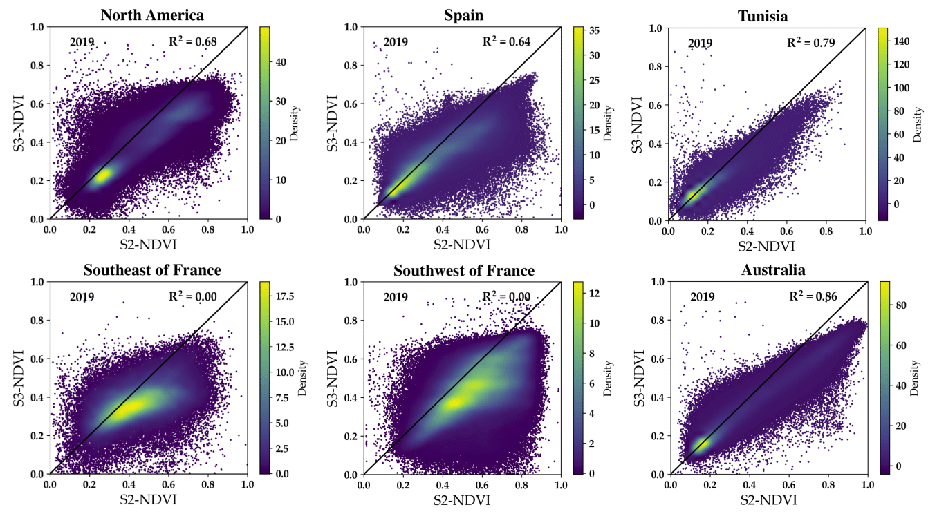
Figure 2 Correlation between S2 and S3 NDVI at 1 km grid scale for the six study regions from January to December 2019.

Then, remotely sensed time series of anomalies in a 35 d time window were also compared to those of the in situ measurements in terms of R. They were derived as follows:

$$\begin{array}{}\text{(2)}& \begin{array}{rl}& {\mathrm{SM}}_t^{\mathrm{a}}=\left({\mathrm{SM}}_t-{\mathit{\mu }}_t\right)/{\mathit{\sigma }}_t\\ & {\mathit{\mu }}_t=\mathrm{1}/N\times \sum _{n=t_{\mathrm{1}}}^{t_{\mathrm{2}}}{\mathrm{SM}}_n\\ & {\mathit{\sigma }}_t=\sqrt{\mathrm{1}/(N-\mathrm{1})\times \sum _{n=t_{\mathrm{1}}}^{t_{\mathrm{2}}}{\left({\mathrm{SM}}_n-\mathit{\mu }\right)}^{\mathrm{2}}},\end{array}\end{array}$$

where ${\mathrm{SM}}_t^{\mathrm{a}}$ and SM_t are the SM and anomalies values at time t, respectively. N is the number of observations from t minus 17 d (t₁) to t plus 17 d (t₂).

Finally, the HR datasets (S²MP_S1S2, S²MP_S1S3, CoperSSM, CoperSWI, and SMAPS1) were evaluated against in situ measurements (R, bias, and SDD with P values below 5 %) after aggregation at 25 km resolution (same grid as that of CCISM) in order to compare their performances to the CR data at a comparable resolution.

4 Results

4.1 Sentinel-3 versus Sentinel-2 NDVI

S2 and S3 NDVI were compared in each region of study at 1 km grid scale in terms of R² as scatterplots in Fig. 2. High R² is observed in Australia (0.86) and Tunisia (0.79), and moderate values are found in North America (0.68) and Spain (0.64). No significant correlation is observed in the southwest and southeast of France. The results indicate that, in dry regions such as in Australia, Tunisia, and North America, a high correlation exists between S2 and S3 NDVI, whereas a low correlation is present in temperate areas with patchy land covers such as in the south of France. For all the study regions, S3 NDVI saturates between 0.6 and 0.7, whereas S2 NDVI reaches higher values between 0.8 and 0.9. The difference could mainly be due to the mixture of surface reflectances from different land cover classes within the 1 km S3 NDVI.

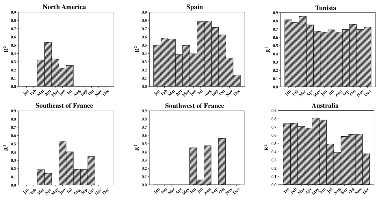
Figure 3 Correlation between S2 and S3 NDVI at 1 km grid scale each month from January to December 2019 for the six study regions. For months with no bars, it means that there is no correlation between S2 and S3 NDVI.

Figure 3 shows the distribution of R² between S2 and S3 NDVI as a function of the months for each region. In general, higher correlations are obtained in the summer season (dry periods) than in winter and spring (humid periods). For example, R² between S2 and S3 NDVI is only high (0.72) from January to June (summer and autumn seasons) in Australia. In North America, from March to July, R² is between 0.25 and 0.53, whereas no significant correlation between S2 and S3 NDVI is found for the other months. In the southwest and southeast of France, no correlation is found for most of the months, except in summer (June, July, and August). On the one hand, the highest NDVI values are found in winter and spring seasons due to the development of the vegetation cycles. On the other hand, summer seasons usually show lower NDVI values that correspond to bare soil conditions, except in the presence of irrigated summer crops. Thus, S2 and S3 NDVI are highly correlated for low NDVI values (usually in summer). However, the correlation decreases for high NDVI values because of the peak of the vegetation development (in spring).

4.2 S²MP_S1S3 comparison to S²MP_S1S2

Figure 4 shows R, bias and SDD between S²MP_S1S2 and S²MP_S1S3 for the six study regions. A very good agreement between the two datasets was found in all the regions with R≥0.9, bias ≤0.04 m³ m⁻³ (S²MP_S1S3 minus S²MP_S1S2), and SDD≤0.03 m³ m⁻³ for most of the areas. However, some differences in terms of bias can be seen between the two datasets in the northwest of the Spanish region (Fig. 4c), in the areas with significant forests cover in the region southwest of France (Fig. 4i), and in narrow areas of the Tunisian region (Fig. 4f).

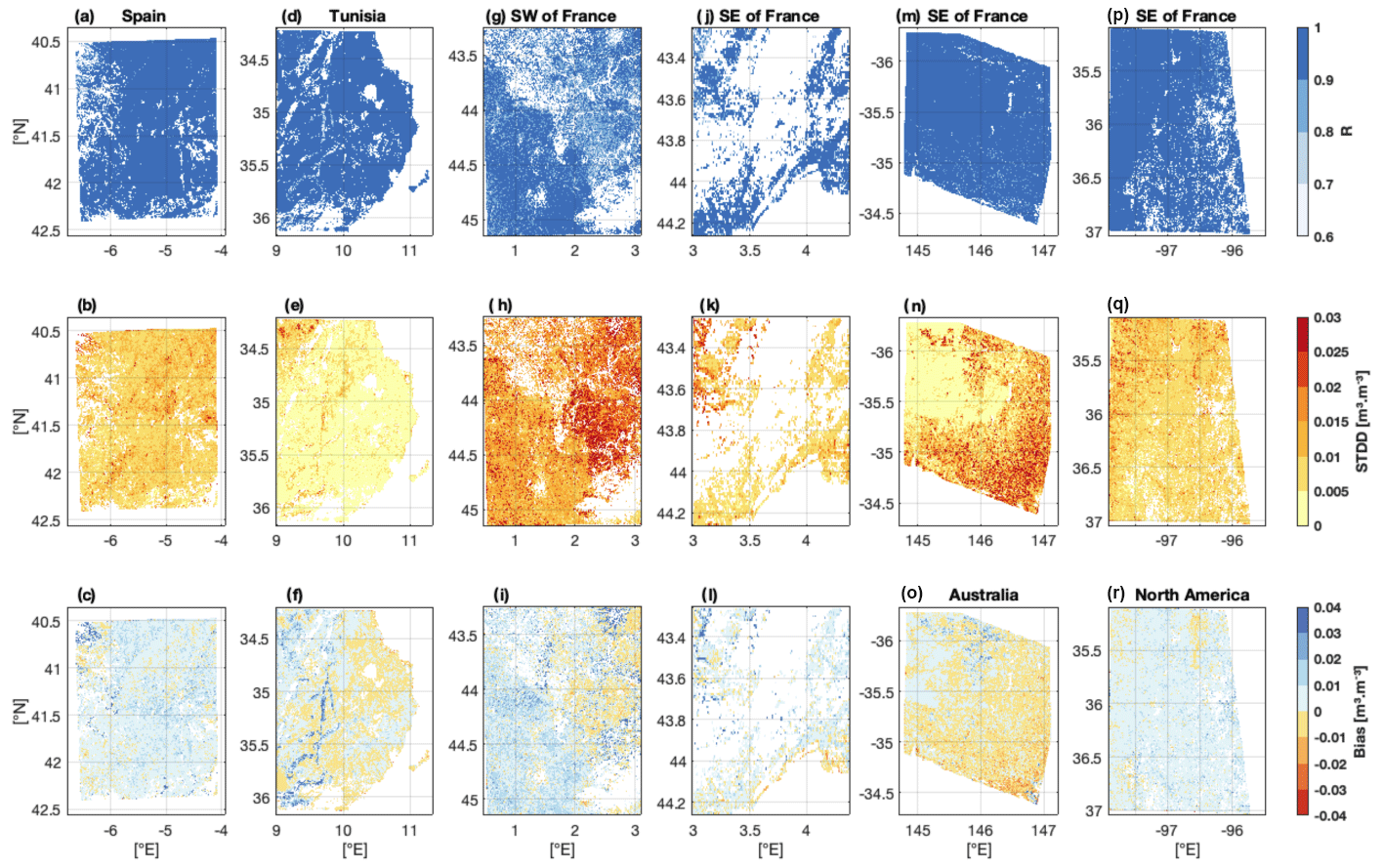
Figure 4 Comparison of S²MP_S1S3 with respect to S²MP_S1S2 over the regions of study in terms of Pearson correlation (R), bias (S²MP_S1S2 minus S²MP_S1S3), and standard deviation of the difference (SDD) in m³ m⁻³. The analysis was performed from January to December 2019.

The somewhat higher differences in the Spanish region and in the region southwest of France are seen over pixels covered by forests, with a small fraction of croplands and herbaceous vegetation (see the Spanish region in Fig. 1b and c). The somewhat larger differences in some narrow areas of Tunisia are due to heterogeneous land cover around several river basins with rolling topography, sparse forests, and grasslands.

As discussed above, these small differences were expected due to the differences seen between S3 and S2 NDVI (Sect. 4.1) and the different way of aggregating the S1 backscatter coefficients (Sect. 3.1). However, taking into account the overall very good agreement between S²MP_S1S2 and S²MP_S1S3, for the sake of simplicity and clarity, in Sect. 4.3 only S²MP_S1S3 is compared to the other HR datasets.

4.3 General comparison of S²MP_S1S3 against the HR SM datasets

Figures 5–7 present the comparison of S²MP_S1S3 against CoperSSM, CoperSWI, and SMAPS1 over the six study regions in terms of bias, SDD, and R, respectively. Some diagonal structures can be seen in the maps comparing S²MP_S1S3 to CoperSSM in Spain and in the southwest of France. These artifacts, most pronounced in the correlation maps and also present in the bias and SDD maps, come from the CoperSSM data, as previously discussed by Bazzi et al. (2019). Indeed, the artifacts are seen on the sub-swaths of the S1 product, showing a big difference between the SM estimations in the CoperSSM at the same SM estimation date. Bazzi et al. (2019) showed that the difference in the SM estimation at both sides of the sub-swath at a given date of the CoperSSM map can reach 0.11 m³ m⁻³.

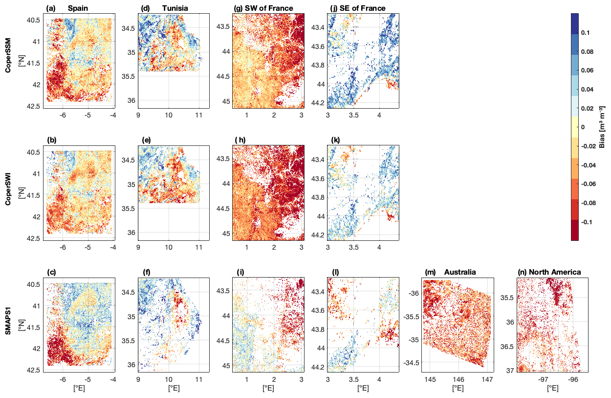
Figure 5 Comparison of S²MP_S1S3 with respect to CoperSSM (S²MP_S1S3 minus CoperSSM), CoperSWI (S²MP_S1S3 minus CoperSWI), and SMAPS1 (S²MP_S1S3 minus SMAPS1) over the regions of study in terms of bias (in m³ m⁻³). The analysis was performed from January to December 2019.

4.3.1 Comparison of the order of magnitude

According to Fig. 5, S²MP_S1S3 shows a bias in the range from −0.1 to 0.1 m³ m⁻³ with respect to the other HR products over most of the pixels within the six regions of study. However, there are areas in the domains of Spain, Tunisia, and southeast of France where S²MP_S1S3 shows a dry bias of an absolute value larger than 0.1 m³ m⁻³. This is also particularly the case in the southwest of France, with respect to CoperSSM and CoperSWI, and in Australia and North America, with respect to SMAPS1n. For these regions and HR datasets, the bias is negative over the whole area. For all the other combinations of regions and HR products, the bias values are both positive and negative. In general, there is no clear relationship between the sign of the bias and the dominant land cover class. However, in the case of the comparison between S²MP_S1S3 and SMAPS1 in the region in the southwest of France, the bias distribution is split in two (Fig. 5i). A wet bias is observed in the western part of the region, corresponding to forests areas with low fractions of croplands and herbaceous vegetation, while a dry bias is found in the eastern part, corresponding to areas dominated by croplands (Fig. 1b and c). In addition, the dry bias observed in the eastern part of the Tunisian region corresponds to an area of salted lakes, whose water and moisture contents can vary significantly according to climate.

Figure 6 shows that the SDD values of S²MP_S1S3, with respect to CoperSSM and CoperSWI, are lower than 0.06 m³ m⁻³ over almost all of the pixels within the four regions for which the Copernicus datasets are available. Higher values close to 0.08–0.10 m³ m⁻³ between S²MP_S1S3 and CoperSSM are found in the southwestern part of the southwest region of France. The SDD obtained between S²MP_S1S3 and SMAPS1 are comparable to those obtained with respect to the Copernicus datasets. However, values reaching 0.08–0.12 m³ m⁻³ are more often found, in particular, in the western part of the Spanish region and are sparse in the southwest and southeast of France. In Australia and North America (Fig. 6m and n), the SDD with respect to SMAPS1 is quite similar to those found in Spain, Tunisia, and France (Fig. 6c, f, i and l), where values can reach ∼0.08–0.12 m³ m⁻³ in the southeastern and western parts of the Australia and North America regions, respectively. There is no clear and unique relationship with the dominant land cover class. For instance, the SDD with respect to SMAPS1 in the southwest of France is higher over the forests than over the cropland-dominated areas, while in the North America region, the SDD was found to be lower over the forests (see Fig. 1b and c).

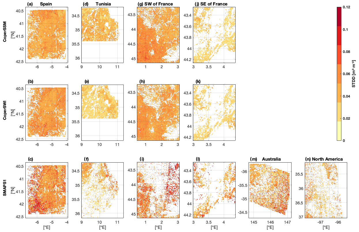
Figure 6 Comparison of S²MP_S1S3 with respect to CoperSSM, CoperSWI, and SMAPS1 over the regions of study in terms of standard deviation of the difference (SDD; in m³ m⁻³). The analysis was performed from January to December 2019.

4.3.2 Comparison of the temporal dynamics

Overall, S²MP_S1S3 and CoperSSM show a high correlation (above 0.7–0.8) over almost all the pixels within all the regions of study (Fig. 7a, d, g, and j). In contrast, lower values are found for the correlation between S²MP_S1S3 and CoperSWI (Fig. 7b, e, h, and k) and between S²MP_S1S3 and SMAPS1 (Fig. 7c, f, i, l, m, and n). R rarely exceed 0.7, and values lower than 0.6 are observed in many large areas.

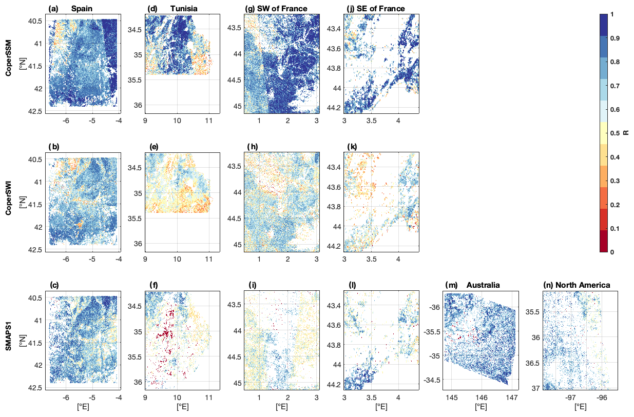
Figure 7 Comparison of S²MP_S1S3 with respect to CoperSSM, CoperSWI, and SMAPS1 over the regions of study in terms of Pearson correlation (R). The analysis was performed from January to December 2019.

In the Spanish region, the highest R values are obtained in the areas dominated by croplands. The lowest values are found in the northwest over heterogeneous pixels dominated by forests (Fig. 1b and c). Similar spatial features are observed in the three maps comparing S²MP_S1S3 to CoperSSM, CoperSWI, and SMAPS1 (Fig. 7a–c). However, lower R values are found with respect to SMAPS1 and CoperSWI. In addition, the comparison with CoperSWI shows R below 0.5 in a few spots in the south and in the center of the region.

In Tunisia (Fig. 7d–f), the correlation values obtained in the north are quite good, with values of 0.8–0.9 with respect to CoperSSM. The R values drop in the southeast and southwest to values lower than 0.5. The decrease in the southwest can be partly explained by the proximity of coasts, where mixed land cover pixels include urban areas (Fig. 1b). The correlation with respect to CoperSWI (Fig. 7e) is only higher than 0.5 for the regions where the 1 km² pixels are dominated by croplands. The comparison between S²MP_S1S3 and SMAPS1 results in a large range of correlations. Only the northernmost areas dominated by croplands show correlations above 0.6 (Fig. 1b and c). R close to 0.4–0.5 are found in the eastern and western parts of the region. Values lower than 0.2 are observed in the center of the region over heterogeneous pixels around several river basins that were also highlighted in Sect. 4.2 with Fig. 4f.

In the region southwest of France (Fig. 7g–i), the distribution of R is quite homogeneous over the whole area and does not vary significantly, according to the pixels dominated by croplands or by forests (Fig. 1b). The R values with respect to CoperSSM are mainly above 0.8 over most of the pixels, while the values drop to 0.5 with respect to CoperSWI. The comparison between S²MP_S1S3 and SMAPS1 shows R values closer to 0.6 in general, but really low correlation values (below 0.2) appear over several pixels. The same pattern is observed in the region southeast of France (Fig. 7j–l), but correlations are only significant over areas dominated by croplands.

R values between S²MP_S1S3 and SMAPS1 reach 0.7–0.8 in Australia and North America (Fig. 7m, n), with no clear relationship to the land cover type.

4.3.3 Comparison over areas dominated by croplands and herbaceous vegetation

To obtain further insight into the analysis over croplands and herbaceous vegetation, S²MP_S1S3 was exclusively compared to CoperSSM, CoperSWI, and SMAPS1 over pixels where one of these two land cover classes is dominant. For each region and land cover, a set of metrics (R, bias, and SDD) is computed in two ways. One set is computed by only taking into account the pixels covered by less than 75 % of croplands or herbaceous vegetation. The other set is computed by only taking into account pixels covered by at least 75 % of croplands or herbaceous vegetation. The results are summed up in Table 2.

Table 2 Comparison of S²MP_S1S3 with CoperSSM, CoperSWI, and SMAPS1, in terms of R, bias, and SDD, over 1 km² pixels, where croplands or herbaceous vegetation are the dominant land cover classes, respectively. The metrics are also derived according to the degree of coverage of the land cover. One set of metrics is computed by considering only pixels covered by less than 75 % of croplands or herbaceous vegetation. Another set of metrics is computed by considering only pixels covered by at least 75 % of croplands or herbaceous vegetation. The analysis was performed from January to December 2019.

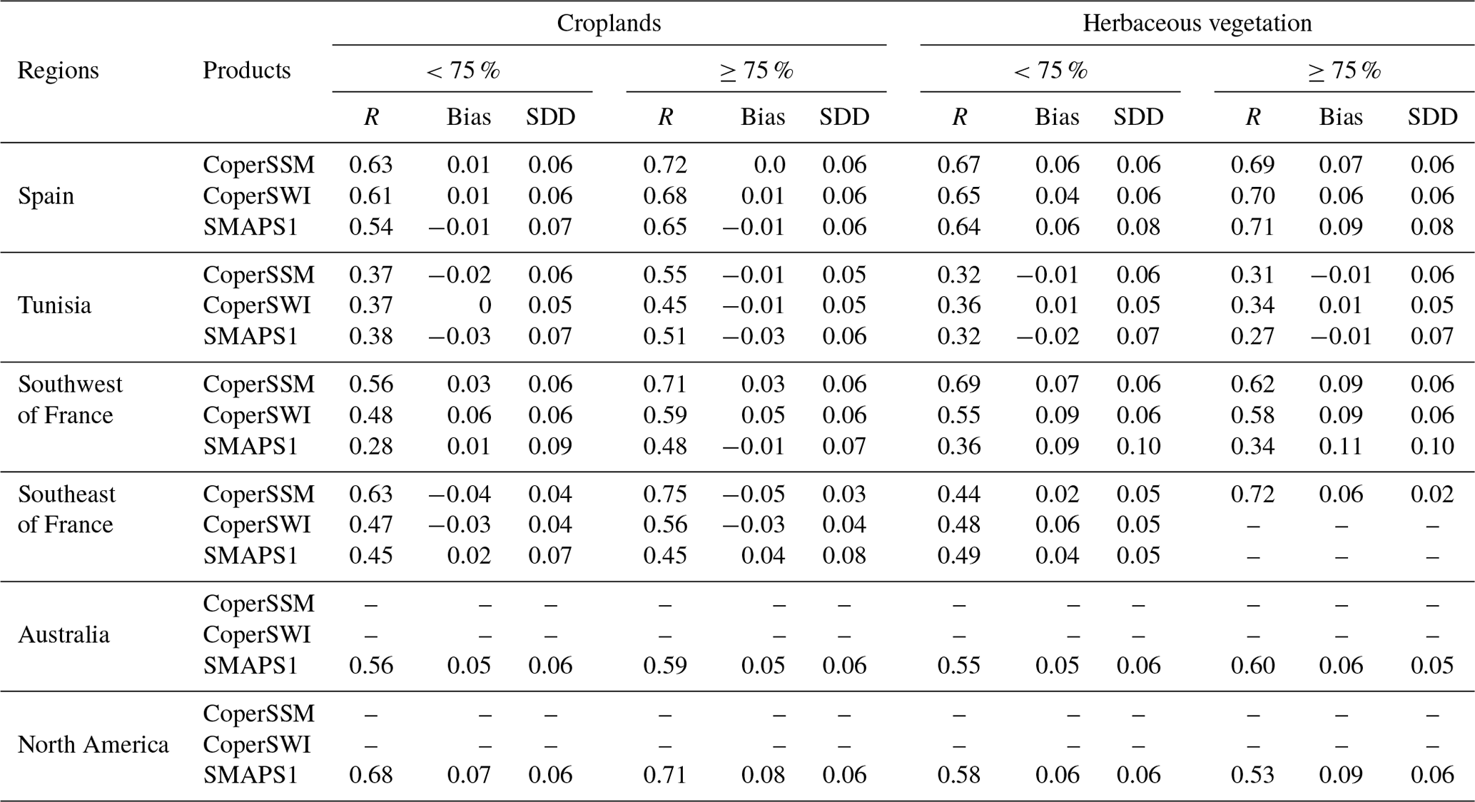
Over pixels in Europe (Spain, Tunisia, and France), where croplands represent less than 75 % of the area, S²MP_S1S3 is better correlated to CoperSSM than CoperSWI and SMAPS1. In general, high R values are found in Spain (0.54–0.63), moderate values (0.28–0.63) are observed in France, and low values are found in Tunisia (0.37–0.38). In addition, R values obtained in Australia and North America with respect to SMAPS1 are comparable to those found in Spain. Absolute bias between S²MP_S1S3 and the three HR datasets in Spain (0.01 m³ m⁻³) are lower than or similar to those found in the other regions. The strongest absolute bias is observed in North America, with respect to SMAPS1, with 0.07 m³ m⁻³. According to the SDD values, no particular trend is observed over the six regions of study, and values range from 0.04 to 0.09 m³ m⁻³. For most of the regions and comparisons, the correlation values significantly increase (+0.05–0.1) over pixels that contain at least 75 % of croplands. In overall, absolute bias and SDD values remain similar, but sometimes there is a slight decrease (−0.01 m³ m⁻³).

Taking into account pixels where herbaceous vegetation represent less than 75 % of the area, S²MP_S1S3 is only better correlated to CoperSSM in Spain and in the southwest of France. In general, high R values are found in Spain (0.64–0.67), moderate values (0.36–0.69) are observed in France, and low values are found in Tunisia (0.32–0.36). In addition, R values obtained in Australia and North America with respect to SMAPS1 are comparable to those found in the southwest of France. Absolute bias between S²MP_S1S3 and the three HR datasets in Tunisia (0.01–0.02 m³ m⁻³) are lower than or similar to those found in the other regions. The strongest absolute biases are observed in the southwest of France, with 0.09 m³ m⁻³ for CoperSWI and SMAPS1, respectively. The SDD is higher with respect to SMAPS1 and can reach 0.07, 0.08, and 0.10 m³ m⁻³ in Tunisia, Spain, and in the southwest of France, respectively. In contrast with croplands, the correlation values do not systematically increase over pixels that contain at least 75 % of herbaceous vegetation. There is no significant change concerning the SDD, and overall, the absolute bias increases with respect to almost all of the HR datasets (+0.01–0.04 m³ m⁻³).

It is noteworthy that the bias is significantly higher over herbaceous vegetation than over croplands in Spain and in the southwest of France, while the SDD is quite similar, regardless of the region of study. In addition, higher R values are found over herbaceous vegetation in Spain. In Tunisia, the correlation and absolute bias values are among the lowest, both over croplands and herbaceous vegetation. Low absolute biases can be partly explained by the fact that the region is really dry, with desert areas, implying a small SM dynamic range with very low values regardless of the estimation algorithm used.

4.4 Evaluation against in situ measurements

Table 3 presents the evaluation of the different CR and HR SM products with respect to in situ measurements in terms of bias, SDD, and R of the original time series, as well as the Pearson correlation of the anomalies' time series (R^a). In addition, Fig. 8 shows examples of the time series of the different HR and CR datasets at six in situ stations used in this study (one for each region).

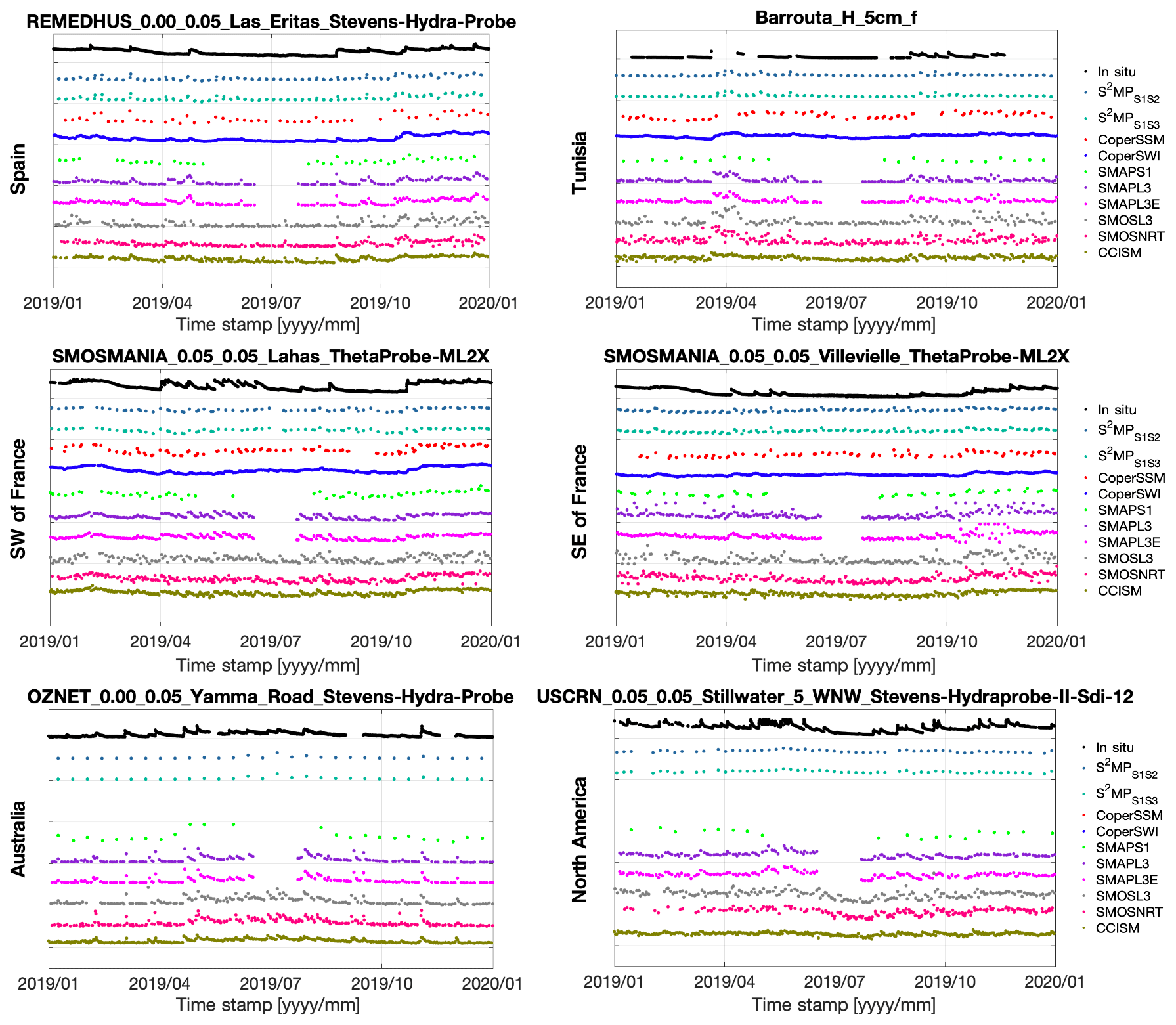
Figure 8 Examples of SM time series from the different HR and CR datasets at six in situ stations (one for each region).

Table 3 Evaluation of the HR and CR SM time series against in situ measurements in terms of the Pearson correlation (R; R^a), bias (remotely sensed minus ground-based SM in m³ m⁻³), and standard deviation of the difference (SDD in m³ m⁻³). The metrics were computed by taking into account the six regions of study, and only the median values are shown here. The asterisk^* indicates the HR datasets averaged at 25 km resolution. The analysis was performed from January to December 2019.

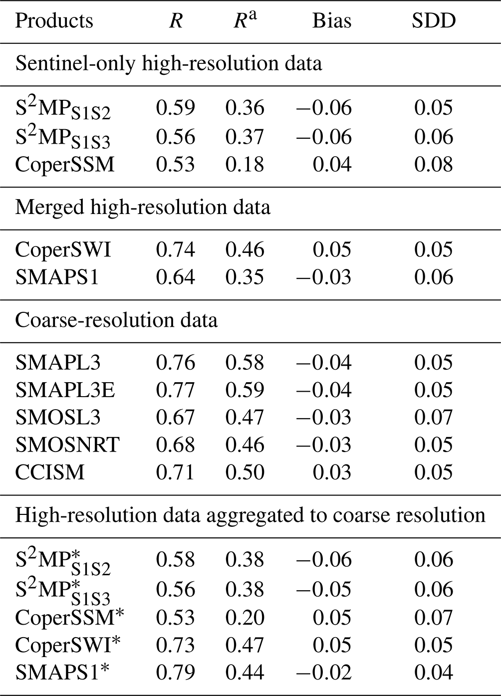
The highest absolute biases with respect to in situ measurements are obtained for S²MP_S1S2 and S²MP_S1S3, with −0.06 m³ m⁻³, closely followed by CoperSWI, with 0.05 m³ m⁻³. SMOSNRT, SMOSL3, CCISM, and SMAPS1 show the lowest absolute biases, with 0.03 m³ m⁻³.

The highest SDDs with respect to in situ measurements are obtained for CoperSSM (0.08 m³ m⁻³) and SMOSL3 (0.07 m³ m⁻³). The other datasets show comparable SDDs, with 0.05 or 0.06 m³ m⁻³.

In general, higher correlation values are obtained for the CR data (0.67–0.77) than for the HR data (0.53–0.74). The lowest correlations are found for the Sentinel-only HR datasets, with 0.53 for CoperSSM, 0.56 for S²MP_S1S3, and 0.59 for S²MP_S1S2. Concerning the HR data obtained from merging approaches, SMAPS1 still shows a value lower than the CR datasets, with 0.64, but CoperSWI shows the third-best value, with 0.74, following SMAPL3E (0.77) and SMAPL3 (0.76).

Regarding the correlation of the anomalies time series, SMAPL3E and SMAPL3 obtain the highest R^a with respect to in situ measurements, with 0.59 and 0.58. CoperSSM, S²MP_S1S2, SMAPS1, and S²MP_S1S3 show the lowest R^a, with 0.18, 0.36, 0.35, and 0.37, respectively.

The CR time series have a temporal revisit roughly 5 times higher than those from S²MP_S1S2, S²MP_S1S3, CoperSSM, and SMAPS1 (Fig. 8). In order to understand if the low temporal revisit of the HR data affects their performances against in situ measurements, one observation out of five was removed from the CR time series, and the metrics were re-computed (not shown). However, no significant differences in terms of R, bias, and SDD were found.

The performances of the two Sentinel-only HR datasets averaged at 25 km resolution (S${}^{\mathrm{2}}{\mathrm{MP}}_{\mathrm{S}\mathrm{1}\mathrm{S}\mathrm{2}}^{*}$, S${}^{\mathrm{2}}M{P}_{S\mathrm{1}S\mathrm{3}}^{*}$, and CoperSSM^*) with respect to in situ measurements are comparable to the performances obtained for the original 1 km datasets (S²MP_S1S2, S²MP_S1S3, CoperSSM, and CoperSWI^*). In contrast, for the SMAPS1^* dataset, which is a downscaled product, the correlation increases from 0.64 at 1 km resolution (SMAPS1) to 0.79 at 25 km resolution, which is the highest correlation found among all the datasets. In addition, the SDD and bias slightly decrease. R^a also increases from 0.35 at 1 km resolution to 0.44 at 25 km resolution, but it does not reach the values of R^a obtained for the SMAP-only products (SMAPL3 and SMAPL3E with 0.58–0.59).

5 Discussion

S²MP, S²MP_S1S3, CoperSSM, CoperSWI, and SMAPS1 are all HR datasets that were produced with different approaches. Two products were obtained by merging S1 data with ASCAT (CoperSWI) and SMAP (SMAPS1), respectively. S²MP and CoperSSM are based on Sentinel only. The last one is computed from local temporal variations in the S1 backscatter coefficients time series, following the method of Wagner (1998). In contrast, S²MP provides SM estimates derived from a NN that uses a database gathering backscatter coefficients and HR NDVI from Sentinel as inputs. The NN was initially trained on a synthetic database containing backscatter coefficients and surface characteristics such as SM and vegetation status (approximated by NDVI) that were predicted from electromagnetic modeling.

Initially, the S²MP algorithm by El Hajj et al. (2017) was only providing SM estimates over croplands at 10 m resolution, using NDVI derived from S2 optical images. In the framework of this study, the algorithm has been extended to provide SM estimates at 1 km resolution, also over herbaceous vegetation areas, and S2 was replaced by S3. However, despite the different ways of aggregating the S1 radar signal and the differences between S3 and S2 NDVI (Sect. 4.1 with Figs. 3 and 2), S²MP_S1S2 and S²MP_S1S3 are in very good agreement over the six study regions (Sect. 4.2 with Fig. 4). Thus, these results imply that it is possible to replace S2 with S3 in the S²MP approach without losing skill. In addition, although the higher temporal revisit of S3 compared to S2 does not allow the S²MP algorithm to provide SM estimates more frequently because the effective revisit is that of S1 (see Fig. 8), the production of the SM daily maps using S3 instead of S2 is easier and faster. S2 and S3 NDVI are derived from optical measurements remotely sensed from space that are highly dependent on the cloud cover situation. Both S2 or S3 NDVI can be unreliable during long rainy or cloudy periods (>15 d) over specific regions. However, the higher temporal revisit of S3 allows the instruments on board S3 to retrieve more optical images without cloud conditions than those on board S2. This results in a better estimation of the vegetation cycle through the NDVI computation. Finally, fewer processing steps are required thanks to the availability of NDVI estimates already provided in the 1 km VEGETATION-like product from Copernicus (see Sect. 2.1.3).

According to Bazzi et al. (2019), the S²MP algorithm tends to provide unreliable SM estimates when the NDVI used exceeds 0.7. NDVI above this value corresponds to well-developed vegetation, and even if it is more common to have NDVI lower than 0.7 with S3 than with S2 (Fig. 2) due to averaging effects, using S3 NDVI does not solve the problem. Indeed, in the particular cases of well-developed vegetation, the problem does not arise from the S2 of S3 NDVI itself but from the C-band SAR signal, which fails to penetrate the vegetation cover.

Regarding the comparisons between the HR datasets in Sect. 4.3, S²MP_S1S3 shows a temporal dynamic closer to those of CoperSSM, CoperSWI, and SMAPS1 over semi-dry areas such as in Spain, North America, and Australia. However, the correlation drops significantly over very dry zones (Tunisia). Over semi-humid areas (France), the temporal dynamic between S²MP_S1S3 and CoperSSM is in better agreement than with respect to CoperSWI and SMAPS1. The order of magnitude (bias and SDD) between S²MP_S1S3 and the other HR datasets is quite similar, regardless of the study region, the land cover, or the climate zone (rather dry or humid). In addition, it is noteworthy to highlight that differences in terms of bias and SDD are not systematically reduced over homogeneous pixels covered by croplands or herbaceous vegetation. This means that inherent biases exist between the algorithms, and they might persist over other land cover classes such as over forests (if the S²MP approach is extended to forests).

At the moment, by construction, the S²MP algorithm starts being out of its application domain when considering pixels dominated by forest cover. This is also the case for the change detection approach used to produce CoperSSM. Indeed, the SM indices computation does not currently account for vegetation dynamics, which can lead to biases over areas covered by seasonal and dense vegetation. In addition, for most applications, the CoperSSM indices and those from CoperSWI should be transformed into SM time series, and this will be problematic without reference SM values under forests to scale them. Therefore, an extension of the S²MP algorithm to forest areas would definitely be interesting to provide HR SM mapping over large regions inside and outside of Europe.

In this study, most of the SM measurements used from the ground stations were representative of croplands and herbaceous regions. Hence, the relative performances of the HR datasets (S²MP, CoperSSM, CoperSWI, and SMAPS1) were not assessed over dense vegetation areas.

In addition, slightly better results of S²MP_S1S3, with respect to in situ measurements, compared to those of CoperSSM were found, except for the bias (Table 4).

Table 4 Evaluation of the HR and CR SM time series against in situ measurements in terms of Pearson correlation (R; R^a), bias (remotely sensed minus ground-based SM in (m³ m⁻³) and standard deviation of the difference (SDD in m³ m⁻³). The metrics were computed by taking into account the six regions of study, and only the median values are shown here. The asterisk^* indicates the HR datasets averaged at 25 km resolution. The analysis was performed from January to December 2019.

SM estimates using the S²MP algorithm were already evaluated against in situ measurements, along with other HR and CR datasets, by El Hajj et al. (2018) and by Bazzi et al. (2019). In El Hajj et al. (2018), the authors found that S²MP_S1S2 shows a lower correlation with respect to in situ measurements than SMAPL3 and SMAPL3E but higher than SMOSNRT, SMOSL3, and SMAPS1. In contrast, in the current study, the S²MP_S1S2 shows a lower correlation with in situ measurements than all the other HR and CR products. However, in El Hajj et al. (2018), SM estimates from the S²MP algorithm were only derived over croplands, while in our study, the SM estimation was performed both over croplands and herbaceous vegetation. Moreover, their analysis was only carried out in the south of France during a different time period (from January 2016 to June 2017). In Bazzi et al. (2019), the authors found that S²MP_S1S2 is better correlated to in situ measurements than CoperSSM. According to the results of our study (Table 4), higher correlations are also obtained for S²MP_S1S2. In addition, it is interesting to note that S²MP_S1S2 and S²MP_S1S3 show similar performances with respect to in situ measurements.

Taking into account the evaluations of all the HR and CR products (Table 4), HR-merged datasets (SMAPS1 and CoperSWI) provide better estimations or temporal agreement with respect to in situ measurements than the HR Sentinel-only ones (S²MP_S1S2, S²MP_S1S3, and CoperSSM). However, they still show performances similar to or lower than the CR datasets (Table 4). This can be partly explained by the fact that the HR datasets provide SM estimates using C-band measurements, while the CR datasets used in this study are computed using L-band measurements. Indeed, SMOS and SMAP were specifically designed to measure surface SM, which was not the case for the Sentinel satellites. Regarding the higher performances of the CR datasets over the HR ones, with respect to in situ measurements, Bauer-Marschallinger et al. (2019) also demonstrated that 25 km resolution SM estimates from ASCAT were better correlated to in situ measurements within the Italian Umbria region than those of the 1 km resolution CoperSSM. The results of our study are also in perfect agreement with the findings by Ojha et al. (2021), who showed, over several regions in France and Spain, that two merged products, SMAPS1 and SMAP + DISPATCH (Merlin et al., 2012), were better correlated to in situ measurements than CoperSSM. Finally, it is noteworthy that the performances of SMAPS1 aggregated from 1 to 25 km resolution (CR) increase to values similar to those of SMAPL3. This implies that the gain in resolution brought by merging data of different resolutions comes at the expense of introducing uncertainties in the resulting HR dataset.

Obviously, this study was limited to comparisons over six regions of 10⁴ km² within a 1-year time period, so the results cannot be straightforwardly extended to a global scale. However, the results of the study show that the use of S3 NDVI as input to the S²MP algorithm leads to SM estimates comparable to those obtained with S2 NDVI. However, HR SM estimates do not necessary lead to better performances than CR SM estimates, with respect to in situ measurements. In particular, retrieval algorithms only based on Sentinel measurements (S²MP and CoperSSM) need improvements before reaching performances comparable to those used with the HR-merged or CR datasets. However, the S²MP datasets still have two advantages over CoperSSM. They currently show better performances against in situ measurements and are able to provide SM estimates outside of Europe. Hence, it would be interesting to extend the S²MP algorithm to all the types of land cover and to provide SM estimates over the entire globe. The objective would be to produce the first Sentinel-only SM dataset available at a global scale and to perform a deeper comparisons against SMAPS1 over large areas. However, the estimation of SM using the S²MP algorithm outside of Europe would remain challenging due to the inhomogeneous spatial and temporal coverage of S1 (Bauer-Marschallinger et al., 2019).

6 Conclusions

The goal of this study was to adapt the S²MP approach, originally designed to retrieve SM at 10 m resolution over agricultural fields, to a 1 km resolution, which allows the replacement of S2 by S3, and to significantly improve the NDVI temporal sampling. In addition, the approach was extended to herbaceous land cover areas and tested in six regions over four continents to assess its performances beyond previous evaluations in southern France.

A very good agreement was found between the S1 + S3 and the S1 + S2 S²MP maps for the V regions (R≥0.9, bias ≤0.04 m³ m⁻³, and SDD≤0.03 m³ m⁻³), meaning that it is possible to replace S2 by S3 NDVI.

The S²MP maps were then compared to those of the 1 km surface SM product provided by CGLS (CoperSSM), which is also a Sentinel-only-based dataset. In contrast to S²MP, CoperSSM provides local indices of SM variations. For many applications, they have to be scaled against a reference to transform the variations to actual SM in volumetric units (m³ m⁻³) before being used. Then, S²MP was also compared to two HR-merged datasets, that is (i) the SWI dataset from CGLS, combining S1 and ASCAT measurements (CoperSWI), and (ii) the SMAP + S1 dataset. As for the surface SM dataset, the SWI data had to be scaled into absolute SM values. CGLS products only provide estimates over the European continent and the Mediterranean basin.

Overall, the S²MP dataset is better correlated to the 1 km surface SM product provided by CGLS over the four regions of study in Europe (R∼0.7–0.8). Over almost all of the pixels within the six regions, the SDD between S²MP and the other HR datasets is lower than 0.06 m³ m⁻³. In addition, the bias differs significantly inside the same region and can be strongly dry or wet (±0.1 m³ m⁻³). The correlations between S²MP and the other HR datasets improve over croplands when the 1 km pixels become homogeneous, but a similar behavior was not clearly found for the other metrics (SDD and bias) or over pixels where the dominant land cover class is herbaceous vegetation.

The S²MP datasets were also evaluated with respect to in situ measurements, along with the three other HR datasets, and with coarser-resolution datasets from SMOS, SMAP, and ESA CCI. The coarse-resolution (CR) products show higher correlations ($\mathrm{0.68}\le R\le \mathrm{0.77}$) than the HR datasets ($\mathrm{0.54}\le R\le \mathrm{0.74}$), and the HR-merged datasets showed higher correlations than the HR Sentinel-only ones. S²MP_S1S2 showed the highest bias with respect to in situ measurements, with −0.07 m³ m⁻³. Finally, the SDD differs according to the dataset in addition to the spatial resolution and range from 0.05 (with S²MP_S1S2, for example) to 0.08 m³ m⁻³ (CoperSWI).

In general, these results show that the HR datasets only based on Sentinel (S²MP and CoperSSM) are not as competitive as the other HR-merged and CR datasets with respect to in situ measurements in terms of correlation and bias, but S²MP still presents several advantages. In contrast to the HR data from Copernicus, the S²MP data do not depend on auxiliary data to be scaled into volumetric units and can provide SM estimates outside of Europe. S²MP_S1S2 also shows lower SDD, with respect to in situ measurements, than the Copernicus and the SMAP + S1 datasets. It would be interesting to extend the S²MP to all the types of land cover and to provide SM maps at the globe scale. S²MP_S1S2 would be the first global SM dataset at 1 km resolution only that is based on Sentinel measurements. It would also allow the performing of deeper comparisons against SMAP + S1 over large areas, and S²MP_S1S2 could be used to assess the climate impact at a regional level in the future. However, a remaining challenge is to provide HR SM data with comparable spatiotemporal coverage and retrieval quality across different land cover types than those of the state-of-the-art coarse-resolution products, such as the SMOS, SMAP, and ESA CCI products.