the Creative Commons Attribution 4.0 License.
the Creative Commons Attribution 4.0 License.
 | 14 Mar 2023
Bayesian calibration of a flood simulator using binary flood extent observations
David Charles Bonaventure Lallemant
Computational simulators of complex physical processes, such as inundations, require a robust characterization of the uncertainties involved to be useful for flood hazard and risk analysis. While flood extent data, as obtained from synthetic aperture radar (SAR) imagery, have become widely available, no methodologies have been implemented that can consistently assimilate this information source into fully probabilistic estimations of the model parameters, model structural deficiencies, and model predictions. This paper proposes a fully Bayesian framework to calibrate a 2D physics-based inundation model using a single observation of flood extent, explicitly including uncertainty in the floodplain and channel roughness parameters, simulator structural deficiencies, and observation errors. The proposed approach is compared to the current state-of-practice generalized likelihood uncertainty estimation (GLUE) framework for calibration and with a simpler Bayesian model. We found that discrepancies between the computational simulator output and the flood extent observation are spatially correlated, and calibration models that do not account for this, such as GLUE, may consistently mispredict flooding over large regions. The added structural deficiency term succeeds in capturing and correcting for this spatial behavior, improving the rate of correctly predicted pixels. We also found that binary data do not have information on the magnitude of the observed process (e.g., flood depths), raising issues in the identifiability of the roughness parameters, and the additive terms of structural deficiency and observation errors. The proposed methodology, while computationally challenging, is proven to perform better than existing techniques. It also has the potential to consistently combine observed flood extent data with other data such as sensor information and crowdsourced data, something which is not currently possible using GLUE calibration framework.
- Article
(5219 KB) - Full-text XML
- BibTeX
- EndNote


As floods represent the most costly natural hazard worldwide, the relevance of scientifically informed risk management to aid in mitigating the impact of floods in human environments is of foremost importance (Global Facility for Disaster Reduction and Recovery, 2014; Jha et al., 2012). Furthermore, the characterization of flood risk management as a problem of decision-making under uncertainty is now widely accepted in the research community, and efforts are increasingly being placed in that direction (Hall and Solomatine, 2008; Beven, 2014a). In this line, there is a need to robustly and transparently characterize the uncertainty in all components of a flood risk analysis, particularly in the floodplain inundation model, usually considered deterministic in practice.
This paper focuses on the use of computational simulators of inundation models, a key component in flood risk quantification, that aim to simulate the process by which water flows throughout a floodplain due to riverine bank overflow, water excess from rainfall, large coastal wave heights or any combination of those. This is done by solving a set of flow dynamics equations both in space and time for a given set of initial and boundary conditions and is termed here a flood simulator. Even for a well-defined forcing event (e.g., a known flow discharge, rainfall, or sea-level rise), predictions of the flood process remain largely uncertain due to a combination of (1) errors in observations used for calibration, (2) errors in the simulator structure due to simplifications (also termed model inadequacy), (3) numerical errors in solving the physics-based model (also termed code uncertainty), and (4) residual error as a result of aleatory uncertainties in nature and other unknown unknowns (Kennedy and O'Hagan, 2001). Thus, in line with the uncertainty quantification objectives, several authors in recent decades have highlighted the importance of building probabilistic, rather than deterministic, estimations of physical processes in general and flood processes in particular (Kennedy and O'Hagan, 2001; Goldstein and Rougier, 2004; Moges et al., 2021; Di Baldassarre et al., 2010; Beven, 2014b; Alfonso et al., 2016).
Uncertainty quantification of predictions is obtained through probabilistic calibration of the simulator based on real-world observations of the process output and its boundary conditions. For flood simulators, this was initially done with the use of discharge measurements and water levels at points along the reach (Romanowicz et al., 1996; Werner et al., 2005). With the increased availability of satellite imagery, particularly from SAR (synthetic aperture radar) satellites, to obtain flood extent information (i.e., binary observations) and the increased computational capacity to implement 2D inundation models, spatially distributed observations have been used widely for calibration in the last 20 years. The added value of distributed data and model predictions for inundation modeling has been widely accounted for in the literature (Aronica et al., 2002; Hunter et al., 2005; Werner et al., 2005; Pappenberger et al., 2005; Stephens and Bates, 2015).
The widespread use of distributed observations in uncertainty quantification of flood predictions was also driven by the formalization of the generalized likelihood uncertainty estimation (GLUE) framework by Beven and Binley (1992). Due to its simplicity and ease of implementation, it has been widely used to calibrate probabilistic flood models in the last 2 decades by quantifying uncertainty in simulator parameters (Aronica et al., 2002; Romanowicz and Beven, 2003; Bates et al., 2004; Hunter et al., 2005; Werner et al., 2005; Horritt, 2006; Di Baldassarre et al., 2009; Mason et al., 2009; Di Baldassarre et al., 2010; Kiczko et al., 2013; Wood et al., 2016; Romanowicz and Kiczko, 2016). Its strength does not rely only on its simplicity, but it is also a working alternative for complex cases with “non-traditional error residual distributions”, as explained by Sadegh and Vrugt (2013). In cases like this, formal likelihood functions that fail to capture the complex distribution of the observations can be overly optimistic regarding the uncertainty (Sadegh and Vrugt, 2013; Beven, 2016; Wani et al., 2019).
This inference technique, closely related to the modern approximate Bayesian computation (ABC) methods (Sadegh and Vrugt, 2013), is based on simplified likelihood functions (also termed “pseudo-likelihood”) using summary indicators of the fit between data and observations. This implies that predictions cannot be formally interpreted as probabilities, since the method does not provide a distribution model for the residuals. Furthermore, GLUE implementations do not attempt to capture the spatial structure of the residuals and cannot differentiate between observation errors (typically assumed mutually independent) and model inadequacy errors that usually exhibit a systematic behavior in space and time (Stedinger et al., 2008; Vrugt et al., 2009; Rougier, 2014) (i.e., some locations are systematically over- or under-flooded). As a result, all variability in prediction is characterized through uncertainty in the model parameters, implicitly assuming that, at least, some of the simulator parameters can fit the true process reasonably well in all locations of interest.
Alternatively, the formal Bayesian approach for uncertainty quantification in simulator predictions appears to be a robust framework to cope with many of the limitations of GLUE while transparently and consistently translating the modeler's subjective judgments on uncertainty into probabilities (Rougier, 2014). The seminal work on probabilistic calibration of computational simulators by Kennedy and O'Hagan (2001) proposed a fully probabilistic model building methodology to explicitly account for observation errors, model inadequacy, and parametric uncertainty. This approach, later extended by others (Goldstein and Rougier, 2004; Rougier, 2014), has been widely used in many different disciplines, although its application to inundation models has been mostly restricted to a few cases where flood-depth measurements were available (Hall et al., 2011). The complex statistical properties of spatial binary observations have restricted its widespread implementation in practice. Some researchers have extended this framework to binary observations. Wani et al. (2017), Cao et al. (2018), Chang et al. (2019), and Woodhead (2007) attempted this for inundation models. This latter study, however, did not explicitly account for the model inadequacy, and inferences were focused on binary values (i.e., flooded or non-flooded) rather than on flood depths.
The present work proposes to adapt the fully Bayesian methodology of Kennedy and O'Hagan (2001) to create probabilistic predictions of flood depths using inundation simulators with spatial binary observations of flood extent obtained from SAR satellite imagery and compare it to simpler and more traditionally used methods. The proposed calibration approach aims to do the following:
-
Develop a rigorous and probabilistic framework for inundation model inference. This enables consistent uncertainty propagation through the risk modeling chain using a Bayesian methodology and allows for a consistent integration of data from different sources, such as binary satellite-borne flood extent data, uncensored flood-depth measurements on the ground, or crowdsourced qualitative data.
-
Explicitly account for the deficiencies of the computational flood simulator driven by simplifications in the fluid dynamics equations used, errors in the input data (e.g., elevation map inaccuracies), and/or numerical inaccuracies of the solver. These are explicitly taken into account by the inclusion of an additive, spatially correlated, inadequacy term in predictions.
-
Model errors in data acquisition (i.e., observation errors) explicitly and disaggregated from other uncertainty sources such as model structural deficiencies and input errors.
The proposed approach is built based on the Gaussian process classification theory (see Rasmussen and Williams, 2006), where the physical process acts as the latent variable that is being censored. It can be also found in the literature as a clipped Gaussian process (CGP) model (Oliveira, 2000) or as a particular case of the spatially correlated multivariate probit model with non-linear regressors (Chib and Greenberg, 1998). Several publications can be found where different physics-based simulators were calibrated using censored observations of the real process and statistical inadequacy functions (Wani et al., 2017; Cao et al., 2018; Chang et al., 2019), although no attempt, to the authors' knowledge, has been made to implement this in the context of flood simulators and binary extent observations.
This work is organized as follows. Section 2 provides a review of the general Bayesian framework for the statistical calibration of computational model as proposed by Kennedy and O'Hagan (2001) and describes the three specific calibration approaches used in this paper: (1) the widely used GLUE framework, (2) a fully Bayesian model without inadequacy function, and (3) a fully Bayesian framework including an inadequacy term. Section 3 describes an illustrative one-dimensional example to help understand some of the key implications of using an inadequacy function and binary data for calibration. Section 4 describes a real case study, the data available for calibration, its numerical implementation, and the results from the three models. Section 5 presents a discussion of the key findings and limitations of the proposed approaches in terms of model building, uncertainty quantification, and information content of data. Conclusions and potential paths for future research can be found in Sect. 6.
2.1 Uncertainty framework
Using mathematical models to make inferences about real-world physical systems involve many sources of uncertainty, since (i) the models are always incomplete simplifications of reality, (ii) computational simulators can be numerically imprecise, and (iii) these simulators require inputs that are uncertain (Goldstein and Rougier, 2004). A robust characterization of these uncertainties is, then, necessary to understand the implications of the inferences made. In this context, an uncertainty framework is a mathematical description of the probabilistic relationships between (1) a computational simulator S used to describe a physical system, (2) inferences about the true physical process Y, and (3) observations of that process Z.
In this work, we will use uppercase letters to describe random variables and lowercase letters for their particular realizations. Bold letters indicate some vectorial quantity that, in the case of the spatial processes S, Y, and Z, indicates values at different points in space. For example, Y={Y(x1), Y(x2), …, Y(x3)}. Greek letters will be used for model input parameters.
The simulator is a mechanistic model used to represent a physical process by means of simplifying assumptions of the real world. In the context of flood modeling, this is a computational code that outputs flood depths (and potentially many other parameters) at different points in space S, by solving a set of flow dynamics equations in a given spatial and time domain and for a set of required inputs (see Eq. 1): (1) a set of boundary conditions ν that are considered to vary from event to event and are considered known (either observed or predicted), like the upstream hydrograph or peak flow in the case of a riverine flood scenario, and (2) a set of model's parameters β that are typically unobservable and considered to be fixed for a wide range of contexts by an appropriate calibration procedure (Kennedy and O'Hagan, 2001), such as terrain topography, surface roughness, or Manning's roughness parameters.
A real-world physical process is, however, described by a very complex function relating the input boundary conditions ν and true process output Y. This function is not known (and cannot be known), and the modeler needs to rely on the available simulator that is not, in any case of practical interest, a perfect representation of the true process: Y≠S. To represent this discrepancy mathematically, some researchers (Kennedy and O'Hagan, 2001; Goldstein and Rougier, 2004) have proposed the use of an additive model inadequacy function δ as in Eq. (2).
Finally, observations of the physical process Z at a set of points in space can be obtained through some data-acquisition technique. During flood events, there are different sources of observations such as water level readings from gauging stations in rivers, satellite imaging (particularly SAR imaging) of flood extent, and, more rarely, ground observations of water depths in the floodplain (Di Baldassarre, 2012). In any case, there are two types of observations, uncensored water depth observations (a positive real value) and binary observations (water–no water), that are distinct from those obtained from SAR satellite imagery.
Mathematically, observations can be thought of as noisy versions of the true process Y, typically characterized by some additive error process ε as per Eq. (3) (Kennedy and O'Hagan, 2001; Goldstein and Rougier, 2004). Furthermore, binary observations, on which this work will mostly focus, can be represented as censored versions of the continuous water depth measurements, as seen in Eq. (4).
where 𝟙{condition} is the indicator function that equals 1 when the condition is true and 0 otherwise.
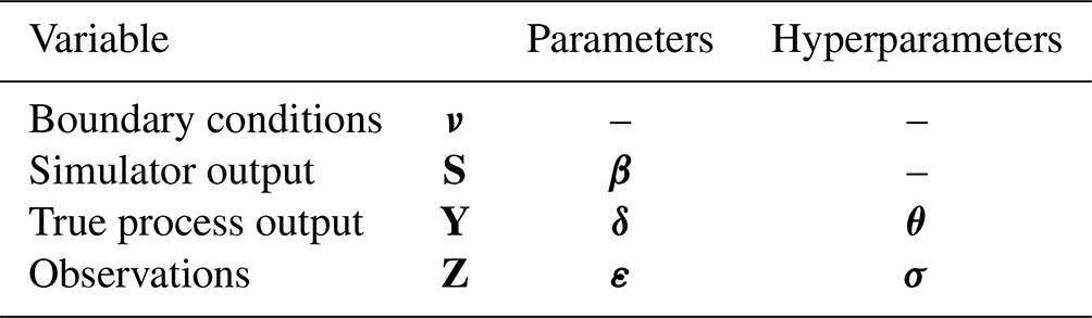
All variables and model parameters introduced so far are summarized in Table 1.
Table 1Summary of variables, parameters, and hyperparameters in the uncertainty framework.
2.1.1 Bayesian inference
The objective of uncertainty quantification is, in this case, to obtain probabilistic predictions of the true process output Y* at spatial locations x* for unobserved boundary conditions ν*. The Bayesian methodology allows us to condition these predictions on previously observed data {z,ν}, also known as calibrated predictions (Gelman et al., 2013). The predictive distribution density can be computed as
The distribution represents the uncertainty in the computation of the simulator outputs at the locations of the new values, also termed code uncertainty in the literature (Kennedy and O'Hagan, 2001). This can be associated with numerical errors in the implementation and solving of the equations of the model but more significantly can arise due to surrogacy of the model by the use of statistical emulators (Carbajal et al., 2017; Jiang et al., 2020). This is useful when the original simulator is computationally expensive to run and doing hundreds or thousands of simulations is not feasible. This will not be the case in this work, so we will assume that the simulator S can be deterministically obtained given its parameters β. That is, has a single probability mass at , and the predictive distribution is reduced to Eq. (6). An application of the use of statistical emulators within the framework described here can be found in Kennedy and O'Hagan (2001) and Hall et al. (2011).
Considering a deterministic computational simulator, and integrating out the terms δ and s in Eq. (5), we obtain
The distribution is the posterior distribution of the simulator parameters β conditioned on observed data and is a representation of the parametric uncertainty of the model. On the other hand, the conditional predictive distribution reflects the uncertainty on new true process predictions for a given simulator output defined by β and for a new event ν*. This is the quantification of model inadequacy and is obtained by integrating over the posterior distribution of the inadequacy term conditioned on data as in Eq. (7).
The posterior distributions of both the inadequacy term δ and simulator parameters β are the core of Bayesian statistics since they define how data are assimilated into new predictions of the true process as given in Eqs. (8) and (9).
The distribution is the joint probability of observations conditioned to a given value of the simulator and the inadequacy terms (also termed conditional likelihood function). That is, it is defined by the distribution of the errors in observations ε. On the other hand, is the probability of obtaining the observed data for a given set of simulator parameters and is obtained by integrating out the inadequacy terms from the distribution in Eq. (8). This is why it is also termed marginal likelihood function here or simply likelihood function. Finally, f(δ) and f(β) are the prior distributions of the inadequacy term and the simulator parameters respectively. This should reflect the modeler's knowledge before obtaining, or disregarding, the available data (Rougier, 2014).
Since the spatial terms δ and ε are high-dimensional random variables, they can result in complex prior distributions with an arbitrarily large number of hyperparameters. It is typical, then, to define parametric joint distributions for each that depend on only two sets of hyperparameters: θ and σ respectively (see Table 1). Parameter selection can be done by fixing these hyperparameters to some values defined by the modeler or assigning some appropriate hyperpriors to each. The posterior distribution of simulator parameters and the likelihood function are extended to include the set of hyperparameters as in Eq. (10). In the same line, the predictive distribution (Eq. 6) and the inadequacy function posterior distribution (Eq. 8) should always be understood as also conditioned on hyperparameters θ and σ.
In this framework, then, a given statistical model is defined by assigning a prior distribution for the inadequacy term, f(δ), and for the observation error (the likelihood function is obtained by integrating out δ from the latter). When no closed-form solution for the distributions exists, approximate sampling schemes, such as Markov chain Monte Carlo (MCMC) (Gelman et al., 2013), are typically used to (i) sample model parameters from Eq. (10), then (ii) sample the inadequacy function from Eq. (8), and finally (iii) sample the true process output (e.g., flood depths) from .
In the next section, two different models within this framework will be analyzed: one with the inadequacy function and one without.
2.2 Statistical models
Given the proposed Bayesian uncertainty framework to obtain calibrated predictions of flood events given past observations, a proper implementation requires the modeler to define probability distributions for the observation error model ε and prior distributions for the model inadequacy δ, and simulator parameters β. Three models are reviewed in this work: (1) the widely used GLUE method (current state of practice), (2) a simple Bayesian model without including an inadequacy term, and (3) a newly proposed Bayesian model including an inadequacy term with a spatially correlated Gaussian process prior.
2.2.1 Model 1: GLUE
GLUE has been, by far, the most widely used approach for the statistical calibration of flood simulators using flood extent data (Aronica et al., 2002; Hunter et al., 2005; Horritt, 2006; Stephens and Bates, 2015; Wood et al., 2016; Papaioannou et al., 2017). In this framework, the marginal likelihood is obtained from a score that ranks each set of β in terms of how “good” they are in predicting the observed data. In this sense, it is only informally a likelihood function, or pseudo-likelihood. It is typical to leave out (i.e., assign a 0 likelihood) those β values for which the score is below some minimum acceptance threshold defined by the modeler. A very high threshold will only accept very few β values with a relatively good fit with the observation but potentially with a larger bias (see Beven, 2014a, b).
The most widely used score function is some modified version of the critical success index (CSI), which penalizes overprediction of flooded pixels (Aronica et al., 2002; Hunter et al., 2005; Stephens and Bates, 2015). This is
where A is the number of correctly predicted pixels, B is the number of overpredicted pixels (predicted flooded observed non-flooded), and C is the number of underpredicted pixels (predicted non-flooded and observed flooded).
To build a likelihood distribution for each value of β from the score in Eq. (11), three steps are typically followed: (1) compute a rescaled F0 score so that it lies in the [0, 1] range to ensure positivity, (2) reject all “non-behavioral” models by assigning F0=0 according to a predefined acceptance threshold (e.g., all models with F<0.5 or the 70 % group with lower F values), and (3) standardize the resulting F scores so that they all integrate to 1. The pseudo-likelihood is, then, defined in Eq. (12).
where .
Posterior samples for the parameters β are typically drawn by assuming a uniform prior, although it is not a requirement of the framework. Values βj are drawn uniformly from the defined range of possible values, and the likelihood is computed for each with the procedure described above. The likelihood values are then used as weights to sample posterior values of β.
Finally, since no inadequacy is considered in this framework δ≡0, true process inferences are obtained directly from the simulator output Y=S for each posterior sample o β. All uncertainty, then, is included in the posterior distribution of the simulator parameters (i.e., parametric uncertainty), and no attempt is made to describe the joint distribution of the discrepancy between observations and simulator outputs (Stedinger et al., 2008).
2.2.2 Model 2: no inadequacy and independent observations
This model considers no inadequacy (i.e., δ≡0) and assumes that observation errors are spatially independent. It is perhaps, the simplest formally Bayesian model for calibrated predictions, and it implicitly assumes that the simulator can reliably capture the spatial structure of the true process. As in the GLUE framework, uncertainty in predictions is characterized by uncertainty in simulator parameters β. Model setup is summarized in Eq. (13).
The likelihood function is given by the distribution of observation errors ε for a given set of hyperparameters σ. Since observations are, in this case, independent binary variables, the likelihood function is just the product of Bernoulli probabilities given as
where pj is the probability that observation Zj=1 and depends on the marginal distribution for the observation error εj.
Different probability distributions for the independent observation errors εj yield likelihood models for the data with distinct properties. Some of the typical ones are as follows:
-
The probit model assumes a Gaussian distribution so that .
-
The logit model assumes a logistic distribution so that .
-
The binary channel model assumes a discrete Bernoulli distribution for εj, where .
For a given set of parameters β and σ, each data point marginally contributes a quantity to the total likelihood. Considering this, we can draw some conclusions on how each error model deals with model predictions when maximizing the likelihood function:
-
Correctly predicted wet (). The marginal contribution is in this case pj. The logit and probit models assign a marginal contribution of and the binary channel model a value of σ1.
-
Correctly predicted dry (). The marginal contribution is in this case 1−pj. The logit and probit models assign a marginal contribution of 0.5 and the binary channel model a value of σ2.
-
Overpredicted (). The marginal contribution is in this case 1−pj. The logit and probit models assign a marginal contribution of and the binary channel model a value of 1−σ1.
-
Underpredicted (). The marginal contribution is in this case pj. The logit and probit models assign a marginal contribution of 0.5 and the binary channel model a value of 1−σ2.
The analysis in the previous paragraph shows that the probit or logit models do not seem reasonable for this type of problem. On the one hand, these models assign the same likelihood to a correctly predicted dry point and an underpredicted point (predicted dry and observed wet). On the other hand, both models seem very inflexible in the sense that they always penalize more overpredicted points than underpredicted ones, and correctly predicted wet points are more “rewarded” than correctly predicted dry points. For these reasons, the binary channel model, although quiet simple, appears to be a more suitable and flexible option in this case (see Woodhead, 2007, for a more detailed discussion on this model). This model also allows for a simple expression to calculate the log-likelihood for a given set of parameters as
where A is the total number of correctly predicted flooded observations, B is the number of overpredicted (i.e., predicted flooded but observed dry) observations, C is the number of underpredicted observations (predicted dry but observed flooded), and D is the number of correctly predicted dry observations.
Since there is no inadequacy, as in the GLUE model, predictive samples of flood depths are obtained from the simulator output for each posterior sample of β.
2.2.3 Model 3: inadequacy function and independent observations
The full model proposed here assumes that the additive inadequacy function δ has a 0-mean Gaussian process (GP) prior with a squared exponential covariance function defined by hyperparameters θ and that observation errors ε follow an independent Gaussian distribution with hyperparameter σ that represents the marginal standard deviation. The use of GPs for the inadequacy is convenient for analytical reasons since Gaussian distributions have well-studied joint and conditional properties but also from a historic perspective since the use of GPs for spatial data regression underlies the first geostatistical techniques, such as kriging (Schabenberger and Gotway, 2005).
This is a generalization of the spatially independent model described in Sect. 2.2.2, in the sense that it assumes that the discrepancy between the simulator output and true process has a spatially correlated structure. The null mean implies that, a priori, it is not known if model inadequacy will be positively or negatively biased. The model setup is described in Eq. (16).
The true process Y is strictly positive and the sum S+δ not necessarily. Thus, the model setup requires the negative values to be rectified with the function , assigning the probability of all negative values to the point y=0 and generating a zero-inflated process (there is a non-zero probability mass at y=0). The spatial structure of the inadequacy function is characterized by a squared exponential kernel (SEK), as per Eq. (17), with a variance parameter θ1 that controls the amplitude of the realization and an inverse length parameter θ2 that controls its roughness (number of crossings of an horizontal axis). For an analysis of the influence of kernel selection in GP regression, refer to Rasmussen and Williams (2006).
Given this model setup, the likelihood of observed data is given by the cumulative multivariate Gaussian function as
where Kθ is the covariance matrix as obtained from kernel (Eq. 17). For observed spatial points x and given hyperparameters θ, the integration limits for each observed point are
Equation (18) gives the likelihood of a multivariate probit model that has been widely used for spatial classification models and which can also be found in the literature as a clipped Gaussian process (CGP) (Oliveira, 2000) or as a spatial generalized linear model (SGLM) (Schabenberger and Gotway, 2005; Berrett and Calder, 2016). It involves the integration of a high-dimensional multivariate Gaussian distribution. An efficient implementation to compute this was proposed in Genz (1992) and has been readily implemented in different coding languages. It is important to highlight that the rectification of the negative values in the definition of Y does not affect this likelihood, since the integration limits cover all positive, or negative, values.
For the current model, calibrated predictions of the true process require posterior sampling of the inadequacy term as described by the distribution in Eqs. (7) and (8). Making use of Bayes' theorem and given the current model setup, and in coincidence with the theory of GPs for classification (Rasmussen and Williams, 2006), the posterior distribution of the inadequacy function at the observed points is given by
where .
Since the distribution in Eq. (20) does not have a closed-form solution, approximate numerical techniques should be used to draw from posterior inadequacy samples. A simple change of variables allows us to obtain a more useful sampling scheme for this. Introducing an intermediate noisy latent variable , the distribution in Eq. (20) can be rewritten as
The first factor of the integrand is the conditional distribution of two correlated Gaussian variables and is given by Eq. (22), as can be deduced from standard multivariate Gaussian properties (Rasmussen and Williams, 2006). The second integrand represents the conditional distribution of a continuous Gaussian variable u conditioned to lie in the region defined by z=𝟙{u}. That is the definition of the truncated Gaussian distribution as in Eq. (23). This is strictly valid if , which is not the case due to the rectification of negative values in the definition of Y. Then again, since observations filter together all negative and all positive values, this is not expected to have a significant influence in the model.
The distribution is a Gaussian distribution truncated to the region . For example, in the bivariate case with observations , the distribution is truncated to the region (i.e., the upper-left quadrant in the plane). It is important to note that the expression in Eq. (22) is very similar to the predictive distribution in kriging regression with u instead of the actual observation values (Rasmussen and Williams, 2006).
At this point, posterior predictive samples at the locations of the observed data can be obtained by simply adding the computational simulator output (for any new event ν*) and the inadequacy sample (for each posterior set of θ and β parameters). However, if predictions are required for other, non-observed points in space x*, spatial correlation in the posterior predictions of the inadequacy term should be taken into account. Since inadequacy values at different points are jointly Gaussian, we can sample posterior predictions at unobserved points from the Gaussian distribution in Eq. (24).
Matrix is the covariance for the new spatial points x* and for observed points x and new points x*.
To summarize, the inference process requires the following three steps:
-
Sample β, θ, and σ from their posterior distribution with likelihood given by Eq. (18), with an appropriate MCMC scheme.
-
Sample the inadequacy function term at locations of interest from the conditional distribution as follows.
-
Sample flood depths at locations of interest (observed and unobserved) by adding simulator outputs (for the event of interest) and inadequacy terms: .
2.3 Performance assessment
In Bayesian inference, the performance of predictive models is typically done by comparing calibrated predictions against observations. Since we are dealing with spatial binary data, a spatial index can be built as the posterior probability of any given point in space to be mispredicted (over- or underpredicted). That is, for an observed flooded point zj=1, this index is the posterior probability that the point is predicted dry. Adopting a negative probability value for overpredictions and a positive for underpredictions to improve the visualization, this “misprediction rate” index is expressed mathematically by
where the sub-index j indicates the spatial location xj.
A point with ρj close to 1 (or −1) means that the current calibrated predictions systematically underpredict (or overpredict) flooding at that location. Conversely, a value closer to 0 implies that the simulator is consistently estimating it correctly. For a perfect simulator, all pixels will be correctly predicted flooded or dry for any simulation (in fact, all simulations of the statistical simulator would be the same).
An overall metric for the entire region of analysis can be obtained as the average misprediction rate, by averaging ρj for all the points as per Eq. (26). This is equivalent to the average number of mispredicted observations over all posterior predictions.
To help understand some conceptual and numerical features of the role of the inadequacy function and binary observations in calibration, a simplified one-dimensional (1D) model is used as the real process, and noisy synthetic, uncensored and censored (binary), observations are numerically obtained from it. To do this, three different model settings are used: (1) a model with the simulator alone, (2) a model with inadequacy alone, and (3) a model with both.
In this 1D case, the true (synthetic) process is represented by a modulated harmonic function . To predict this, a computational model is available, in the form of a fixed-amplitude harmonic function: S(x)=3x2sin (βx). This simple model could represent our flood simulator. It does a good job of capturing the varying amplitude of the true periodic function, but it cannot perfectly represent its frequency content, as can be seen by comparing the arguments of both sinusoidal functions in Fig. 1. The parameter β needs to be calibrated with observations (training dataset) of the true process in order to maximize the appropriate likelihood function. Observations of the true process are obtained by adding white Gaussian noise and a threshold at y=0 in the case of binary observations (see Fig. 1).
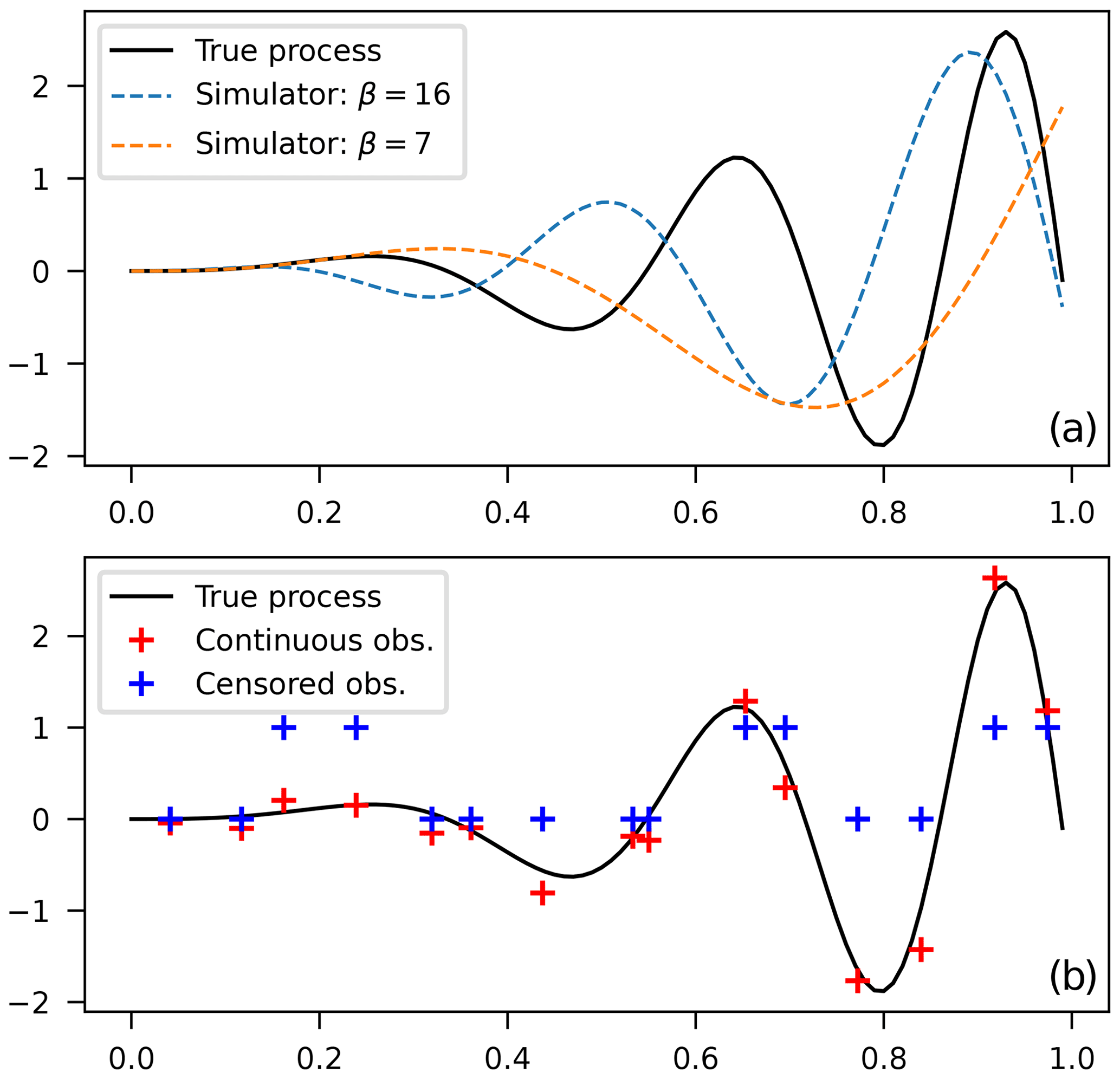
Figure 1(a) Synthetic true model and realizations of computational model runs and b) uncensored and binary observations of the true process.
In every case in this example, posterior samples of parameters were obtained by means of Markov chain Monte Carlo (MCMC) methods.
3.1 Model calibration with uncensored observations
Calibrated predictions with uncensored observations are included to have a better understanding of the limitations of having binary observations. The prediction model is the same as Model 3 defined in Sect. 2.2.3, with the difference that for uncensored observations, we have . This is in line with the standard theory of GP regression, where the simulator output S appears as a deterministic additive term, which can be found in Rasmussen and Williams (2006) and in Hall et al. (2011) applied to inundation models. The predictive distribution for new observations and the parameters' likelihood is given by Eqs. (27) and (28).
Model predictions are shown in Fig. 2 for (1) the computational model alone δ≡0, for (2) the inadequacy function alone S≡0, and for (3) the full model. It can be seen, as expected, that the simulator alone cannot reliably predict the data in the entire range since it cannot capture the varying frequency of the true process. The likelihood shows many peaks for different β values corresponding to different possible models: low-frequency where the data are fitted rather well in the left end of the range or high-frequency where the data are fitted well in the right end of the range (shown by the one plotted in Fig. 2). The narrow uncertainty bounds reflect the choice of a narrow prior to converge to one of these models. Choosing a “less informative” prior might result in unreasonably large confidence bounds and a predictive curve that mixes rather physically distinct models, rendering it useless.
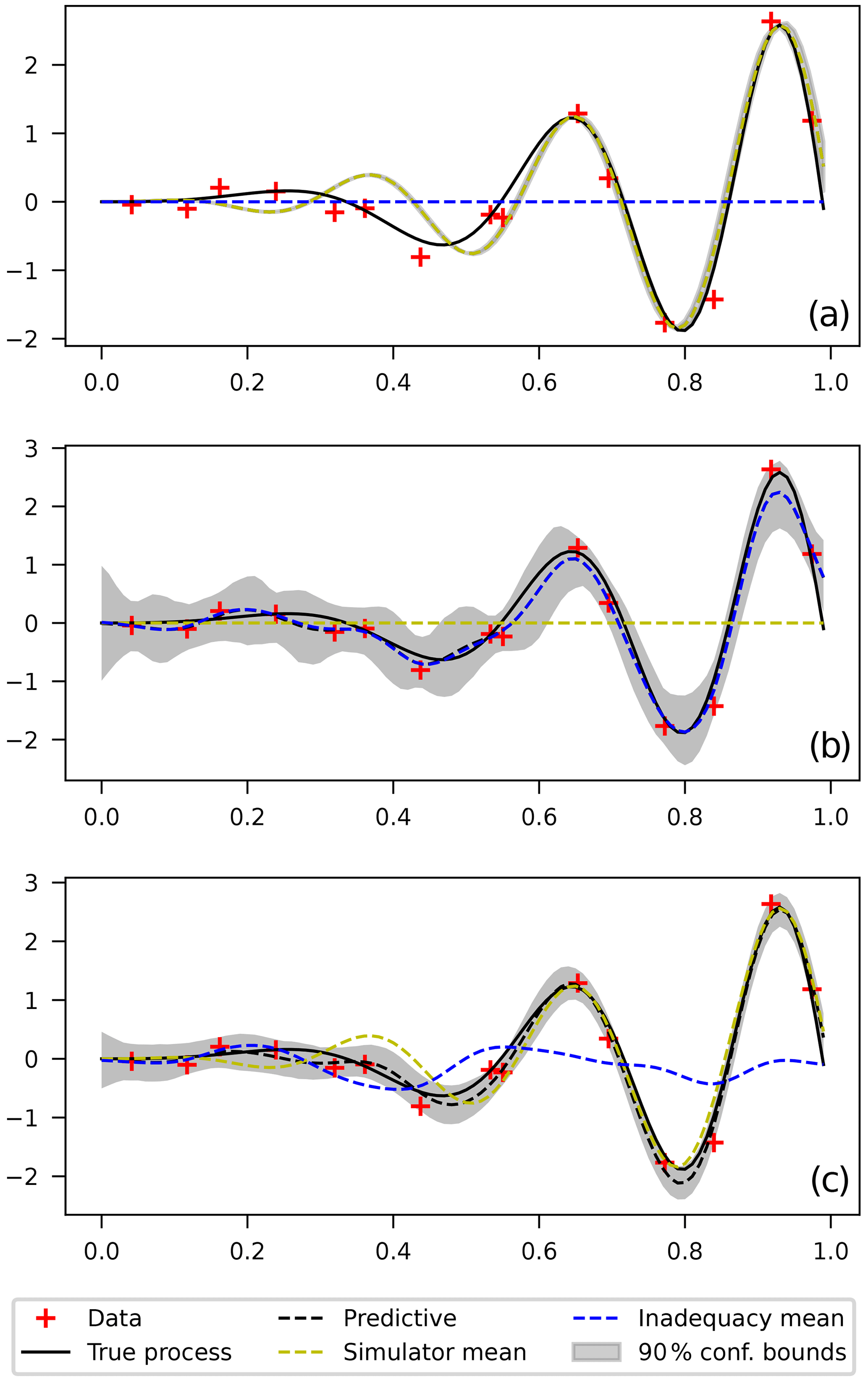
Figure 2(a) Calibration using computational model only, (b) calibration using inadequacy function only, and (c) calibration using computational model and an additive inadequacy function.
On the other hand, the middle plot shows that the flexibility of the GP prior allows the data to be fitted adequately everywhere without the need of the computational model. For the full model (lower plot), it can be seen that both the simulator and the inadequacy contribute to correctly fitting the data everywhere.
For the latter case, model parameters are, a priori, unidentifiable since the inadequacy function competes with the simulator in order to fit the data. That is, for any given set of simulator parameters β, a posterior distribution for the inadequacy parameters θ can be found that appropriately fits the data. To solve this, we fixed the values of simulator parameters β to be close to the ones obtained in the first case (see full dotted yellow line in plot) and let the inadequacy correct the predictions only where necessary (see the dotted blue line in the plot). This is in line with the suggestions in Reichert and Schuwirth (2012) and Wani et al. (2017) and is based on the assumption that physics-based computational simulators are expected to have better extrapolating capabilities to unseen events than the inadequacy function. Numerically, this is done by assigning narrow priors for β in the region where the simulator alone does a better job.
3.2 Model calibration with binary observations
In the case of binary observations, the role of the inadequacy function in data fitting becomes more complex. Using only the inadequacy to fit the binary data, the model shows a reasonable fit for the varying frequency but an approximately constant amplitude over the entire range (see Fig. 4). This reflects the limited information that binary data comprise relative to the uncensored counterpart. In particular, binary data do not give information about the amplitude of the true process, only about its crossings over the 0 axis (also termed function roughness, or frequency content).

Figure 3Log-likelihood function for the binary observations as a function of the inadequacy function parameters.
It is expected that parameters that control the “amplitude” of the inadequacy function (and/or the simulator) remain largely unidentified (Oliveira, 2000; Berrett and Calder, 2016). This is the case of the marginal variance θ1 in the squared exponential kernel of the Gaussian process. Using a very wide prior for this parameter will yield arbitrary large uncertainty bounds since data do not constrain its amplitude (i.e., the posterior is also very wide). To show this, Fig. 4 compares two calibrations using relatively wide priors for θ1 but centered at different values. Results show a similar frequency pattern but radically different amplitudes due to the different priors of θ1. In the same line, the noise parameter σ is also not identifiable since the binary operator filters out the high-frequency–low-amplitude influence of the white noise.
As a result, the amplitude of the inadequacy remains unidentified by the data but at the same time has a very significant impact on predictions: an arbitrarily large θ1 will imply arbitrarily large amplitudes of the inadequacy function, yielding physically unrealistic predictions, while very low θ1 values will yield very low amplitude for the inadequacy, rendering it virtually useless for calibration. In this context, the influence of the simulator in calibration becomes of paramount importance. It is the only component that can give a reliable assessment of the amplitude of the true process, while the inadequacy can help correct for the spatial structure (i.e., crossings over the 0 axis) wherever the simulator is deficient.
There is no strict guidance on what value to center the prior at for θ1, but a rule of thumb would indicate using the lowest value that clearly improves the fit with observations. This allows us to prioritize the simulator term in predictions as much as possible while still improving the fit to data, since the likelihood is relatively flat as a function of θ1 (as explained in the previous paragraph). This can be justified by inspection of the log-likelihood function as a function of the inadequacy parameters as shown in Fig. 3: the function is practically insensitive to θ1 for values θ1>1, indicating small information content related to that variable, and it rapidly becomes flat for lower values, indicating small information content for both variables.
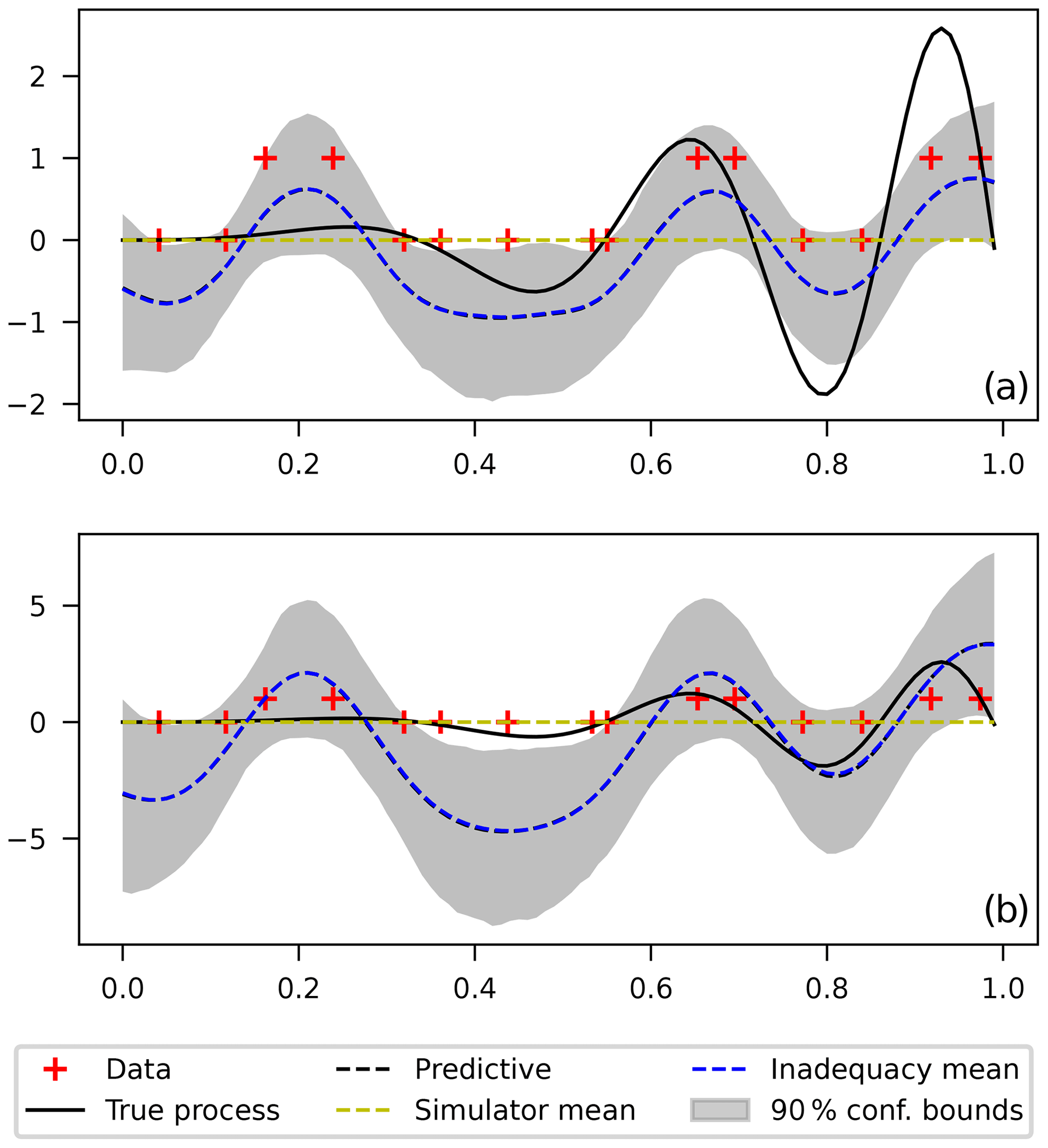
Figure 4Calibration using the inadequacy function only for a θ1 prior centered at 1 (a) and centered at 20 (b).
Figure 5 shows different calibrations using both the simulator and the inadequacy for narrow θ1 priors centered at different values. A very low value (upper plot, with a prior centered around 0.02) implies that the inadequacy practically does not modify the simulator output anywhere, while a very large value (lower plot, with a prior centered around 20) implies that the inadequacy amplitude overshadows the simulator output everywhere but specially where the simulator on its own does not fit the data correctly. A prior for θ1 centered around 0.1 seems to balance the amplitude tradeoff reasonably well (middle plot), giving significant improvement over the simulator alone but still leaving the simulator output to predominate over the inadequacy. This also reinforces the idea that the simulator should be fixed around its best values, as was explained in the uncensored data case.
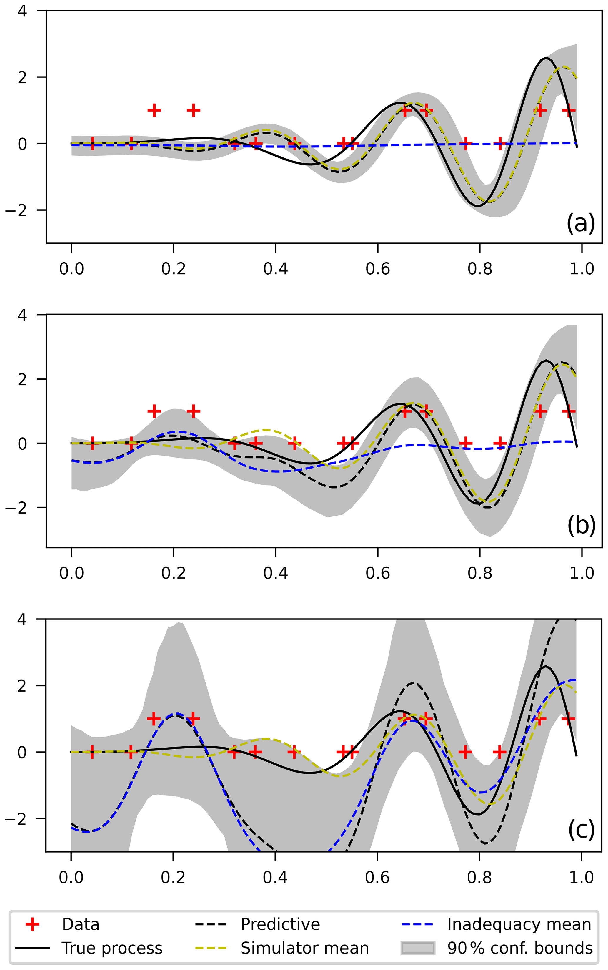
Figure 5Comparison of calibration using both the simulator and the inadequacy function for different prior means for θ1: 0.02 (a), 0.1 (b), and 20 (c).
4.1 Description and observations
The case study is based on a short reach on the upper river Thames in Oxfordshire, England, just downstream from a gauged weir at Buscot. The river, at this location, has an estimated bankfull discharge of 40 m s−3 and drains a catchment of approximately 1000 km2 (Aronica et al., 2002). The topography DEM was obtained from stereophotogrammetry at a 50 m scale with a vertical accuracy of ±25 cm, obtained from large-scale UK Environment Agency maps and surveys (see Fig. 6).
For calibration, a satellite observation of the flood extent of a 1-in-5-year event that occurred in December 1992 was used (Fig. 6). The binary image of the flood was captured 20 h after the flood peak when discharge was at a level of 73 m3 s−1 as per the hydrometric data recorded by the gauging station (Aronica et al., 2002). The resolution of the image is 50 m. As described in previous research, the short length of the reach and the broadness of the hydrograph imply that a steady-state hydraulic model is sufficiently accurate for the calibration (Aronica et al., 2002; Hall et al., 2011).
4.2 Inundation model
The computational inundation model used is the raster-based LISFLOOD-FP model (Neal et al., 2012). LISFLOOD-FP couples a 2D water flow model for the floodplain and a 1D solver for the channel flow dynamics. Its numerical structure makes it computationally efficient and suitable for the many simulations needed for probabilistic flood risk analysis and model calibration.
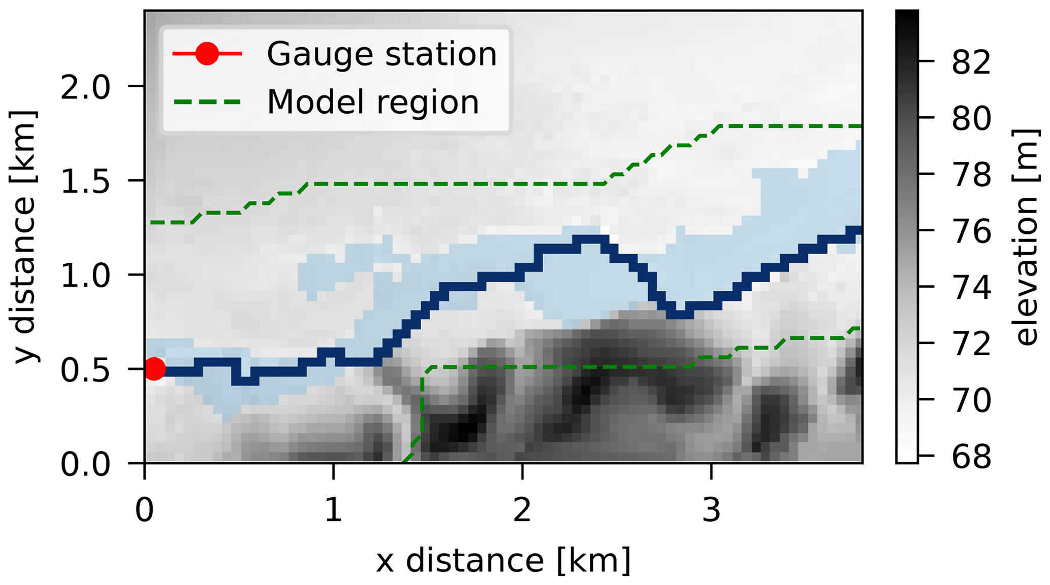
Figure 6Floodplain topography at Buscot, with SAR imagery of a 1992 flood event, channel layout, and gauge station location.
A simplified rectangular cross-section is used for the channel with a constant width of 20 m for the entire reach and a varying height of around 2 m. The observed event is defined by the boundary condition of a fixed input discharge of ν=73 m s−3 at the geographic location of the gauging station shown in Fig. 6 and by an assumed downstream boundary condition of a fixed water level of approximately 90 cm above the channel bed height. The model's parameters used for calibration are Manning's roughness parameters for the channel rch and for the floodplain rfp, both considered spatially uniform in the domain of analysis. That is, . Higher dimensionality for the simulator's parameters (e.g., spatially varying roughness) might add computational burden to an already demanding problem, and further identifiability issues could also arise.
4.3 Numerical implementation
The calibration routine was implemented in the programming language R (R Core Team, 2020) and the pmvnorm function of the TruncatedNormal (Botev and Belzile, 2021) package to compute the high-dimensional integral of the likelihood function (Eq. 18). The function rtmvnorm from the same package was used to sample from the truncated normal distribution of Eq. (23). These two evaluations were the most time-consuming of the entire process due to the high-dimensionality of the observations (around 1800 pixels): while a single run of the inundation model takes around 3 s in a 10-core Intel i9-10700K processor, one likelihood evaluation takes around 40 s. The original image of the reach was trimmed closer to the flood extent to reduce the number of observations for calibration, as seen in Fig. 6.
For models 2 and 3, both the predictive distribution of new observations and the posterior distributions of the model parameters were sampled using an adaptive MCMC scheme. A Gaussian jump distribution was used to select candidates, where the covariance matrix was empirically obtained from initial runs of the chain and subsequently scaled up and down in order to obtain an acceptance ratio of around 0.25. Two chains of 15 000 runs with an initial adaptive step of 5000 were used in order to ensure adequate mixing and stabilization of the chains, as measured by a Gelman–Rubin convergence diagnostic (Gelman et al., 2013) below 1.05. Total time for the 40 000 runs was around 2 weeks for Model 3 and around a day for Model 2.
4.4 Results
Calibrated predictions for the observed event are obtained using the three methods described in Sect. 2.2. These predictions are then compared to the satellite binary observation through the goodness-of-fit metrics in Eqs. (25) and (26). The “probability of flood” map is obtained empirically from the prediction samples, by computing the proportion of samples where each pixel is flooded as described in Sect. 2.3. This can be considered a measure of the training error as it is computed for the observed event and observed pixels.
4.4.1 Model 1: GLUE
The inundation model was run for a fine grid of β with uniform probability (prior) in the region and . Only runs with F>0.45 were retained as “behavioral” solutions for posterior analysis and prediction, with a maximum of F=0.52 obtained for rch=0.029 and rfp=0.045 (see Fig. 7). While this leaves out the large majority of the runs, visual inspection showed that values lower than F=0.45 could yield unacceptable inundation patterns. It appears form the marginal posterior distributions of Fig. 7 that the model fit is better for lower values of channel or floodplain roughness.

The probability of flood and misprediction rate ρ maps in Fig. 8 show that all accepted simulations systematically mispredict (over- or underpredict) inundation at several regions around the edge of the flood extent, yielding an average misprediction rate of P=0.08. This can be due to limitations of the LISFLOOD-FP model in capturing the spatial behavior of the true event or some spatial dependent error in the input data (e.g., DEM) or, most probably, a combination of both.

It is important to stress again that the results of the GLUE model are very sensitive to the acceptance threshold used (in this case, F>0.45). A lower threshold implies larger areas with more uncertain inundation patterns and larger areas of relatively low probability of misprediction, while retaining only a few of the best simulations (i.e., a higher threshold) yields less variability in predictions and smaller areas with a higher probability of misprediction, as in the results of Fig. 8.
4.4.2 Model 2: no inadequacy and independent observations
This model is tested with a binary-channel observation error structure (see Sect. 2.2). Since parameters β are strictly positive, and {σ1,σ2} lie in the range [0, 1], appropriate real-valued transformed variables were used for calibration through MCMC: log-transformation for the former and probit transformation for the latter. Gaussian distributions were used for the prior of the transformed variables in all cases, with a relatively wide variance to reflect non-informativeness. For the {σ1,σ2}, the prior means also reflect the fact that values above 0.5 are expected in each case (e.g., assuming that the observation error is not unrealistically large).
Prior and posterior distribution for model parameters are shown in Fig. 9. It can be seen that the posterior of the LISFLOOD-FP parameters is narrowly concentrated around fixed best-fit values: rch=0.03 and rfp=0.045. For the observation error parameters, the posteriors are narrowly concentrated around σ1=0.82 and σ2=0.98, implying that overpredictions are more “accepted” than underpredictions. The model likelihood seems to clearly discriminate this set of parameters against any other, resulting in practically no variability in predictions. This is in agreement with the results obtained by Woodhead (2007) and has to do with the shape of the likelihood function (Eq. 15), where for σ1 and σ2 values close to 1, a slight change in the number of mispredicted pixels results in a large change in the likelihood. On the other hand, values equal to 0.5 would imply a constant likelihood (see Eq. 15) and no information gained from data.
Probability of flood and misprediction rate ρ maps are shown in Fig. 10. Systematic mispredictions are observed in many places, mainly overpredictions, along the edge of the observation with a resultant average rate of P=0.072. Since this calibration results in a “single best prediction”, all mispredicted pixels result in systematic errors (i.e., for every simulation), highlighting the limitations of this spatially independent discrepancy model. Results are very similar to the GLUE model with a very high threshold (only keeping a single “best” run).
4.4.3 Model 3: inadequacy function and independent observations
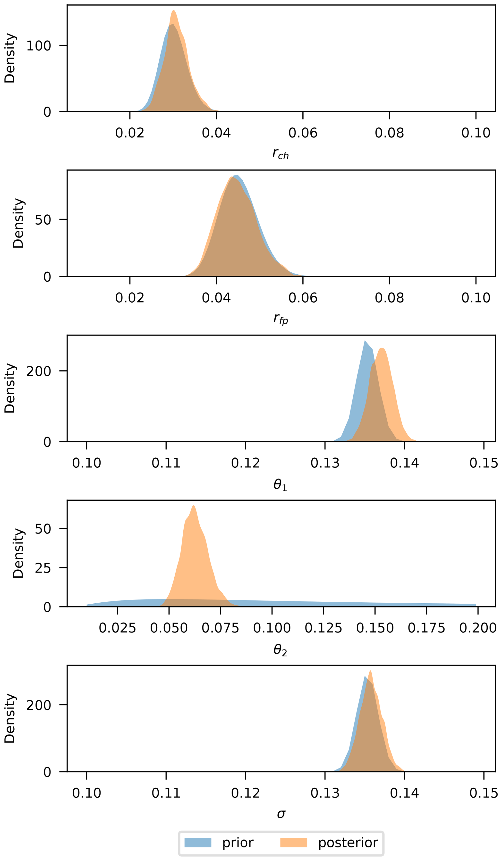
Model 3 was run with narrow priors for the simulator parameters centered around the best values obtained in the previous independent model. As explained in Sect. 3, this was done to avoid identifiability problems with θ1, letting the simulator “do its best” while only using the inadequacy term where necessary. Narrow priors were used, both centered at 0.1, to keep the amplitude of the inadequacy function relatively low (but not too low, as discussed in Sect. 3). The parameter θ2 that prescribes the spatial frequency (i.e., crossings over the 0 axis) of the inadequacy function was calibrated using a Gaussian non-informative prior centered around 0.14. In every case, calibration was done for the logarithm of the parameters to preserve their positiveness.
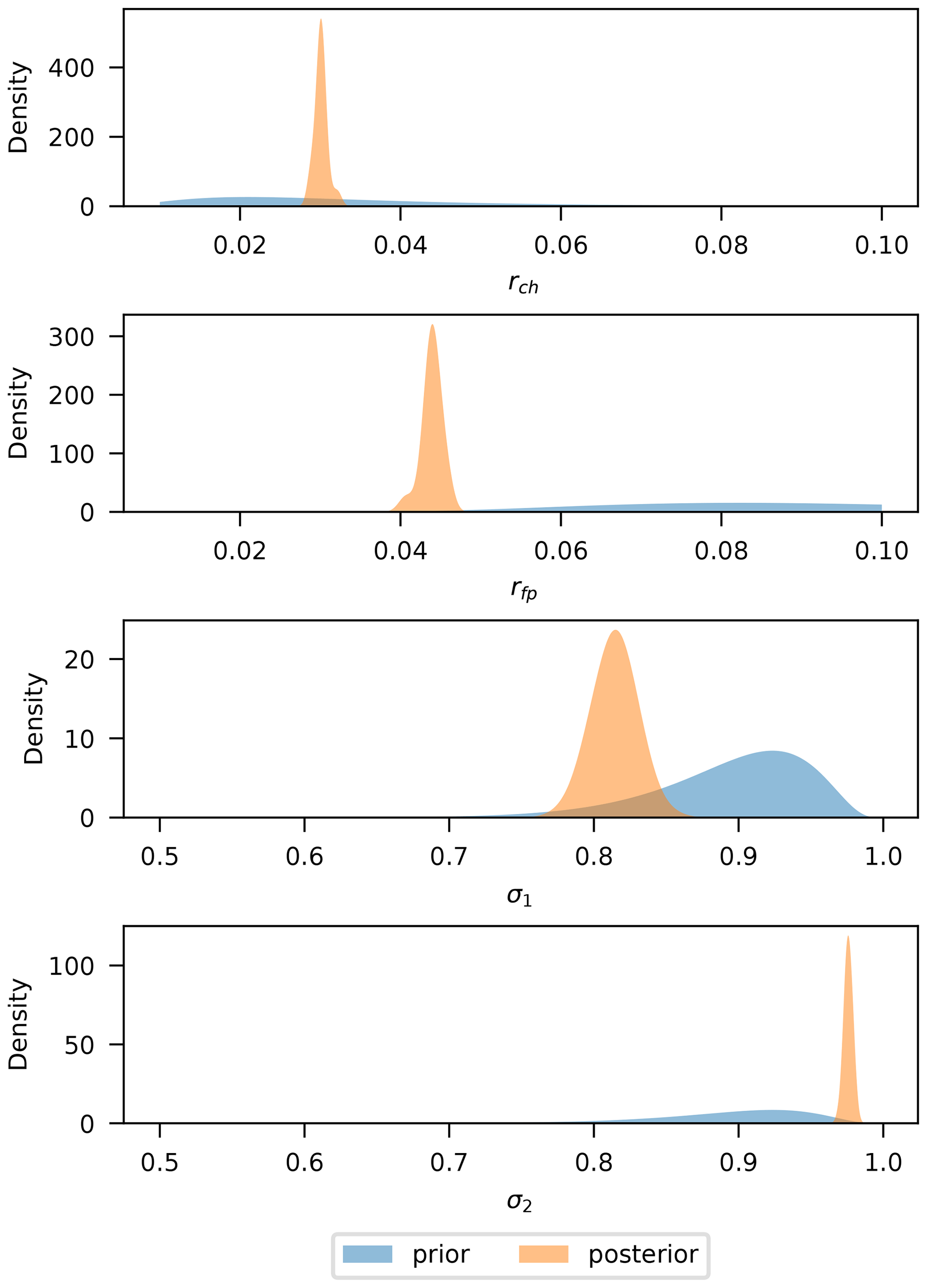
Prior and posterior distributions of the transformed parameters are shown in Fig. 11. The posteriors of the simulator parameters (upper plot) are distributed very close to their priors as intended. The same goes for θ1 and σ, where the posteriors have the same width as the priors. The roughness parameter θ2, on the other hand, contains most of the information gain from observations in this model, as can be seen from the very narrow posterior distribution as compared to the vague prior. This is expected, as explained in the illustrative example of Sect. 3, since it is the only parameter from the kernel that can gather meaningful information from binary data.
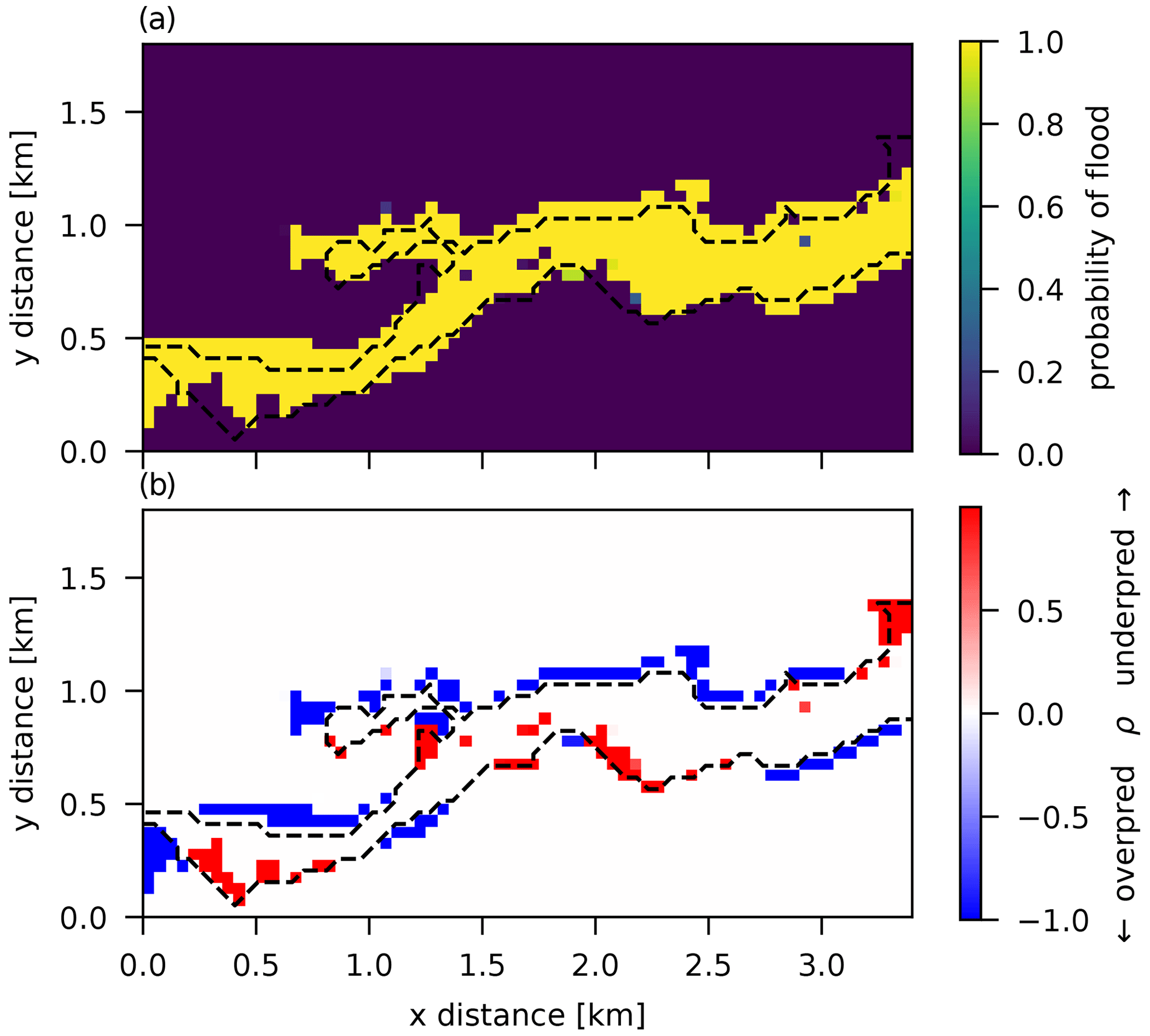
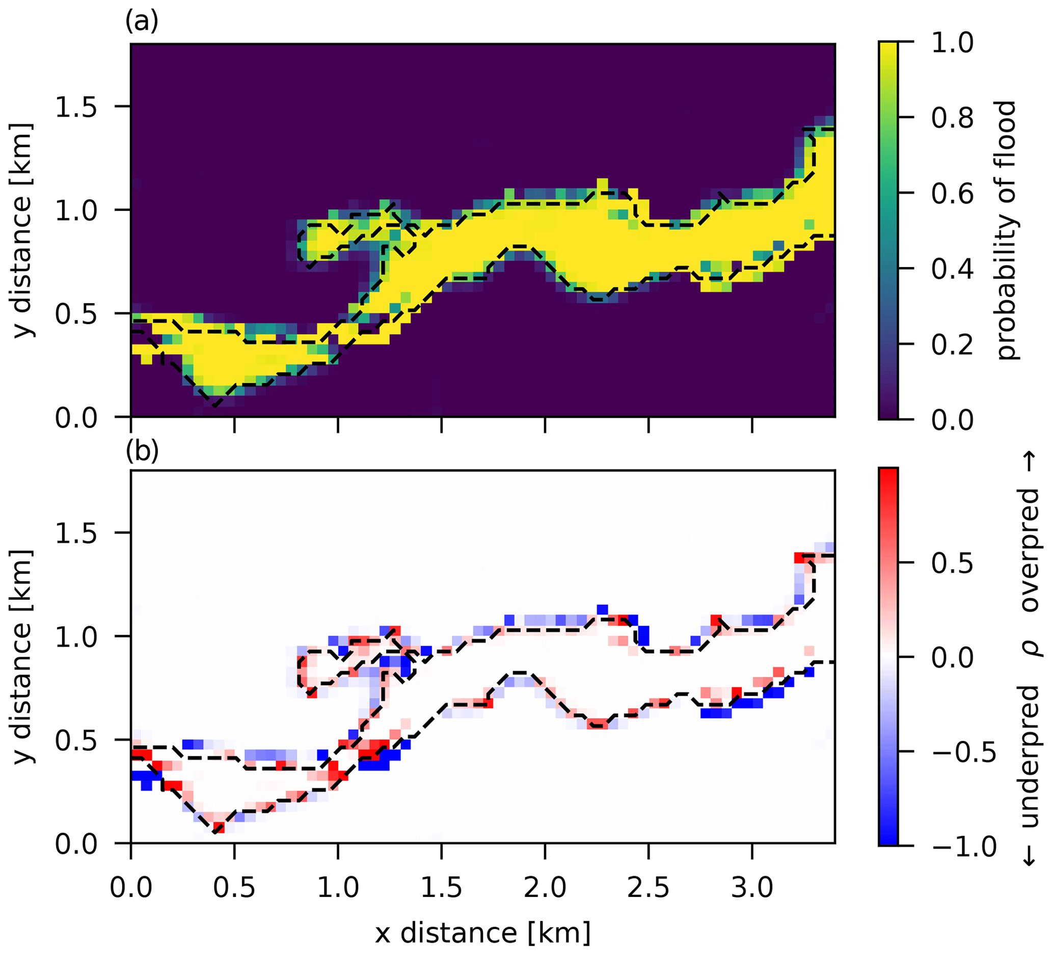
Probability of flood and misprediction rate ρ maps are shown in Fig. 12. It can be seen that the inadequacy function deals with many of the systematic misprediction regions that the simulator had when used alone for prediction, as in the previous two models. This model yields an average misprediction rate of P=0.057 and also displays a different spatial pattern where over- and underpredicted pixels seem to be more uniformly distributed along the observed flood extent edge.
The methodology and results shown in the previous sections indicate that satellite-borne binary observations can provide valuable information for inundation model calibration and that explicitly modeling the spatially correlated discrepancy between the simulator output and observations through an inadequacy term can improve predictions. In this section we discuss some of the main takeaways from the results obtained for the illustrative example and the real-world case study.
5.1 Model building and hypothesis
The traditionally used GLUE framework was described and compared to a more general and formal framework in which appropriate probabilistic models were assigned to the discrepancy between observations and simulator output. The main advantages of this methodology are (1) the capability of consistently including the different sources that add to the discrepancy such as observation errors or simulator inadequacy and (2) the computation of formal probability distributions, and thus uncertainty bounds, for readily observed or future events. This does not mean that any calibrated predictions and uncertainty bounds within this formal framework are “better” than another obtained by GLUE, but it does have the potential for a more transparent and flexible model setup that can include all the modeler's prior knowledge and observations consistently.
A basic assumption that was used for model building here is that observation errors are spatially independent and homogeneous (identically distributed). Model 2 was a simple model built by assuming that all of the discrepancy between observations and the simulator output could be explained by this type of observation error alone. Results from this model, and from GLUE (see Figs. 8 and 10), show that the discrepancy is spatially correlated, reflected by regions of systematically under- or over-flooded pixels, indicating that the simulator on its own cannot capture the spatial structure of the observed extent everywhere. This could be due to a more complex observation error structure (uncertainty in satellite image acquisition and interpretation), due to limitations in the physical representation given by the equations in the model or due to errors in the boundary conditions (e.g., error in the DEM used). Most probably, it is a combination of all.
These results also highlight the importance of explicitly modeling the spatial correlation that is not captured by the computational simulator. Model 3 implements this through an additive inadequacy term with a spatially correlated Gaussian process prior. Implicit in this model is the fact that all spatial correlation in discrepancy is assigned to simulator inadequacy and none to the observation errors (assumed independent). This, of course, could be challenged in the light of further information or knowledge, as in the error models studied by Woodhead (2007), but it remains a common assumption in the calibration of physical models (Kennedy and O'Hagan, 2001).
5.2 Uncertainty quantification
The plots in Fig. 13 show the predictive distribution of flood depths for three different points observed flooded for the three calibration models. The GLUE model results reflect an uncertainty in line with the wide posteriors obtained for the simulator roughness parameters. These are, however, highly dependent on the threshold value used and what the modeler considers to be a behavioral model.
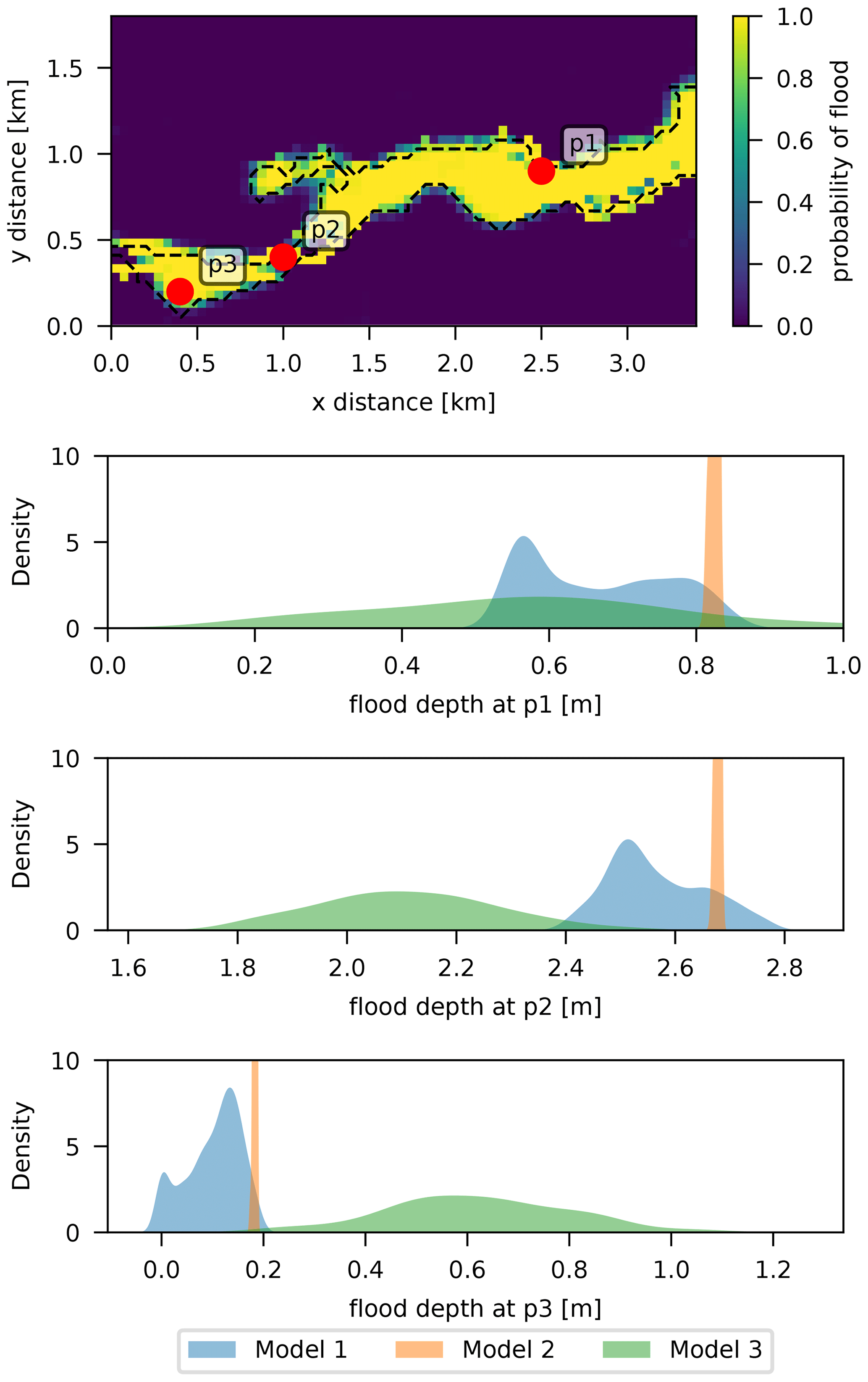
Figure 13Predictive distributions of flood depths for three different points in the floodplain.
On the other hand, Model 2 predictions are practically deterministic since no uncertainty is reflected in the posterior predictions. This might be an indicator of the model's inability of representing the true process rather than goodness-of-fit, as seen from the spatially correlated regions of under- and overpredicted pixels in Fig. 10 and the larger misprediction rate of this model compared to Model 3. However, assuming a larger observation error by fixing values of σ1 and σ2 closer to 0.5 could allow for a larger, more realistic uncertainty in the flood depths obtained, similar to the influence that the threshold value has in the GLUE model.
Finally, Model 3 shows larger uncertainty in predictions that is contributed entirely by the inadequacy term, since the simulator parameters have a very narrow posterior. The wider shape of the distributions is also in line with the results shown for the 1D-illustrative example. The predictive distributions can also be shifted from the ones obtained by GLUE or Model 2, due to the addition of the inadequacy term to the simulator. These aspects are discussed in the subsequent sections.
It is important to state again that a better or more reliable likelihood does not imply smaller uncertainty bounds but rather a more consistent way of dealing with the different sources of uncertainty. In this case, as shown in the illustrative example, not considering spatial correlation of residual (as in Model 2) can yield unrealistically optimistic uncertainty bounds; the same would happen if using a very high threshold in GLUE.
5.3 Role of the inadequacy function
As explained before, results from the GLUE model indicate that the discrepancy between observed flood extent and simulator output is spatially dependent. That is, there are areas where the simulator systematically underpredicts or overpredicts flooding. The additive inadequacy term in Model 3 takes the role of modeling this spatial dependence of simulator deficiencies, since the observation error term is considered independent in all models. It can reflect inaccuracies in the input spatial data, such as DEM, channel depth or width, and roughness parameters, or structural deficiencies of the mathematical simplifications of the simulator.

Figure 14Flood-depth maps from Model 3 predictions of the simulator and inadequacy (a, b), the simulator alone (c, d), and inadequacy (e, f) for a marginal prior mode of θ1=0.05 (a, c, e) and θ1=1 (b, d, f). The dashed black line is the observed flooded extent.
Adding the inadequacy function better replicates the observed inundation extent, but it can also distort the depths at the flooded pixels if its values are not restricted, yielding unrealistic patterns (see discussion in Sect. 3). These local distortions are expected to have a lesser influence than the simulator's inherent deficiencies if kept constrained at reasonable levels. A very low value for the inadequacy amplitude, on the other hand, would result in virtually no improvement in the goodness-of-fit of calibrated predictions and the observed extent. This can also be seen in the predictive distributions of Fig. 13, where they can be shifted relative to the other models that only use the simulator for prediction.
The plots in Fig. 14 show a comparison of a single flood-depth prediction (zoomed in at the bottom left corner of the extent) using the posterior mode parameters, for the simulator alone (middle), the simulator and the inadequacy (upper), and the inadequacy (lower) for a marginal variance prior centered at θ1=0.05 and θ1=1. As expected, it can be seen that the inadequacy is positive where the simulator tends to underpredict and negative where it tends to overpredict. However, it is not 0 for the correctly predicted pixels, and this is added to the simulator output. This distortion is much larger for the larger marginal variance θ1, as can be seen in the right-column plots (and consistent with the synthetic results from Fig. 5), with up to 2 m of flood depth added in some correctly predicted pixels due to the inadequacy term. The predicted overall flood extent (and, thus, the fit to the observations) is very similar in both cases.
As mentioned at the beginning of this section, the inadequacy term can represent complex spatial (and eventually temporal) error structures from input data and simplified process representations. It enables the construction of improved simulations by combining the explanatory and extrapolating capabilities of physics-based models with the optimized prediction of statistical models. Results from the synthetic example in Sect. 3 suggest that this symbiosis requires expertise in constraining the inferential process of the physics-based model to realistic values. This is relevant for a very broad range of applications that go beyond the inundation case study developed in this work (see Sargsyan et al., 2015; Wani et al., 2017; Cao et al., 2018; Chang et al., 2019), where simplified process representations are required in order to perform robust uncertainty analysis.
5.4 Information content of binary observations
The illustrative 1D example in Sect. 3 was specifically selected to show the limitations that using censored observations imply for predictive accuracy, model building, and numerical modeling. Censored binary observations, as explained, do not provide information about the magnitude of the true process output (i.e., flood depths) but only about its spatial frequency (i.e., crossing over the 0 axis). This means that when only censored observations are available, an appropriate simulator is of paramount importance to obtain meaningful predictions, as is seen in Fig. 5.
From a numerical standpoint, binary observations do not provide information about the marginal variance θ1 that controls the inadequacy amplitude. To avoid identifiability and convergence problems, a narrow prior (or simply fixing the value) is required, centered at an appropriate value following the criteria mentioned previously: not too large to unrealistically distort simulator outputs but large enough to improve fit to the observations where needed. For this reason, relatively large uncertainty bounds on flood-depth predictions are also expected, as can be seen from Figs. 5 and 13.
The noise parameter σ also remains mostly unidentifiable since it is filtered out by the censoring, and it does not seem to significantly affect the results if kept within reasonable values (similar to the θ1 magnitude for this case study). Further experiments are needed to analyze the influence and tradeoffs of the marginal variance and noise values used in calibration.
5.5 Limitations
As explained in the Introduction, the main reason for the popularity of GLUE models is its conceptual simplicity and ease of implementation. This is, at the same time, a limitation of the proposed Bayesian model. The discrepancy between a simulator output and observations of the real process can be very complex and non-stationary (both in space and time).
Due to its flexibility and well-known analytical properties, GPs are a good choice to predict complex and correlated residual structures but also carry the risk of over-fitting observations. When uncensored data are available, this can be controlled with an appropriate level of observation noise (e.g., σ in our framework). When only binary data are available, however, noise is not distinguishable in the likelihood, and over-fitting can pose a serious problem. Our proposed approach to deal with this is to give the simulator a predominant role in prediction while restricting the inadequacy “only where necessary”. This implies verifying improvements in the fit of the model in those places where the simulator alone systematically mispredicts and also checking the absolute values of predictions to prevent unrealistic values from the inadequacy function. This, still, requires modeler expertise and knowledge about the particular problem at hand.
In the same line, an implicit hypothesis of the model is that the inadequacy function does not depend on the forcing event ν. This was assumed more from data availability than from theoretical grounds. While a single event might be informative of the inadequacy function, particularly if deficiencies in the simulator are due to input errors (e.g., DEM inaccuracies), it is also expected that some of the simulator deficiencies in predicting the true process are dependent on the magnitude of the events being predicted. This issue could be approached by calibration with observations from events of different magnitude, resulting, of course, in higher computational demand.
In this regard, an important limitation of the proposed Bayesian model with spatially correlated inadequacy function is the computational burden. While this is also a limitation for any calibration method, in this case, the likelihood function (Eq. 18) is very time-consuming with current computational capacities and mathematical techniques (Genz, 1992), even for a small reach like the one studied here. The same goes for sampling from the truncated normal in Eq. (23) for calibrated predictions. Widespread adoption of this formal model, thus, requires the elaboration of more efficient techniques for computing and sampling from very high dimensional Gaussian distributions or studying ways of using less observations without losing important information. Dimensionality reduction techniques are expected to play a role in this favor (Chang et al., 2019).
Efficient management of risk due to hazards requires reliable predictions of very complex physical processes, such as inundations. Hence, it is important to have adequate predictive models that can capture the relevant spatial features of flooding, making use of all available real-world data. This paper proposes a fully probabilistic framework for the statistical calibration of inundation simulators using binary observations of flood extent, such as the ones obtained from satellite observations and publicly available worldwide. Probabilistic inferences for new flood events can then be coupled with frequency models (also Bayesian) to obtain reliable and robust probabilistic inferences of flood hazard (and eventually flood damage). Furthermore, the framework's capability of explicitly modeling the structure of the observation errors and simulator deficiencies paves the way for the consistent inclusion of data from different sources (e.g., satellite-borne, ground depth measurements, crowdsourced) in future works.
The newly proposed model, which can explicitly model the simulator structural deficiencies through an inadequacy term, is used in a real case study, and the results are compared to the traditionally used GLUE framework and to a simpler Bayesian model without the inadequacy term. Results show that calibrated predictions done for models without the inadequacy function and independent observation errors show systematic mispredictions in certain regions of the flood extent, reflecting that the likelihood functions used (or pseudo-likelihood in the case of GLUE) do not capture the spatial complexity of the observations. Including the inadequacy term, acknowledging the spatial correlation of the simulator's discrepancy with observations, can help improve predictions as measured by a lower average misprediction rate (from 0.072 to 0.057) and by removing regions with systematic errors in predictions.
We show that an appropriate physics-based simulator is needed to obtain meaningful inferences when only binary (i.e., censored) observations are available. The inadequacy function and the simulator compete with each other to fit the data, and we suggest that it is reasonable to let the simulator do “as best as it can” and the inadequacy function correct only where necessary. This is due to better extrapolating capabilities of the physics-based models but also because censored observations do not carry information about amplitudes (i.e., water depths) of the true process. Resulting predictions can be very sensitive to the priors used, in the same way GLUE results are extremely sensitive to the threshold use to discriminate behavioral models.
From a numerical implementation standpoint, the proposed model proves to be computationally intensive, and care must be taken in the definition of the model hyperparameters to avoid identifiability and convergence problems. Further work remains to be done, particularly by implementing more efficient numerical techniques for computing high-dimensional integrals and/or exploring ad hoc ways of reducing the computational burden of the likelihood function (e.g., leaving out neighboring pixels).
As stated before, the main benefit of the proposed model lies in the explicit and disaggregated modeling of the different sources of uncertainty, such as observation errors and simulator inadequacy. The inadequacy term allows us to account for structural deficiencies in the physics-based simulator used and/or undetected errors in input information (e.g., DEM). Furthermore, different data sources could be consistently combined for inference within the same framework by simply considering different observation error structures (e.g., as in Eqs. 4 and 3). This is particularly useful when combining observations from very different sources such as satellites, crowdsourcing, or ground sensors: they all might have different observation error structures ε, but the inadequacy term that is part of the true process should remain the same for all.
In this light, it would be interesting to develop illustrative examples, as well as real case studies, where censored (satellite radar data) and uncensored data (ground flood height measurements) are available. This could exploit and combine the capacity of uncensored observations in constraining uncertainty in the model's predictions (Werner et al., 2005) and the spatially distributed availability of satellite data.
All data used in this paper are publicly available. All the data (including satellite observations and LISFLOOD-FP input files) and source codes used in this paper are available at https://doi.org/10.5281/zenodo.7682138 (Balbi, 2022).
The paper was written by MB. MB built the mathematical models, compiled the data, and performed the analysis. DCBL gave critical feedback at all stages of the research process and all sections of this paper.
The contact author has declared that neither of the authors has any competing interests.
Publisher's note: Copernicus Publications remains neutral with regard to jurisdictional claims in published maps and institutional affiliations.
Jim W. Hall, from Oxford University, is thanked for freely providing the satellite observation for the 1992 flood event at the reach under study. Paul Bates and the LISFLOOD-FP development team are thanked for their support during the simulator learning curve and for the free access to their software, including manuals and tutorial examples, which this case study was drawn from.
All of the work was performed in publicly available and free languages (Python and R) and software (LISFLOOD-FP). The authors thank the open-source community for its invaluable contribution to science.
The research was partially funded by the School of Engineering of the University of Buenos Aires, Argentina, through a Peruilh doctoral scholarship. This research was also supported by the Ministry of Education, Singapore, under its MOE AcRF Tier 3 award.
This research has been supported by the Ministry of Education, Singapore (grant no. MOE 2019-T3-1-004) and Earth Observatory of Singapore contribution number 516.
This paper was edited by Micha Werner and reviewed by two anonymous referees.
Alfonso, L., Mukolwe, M. M., and Di Baldassarre, G.: Probabilistic Flood Maps to Support Decision-Making: Mapping the Value of Information: Probabilistic Flood Maps To Support Decision-Making: VOI-MAP, Water Resour. Res., 52, 1026–1043, https://doi.org/10.1002/2015WR017378, 2016. a
Aronica, G., Bates, P. D., and Horritt, M. S.: Assessing the Uncertainty in Distributed Model Predictions Using Observed Binary Pattern Information within GLUE, Hydrol. Process., 16, 2001–2016, https://doi.org/10.1002/hyp.398, 2002. a, b, c, d, e, f, g
Balbi, M.: Code and Data Github repository for “Bayesian calibration of a flood simulator using binary flood extent observations”, Zenodo [code and data set], https://doi.org/10.5281/zenodo.7682138, 2022. a
Bates, P. D., Horritt, M. S., Aronica, G., and Beven, K.: Bayesian Updating of Flood Inundation Likelihoods Conditioned on Flood Extent Data, Hydrol. Process., 18, 3347–3370, https://doi.org/10.1002/hyp.1499, 2004. a
Berrett, C. and Calder, C. A.: Bayesian Spatial Binary Classification, Spat. Stat., 16, 72–102, https://doi.org/10.1016/j.spasta.2016.01.004, 2016. a, b
Beven, K.: A Framework for Uncertainty Analysis, Imperial College Press, 39–59, https://doi.org/10.1142/9781848162716_0003, 2014a. a, b
Beven, K.: The GLUE Methodology for Model Calibration with Uncertainty, Imperial College Press, 87–97, https://doi.org/10.1142/9781848162716_0006, 2014b. a, b
Beven, K.: Facets of Uncertainty: Epistemic Uncertainty, Non-Stationarity, Likelihood, Hypothesis Testing, and Communication, Hydrolog. Sci. J., 61, 1652–1665, https://doi.org/10.1080/02626667.2015.1031761, 2016. a
Beven, K. and Binley, A.: The Future of Distributed Models: Model Calibration and Uncertainty Prediction, Hydrol. Process., 6, 279–298, https://doi.org/10.1002/hyp.3360060305, 1992. a
Botev, Z. and Belzile, L.: TruncatedNormal: Truncated Multivariate Normal and Student Distributions, r package version 2.2.2, https://CRAN.R-project.org/package=TruncatedNormal (last access: 5 August 2022), 2021. a
Cao, F., Ba, S., Brenneman, W. A., and Joseph, V. R.: Model Calibration With Censored Data, Technometrics, 60, 255–262, https://doi.org/10.1080/00401706.2017.1345704, 2018. a, b, c
Carbajal, J. P., Leitão, J. P., Albert, C., and Rieckermann, J.: Appraisal of Data-Driven and Mechanistic Emulators of Nonlinear Simulators: The Case of Hydrodynamic Urban Drainage Models, Environ. Model. Softw., 92, 17–27, https://doi.org/10.1016/j.envsoft.2017.02.006, 2017. a
Chang, W., Konomi, B. A., Karagiannis, G., Guan, Y., and Haran, M.: Ice Model Calibration Using Semi-Continuous Spatial Data, arXiv [preprint], arXiv:1907.13554 [stat], https://doi.org/10.48550/arXiv.1907.13554, 2019. a, b, c, d
Chib, S. and Greenberg, E.: Analysis of Multivariate Probit Models, Analysis of multivariate probit models, Biometrika, 85, 347–361, 1998. a
Di Baldassarre, G.: Floods in a Changing Climate: Inundation Modelling, in: no. 3 in International Hydrology Series, Cambridge University Press, ISBN 978-1-139-08841-1, 2012. a
Di Baldassarre, G., Schumann, G., and Bates, P. D.: A Technique for the Calibration of Hydraulic Models Using Uncertain Satellite Observations of Flood Extent, J. Hydrol., 367, 276–282, https://doi.org/10.1016/j.jhydrol.2009.01.020, 2009. a
Di Baldassarre, G., Schumann, G., Bates, P. D., Freer, J. E., and Beven, K. J.: Flood-Plain Mapping: A Critical Discussion of Deterministic and Probabilistic Approaches, Hydrolog. Sci. J., 55, 364–376, https://doi.org/10.1080/02626661003683389, 2010. a, b
Gelman, A., Carlin, J. B., Stern, H. S., Dunson, D. B., Vehtari, A., and Rubin, D. B.: Bayesian Data Analysis, in: 3rd Edn., CRC Press, ISBN 978-1-4398-4095-5, 2013. a, b, c
Genz, A.: Numerical Computation of Multivariate Normal Probabilities, J. Comput. Graph. Stat. 1, 141–149, https://doi.org/10.2307/1390838, 1992. a, b
Global Facility for Disaster Reduction and Recovery: Understanding Risk in an Evolving World: Emerging Best Practices in Natural Disaster Risk Assessment, Tech. rep., The World Bank, https://www.gfdrr.org/sites/default/files/publication/Understanding_Risk-Web_Version-rev_1.8.0.pdf (last access: 5 August 2022), 2014. a
Goldstein, M. and Rougier, J.: Probabilistic Formulations for Transferring Inferences from Mathematical Models to Physical Systems, SIAM J. Scient. Comput., 26, 467–487, https://doi.org/10.1137/S106482750342670X, 2004. a, b, c, d, e
Hall, J. and Solomatine, D.: A Framework for Uncertainty Analysis in Flood Risk Management Decisions, Int. J. River Basin Manage., 6, 85–98, https://doi.org/10.1080/15715124.2008.9635339, 2008. a
Hall, J. W., Manning, L. J., and Hankin, R. K.: Bayesian Calibration of a Flood Inundation Model Using Spatial Data, Water Resour. Res., 47, 5529, https://doi.org/10.1029/2009WR008541, 2011. a, b, c, d
Horritt, M. S.: A Methodology for the Validation of Uncertain Flood Inundation Models, J. Hydrol., 326, 153–165, https://doi.org/10.1016/j.jhydrol.2005.10.027, 2006. a, b
Hunter, N. M., Bates, P. D., Horritt, M. S., De Roo, A. P. J., and Werner, M. G. F.: Utility of Different Data Types for Calibrating Flood Inundation Models within a GLUE Framework, Hydrol. Earth Syst. Sci., 9, 412–430, https://doi.org/10.5194/hess-9-412-2005, 2005. a, b, c, d
Jha, A. K., Bloch, R., and Lamond, J.: Cities and Flooding: A Guide to Integrated Urban Flood Risk Management for the 21st Century, The World Bank, https://doi.org/10.1596/978-0-8213-8866-2, 2012. a
Jiang, P., Zhou, Q., and Shao, X.: Surrogate Model-Based Engineering Design and Optimization, in: Springer Tracts in Mechanical Engineering, Springer Singapore, Singapore, https://doi.org/10.1007/978-981-15-0731-1, 2020. a
Kennedy, M. C. and O'Hagan, A.: Bayesian Calibration of Computer Models, J. Roy. Stat. Soc. Ser. B, 63, 425–464, https://doi.org/10.1111/1467-9868.00294, 2001. a, b, c, d, e, f, g, h, i, j, k
Kiczko, A., Romanowicz, R. J., Osuch, M., and Karamuz, E.: Maximising the Usefulness of Flood Risk Assessment for the River Vistula in Warsaw, Nat. Hazards Earth Syst. Sci., 13, 3443–3455, https://doi.org/10.5194/nhess-13-3443-2013, 2013. a
Mason, D. C., Bates, P. D., and Dall' Amico, J. T.: Calibration of Uncertain Flood Inundation Models Using Remotely Sensed Water Levels, J. Hydrol., 368, 224–236, https://doi.org/10.1016/j.jhydrol.2009.02.034, 2009. a
Moges, E., Demissie, Y., Larsen, L., and Yassin, F.: Review: Sources of Hydrological Model Uncertainties and Advances in Their Analysis, Water, 13, 28, https://doi.org/10.3390/w13010028, 2021. a
Neal, J., Schumann, G., and Bates, P.: A Subgrid Channel Model for Simulating River Hydraulics and Floodplain Inundation over Large and Data Sparse Areas, Water Resour. Res., 48, 1–16, https://doi.org/10.1029/2012WR012514, 2012. a
Oliveira, V. D.: Bayesian Prediction of Clipped Gaussian Random Fields, Comput. Stat. Data Anal., 34, 299–314, https://doi.org/10.1016/S0167-9473(99)00103-6, 2000. a, b, c
Papaioannou, G., Vasiliades, L., Loukas, A., and Aronica, G. T.: Probabilistic Flood Inundation Mapping at Ungauged Streams Due to Roughness Coefficient Uncertainty in Hydraulic Modelling, Adv. Geosci., 44, 23–34, https://doi.org/10.5194/adgeo-44-23-2017, 2017. a
Pappenberger, F., Beven, K., Horritt, M., and Blazkova, S.: Uncertainty in the Calibration of Effective Roughness Parameters in HEC-RAS Using Inundation and Downstream Level Observations, J. Hydrol., 302, 46–69, https://doi.org/10.1016/j.jhydrol.2004.06.036, 2005. a
Rasmussen, C. E. and Williams, C. K. I.: Gaussian Processes for Machine Learning, Adaptive Computation and Machine Learning, MIT Press, Cambridge, Massachusetts, ISBN 978-0-262-18253-9, 2006. a, b, c, d, e, f
R Core Team: R: A Language and Environment for Statistical Computing, R Foundation for Statistical Computing, Vienna, Austria, https://www.R-project.org/ (last access: 5 August 2022), 2020. a
Reichert, P. and Schuwirth, N.: Linking Statistical Bias Description to Multiobjective Model Calibration, Water Resour. Res., 48, W09543, https://doi.org/10.1029/2011WR011391, 2012. a
Romanowicz, R. and Beven, K.: Estimation of Flood Inundation Probabilities as Conditioned on Event Inundation Maps, Water Resour. Res., 39, 1073, https://doi.org/10.1029/2001WR001056, 2003. a
Romanowicz, R. J. and Kiczko, A.: An Event Simulation Approach to the Assessment of Flood Level Frequencies: Risk Maps for the Warsaw Reach of the River Vistula: Event Simulation Approach to Flood Risk Assessment, Hydrol. Process., 30, 2451–2462, https://doi.org/10.1002/hyp.10857, 2016. a
Romanowicz, R. J., Beven, K. J., and Tawn, J. A.: Bayesian Calibration of Flood Inundation Models, in: Floodplain Processes, John Wiley & Sons, ISBN 978-0-471-96679-1, 1996. a
Rougier, J.: Formal Bayes Methods for Model Calibration with Uncertainty, Imperial College Press, 68–86, https://doi.org/10.1142/9781848162716_0005, 2014. a, b, c, d
Sadegh, M. and Vrugt, J. A.: Bridging the Gap between GLUE and Formal Statistical Approaches: Approximate Bayesian Computation, Hydrol. Earth Syst. Sci., 17, 4831–4850, https://doi.org/10.5194/hess-17-4831-2013, 2013. a, b, c
Sargsyan, K., Najm, H. N., and Ghanem, R.: On the Statistical Calibration of Physical Models, Int. J. Chem. Kinet., 47, 246–276, https://doi.org/10.1002/kin.20906, 2015. a
Schabenberger, O. and Gotway, C. A.: Statistical Methods for Spatial Data Analysis, Taylor and Francis, CRC Press, ISBN 978-1-58488-322-7, 2005. a, b
Stedinger, J. R., Vogel, R. M., Lee, S. U., and Batchelder, R.: Appraisal of the generalized likelihood uncertainty estimation (GLUE) method, Water Resour. Res., 44, W00B06, https://doi.org/10.1029/2008WR006822, 2008. a, b
Stephens, E. and Bates, P.: Assessing the Reliability of Probabilistic Flood Inundation Model Predictions, Hydrol. Process., 29, 4264–4283, https://doi.org/10.1002/hyp.10451, 2015. a, b, c
Vrugt, J. A., ter Braak, C. J., Gupta, H. V., and Robinson, B. A.: Equifinality of Formal (DREAM) and Informal (GLUE) Bayesian Approaches in Hydrologic Modeling?, Stoch. Environ. Res. Risk A., 23, 1011–1026, https://doi.org/10.1007/s00477-008-0274-y, 2009. a
Wani, O., Scheidegger, A., Carbajal, J. P., Rieckermann, J., and Blumensaat, F.: Parameter Estimation of Hydrologic Models Using a Likelihood Function for Censored and Binary Observations, Water Res., 121, 290–301, https://doi.org/10.1016/j.watres.2017.05.038, 2017. a, b, c, d
Wani, O., Scheidegger, A., Cecinati, F., Espadas, G., and Rieckermann, J.: Exploring a Copula-Based Alternative to Additive Error Models for Non-Negative and Autocorrelated Time Series in Hydrology, J. Hydrol., 575, 1031–1040, https://doi.org/10.1016/j.jhydrol.2019.06.006, 2019. a
Werner, M., Blazkova, S., and Petr, J.: Spatially Distributed Observations in Constraining Inundation Modelling Uncertainties, Hydrol. Process., 19, 3081–3096, https://doi.org/10.1002/hyp.5833, 2005. a, b, c, d
Wood, M., Hostache, R., Neal, J., Wagener, T., Giustarini, L., Chini, M., Corato, G., Matgen, P., and Bates, P.: Calibration of Channel Depth and Friction Parameters in the LISFLOOD-FP Hydraulic Model Using Medium-Resolution SAR Data and Identifiability Techniques, Hydrol. Earth Syst. Sci. 20, 4983–4997, https://doi.org/10.5194/hess-20-4983-2016, 2016. a, b
Woodhead, S. P. B.: Bayesian Calibration of Flood Inundation Simulators Using an Observation of Flood Extent, PhD Thesis, University of Bristol, Bristol, https://research-information.bris.ac.uk/en/studentTheses/bayesian-calibration-of-flood-inundation-simulators-using-an (last access: 5 August 2022), 2007. a, b, c, d