the Creative Commons Attribution 4.0 License.
the Creative Commons Attribution 4.0 License.
 | 13 Mar 2023
Machine-learning- and deep-learning-based streamflow prediction in a hilly catchment for future scenarios using CMIP6 GCM data
Manu Vardhan
Rakesh Sahu
Debrupa Chatterjee
Pankaj Chauhan
The alteration in river flow patterns, particularly those that originate in the Himalaya, has been caused by the increased temperature and rainfall variability brought on by climate change. Due to the impending intensification of extreme climate events, as predicted by the Intergovernmental Panel on Climate Change (IPCC) in its Sixth Assessment Report, it is more essential than ever to predict changes in streamflow for future periods. Despite the fact that some research has utilised machine-learning- and deep-learning-based models to predict streamflow patterns in response to climate change, very few studies have been undertaken for a mountainous catchment, with the number of studies for the western Himalaya being minimal. This study investigates the capability of five different machine learning (ML) models and one deep learning (DL) model, namely the Gaussian linear regression model (GLM), Gaussian generalised additive model (GAM), multivariate adaptive regression splines (MARSs), artificial neural network (ANN), random forest (RF), and 1D convolutional neural network (1D-CNN), in streamflow prediction over the Sutlej River basin in the western Himalaya during the periods 2041–2070 (2050s) and 2071–2100 (2080s). Bias-corrected data downscaled at a grid resolution of 0.25∘ × 0.25∘ from six general circulation models (GCMs) of the Coupled Model Intercomparison Project Phase 6 GCM framework under two greenhouse gas (GHG) trajectories (SSP245 and SSP585) were used for this purpose. Four different rainfall scenarios (R0, R1, R2, and R3) were applied to the models trained with daily data (1979–2009) at Kasol (the outlet of the basin) in order to better understand how catchment size and the geo-hydromorphological aspects of the basin affect runoff. The predictive power of each model was assessed using six statistical measures, i.e. the coefficient of determination (R2), the ratio of the root mean square error to the standard deviation of the measured data (RSR), the mean absolute error (MAE), the Kling–Gupta efficiency (KGE), the Nash–Sutcliffe efficiency (NSE), and the percent bias (PBIAS). The RF model with rainfall scenario R3, which outperformed other models during the training (R2 = 0.90; RSR = 0.32; KGE = 0.87; NSE = 0.87; PBIAS = 0.03) and testing (R2 = 0.78; RSR = 0.47; KGE = 0.82; NSE = 0.71; PBIAS = −0.31) period, therefore was chosen to simulate streamflow in the Sutlej River in the 2050s and 2080s under the SSP245 and SSP585 scenarios. Bias correction was further applied to the projected daily streamflow in order to generate a reliable times series of the discharge. The mean ensemble of the model results shows that the mean annual streamflow of the Sutlej River is expected to rise between 2050s and 2080s by 0.79 % to 1.43 % for SSP585 and by 0.87 % to 1.10 % for SSP245. In addition, streamflow will increase during the monsoon (9.70 % to 11.41 % and 11.64 % to 12.70 %) in the 2050s and 2080s under both emission scenarios, but it will decrease during the pre-monsoon (−10.36 % to −6.12 % and −10.0 % to −9.13 %), post-monsoon (−1.23 % to −0.22 % and −5.59 % to −2.83 %), and during the winter (−21.87 % to −21.52 % and −21.87 % to −21.11 %). This variability in streamflow is highly correlated with the pattern of precipitation and temperature predicted by CMIP6 GCMs for future emission scenarios and with physical processes operating within the catchment. Predicted declines in the Sutlej River streamflow over the pre-monsoon (April to June) and winter (December to March) seasons might have a significant impact on agriculture downstream of the river, which is already having problems due to water restrictions at this time of year. The present study will therefore assist in strategy planning to ensure the sustainable use of water resources downstream by acquiring knowledge of the nature and causes of unpredictable streamflow patterns.
- Article
(6449 KB) - Full-text XML
- BibTeX
- EndNote


Human-induced global warming has altered the patterns of rainfall worldwide (Goswami et al., 2006; Trenberth, 2011) and has also increased the risks of extreme events such as the droughts and floods (Easterling et al., 2000; Trenberth et al., 2015; Otto et al., 2017). It has impacted hydrology of many river basins globally, including the variation in streamflow (Gerten et al., 2008; Nepal and Shrestha, 2015; Singh et al., 2015a; Ali et al., 2018; Lutz et al., 2019; Singh et al., 2022). A study of the long-term (1948–2004) streamflow (discharge) data of the 200 largest rivers of the globe showed considerable changes in their annual discharge; however, the results were statistically significant only for 64 rivers (Dai et al., 2009). Out of these, 45 were marked with decreasing trends, and the remaining 19 showed increasing trends in their annual discharge. Similar decreasing and increasing trends in discharge of the rivers were also reported at the regional scale, i.e. Asia (Kundzewicz et al., 2009; Krysanova et al., 2015), Europe (Stahl et al., 2010; Stahl et al., 2012), and North America (Pasquini and Depetris, 2007). Moreover, it has been established that the effects of rainfall variation and extreme events on annual discharge are likely strong compared with other drivers (Kundzewicz et al., 2009; Miller et al., 2012; Van der Wiel et al., 2019). Zhao et al. (2021) examined how precipitation, evapotranspiration, and the timing of snowmelt impacted runoff in the Kaidu River basin in China. They discovered that, as global warming increased, the timing of snowmelt became less significant, while the influence of precipitation increased comparatively. A projected rise of ∼ 2 to 5 ∘C in the mean annual global temperature by 2100 under higher greenhouse gas emission scenarios, as predicted by the general circulation models (GCMs; Gao et al., 2017), will considerably affect the rainfall pattern (intensity and amount) and may alter hydrological cycles (Oki and Kanae, 2006; Haddeland et al., 2014). This could subsequently impact the availability of water resources and present challenges for their management, since a rise in the demand of water is also predicted (Lutz et al., 2019). Therefore, it is indispensable to know the underlying hydrological dynamics occurring within a basin in the context of climate change for effective management and sustainable use of the water resources.
The underlying hydrological processes controlling rainfall–runoff generation in a basin can be understood with the use of a hydrological model which is based on complex mathematical equations and theoretical laws governing physical processes in the basin (Kirchner, 2006; Singh et al., 2019). It simulates/or predicts the response of the basin to climatological forcings such as rainfall (Sood and Smakhtin, 2015) and generates a synthetic time series of hydrological data that can be used by water managers and scientists for varied applications ranging from water budgeting and partitioning (Conan et al., 2003; Schreiner-McGraw and Ajami, 2020) to inundation mapping and modelling (Mahato et al., 2022). A hydrological model is supposed to not only have a good predictive power but also the ability to capture relationships among the forcing factors and catchment response so that an accurate estimate of the rainfall–runoff could be made (Shortridge et al., 2016). However, until now, there has been no hydrological model that can simulate basin behaviour universally well against all the hydrological challenges inflicted by climate change and human interventions (Yang et al., 2019). As a result, many hydrological models have been devised, considering the functioning and robustness of models for explaining the underlying complexity in quantifying the basin-scale response to the small-scale spatial complexity of physical processes (Shortridge et al., 2016; Herath et al., 2021). Broadly, these can be grouped into two categories, i.e. physical or process-based models and empirical or data-driven models (Yang et al., 2019; Kabir et al., 2020). The latter category of models uses a mathematical relationship established between runoff and affecting factors in the basin for deriving the runoff (Adnan et al., 2019).
It is purported that the data-driven model, despite the inherited limitations in the physical interpretability of the processes, has outperformed the physical models in terms of the prediction accuracy in many hydrological applications (Shortridge et al., 2016; Adnan et al., 2019; Kabir et al., 2020; Herath et al., 2021). Also, data-driven models are preferred over the physical models for rainfall–runoff modelling and/or streamflow prediction modelling due to the limited requirements of data as input, where the data limitation is the major challenge (Beven, 2011). These models, in the past, were heavily criticised on the grounds of being incompetent to model the non-linear behaviour of streamflow (Yang et al., 2019). But recent developments in computational intelligence, in the areas of machine learning (ML) and deep learning (DL) in particular, have greatly expanded the capabilities of empirical modelling (Adnan et al., 2020; Fu et al., 2020; Rahimzad et al., 2021; Ghobadi and Kang, 2022). This has resulted in the development of many non-linear models such as the artificial neural network (ANN), random forest (RF), support vector regression (SVR), and long short-term memory (LSTM) models, which can capture and model the non-stationarity of the rainfall–runoff relationships (Yaseen et al., 2015; Shortridge et al., 2016; Adnan et al., 2019; Yang et al., 2019; Xiang et al., 2020). Yang et al. (2019) applied three machine learning models, namely ANN, SVR, and RF, to predict monthly streamflow over the Qingliu River basin in China, under changing environmental conditions between 1989 and 2010, and compared their results with the six process-based hydrological models. They concluded that the ML model performed better than the process-based model not only in terms of prediction accuracy but also in terms of flexibility when it came to including other runoff-effect factors into the model. Similar outcomes for Lake Tana and the adjacent rivers in Ethiopia were also reported by Shortridge et al. (2016), where ML models demonstrated noticeably lower streamflow prediction errors than the physical models developed for the region. However, they inferred that linear machine learning models, such as the multivariate adaptive regression splines (MARSs) and generalised additive model (GAM), were sensitive to extreme climate events, so the degree of uncertainty in their predictions needed to be carefully considered.
The limitations of such data-driven models can be overcome by adopting more advanced ML and DL models (Xiang et al., 2020). Rasouli et al. (2012) compared the performance of the multilinear regression (MLR) model with the Bayesian neural network (BNN), SVR, and Gaussian process (GP) in terms of the daily streamflow prediction for the Stave River, a mountainous basin, in British Columbia, Canada, and found that the BNN model performed better than others. According to Hussain and Khan (2020), the supervised-learning model RF outperformed the multilayer perceptron (MLP) and SVR, in terms of accuracy, while predicting monthly streamflow for the Hunza River in Pakistan by 33.6 % and 17.85 %, respectively. Recently, deep neural network (DNN), convolutional neural network (CNN), and LSTM models, which are based on deep learning, have seen a surge in the number of streamflow prediction applications due to their abilities to handle complex stochastic datasets and abstract the internal physical mechanism (Fu et al., 2020; Ghobadi and Kang, 2022). Based on statistical performance evaluation criteria, Rahimzad et al. (2021) found that the LSTM outperformed the LR, SVR, and MLP models in daily streamflow prediction over the Kentucky River basin in the USA. However, Van et al. (2020) showed that CNN outperformed LSTM in streamflow modelling in the Vietnamese Mekong Delta by a small margin. Comparing data-driven models to a given problem yields a range of results for distinct geographical and climatic conditions (Hagen et al., 2021). Adnan et al. (2020) examined the predictive accuracy of the optimally pruned extreme learning machine (OP-ELM), least-square support vector machine (LSSVM), MARSs, and model tree (M5Tree) models in order to estimate monthly streamflow in the Swat River basin (Hindukush Himalaya), Pakistan. They came to the conclusion that the LSSVM and MARSs are the most effective at forecasting streamflow. In contrast, Hussain et al. (2020) discovered that ELM outperformed 1D-CNN while forecasting streamflow on three timescales, i.e. daily, weekly, and monthly in the Gilgit River, Pakistan. This suggests that it is challenging to find a data-driven model that is effective across all application domains and scales (Yaseen et al., 2015; Fu et al., 2020).
The use of machine-learning- and deep-learning-based models for streamflow simulations within catchments is generally limited to observable periods and the resulting forecasts (Eng and Wolock, 2022). There are very limited studies worldwide in which these models were applied for predicting the long-term streamflow for future periods in the context of climate change (Das and Nanduri, 2018; Thapa et al., 2021; Adib and Harun, 2022). This can be attributed to the challenges associated with data assimilation brought on by the use of coarse-resolution-scenario data obtained from general circulation models (GCMs), which limits their direct application in regional impact assessment (Hagen et al., 2021; Adib and Harun, 2022). Das and Nanduri (2018) integrated relevance vector machine (RVM) and support vector machine (SVM) models with the Coupled Model Intercomparison Project Phase (CMIP5) GCMs to project monthly monsoon streamflow across the Wainganga basin (India) for monsoon season. Adib and Harun (2022) studied the variations in the monthly streamflow pattern of the Kurau River (Malaysia) from 2021 to 2080 by coupling two ML models (RF and SVR) with the Coupled Model Intercomparison Project Phase (CMIP6) GCMs. Despite the significance potential of the ML and DL models in streamflow prediction, relevant studies assessing the application of these models for streamflow prediction under future scenarios over the mountainous basins are limited due to non-availability of long-term data (Xenarios et al., 2019; Adnan et al., 2020). Thapa et al. (2021) used a combination of the LSTM model and the CMIP5 GCM scenarios to estimate streamflow patterns in the Langtang basin of the central Himalaya. Their analyses revealed a notable increase in streamflow as a result of the predicted increase in precipitation. The projections from Coupled Model Intercomparison Project Phase 3 (CMIP3) GCMs and CMIP5 GCMs inherit limitations in the simulation of extreme precipitation (Kim et al., 2020), which are the principal drivers for the runoff generation in the catchment. This causes large uncertainty in streamflow predictions (Wang et al., 2021). Uncertainty in streamflow prediction can be minimised by using scenarios from the CMIP6 GCMs, which are likely to be more realistic than previous generations, i.e. CMIP3 GCMs and CMIP5 GCMs, given their significant improvement in simulating rainfall and temperature for historical records (Chen et al., 2020; Gusain et al., 2020; Kim et al., 2020). Therefore, projected changes in streamflow patterns derived from the CMIP6 GCM scenarios would give a better understanding of the catchment's future hydrological regime than previous ones. To the authors' knowledge, no work has been published about a mountainous basin that integrates ML and/or DL models with CMIP6 GCMs scenarios to predict changes in streamflow patterns for future periods. Hence, it is important to test whether machine learning approaches can be effectively used over a mountainous river basin to predict streamflow using hydrometeorological variables and CMIP6 GCM scenarios as the input data.
With a catchment area of 56 874 km2 (up to Bhakra Dam), the Sutlej also pronounced as “Satluj”, is an important river in the western Himalaya and runs through diverse climatic zones. The flow in the upper and middle catchment is primarily impacted by glacier melt and snowmelt induced by a seasonal temperature shift and the preceding winter precipitation, while the lower section of the catchment area is mostly regulated by rainfall, both in the winter and during the monsoon season (Singh and Jain, 2002; Archer, 2003; Miller et al., 2012). Based on data from the period 1986–1996, Singh and Jain (2002) estimated the mean yearly contribution of snowmelt and glacier melt and rainfall to the Sutlej River to be 59 % and 41 %, respectively. However, the discharge in the river peaks is directly related to the peak in rainfall during the monsoon (Lutz et al., 2014). Recent studies on this basin has raised concerns about the implications of climatic changes on streamflow, since a warming climate has brought changes in the amount and spatiotemporal distribution of precipitation (Singh et al., 2014, 2015b). To date, previous research has only used process-based hydrological models and scenarios from CMIP3 GCMs and CMIP5 GCMs when examining the effects of climate change (past and future) on streamflow patterns in the region (Singh and Jain, 2002; Singh et al., 2015a; Ali et al., 2018; Shukla et al., 2021), which leaves a gap in the use of machine and deep learning models and scenarios from the latest CMIP6 GCMs. This study, for the very first time, examines the potential of five ML models and one DL model, namely the Gaussian linear regression model (GLM), Gaussian generalised additive model (GAM), MARSs, ANN, RF, and 1D-CNN, in streamflow prediction over the middle Sutlej River basin (rainfall-dominated zone) in western Himalaya using different Shared Socioeconomic Pathway (SSP) scenarios from CMIP6 GCMs. The pattern of variations in the Sutlej River's monthly, seasonal, and annual streamflow is assessed for the future periods of 2041–2070 (2050s) and 2071–2100 (2080s), with respect to the reference period of 1979–2009, under SSP245 and SSP585. The findings of the study will help to develop a better plan for the operation of hydroelectric power projects and water resources management in the catchment.
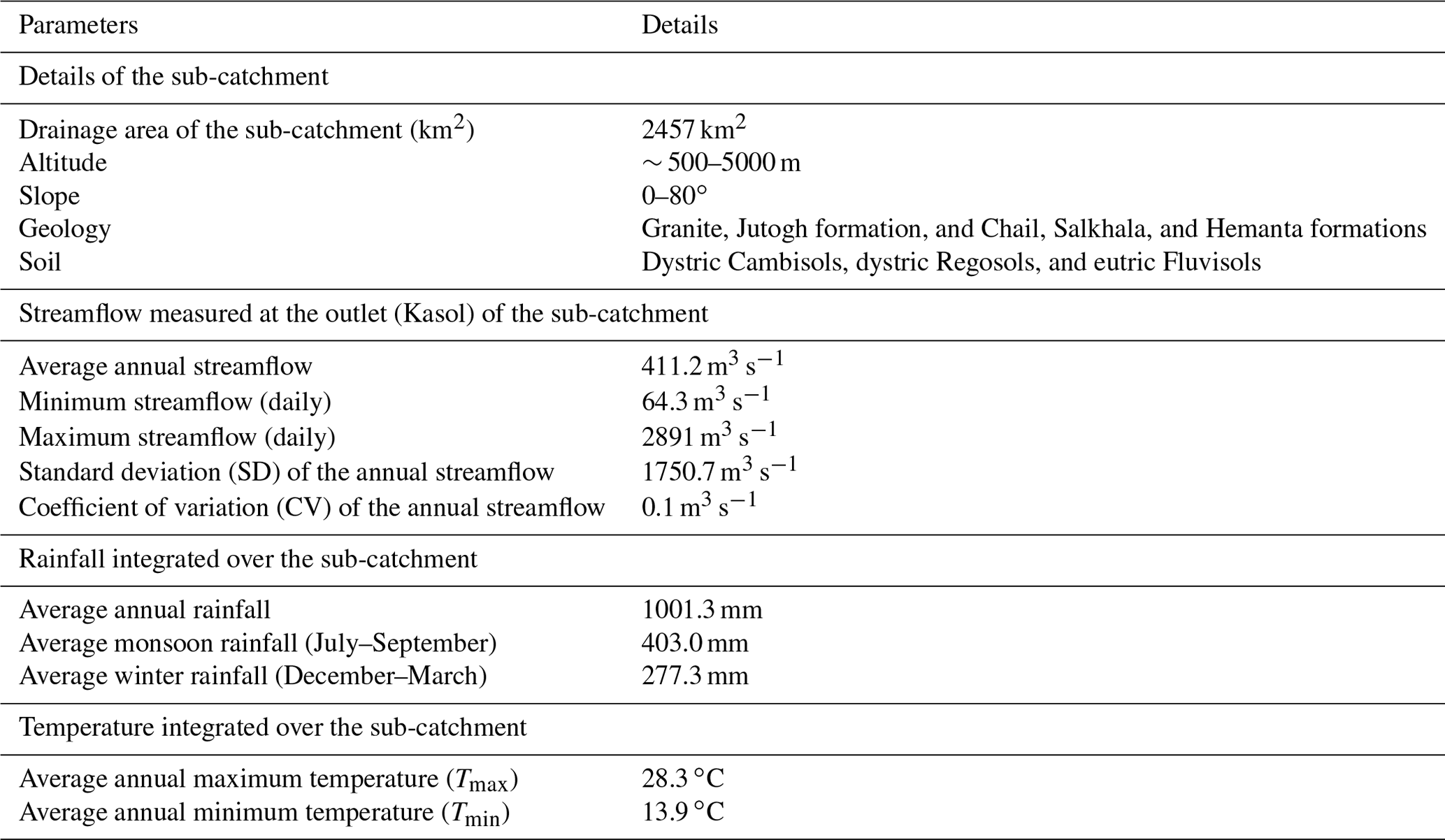
The selected study area is a sub-catchment within the Satluj basin (Fig. 1), with an area of 2457 km2. Topographically, it is very rugged (0–80∘) and is dominated mostly by forests (56.20 %), grassland (26.4 %), agricultural lands (17.1 %), and glaciers and snow cover (0.3 %; Singh et al., 2015a). The presence of mountain barriers in the sub-basin's north, the large variation in altitudes (500–5000 m), and the aspect all contribute to the region's diverse climate. It varies from a hot and moist tropical climate in the lower valleys to a cool temperate climate at about 2000 m and tends towards an alpine climate as the altitude increases beyond 2000 m. The mean annual discharge (averaged over the period of 1979–2009) of the river gauged at Kasol was 12 469.43 m3 s−1. There is a large inter-diurnal and monthly variation in the pattern of the river discharge. The minimum and maximum daily discharge recorded at Kasol was 64.30 and 2891 m3 s−1, respectively. The early months of the year, i.e. starting from January up to March, are characterised by low streamflow. After this, a continuous and rapid rise in flow occurs, with the maximum being in the month of July (∼ 22 %–23 %). Then, it again starts decreasing, and the flow reaches its minimum in the month of December (2 %–3 %). The details of the sub-catchment are summarised in Table 1.
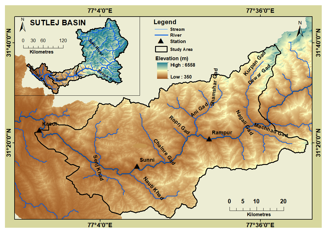
Figure 1The location of the sub-catchment within Sutlej River basin. The three hydrometeorological stations (Kasol, Sunni, and Rampur), from which this study employed observed data for the years 1979 to 2009, are also shown.
Table 1Characteristics of the study catchment over the evaluation period of 1979–2009.
The sub-basin is bestowed with large hydropower potential. There are three major hydroelectric power projects, namely the Sunni Dam Hydro Electric Project of 1080 MW,Rampur hydroelectric power plant (RHEP) of 412 MW, and Nathpa Jhakri India Hydroelectric Power Plant (NJHEP) of 1500 MW. The sub-basin is climatologically sensitive and, at present, facing challenges due to climate change and human interventions (Singh et al., 2015b, c). Changes in future climate will alter the patterns of flow in the river and could further affect the water resources and hydroelectric power production (Singh et al., 2014).
The methodology involved in predicting streamflow for the period 2041–2100 in the Sutlej River is included in Sect. 3.1, which is a collection of hydrometeorological data, Sect. 3.2, which is a selection of machine and deep learning models, Sect. 3.3, which is a performance evaluation of the developed models, and Sect. 3.4, which is a bias correction in the streamflow projection. These are described in detail under following sub-headings.
3.1 Hydrometeorological data
The daily rainfall, temperature (Tmax and Tmin), relative humidity, solar radiation, wind speed, and discharge data used to study the performance of the different machine and deep learning models on streamflow modelling were collected for 31 years, i.e. 1979–2009. Rainfall, temperature, and discharge data were obtained from the Bhakra Beas Management Board (BBMB), while relative humidity, solar radiation, and wind data were extracted from the Climate Forecast System Reanalysis (CFSR) Global Weather Data (http://globalweather.tamu.edu/, last access: 4 October 2020). These data were collected for three hydrometeorological stations, namely Kasol, Sunni, and Rampur (Fig. 1).
The downscaled outputs from the CMIP6 GCMs, the latest generation of climate models, were used for streamflow prediction in the future (2050s and 2080s). This framework of CMIP6 GCMs was run to simulate future climate under four Shared Socioeconomic Pathway (SSP) scenarios, which are designed to explain potential future greenhouse gas (GHG) emissions under various global socioeconomic shifts that could occur by 2100 (Riahi et al., 2017; Karan et. al, 2022). Even when using downscaled outputs, however, the regional climate change projections inherit biases from the GCM boundary conditions (Jose and Dwarakish, 2022), which were corrected in the dataset detailed in Mishra et al. (2020) for South Asia. They used the empirical quantile mapping (EQM) method to remove bias in the downscaled data. This dataset provides bias-corrected downscaled climate change projections for 13 CMIP6 GCMs and four GHG emission scenarios (SSP126, SSP245, SSP370, and SSP585), and the latter are briefly summarised in Riahi et al. (2017). Climate projections from CMIP6 GCMs that have been generated under the SSP245 and SSP585 scenarios are used in this study. SSP245, a medium scenario, represents the average pathway of future GHG emissions, with a radiative forcing of 4.5 W m−2 by the year 2100, while SSP585 is the scenario with an upper limit in the range of scenarios with a radiative forcing of 8.5 W m−2 by the end of this century (O'Neill et al., 2016). The data are available at a daily timescale and horizontal spatial resolution of 0.25∘ × 0.25∘. Seven grids of the downscaled CMIP6 GCM data cover the study area. The temperature (Tmax and Tmin) data were adjusted for topographical bias by separating the study area into a number of homogenous elevation bands spaced by at an interval of 1000 m and applying a temperature lapse rate of 6.5 ∘C per 1000 m within each grid. A digital elevation model (DEM) of 30 m spatial resolution derived from CartoSat-1 stereo data (http://www.bhuvan.nrsc.gov.in, last access: 20 November 2020) was used for this purpose. The values of rainfall and temperature at each grid were then averaged over the catchment, using the Thiessen polygon method, in order to provide daily rainfall data integrated at the catchment scale for assessing changes in the future climate with respect to the observed period, i.e. 1979–2009.

Figure 2Taylor diagram showing comparative skills of 13CMIP6 GCMs in simulating climatic variables (rainfall, Tmax, and Tmin) over the Sutlej sub-basin during reference period (1979–2009). The degree of the correlation coefficient (r) between the observed and CMIP6 GCMs, centred root mean square error (CRMSE), and departure of the models' standard deviation (SD) from the observed data (dashed black arc line) are shown in panel (a) for rainfall, panel (b) for Tmax, and panel (c) for Tmin. The units of SD for rainfall and temperature are in centimetres and degrees Celsius, respectively.
Furthermore, the ranking of CMIP6 GCMs was done to find the most appropriate models that can generate the most plausible scenarios of future climate in the catchment and, ultimately, be employed in the streamflow projection. A Taylor diagram (Taylor, 2001), a robust graphical plot, is widely used to rank GCMs due to its effectiveness in determining the relative strengths of the competing models and in evaluating overall performance as a model evolves (Abbasian et al., 2019; Ghimire et al., 2021). It integrates three statistical metrics, including the degree of correlation (r), centred root mean square error (CRMSE), and ratio of spatial standard deviation (SD). Combining these metrics allows the determination of the degree of pattern correspondence and explains how exactly a model represents the observed climate (Taylor, 2001). Therefore, the performance of 13 CMIP6 GCMs in modelling climatic variables (rainfall, Tmax, and Tmin) in the Sutlej sub-basin was compared to the observed data (1979–2009) using a Taylor diagram (Fig. 2a–c). The models were then ranked as a result of this comparison. A high positive correlation (r = 0.84 to 0.96) and low CRMSE (< 3 ∘C) error were found in all 13 CMIP6 GCMs for temperature (Tmax and Tmin; Fig. 2b–c). Additionally, it was found that the models' standard deviations, which ranged from 5.60 to 6.03 ∘C for Tmax and 6.34 to 6.63 ∘C for Tmin, were close to the SD of the observed data (6.01 and 6.07 ∘C). These results imply that all CMIP6 GCMs may be able to predict the most likely future temperature over the catchment.
However, not all CMIP6 GCMs showed the high degree of similarity in predicting rainfall; in fact, 2 (CanESM5 and NorESM2-LR) of the 13 models revealed a negative correlation (Fig. 2a). In the pool of 13 CMIP6 GCMs, only six models showed relatively higher correlation (r ≥ 0.56), smaller CRMSE (< 12 cm) errors, and a high similarity to the standard deviation of the observed data (13.2 cm). They were the (1) Earth Consortium Earth 3 Veg model (EC-Earth3-Veg), (2) Russian Institute for Numerical Mathematics climate model version 4.8 (INM-CM4-8), (3) Russian Institute for Numerical Mathematics climate model version 5.0 (INM-CM5-0), (4) Max Planck Institute for Meteorology Earth System Model version 1.2 with higher resolution (MPI-ESM1-2-HR), (5) Max Planck Institute for Meteorology Earth System Model version 1.2 with lower resolution (MPI-ESM1-2-LR), and (6) Norwegian Earth System Model version 2 with medium resolution (NorESM2-MR). Furthermore, within these models, the highest and lowest correlations between observed and simulated rainfall were found for the INM-CM4-8 (r = 0.69) and NorESM2-MR (r = 0.56), respectively. These six CMIP6 GCMs were finally selected to examine future patterns in streamflow for the periods 2050s and 2080s in the Sutlej River basin, as they had also shown high performance in simulating temperatures (r = 0.90 to 0.96).
3.2 Selection of machine learning and deep learning models for streamflow modelling
In this study, five machine learning models and one deep learning model, namely GLM, GAM, MARSs, ANN, RF and 1D convolution neural network (1D-CNN), were selected, and their performances in predicting streamflow in Sutlej River were compared. These are regression-based models which capture the relationship between the predictors (dependent variables) and the predictand (independent variables) and provide the value of the output variables (Adnan et al., 2019; Kabir et al., 2020). The models were trained with daily observed data recorded during 1979–2009 at Kasol (the gauging site) and simulated historical projections of CMIP6 GCMs. The climatic projections of the grid corresponding to the Kasol station were taken into consideration as the input from the CMIP6 GCMs. However, prior to building the models, all of the data were normalised, using standard normalisation techniques, to standardise the features on a common scale. Furthermore, the entire dataset was split into training and testing datasets, since a cross-validation method was adopted in this study. The training dataset (80 %) was used for fitting the models, whereas a testing dataset was used for checking model accuracy (20 %). Under the cross-validation method, the process was repeated until every part of the allocated data was used in testing (Kabir et al., 2020). Six different program codes were written in the Python language for ANN, GAM, GLM, MARSs, RF, and 1D-CNN simulations. Out of these six selected models, GLM, GAM, and MARSs are linear models, whereas other three i.e. ANN, RF, and 1D-CNN, are non-linear in nature (Shortridge et al., 2016; Yang et al., 2019; Herath et al., 2021). Additionally, excluding GLM, all of the remaining models are based on a non-parametric regression approach, where the functional relationship between the predictor and predictand is not predetermined but can be adjusted to capture the unusual or unexpected features of the data (Shortridge et al., 2016). A detailed description of these models can be found elsewhere (Shortridge et al., 2016; Adnan et al., 2019; Yang et al., 2019; Kabir et al., 2020; Ghimire et al., 2021; Herath et al., 2021; Shu et al.,2021).
Since the 1D-CNN model is based on weight sharing, it needs fewer training parameters than other models (Kiranyaz et al., 2021). It has mainly three layers, i.e. a convolution layer, pooling layer, and fully connected layer. The primary job of the convolution layer is to non-linearly map input data into a set of feature maps or a series of feature vectors. When working as a visual cortical perceptron, the filter kernels are convoluted with the input data of their receptive fields. The convolution results with biases are then passed on to the activation function to create feature maps. The pooling layer, which comes after each convolution layer, primarily serves to reduce the dimension of the feature maps and maintain the invariance of characteristic scale. The fully connected layer uses a completely connected single layer perceptron to combine the feature maps that were acquired by the prior convolution and pooling layers in order to build a higher-level feature (Kiranyaz et al., 2021). In this study, one convolution layer with 64 filters, a kernel of size 2, and a rectified linear activation function (ReLU) was employed. This was followed by max pooling layer with pool size of 2 and the faltterm layer. After that, two fully connected layers are applied with ReLU and a linear activation function, respectively. However, for optimisation, the adaptive moment estimation (Adam) algorithm was applied (Ghimire et al., 2021; Shu et al., 2021). Six variables, namely rainfall, Tmax, Tmin, relative humidity, solar radiation, and wind speed were used as input for developing the models. Additionally, to understand the control of the catchment size and geo-hydromorphological characteristics of the basin in generating runoff, these models were simulated under the following four rainfall scenarios: rainfall on the same day (R0), rainfall lagged by 1 d (R1), rainfall lagged by 2 d (R2), and rainfall lagged by 3 d (R3). The remaining meteorological parameters were held constant during the processes.

3.3 Model performance evaluation
It has been found that overfitting in a model may lead to large errors in out-of-sample predictions (Hastie et al., 2009). Therefore, it has been evaded by establishing model parameters for GLM, GAM, MARSs, ANN, and RF through automated hyperparameter tuning methods. In total, 500 bootstrapped resamples of the training dataset were generated for each parameter value to be assessed. Table 2 presents the information on the specific parameters evaluated for each model.
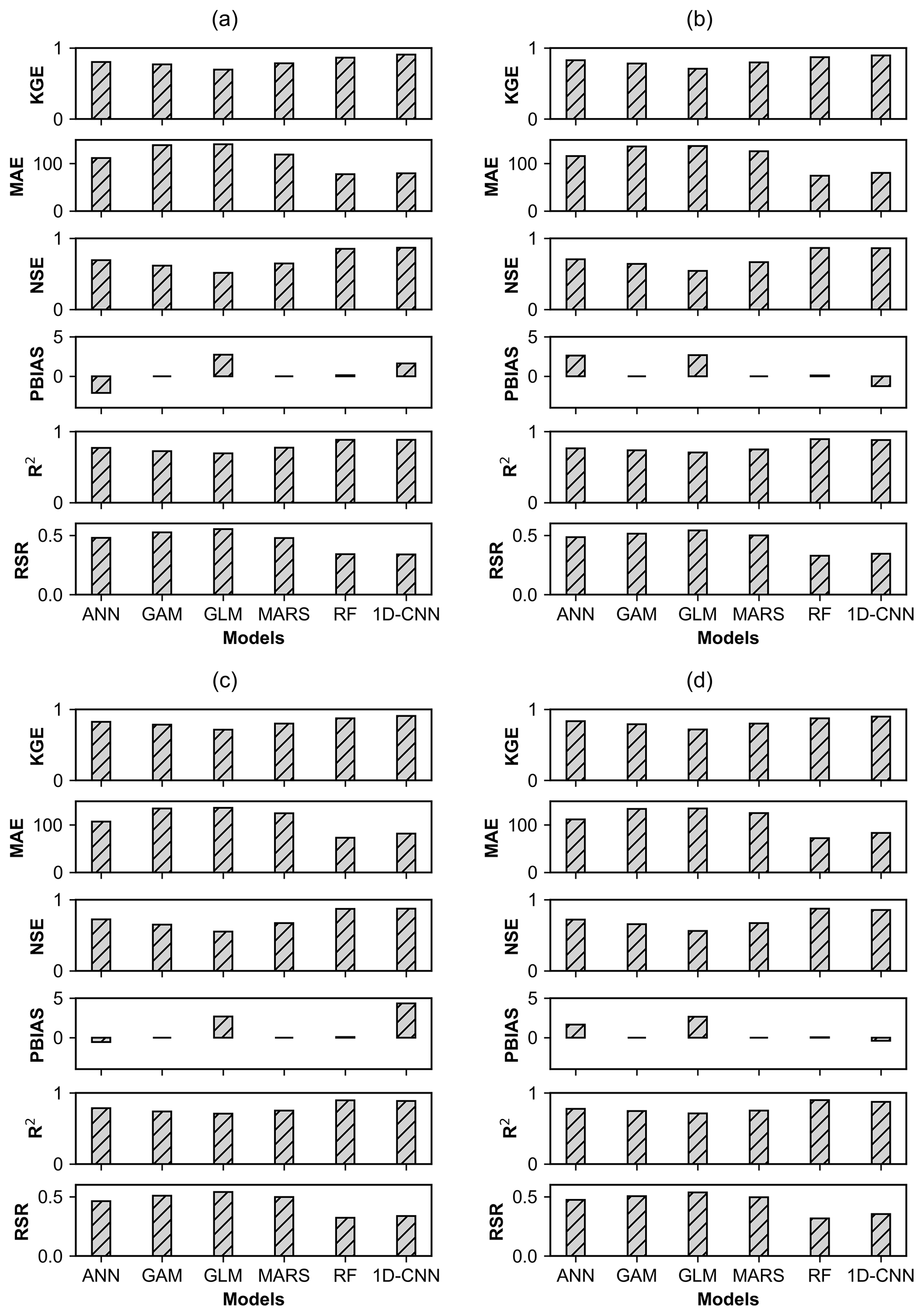
Figure 3Evaluation of the models' (ANN, GAM, GLM, MARSs, RF, and 1D-CNN) performance in simulating streamflow under rainfall scenarios (a) R0, (b) R1, (c) R2, and (d) R3 at Kasol during the training phase using six statistical metrics (R2, KGE, NSE, RSR, MAE, and PBIAS).
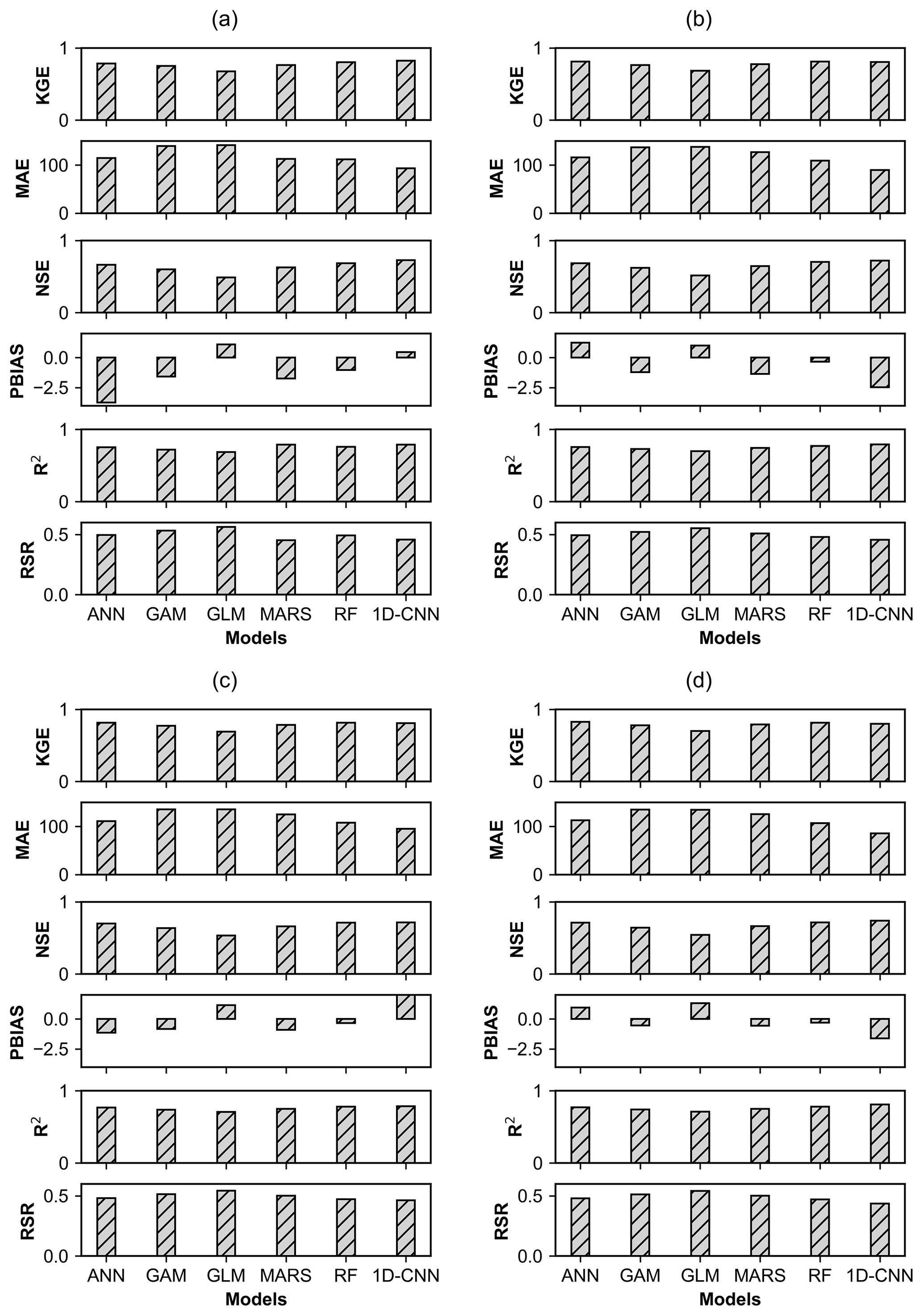
Figure 4Evaluation of the models' (ANN, GAM, GLM, MARSs, RF, and 1D-CNN) performance in simulating streamflow under rainfall scenarios (a) R0, (b) R1, (c) R2, and (d) R3 at Kasol during the testing phase using six statistical metrics (R2, KGE, NSE, RSR, MAE, and PBIAS).
The accuracy with which the simulated flow matches the observed flow during the training (calibration) and testing (validation) phases determines whether a hydrological model is appropriate for a given application (Refsgaard, 1997). Several methods, including quantitative statistics and graphical methods, have been developed in the past for assessing the accuracy of model predictions (Legates and McCabe, 1999). Moriasi et al. (2007) grouped these methods into three categories, namely standard regression, dimensionless, and error index, depending on how well each method explains the relationship between observed and simulated values, compares the relative performance of the models, and quantifies the deviation in the units of the data of interest. Moreover, it has been established from previous studies that a single metric is inadequate to evaluate a model's performance; hence, multiple metrics should be used (Adnan et al., 2020). Therefore, in this study, the prediction accuracy of different models was compared using six statistical measures, out of which one was a standard regression (coefficient of determination, R2), two of which were dimensionless (Kling–Gupta efficiency, KGE, and Nash–Sutcliffe efficiency, NSE), and the remaining three were the error index (ratio of the root mean square error to the standard deviation of the measured data, RSR, the mean absolute error, MAE, and the percent bias, PBIAS). These metrics are defined below by Eqs. (2)–(7):
where Pi are the predicted values, and Qi are the observed values. n accounts for the number of samples, represents the mean of the observed data, and is the mean of the predicted data. However, r is the Pearson's correlation coefficient, whereas σob and σp refer to the standard deviation of the observed and predicted values, respectively.
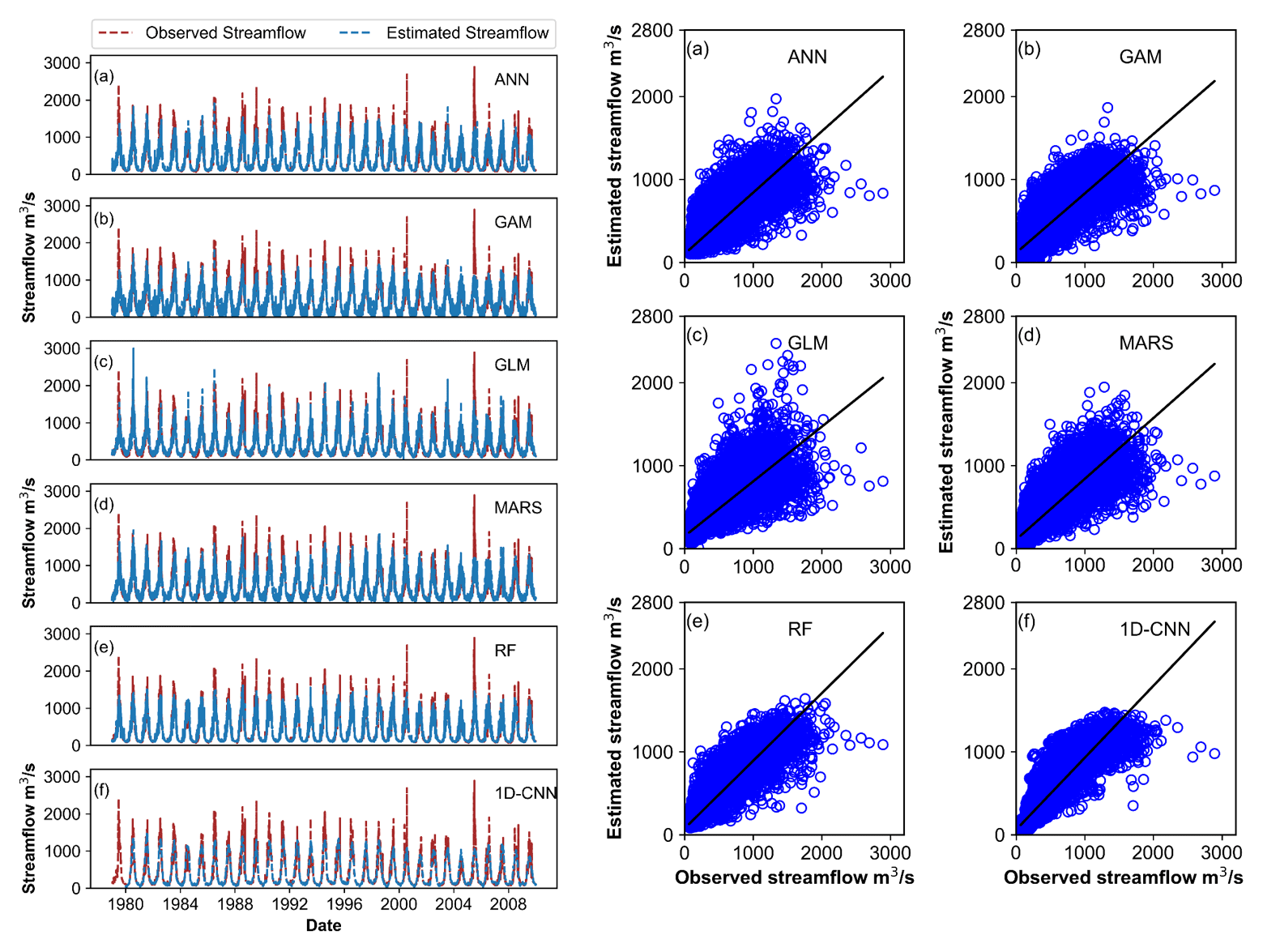
Figure 5Comparison of observed and simulated streamflow for all six models (ANN, GAM, GLM, MARSs, RF, and 1D-CNN) under rainfall scenarios R0.
R2 evaluates the percentage of the variation in the measured data that can be explained by the model, whereas the NSE estimates the relative size of the residual variance in relation to the variance in the measured data (Nash and Sutcliffe, 1970; Van-Liew et al., 2003). According to Mazrooei et al. (2021), the NSE is sensitive to extreme flows; as a result, the KGE is also used to evaluate a model's performance, while taking extreme flows into account (Adib and Harun, 2022). Other metrics, like RSR, MAE, and PBIAS, shed light on the overall inaccuracies in the projected flow relative to the observed. The values of R2, KGE, and NSE should all be 1 in an ideal model, whereas RSR, MAE, and PBIAS values should be 0 (Nash and Sutcliffe, 1970; Van-Liew et al., 2003; Gupta et al., 1999; Adnan et al., 2020). Moriasi et al. (2007) developed a guideline for interpreting the results of these metrics and a rank for the hydrological models based on a thorough review of the available literature. They found that a model can be classified as very good, good, satisfactory, or unsatisfactory if its NSE value is between 0.75 and 1, 0.65 and 0.75, 0.50 and 0.65, or less than 0.50, respectively. Similarly, R2 values between 0.6 and 0.7 are considered satisfactory, 0.85 and 1 are very good, and numbers below 0.5 are unsatisfactory (Van-Liew et al., 2003). However, for RSR, numbers above 0.7 are considered to be poor, whereas values between 0 and 0.5 are considered to be in the very good range. Thus, the lower the RSR value, the better the model. This is also true for PBIAS and MAE, where lower values are favourable. According to Moriasi et al. (2007), PBIAS values of less than ±10 % are considered to be highly acceptable, while values of more than ±25 % are considered to be unsatisfactory. The negative number indicates that the model has overestimated its bias, whereas the positive value indicates that the model has underestimated its bias (Gupta et al., 1999).
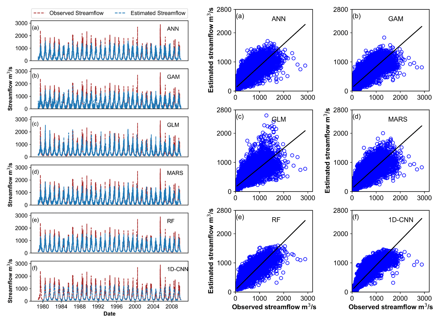
Figure 6A comparison of observed and simulated streamflow for all six models (ANN, GAM, GLM, MARSs, RF, and 1D-CNN) under rainfall scenarios R1.
3.4 Bias correction
Uncertainty in streamflow prediction may be caused by the GCM shortcomings (e.g. coarse spatial resolution, simplified physics and thermodynamic processes, numerical methods, or poor knowledge of climate system dynamics) in accurately replicating natural climate variability (Sperna Weiland et al., 2010). As a result, its quantification and correction are critical for generating a future time series of streamflow that is reliable and recommended for devising water resource management plans in the catchment. This study used the bias correction method proposed in Hawkins et al. (2013) to correct the uncertainty (bias) between observed and CMIP6-GCM-predicted streamflow. The mathematical expression for this formula is given below:
where Qbc and Qfuture are the bias-corrected and raw daily discharge for future simulation, respectively.
and are the mean discharge of observed and historical simulation for the reference period (1979–2009), respectively. σo and σp are the standard deviation in the observed and historical simulation for the reference period, respectively. This method captures the variability in both the observation and GCM simulations (Hawkins et al., 2013), which is the interest of this study.

Figure 7Comparison of observed and simulated streamflow for all six models (ANN, GAM, GLM, MARSs, RF, and 1D-CNN) under rainfall scenarios R2.
4.1 Streamflow simulation and evaluation of model performance
The simulation (1979–2009) results generated under different rainfall scenarios (R0, R1, R2, and R3) on a daily timescale for all six models (GLM, GAM, MARSs, ANN, RF, and 1D-CNN) during training and testing are shown in Figs. 3 and 4, respectively. The model performed slightly better during training than during testing periods. R2, NSE, and KGE values across models ranged from 0.69 to 0.90, 0.52 to 0.87, and 0.69 to 0.91 and from 0.69 to 0.81, 0.49 to 0.74, and 0.68 to 0.82 during training and testing, respectively. Likewise, it was found that RSR, MAE, and PBIAS varied from 0.31 to 0.55, from 71.95 to 123.25 m3 s−1, and from −2.11 % to +4.31 % during training, as well as from 0.56 to 0.46, from 123.06 to 106.64 m3 s−1, and from −3.74 % to +2.21 % during testing, respectively. Non-linear models (ANN, 1D-CNN, and RF) outperformed linear models (GAM and GLM) in runoff prediction under all rainfall scenarios (R0, R1, R2, and R3), with the exception of MARSs, which produced results that were more or less comparable with those of the ANN model. Figures 3–4 show that both models (RF and 1D-CNN) satisfy the performance requirements outlined by Moriasi et al. (2007), but RF slightly outperformed CNN in terms of the error index. R2, NSE, KGE, RSR, MAE, and PBIAS values for the RF model during the training ranged from 0.88 to 0.90, 0.85 to 0.87, 0.86 to 0.87, 0.32 to 0.34, 71.95 to 77.49 m3 s−1, and +0.03 % to +0.13 %, respectively. For the 1D-CNN, however, it varied from 0.87 to 0.89, 0.85 to 0.87, 0.90 to 0.91, 0.34 to 0.35, 80.29 to 83.14 m3 s−1, and −1.25 % to +0.13 %. A similar pattern with slightly lower values was revealed during testing for the both models. This implies that RF can effectively capture non-linear interactions and can provide insights about actual watershed functions (Shortridge et al., 2016). On the other hand, GLM showed the poorest results. R2, NSE, KGE, RSR, MAE, and PBIAS values for the GLM during the training varied from 0.69 to 0.71, 0.52 to 0.56, 0.71 to 0.72, 0.54 to 0.55, 134.80 to 140.56 m3 s−1, and +2.63 % to +2.73 %, respectively. During testing, they varied between 0.69 and 0.71, 0.49 and 0.54, 0.68 and 0.70, 0.54 and 0.56, 134.35 and 141.26 m3 s−1, and +1 % and +1.31 %, respectively. Furthermore, it was observed that the models with rainfall scenario R3 revealed reasonably better results in comparison to the R0, R1, and R2 scenarios, indicating the delayed contribution of rainfall–runoff to the river.
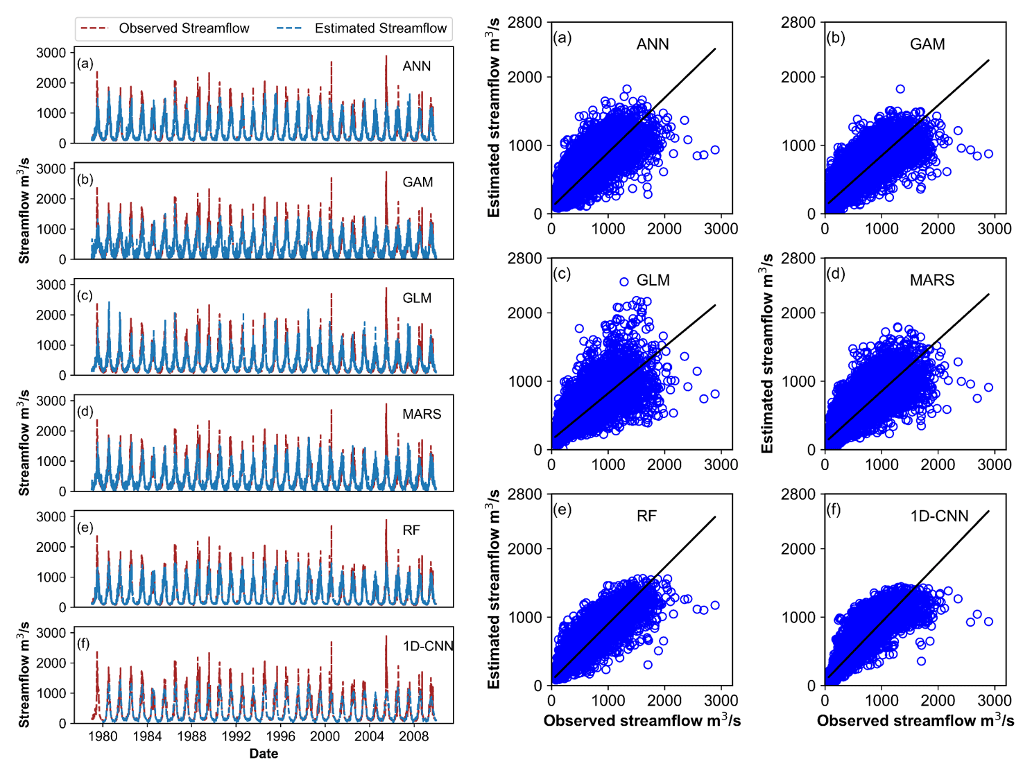
Figure 8Comparison of observed and simulated streamflow for all six models (ANN, GAM, GLM, MARSs, RF, and 1D-CNN) under rainfall scenarios R3.
Figures 5, 6, 7, and 8 show a comparison of the observed and simulated streamflow under rainfall scenarios of R0, R1, R2, and R3 for all the models at Kasol, which is the outlet of the basin. As observed in Figs. 5–8, RF was able to follow the curve better compared to the other models. It is also deduced from the comparison of scatterplots wherein a relatively smaller deviation in the observed and estimated discharge of streamflow was found for the RF model. GLM performed the worst out of the six models with respect to the time variation graphs. A limitation faced by all the six models was the simulation of peak values. The models slightly underperformed at the prediction of higher values of streamflow. These findings led to the ultimate decision to use the RF model with rainfall scenario R3 to predict streamflow in the Sutlej River in the future (2050s and 2080s) under the SSP245 and SSP585 scenarios.
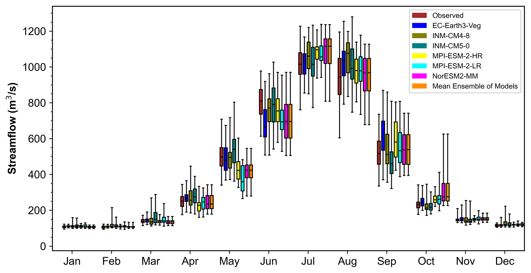
Figure 9Box plot comparing observed and CMIP6-GCM-simulated (mean ensemble of models) streamflow for various months of the year, as derived over the period 1979–2009. The line inside the box denotes the median values of the streamflow, while the upper and lower whiskers indicate the highest and minimum values, respectively.
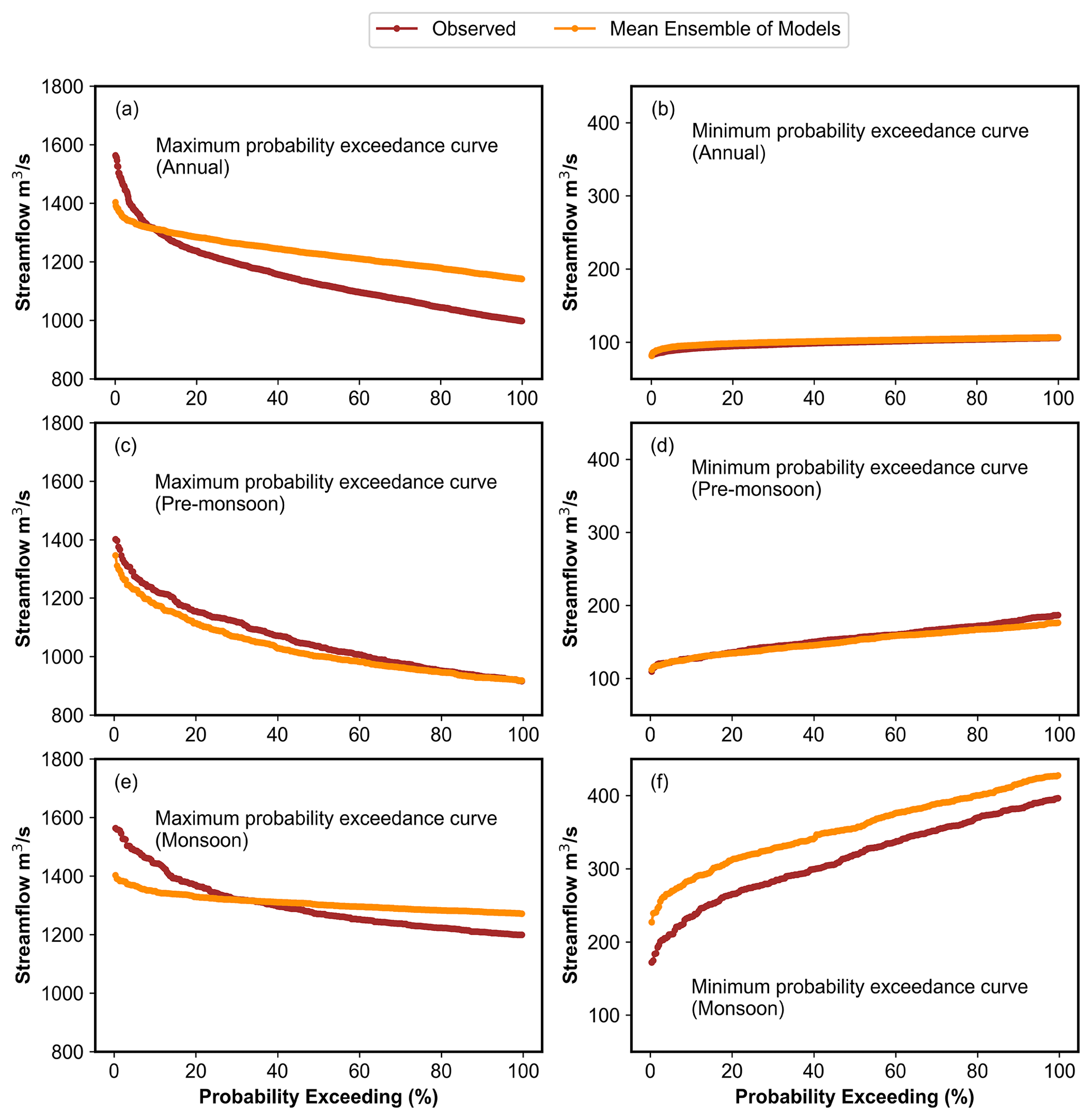
Figure 10Probability exceedance curves developed using 10 % of the highest and lowest flows from the observed and CMIP6-GCM-simulated (mean ensemble of models) flows over the time span of 1979–2009 for annual and seasonal (pre-monsoon and monsoon) flows.

Figure 11Projected change in the mean monthly rainfall in the sub-basin using different CMIP6 GCMs under the SSP245 and SSP585 scenarios in the (a, c) 2050s and (b, d) 2080s.
4.2 Comparison of streamflow simulated with observed and CMIP6 GCMs data
The uncertainty between observed and CMIP6-GCM-predicted streamflow during the reference period (1979–2009) was investigated by comparing the streamflow simulated by the RF model with the observed and CMIP6 GCM data. A large difference in streamflow patterns was seen in the box plot of observed and CMIP6-GCM-simulated discharge (Fig. 9) derived for various months of the year, particularly from June through September (monsoon season), when a pattern of intense daily rainfall was observed over the catchment. Additionally, it was discovered through the analysis of the probability exceedance curves generated using 10 % of the time series' highest flows that, despite the streamflow in the two datasets being comparable throughout the pre-monsoon season (Fig. 10c), they differ noticeably for high flows during the annual (Fig. 10a) and monsoon season (Fig. 10c). Similar trends were seen in the comparison of the probability exceedance curves for low flows during the monsoon season, although there was strong agreement for annual (Fig. 10b) and pre-monsoon measurements (Fig. 10d). This may be due to the fact that orography has a considerable impact on the regional Indian summer monsoon (ISM) climate, making it challenging for climate models to predict daily monsoonal rainfall accurately across the Himalaya (Turner and Annamalai, 2012; Niu et al., 2015; Choudhary et al., 2022). The regional climate model (RCM) based on CMIP5 GCMs was used by Sanjay et al. (2017) to study the pattern of change in precipitation and temperature over the Hindukush Himalaya region. As a condition of the model's inability to accurately represent complicated feedback mechanisms, the results revealed large uncertainty in the summer and winter precipitation over the northwestern Himalaya. This is also supported by the study of Kadel et al. (2018). They evaluated the performance of 38 CMIP5 GCMs in simulating rainfall over the central Himalaya and came to the conclusion that the majority of the models studied performed poorly when it came to reproducing the spatial distribution of monsoonal rainfall. Although the most recent study by Gusain et al. (2020) in India reported that an ISM simulation using CMIP6 GCMs over CMIP5 GCMs had significantly improved, there are discrepancies between the models, and this indicated uncertainty in the predictions. Lalande et al. (2021) examined the abilities of 26 CMIP6 GCMs to simulate the rate of precipitation across the Himalayan region and concluded that the models consistently overestimated the rate of precipitation by 31 % to 281 %. Additionally, a cold bias in temperature estimation was also reported. Therefore, bias correction, as described in Sect. 3.4, was applied to the projected streamflow for the future periods (2050s and 2080s) under all scenarios and for all six models in order to provide accurate times series of the discharge.
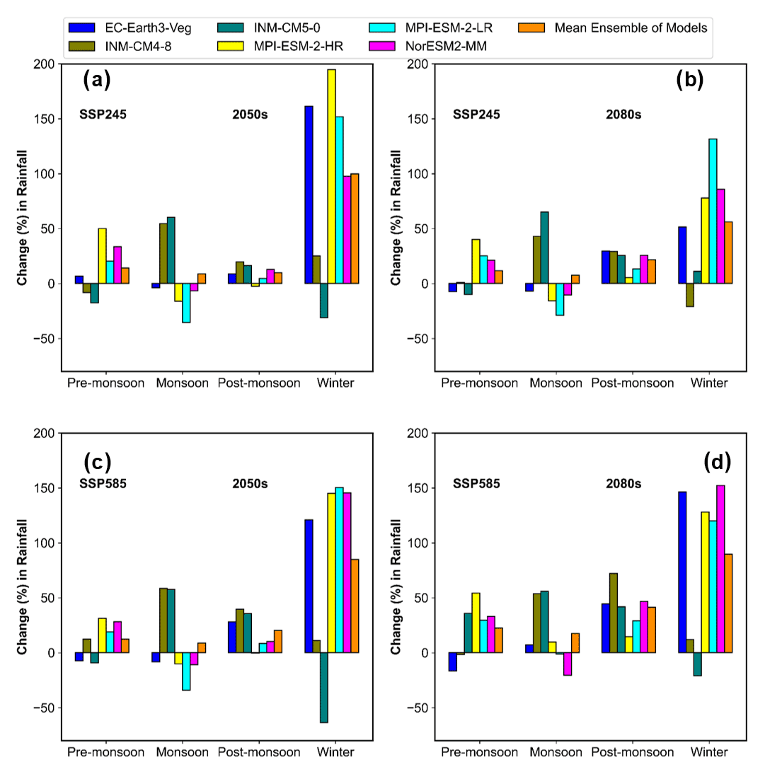
Figure 12Projected change in the mean seasonal rainfall in the sub-basin using different CMIP6 GCMs under the SSP245 and SSP585 scenarios in the (a, c) 2050s and (b, d) 2080s.
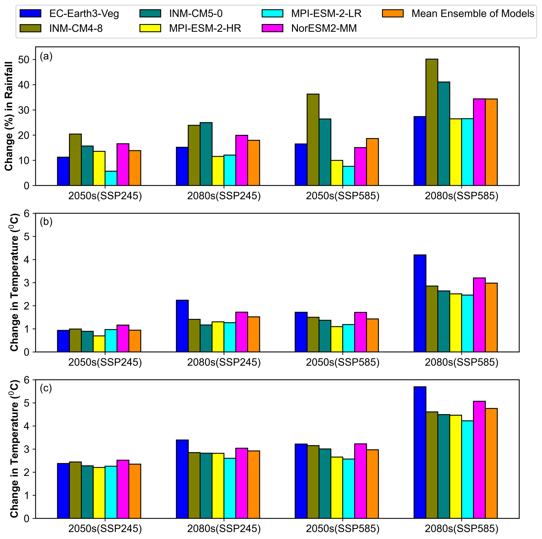
Figure 13Projected changes in the (a) mean annual rainfall, (b) Tmax, and (c) Tmin in the sub-basin using different CMIP6 GCMs under the SSP245 and SSP585 scenarios in the 2050s and 2080s.
4.3 Projected change in rainfall and temperatures in 2050s and 2080s under SSP245 and SSP585
Figure 11 shows how the catchment's mean monthly rainfall is expected to change under SSP245 and SSP585 in the 2050s and 2080s compared to the reference period (1979–2009). Within the months and for the CMIP6 GCMs, a sizeable shift in the rainfall pattern is seen. With the exception of March, June, and September, the mean ensemble of the models generally predicts a rise in rainfall throughout the year in the 2050s and 2080s under all scenarios. The models also show a significant variation in the seasonal and yearly rainfall patterns expected for the catchment in the 2050s and 2080s under various emission scenarios. However, based on the mean ensemble of the models, it is predicted that seasonal (Fig. 12) and annual (Fig. 13a) rainfall will generally increase in the 2050s and 2080s under SSP245 and SSP585. Pre-monsoon, monsoon, post-monsoon, and winter rainfall in the 2050s will increase by 8.75 % to 8.85 %, 10 % to 20.80 %, 85 % to 91.91 %, and 12.48 % to 14.16 %, respectively, under SSP245 and SSP585. However, under SSP245 and SSP585 in the 2080s, it will rise by 7.69 % to 17.50 %, 21.52 % to 41.43 %, 56.16 % to 89.66 %, and 22.48 % to 12.43 %, respectively. Under both scenarios in the 2050s and 2080s, the pre-monsoon and post-monsoon will have the lowest and highest percentage increases in rainfall, respectively. The monsoon season is, however, anticipated to have the greatest rise in terms of quantity (∼ 40–167 mm). The predicted range for the increase in mean annual rainfall is 13.85 % to 18.61 % in the 2050s and 17.91 % to 34.31 % in the 2080s. It is observed that the predicted pattern of change in rainfall across the sub-basin under various SSPs is consistent in terms of the direction of change with other studies conducted over the Sutlej and Himalaya region. Lalande et al. (2021) reported an overall increase in the mean annual precipitation over the Himalayan region based on 10 CMIP6 GCMs. According to their analysis, the mean ensemble of model precipitation is predicted to increase by 8.6 % to 25.4 % in 2081–2100 under SSP245 and SSP585. The same study also showed an increase in the region's winter (November to April) and ISM (June to September) rainfall. This contradicts past studies that showed a trend towards declining ISM rainfall after the 1950s (Sabin et al., 2020). They postulated that the region's higher winter rainfall would have been caused by the strengthening of the western disturbances; however, the intensification of the ISM is responsible for the region's enhanced summer rainfall.
The analysis of the CMIP6 GCM projections leads to the conclusion that, for all months and seasons in the 2050s and 2080s, maximum (excluding April and pre-monsoon in the 2050s under SSP245) and minimum temperatures will rise under both scenarios (Figs. 14a–d and 15a–d). Similarly, increase in mean annual Tmin and Tmax is also predicted in the 2050s and 2080s under all scenarios (Fig. 13b and c). The increase will be relatively higher for the Tmin compared to the Tmax. This is also reported by Singh et al. (2015c). The increase in rainfall and temperature is typically higher under SSP585 than SSP245 in both eras (2050s and 2080s), as expected, due to a larger increase in radiative forcing brought on by increased greenhouse gas emissions.
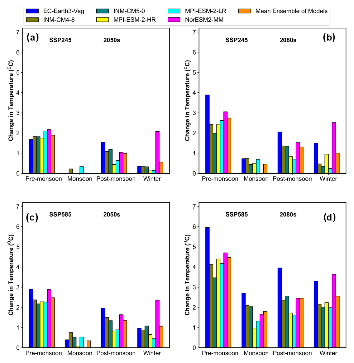
Figure 14Projected change in the mean seasonal maximum temperature (Tmax) in the sub-basin using different CMIP6 GCMs under the SSP245 and SSP585 scenarios in the (a, c) 2050s and (b, d) 2080s.

Figure 15Projected changes in the mean seasonal minimum temperature (Tmin) in the sub-basin using different CMIP6 GCMs under the SSP245 and SSP585 scenarios in the (a, c) 2050s and (b, d) 2080s.
4.4 Assessment of the change in streamflow in 2050s and 2080s under SSP245 and SSP585
The Sutlej River's mean monthly streamflow change, compared to the reference period's observed flow (1979–2009), is shown in Fig. 16 under scenarios SSP245 and SSP585 for the future periods (2050s and 2080s). According to both scenarios and all six models, the Sutlej River's streamflow will decrease between January (−33.80 % to −14.38 %), February (−32.40 % to −14.15 %), March (−23.55 % to −0.84 %), November (−21.06 % to −5.14 %), and December (−29.88 % to −18.38 %) in the 2050s and 2080s. Moreover, except for MPI-ESM1-2-HR and MPI-ESM1-2-LR, which show an increase in streamflow in the 2080s under the higher-emission scenario, all of the CMIP6 GCMs indicate a decrease in the river's discharge in June (−20.24 % to −0.57 %) under SSP245 and SSP585 for both the periods. Similarly, excluding EC-Earth3-Veg (under SSP245 in 2050s) and INM-CM5-0 (under SSP245 in the 2050s and 2080s and under SSP585 in the 2050s), all of the CMIP6 GCMs indicate a decrease in the river's discharge in May (−25 % to −2.85 %) during the study period. In contrast, under SSP245 and SSP585 in the 2050s and 2080s, all of the CMIP6 GCMs predict a rise in the river's discharge in April (20.24 % to −0.57 %; excluding SSP585 in the 2080s), August (16.84 % to 5.28 %), and September (55.27 % to 4.35 %). But no clear pattern of streamflow change is seen for the remaining months (July and October) of the year, making results difficult to generalise because the projected decrease and/or increase in streamflow over the months is inconsistent among models under various emission scenarios in the 2050s and 2080s. The variations in climate-variable projections caused by differing spatial resolutions and parameterisation levels in the climate models may be the cause of these discrepancies in streamflow estimates (Sperna Weiland et al., 2010; Singh et al., 2015a). According to Murphy et al. (2004), the average of an ensemble of GCMs cancels out the errors in each individual model, and as more models are used, the ensemble uncertainty decreases. Therefore, in order to reduce the uncertainty in the projection of streamflow related to individual CMIP6 GCMs, the streamflow pattern of the Sutlej River was analysed by also using the mean ensemble of all six GCMs.
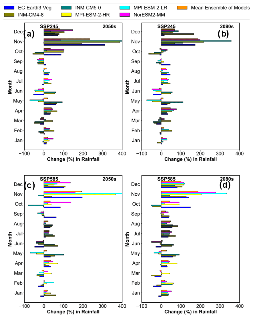
Figure 16Predicted change in monthly streamflow pattern of the Sutlej River with respect to the reference period (1979–2009) in (a, b) 2050s and (c, d) 2080s under SSP245 and SSP585 scenarios for different CMIP6 GCMs.
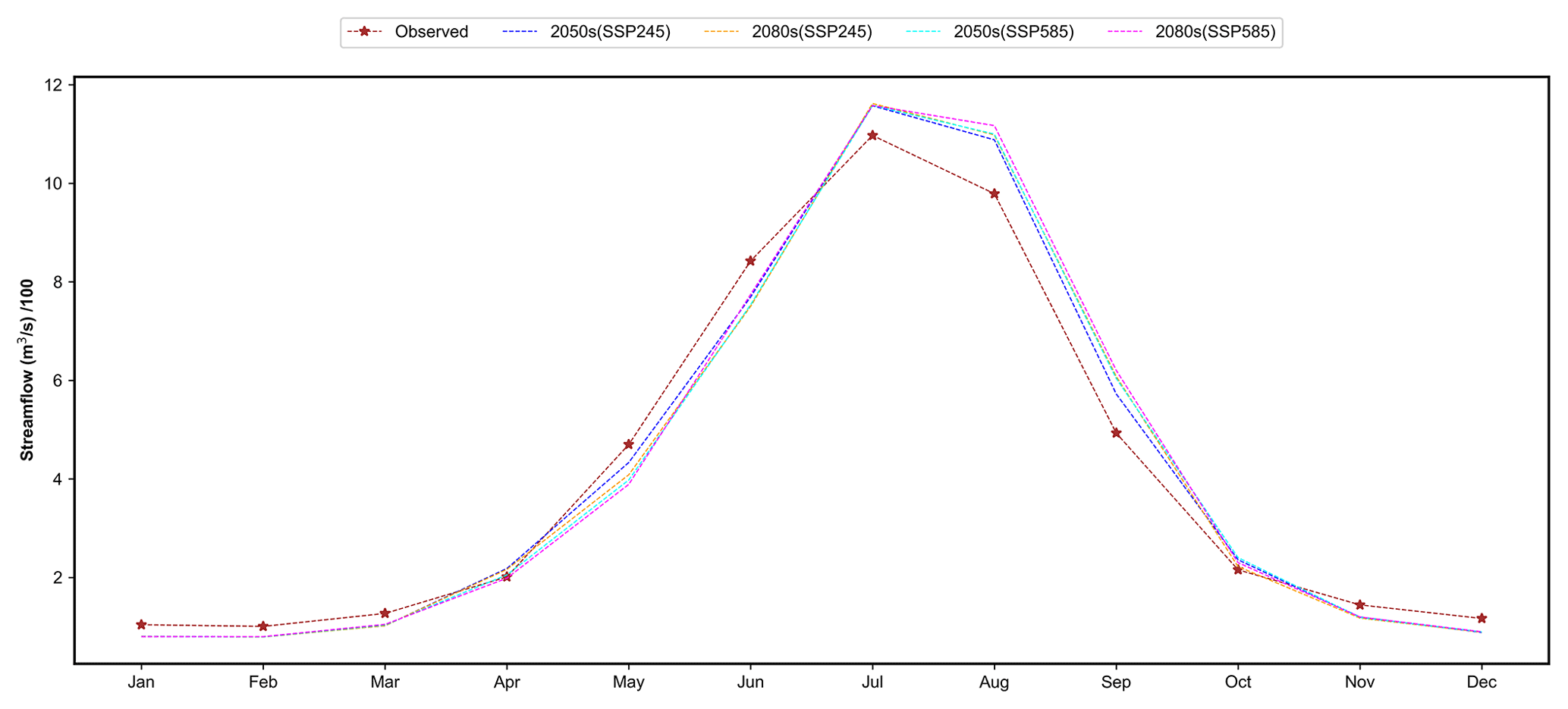
Figure 17Comparison of monthly observed (1979–2009) and projected discharge of the multimodel ensembles for the 2050s and 2080s under the SSP245 and SSP585 scenarios.
The mean ensemble of the models predicts that the Sutlej River's mean monthly streamflow (excluding April) will decrease under both scenarios from November (−18.45 % to −17.17 %) to June (−10.90 % to −8.06 %) between the 2050s and 2080s (Fig. 17). The river flow, which would have been expected to increase in April under both scenarios in 2050s, will also decline in the 2080s for the higher emission scenarios (SPP585). The maximum and minimum streamflow declines are predicted to occur in the 2050s under SSP245 for the months of December (−24.25 %) and May (−7.77 %), respectively. In comparison to SPP245, the decline will generally be slightly higher under SSP585 in 2050s, and for the 2080s, the projected decrease in streamflow will not show much difference under both the scenarios. Opposite to this, the mean ensemble of the models predicts that the Sutlej River's flow will increase from July (5.50 % to 5.91 %) to October (3.01 % to 11.42 %) in the 2050s and 2080s under both scenarios. The maximum and minimum streamflow increases are predicted to occur in the 2080s under SSP245 for the months of September (25.82 %) and July (5.50 %), respectively. In all scenarios, the increase will be slightly greater in the 2080s than it will be in the 2050s. When compared to SPP245, it will be higher for SSP585 in the scenarios.
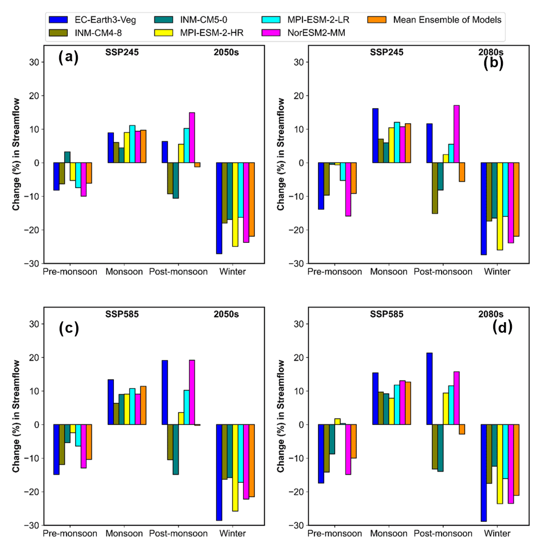
Figure 18Predicted change in seasonal streamflow pattern of the Sutlej River with respect to the reference period (1979–2009) in the (a, c) 2050s and (b, d) 2080s under the SSP245 and SSP585 scenarios for different GCMs.
The projected change in the seasonal streamflow of the Sutlej River in 2050s and 2080s is shown in Fig. 18. The 2050s and 2080s would see an increase in streamflow during the monsoon (4.46 % to 16.14 %) and a decrease during the pre-monsoon (−17.40 % to −0.51 %) and winter (−28.81 % to −12.42 %) for all six CMIP6 GCMs, with the exception of INM-CM5-0 in the 2050s under SSP245 and MPI-ESM1-2-HR and MPI-ESM1-2-LR in the 2080s under SPP585, which indicate an increase rather than a decrease in streamflow during the pre-monsoon. The predicted streamflow for the post-monsoon season, however, does not show a consistent pattern of change across time within the models under SSP245 and SSP585 scenarios. But there is a high probability, based on the mean ensembles of models projections, that streamflow will also decline during the post-monsoon in 2050s (−1.23 % to −0.22 %) and 2080s (−5.59 % to −2.83 %) under all scenarios. Similarly, the predicted decline for pre-monsoon and winter will be between −10.36 % and −6.12 % and −21.87 % and −21.52 % under SSP245 and between −10.0 % and −9.13 % and −21.87 % and −21.11 % under SSP585, respectively. With the exception of winter, when there are no significant differences in the projected streamflow, the decline will be slightly larger in the 2080s than in the 2050s in all scenarios. In addition, the results of the mean ensemble of the models indicate that the Sutlej River's flow will increase during the monsoon under both scenarios, from 9.70 % to 11.41 % in the 2050s and 11.64 % to 12.70 % in the 2080s.
Similarly, Fig. 19 lists the projected change in the mean annual streamflow for the Sutlej River in 2050s and 2080s with respect to the reference period (1979–2009) under different emission scenarios. Although the nature of the direction of change within models varies, the mean ensemble of the models reveals a persistent increasing pattern in the streamflow for all scenarios in 2050s and 2080s. The Sutlej River's annual streamflow will rise between 2050 and 2080 by 0.79 % to 1.43 % for SSP585 and 0.87 % to 1.10 % for SSP245, according to the mean ensemble of the models. The rise is expected to be higher in the 2080s as compared to 2050s under SSP585.
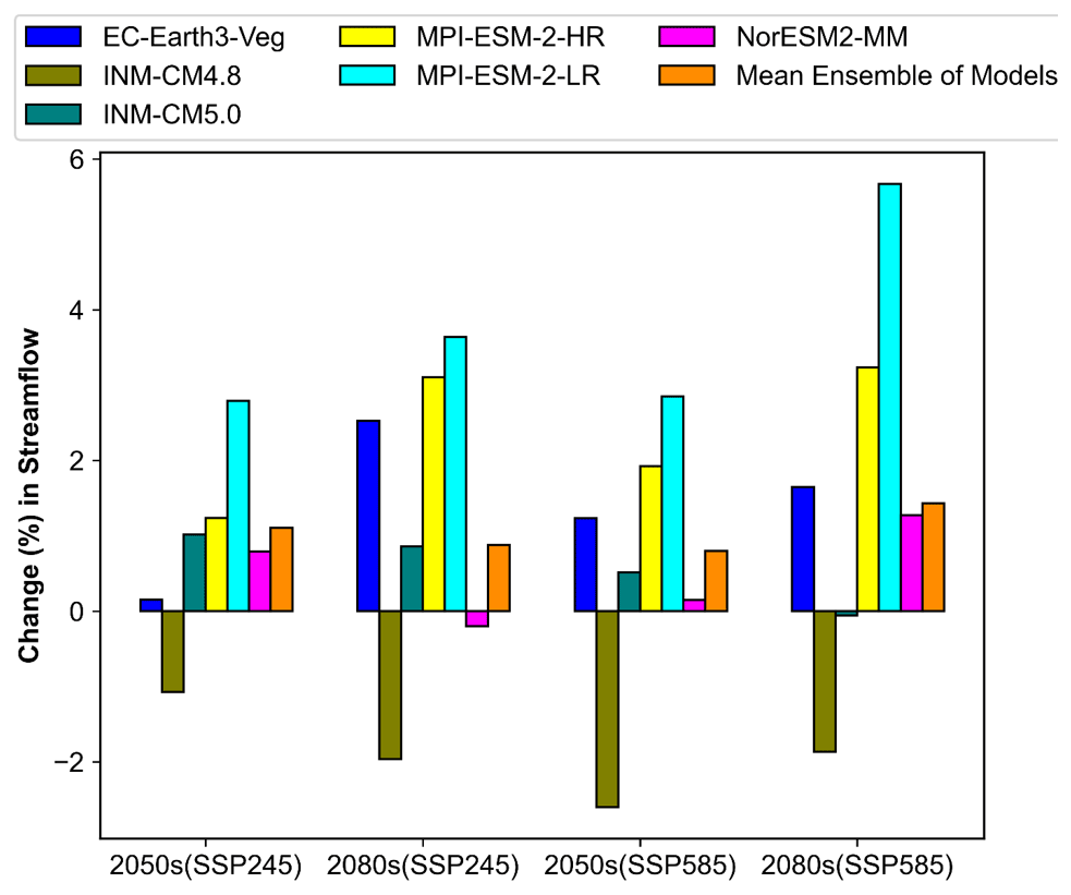
Figure 19Predicted change in the mean annual streamflow of the Sutlej River with respect to the reference period (1979–2009) in the 2050s and 2080s under SSP245 and SSP585 scenarios for different GCMs.
This study reveals an increase in the Sutlej River's mean annual and monsoonal streamflow in the 2050s and 2080s, which is in contrast to earlier studies (Singh et al., 2014; Ali et al., 2018) that reported a reduction based on long-term investigation of station data over historical era. The pattern of rainfall and temperature predicted by CMIP6 GCMs for the future periods under the SSP245 and SSP585 emission scenarios, in addition to the physical processes occurring within the basin, have contributed to this increase in the Sutlej River's streamflow. For instance, it is speculated that the projected increase in the mean streamflow during the monsoon season under both scenarios in the 2050s and 2080 for all models is related to the projected percentage increase in the rainfall amount over the catchment and the melting of glaciers brought on by the increased maximum and minimum temperatures. On the one hand, this increase in river streamflow and its propensity to raise the silt load may have an impact on both the capacity of reservoirs and the hydropower potential of hydroelectric facilities situated in the sub-basin and downstream of it. On the other hand, despite the predicted increase in rainfall throughout the pre-monsoon, post-monsoon, and winter seasons, the anticipated decrease in streamflow of the Sutlej River during pre-monsoon, post-monsoon, and winter may be explained by the projected rise in temperatures, which may have led to increased evaporation from the surface. Similar conclusions were reached by Adib and Harun (2022), who studied the Kurau River in Malaysia and predicted a drop in streamflow during the months of January, April, and October, despite receiving more rainfall. Moreover, during winter and post-monsoon, most of the precipitation in upper part of the catchment occurs in the form of snowfall, which has a minimal effect on the runoff generation in the catchment. Additionally, the large increase in monsoonal streamflow predicted during study periods is what led to the projected increase in the Sutlej River's mean annual flow. Predicted decreases in the Sutlej River streamflow over the pre-monsoon (April to June) and winter (December to March) seasons may have a significant impact on agriculture and hydropower generation downstream of the river, which is already struggling due to water shortages at this time of year. Ali et al. (2018) predicted that the hydroelectric production from the Nathpa Jhakri and Bhakra Nangal hydropower projects will decline during May to June in the future due to a projected decline in the streamflow of the Sutlej River.
The projected streamflow patterns for the Sutlej River under SSP245 and SSP585 scenarios in the 2050s and 2080s show similar tendencies, but with differing magnitudes, that have been found by past researchers using process-based hydrological models. For instance, Singh et al. (2015a) used the SWAT (Soil Water Assessment Tool) model, a semi-distributed hydrological model, to simulate streamflow for future periods using two CMIP3 GCMs (CGCM3 and HadCM3), and they discovered that the Sutlej River's mean annual streamflow would increase in the range of 0.6 % to 7.8 % for the future periods (2050s and 2080s). Similar to this, using the variable infiltration capacity (VIC) and SWAT models, respectively, Ali et al. (2018) and Shukla et al. (2021) estimated increases in the Sutlej River's mean annual streamflow for the 2050s and 2080s under RCP4.5 and RCP8.5. The study of Shukla et al. (2021) estimated that, under RCP4.5 and RCP8.5, the mean streamflow of the river would increase by 14 % and 21 % (at Rampur), respectively, in the 2080s. The previous studies observed that a substantially higher increase in projected streamflow may be attributable to the overestimation by the CMIP3 GCMs and CMIP5 GCMs of monsoonal precipitation over the Himalayan region (Choudhary et al., 2022; Sanjay et al., 2017; Gusain et al., 2020; Lalande et al., 2021). Similar to this, the results of Singh et al. (2015a), Ali et al. (2018), and Shukla et al. (2021) corroborated the expected decrease in streamflow during pre-monsoon and winter in addition to a rise during monsoon. This suggests that the RF model can accurately predict runoff and analyse the effects of climate change, while capturing the non-linearity of a hilly catchment.
This study compared the performance of the five machine learning models (GLM, GAM, MARSs, ANN, and RF) and one deep learning model (1D-CNN), which were further divided into linear (MARSs, ANN, and RF) and non-linear (ANN, 1D-CNN, and RF) models, in simulating rainfall–runoff responses over the hilly Sutlej River basin in order to determine the best model for predicting streamflow response to future climate change in the 2050s and 2080s under SSP245 and SSP585 using CMIP6 GCM data. The important findings of the study are summarised below.
-
In general, non-linear models (ANN, 1D-CNN, and RF) outperformed linear models (GAM, GLM, and MARSs) in runoff prediction under all rainfall scenarios (R0, R1, R2, and R3). Among all the models, RF and 1D-CNN were identified as being the best models as per the model evaluation criteria. However, RF outperformed CNN in terms of error index (MAE and PBIAS), and as a result, it was used to investigate impact of future climate change on the Sutlej River pattern in the 2050s and 2080s under the SSP245 and SSP585 emission scenarios.
-
The developed RF model slightly underperformed at the prediction of higher values of streamflow during training and testing. This implies that it is less effective at predicting flash floods that are caused by intense rainfall in the catchment. However, it was determined that the results produced by RF were comparable to process-based hydrological models for a long-term change study in streamflow pattern.
-
Significant variations in the streamflow pattern were observed throughout the periods of months, seasons, and years and for the CMIP6 GCMs. The differences in the spatial resolution and parameterisation levels of CMIP6 GCMs, which caused a noticeable change in the projected amounts of temperature and precipitation during the study periods, may serve as an illustration of these variances in streamflow prediction. The Sutlej River's mean annual streamflow, based on the mean ensemble of models, is predicted to rise between the years 2050 and 2080 by 0.79 % to 1.43 % for SSP585 and by 0.87 % to 1.10 % for SSP245. Additionally, under both emission scenarios, streamflow will decrease during the pre- and post-monsoon (−1.23 % to −0.22 % and −5.59 % to −2.83 %) and during the winter (−21.87 % to −21.52 % and −21.87 % to −21.11 %) but increase during the monsoon (9.70 % to 11.41 % and 11.64 % to 12.70 %) in the 2050s and 2080s.
-
The increase in the Sutlej River's streamflow (annual and monsoon) is due to both physical processes that occur within the basin and rainfall and temperature patterns that are predicted by CMIP6 GCMs for future time periods under the SSP245 and SSP585 emission scenarios. On the one hand, the projected rise in mean streamflow during the monsoon season is associated with both the projected percentage increase in rainfall over the catchment and the melting of glaciers brought on by the increasing maximum and minimum temperatures. On the other hand, the predicted increase in temperatures, which may have led to increased evaporation from the surface, may be used to explain the anticipated reduction in streamflow of the Sutlej River during pre-monsoon, post-monsoon, and winter.
-
Additionally, the projected changes in the mean annual and seasonal streamflow of the river are consistent with earlier research done using process-based physical hydrological models. Thus, the outcomes of the overall study indicate that the RF model is efficient for simulating streamflow in the Himalayan catchment and that water availability during monsoon will rise as a result of an increase in catchment precipitation, which would eventually lead to an increased sediment load and affect hydropower generation. However, the predicted reduction in streamflow during pre-monsoon, post-monsoon, and winter will put stress on agriculture and hydropower generation downstream of the river, which is already struggling due to water shortages at this time of year. The administrators of local water resources and the government organisations in charge of maintaining reservoirs downriver may find these details on streamflow patterns to be of great use.
The codes developed for this study can be made available to the readers on reasonable request to the corresponding author.
The observed station data are confidential, and the authors do not have permission to share the data.
DS and SL conceptualised the problems, supervised the entire research activity from its inception to its completion, contributed to the data collection, processing, and interpretation, and wrote the research paper. MV and RS contributed to the development of the model, generation of figures, and analysis of data. PC and DC contributed to the data analysis and interpretation.
The contact author has declared that none of the authors has any competing interests.
Publisher’s note: Copernicus Publications remains neutral with regard to jurisdictional claims in published maps and institutional affiliations.
This article is part of the special issue “Hydrological response to climatic and cryospheric changes in high-mountain regions”. It is not associated with a conference.
The authors acknowledge the National Natural Science Foundation of China (NFSC; grant no. 42171129), for funding this research work, and the Bhakra Beas Management Board (BBMB), India, for the hydrometeorological data used in this study. We thank Pratibha Shrivastava, a fourth-year computer science student (B. Tech) at NIT Raipur, for her help in building the model.
This research has been supported by the National Natural Science Foundation of China (grant no. 42171129).
This paper was edited by Yue-Ping Xu and reviewed by two anonymous referees.
Abbasian, M., Moghim, S., and Abrishamchi, A.: Performance of the general circulation models in simulating temperature and precipitation over Iran, Theor. Appl. Climatol., 135, 1465–1483, https://doi.org/10.1007/s00704-018-2456-y, 2019.
Adib, M. N. M. and Harun, S.: Metalearning Approach Coupled with CMIP6 Multi-GCM for Future Monthly Streamflow Forecasting, J. Hydrol. Eng., 27, 05022004, https://doi.org/10.1061/(ASCE)HE.1943-5584.0002176, 2022.
Adnan, R. M., Yuan, X., Kisi, O., Yuan, Y., Tayyab, M., and Lei, X.: Application of soft computing models in streamflow forecasting. In Proceedings of the institution of civil engineers-water, Manage., 172, 123–134, https://doi.org/10.1680/jwama.16.00075, 2019.
Adnan, R. M., Liang, Z., Heddam, S., Zounemat-Kermani, M., Kisi, O., and Li, B.: Least square support vector machine and multivariate adaptive regression splines for streamflow prediction in mountainous basin using hydro-meteorological data as inputs, J. Hydrol., 586, 124371, https://doi.org/10.1016/j.jhydrol.2019.124371, 2020.
Ali, S. A., Aadhar, S., Shah, H. L., and Mishra, V.: Projected increase in hydropower production in India under climate change, Sci. Rep., 8, 1–12, https://doi.org/10.1038/s41598-018-30489-4, 2018.
Archer, D.: Contrasting hydrological regimes in the upper Indus Basin, J. Hydrol., 274, 198–210, https://doi.org/10.1016/S0022-1694(02)00414-6, 2003.
Beven, K. J.: Rainfall-runoff modelling: the primer, John Wiley & Sons, ISBN 978-0-470-71459-1, 2011.
Chen, H., Sun, J., Lin, W., and Xu, H.: Comparison of CMIP6 and CMIP5 models in simulating climate extremes, Sci. Bull., 65, 1415–1418, https://doi.org/10.1016/j.scib.2020.05.015, 2020.
Choudhury, B. A., Rajesh, P. V., Zahan, Y., and Goswami, B. N.: Evolution of the Indian summer monsoon rainfall simulations from CMIP3 to CMIP6 models, Clim. Dynam., 58, 2637–2662, https://doi.org/10.1007/s00382-021-06023-0, 2022.
Conan, C., De Marsily, G., Bouraoui, F., and Bidoglio, G.: A long-term hydrological modelling of the Upper Guadiana River basin (Spain), Phys. Chem. Earth. A/B/C, 28, 193–200, https://doi.org/10.1016/S1474-7065(03)00025-1 2003.
Dai, A., Qian, T., Trenberth, K. E., and Milliman, J. D.: Changes in continental freshwater discharge from 1948 to 2004, J. Climate, 22, 2773–2792, https://doi.org/10.1175/2008JCLI2592.1, 2009.
Das, J. and Nanduri, U. V.: Assessment and evaluation of potential climate change impact on monsoon flows using machine learning technique over Wainganga River basin, India, Hydrol. Sci. J., 63, 1020–1046, https://doi.org/10.1080/02626667.2018.1469757, 2018.
Easterling, D. R., Meehl G, A., Parmesan, C., Changnon S, A., Karl, T. R., and Mearns, L. O.: Climate extremes: observations, modeling, and impacts, Science, 289, 2068–2074, https://doi.org/10.1126/science.289.5487.2068, 2000.
Eng, K. and Wolock D. M.: Evaluation of machine learning approaches for predicting streamflow metrics across the conterminous United States, No. 2022-5058, US Geological Survey, https://doi.org/10.3133/sir20225058, 2022.
Fu, M., Fan, T., Ding Z, A., Salih S, Q., Al-Ansari, N., and Yaseen Z. M.: Deep learning data-intelligence model based on adjusted forecasting window scale: application in daily streamflow simulation, IEEE Access., 8, 32632–32651, https://doi.org/10.1109/ACCESS.2020.2974406, 2020.
Gao, Y., Gao, X., and Zhang, X.: The 2 ∘C global temperature target and the evolution of the long-term goal of addressing climate change – from the United Nations framework convention on climate change to the Paris agreement, Engineering, 3, 272–278, https://doi.org/10.1016/J.ENG.2017.01.022, 2017.
Gerten, D., Rost, S., von Bloh, W., and Lucht, W.: Causes of change in 20th century global river discharge, Geophys. Res. Lett., 35, L20405, https://doi.org/10.1029/2008GL035258, 2008.
Ghimire, S., Yaseen, Z. M., Farooque, A. A., Deo, R. C., Zhang, J., and Tao, X.: Streamflow prediction using an integrated methodology based on convolutional neural network and long short-term memory networks, Sci. Rep., 11, 1–26, https://doi.org/10.1038/s41598-021-96751-4, 2021.
Ghobadi, F. and Kang, D.: Improving long-term streamflow prediction in a poorly gauged basin using geo-spatiotemporal mesoscale data and attention-based deep learning: A comparative study, J. Hydrol., 615, 128608, https://doi.org/10.1016/j.jhydrol.2022.128608, 2022.
Goswami, B. N., Venugopal, V., Sengupta, D., Madhusoodanan, M. S., and Xavier, P. K.: Increasing trend of extreme rain events over India in a warming environment, Science., 314, 1442–1445, https://doi.org/10.1126/science.1132027, 2006.
Gupta, H. V., Sorooshian, S., and Yapo, P. O.: Status of automatic calibration for hydrologic models: Comparison with multilevel expert calibration, J. Hydrol. Eng., 4, 135–143, 1999.
Gusain, A., Ghosh, S., and Karmakar, S.: Added value of CMIP6 over CMIP5 models in simulating Indian summer monsoon rainfall, Atmos. Res., 232, 104680, https://doi.org/10.1016/j.atmosres.2019.104680, 2020.
Haddeland, I., Heinke, J., Biemans, H., Eisner, S., Flörke, M., Hanasaki, N., Konzmann, M., Ludwig, F., Masaki, Y., Schewe, J., and Stacke, T.: Global water resources affected by human interventions and climate change, P. Natl. Acad. Sci. USA, 111, 3251–3256, https://doi.org/10.1073/pnas.1222475110, 2014.
Hagen, J. S., Leblois, E., Lawrence, D., Solomatine, D., and Sorteberg, A.: Identifying major drivers of daily streamflow from large-scale atmospheric circulation with machine learning, J. Hydrol., 596, 126086, https://doi.org/10.1016/j.jhydrol.2021.126086, 2021.
Hastie, T., Tibshirani, R., Friedman, J. H., and Friedman, J. H.: The elements of statistical learning: data mining, inference, and prediction, Vol. 2, 1–758, Springer, New York, https://www.sas.upenn.edu/~fdiebold/NoHesitations/BookAdvanced.pdf (last access: 24 July 2022), 2009.
Hawkins, E., Osborne, T. M., Ho, C. K., and Challinor, A. J.: Calibration and bias correction of climate projections for crop modelling: an idealised case study over Europe, Agr. Forest Meteorol., 170, 19–31, https://doi.org/10.1016/j.agrformet.2012.04.007, 2013.
Herath, H. M. V. V., Chadalawada, J., and Babovic, V.: Hydrologically informed machine learning for rainfall–runoff modelling: towards distributed modelling, Hydrol. Earth Syst. Sci., 25, 4373–4401, https://doi.org/10.5194/hess-25-4373-2021, 2021.
Hussain, D. and Khan, A. A.: Machine learning techniques for monthly river flow forecasting of Hunza River, Pakistan, Earth. Sci. Inf., 13, 939–949, https://doi.org/10.1007/s12145-020-00450-z, 2020.
Hussain, D., Hussain, T., Khan, A. A., Naqvi, S. A. A., and Jamil, A.: A deep learning approach for hydrological time-series prediction: A case study of Gilgit river basin, Earth. Sci. Inf., 13, 915–927, 2020.
Jose, D. M. and Dwarakish, G. S.: Bias Correction and trend analysis of temperature data by a high-resolution CMIP6 Model over a Tropical River Basin, Asia-Pac. J. Atmos. Sci., 58, 97–115, https://doi.org/10.1007/s13143-021-00240-7, 2022.
Kabir, S., Patidar, S., and Pender, G.: Investigating capabilities of machine learning techniques in forecasting stream flow, in: Proceedings of the Institution of Civil Engineers-Water Manage., 173, 69–86, https://doi.org/10.1680/jwama.19.00001, 2020.
Kadel, I., Yamazaki, T., Iwasaki, T., and Abdillah M, R.: Projection of future monsoon precipitation over the central Himalayas by CMIP5 models under warming scenarios, Clim. Res., 75, 1–21, https://doi.org/10.3354/cr01497, 2018.
Karan, K., Singh, D., Singh, P. K., Bharati, B., Singh, T. P., and Berndtsson, R.: Implications of future climate change on crop and irrigation water requirements in a semi-arid river basin using CMIP6 GCMs, J. Arid. Land., 14, 1234–1257, https://doi.org/10.1007/s40333-022-0081-1, 2022.
Kim, Y. H., Min, S. K., and Zhang, X.: Evaluation of the CMIP6 multi-model ensemble for climate extreme indices, Weat. Clim. Extremes, 29, 100269, https://doi.org/10.1016/j.wace.2020.100269, 2020.
Kiranyaz, S., Avci, O., Abdeljaber, O., Ince, T., Gabbouj, M., and Inman, D. J.: 1D convolutional neural networks and applications: A survey, Mech. Syst. Signal Pr., 151, 107398, https://doi.org/10.1016/j.ymssp.2020.107398, 2021.
Kirchner, J. W.: Getting the right answers for the right reasons: Linking measurements, analyses, and models to advance the science of hydrology, Water. Resour. Res., 42, W03S04, https://doi.org/10.1029/2005WR004362, 2006.
Krysanova, V.,Wortmann, M., Bolch, T., Merz, B., Duethmann, D., Walter, J., Huang, S., Tong, J., Buda, S., and Kundzewicz, Z. W.: Analysis of current trends in climate parameters, river discharge and glaciers in the Aksu River basin (Central Asia), Hydrol. Sci. J., 60, 566–590, https://doi.org/10.1080/02626667.2014.925559, 2015.
Kundzewicz, Z. W., Nohara, D., Tong, J., Oki, T., Buda, S., and Takeuchi, K.: Discharge of large Asian rivers–Observations and projections, Quat. Int., 208, 4–10, https://doi.org/10.1016/j.quaint.2009.01.011, 2009.
Lalande, M., Ménégoz, M., Krinner, G., Naegeli, K., and Wunderle, S.: Climate change in the High Mountain Asia in CMIP6, Earth Syst. Dynam., 12, 1061–1098, https://doi.org/10.5194/esd-12-1061-2021, 2021.
Legates, D. R. and McCabe Jr., G. J.: Evaluating the use of “goodness-of-fit” measures in hydrologic and hydroclimatic model validation, Water. Resour. Res., 35, 1, 233–241, https://doi.org/10.1029/1998WR900018, 1999.
Lutz, A. F., Immerzeel, W. W., Shrestha, A. B., and Bierkens, M. F. P.: Consistent increase in High Asia's runoff due to increasing glacier melt and precipitation, Nat. Clim. Change., 4, 587–592, https://doi.org/10.1038/nclimate2237, 2014.
Lutz, A. F., Ter Maat, H. W., Wijngaard, R. R., Biemans, H., Syed, A., Shrestha, A. B., Wester, P., and Immerzeel, W. W.: South Asian River basins in a 1.5 C warmer world, Reg. Enviro. Change., 19, 833–847, https://doi.org/10.1007/s10113-018-1433-4, 2019.
Mahato, P. K., Singh, D., Bharati, B., Gagnon, A. S., Singh, B. B., and Brema, J.: Assessing the impacts of human interventions and climate change on fluvial flooding using CMIP6 data and GIS-based hydrologic and hydraulic models, Geocarto. Int., 37, 11483–11508, https://doi.org/10.1080/10106049.2022.2060311, 2022.
Mazrooei, A., Sankarasubramanian, A., and Wood, A. W.: Potential in improving monthly streamflow forecasting through variational assimilation of observed streamflow, J. Hydrol., 600, 126559, https://doi.org/10.1016/j.jhydrol.2021.126559, 2021.
Miller, J. D., Immerzeel, W. W., and Rees, G.: Climate change impacts on glacier hydrology and river discharge in the Hindu Kush–Himalayas, Mt. Res. Dev., 32, 461–467, https://doi.org/10.1659/MRD-JOURNAL-D-12-00027.1, 2012.
Mishra, V., Bhatia, U., and Tiwari, A. D.: Bias-corrected climate projections for South Asia from Coupled Model Intercomparison Project-6, Sci. Data, 7, 338, https://doi.org/10.1038/s41597-020-00681-1, 2020.
Moriasi, D. N., Arnold, J. G., Van-Liew, M. W., Bingner, R. L., Harmel, R. D., and Veith, T. L.: Model evaluation guidelines for systematic quantification of accuracy in watershed simulations, T. ASABE, 50, 885–900, https://doi.org/10.13031/2013.23153, 2007.
Murphy, J. M., Sexton, D. M., Barnett, D. N., Jones, G. S., Webb, M. J., Collins, M., and Stainforth, D. A.: Quantification of modelling uncertainties in a large ensemble of climate change simulations, Nature, 430, 768–772, https://doi.org/10.1038/nature02771, 2004.
Nash, J. E. and Sutcliffe, J. V.: River flow forecasting through conceptual models part I – A discussion of principles, J. Hydrol., 10, 282–290, https://doi.org/10.1016/0022-1694(70)90098-3, 1970.
Nepal, S. and Shrestha, A. B.: Impact of climate change on the hydrological regime of the Indus, Ganges and Brahmaputra River basins: a review of the literature, Int. J. Water. Resou. Dev., 31, 201–218, https://doi.org/10.1080/07900627.2015.1030494, 2015.
Niu, X., Wang, S., Tang, J., Lee, D. K., Gutowski, W., Dairaku, K., McGregor, J., Katzfey, J., Gao, X., Wu, J., and Hong, S.: Projection of Indian summer monsoon climate in 2041–2060 by multiregional and global climate models, J. Geophys. Res.-Atmos., 120, 1776–1793, https://doi.org/10.1002/2014JD022620, 2015.
Oki, T. and Kanae, S.: Global hydrological cycles and world water resources, Science, 313, 1068–1072, https://doi.org/10.1126/science.1128845, 2006.
O'Neill, B. C., Tebaldi, C., van Vuuren, D. P., Eyring, V., Friedlingstein, P., Hurtt, G., Knutti, R., Kriegler, E., Lamarque, J.-F., Lowe, J., Meehl, G. A., Moss, R., Riahi, K., and Sanderson, B. M.: The Scenario Model Intercomparison Project (ScenarioMIP) for CMIP6, Geosci. Model Dev., 9, 3461–3482, https://doi.org/10.5194/gmd-9-3461-2016, 2016.
Otto, F. E., Skeie, R. B., Fuglestvedt, J. S., Berntsen, T., and Allen, M. R.: Assigning historic responsibility for extreme weather events, Nat. Clim. Change., 7, 757–759, https://doi.org/10.1038/nclimate3419, 2017.
Pasquini, A. I. and Depetris, P. J.: Discharge trends and flow dynamics of South American rivers draining the southern Atlantic seaboard: An overview, J. Hydrol., 333, 385–399, https://doi.org/10.1016/j.jhydrol.2006.09.005, 2007.
Rahimzad, M., Moghaddam Nia, A., Zolfonoon, H., Soltani, J., Danandeh Mehr, A., and Kwon, H. H.: Performance comparison of an lstm-based deep learning model versus conventional machine learning algorithms for streamflow forecasting, Water. Resour. Manage., 35, 4167–4187, https://doi.org/10.1007/s11269-021-02937-w, 2021.
Rasouli, K., Hsieh, W. W., and Cannon, A. J.: Daily streamflow forecasting by machine learning methods with weather and climate inputs, J. Hydrol, 414, 284–293, https://doi.org/10.1016/j.jhydrol.2011.10.039, 2012.
Refsgaard, J. C.: Parameterisation, calibration and validation of distributed hydrological models, J. Hydrol., 198, 69–97, https://doi.org/10.1016/S0022-1694(96)03329-X, 1997.
Riahi, K., Van Vuuren, D. P., Kriegler, E., Edmonds, J., O'Neill, B. C., Fujimori, S., Bauer, N., Calvin, K., Dellink, R., Fricko, O., Lutz, W., Popp, A., Cuaresma, J. C., Sameer, K. C., Leimbach, M., Jiang, L., Kram, T., Rao, S., Emmerling, J., Ebi, K., Hasegawa, T., Havlik, P., Humpenöder, H., Da Silva, L. A., Smith, S., Stehfest, E., Bosetti, V., Eom, J., Gernaat, D., Masui, T., Rogelj, J., Strefler, J., Drouet, L., Krey, V., Luderer, G., Harmsen, M., Takahashi, K., Baumstark, L., Doelman, J. C., Kainuma, M., Klimont, Z., Marangoni, G., Lotze-campen, H., Obersteiner, M., Tabeau, A., and Tavoni, M.: The shared socioeconomic pathways and their energy, land use, and greenhouse gas emissions implications: an overview, Global Environ. Change, 42, 153–168, https://doi.org/10.1016/j.gloenvcha.2016.05.009, 2017.
Sabin, T. P., Krishnan, R., Vellore, R., Priya, P., Borgaonkar, H. P., Singh, B. B., and Sagar, A.: Climate change over the Himalayas. In Assessment of climate change over the Indian region, Springer, Singapore, 207–222, https://doi.org/10.1007/978-981-15-4327-2_11, 2020.
Sanjay, J., Krishnan, R., Shrestha, A. B., Rajbhandari, R., and Ren, G. Y.: Downscaled climate change projections for the Hindu Kush Himalayan region using CORDEX South Asia regional climate models, Adv. Clim. Change. Res., 8, 185–198, https://doi.org/10.1016/j.accre.2017.08.003, 2017.
Schreiner-McGraw, A. P. and Ajami, H.: Impact of uncertainty in precipitation forcing data sets on the hydrologic budget of an integrated hydrologic model in mountainous terrain, Water. Resour. Res., 56, e2020WR027639, https://doi.org/10.1029/2020WR027639, 2020.
Shortridge, J. E., Guikema, S. D., and Zaitchik, B. F.: Machine learning methods for empirical streamflow simulation: a comparison of model accuracy, interpretability, and uncertainty in seasonal watersheds, Hydrol. Earth Syst. Sci., 20, 2611–2628, https://doi.org/10.5194/hess-20-2611-2016, 2016.
Shu, X., Ding, W., Peng, Y., Wang, Z., Wu, J., and Li, M.: Monthly streamflow forecasting using convolutional neural network. Water Resour. Manag., 35, 5089–5104, https://doi.org/10.1007/s11269-021-02961-w, 2021.
Shukla, S., Jain, S. K., and Kansal, M. L.: Hydrological modelling of a snow/glacier-fed western Himalayan basin to simulate the current and future streamflows under changing climate scenarios, Sci. Total. Environ., 795, 148871, https://doi.org/10.1016/j.scitotenv.2021.148871, 2021.
Singh, D., Gupta, R. D., and Jain, S. K.: Study of long-term trend in river discharge of Sutlej River (NW Himalayan region), Geogr. Environ. Sustain., 7, 87–96, https://doi.org/10.24057/2071-9388-2014-7-3-50-57, 2014.
Singh, D., Gupta, R. D., and Jain, S. K.: Assessment of impact of climate change on water resources in a hilly river basin, Arabian J. Geosci., 8, 10625–10646, https://doi.org/10.1007/s12517-015-1985-2, 2015a.
Singh, D., Gupta, R. D., and Jain, S. K.: Statistical analysis of long term spatial and temporal trends of temperature parameters over Sutlej River basin, India, J. Earth. Syst. Sci., 124, 17–35, https://doi.org/10.1007/s12517-015-1985-2, 2015b.
Singh, D., Jain, S. K., and Gupta, R. D.: Statistical downscaling and projection of future temperature and precipitation change in middle catchment of Sutlej River Basin, India, J. Earth. Syst. Sci., 124, 843–860, https://doi.org/10.1007/s12040-015-0575-8, 2015c.
Singh, D., Rai, S. P., and Rai, D.: Application of geospatial techniques in hydrological modelling, in: Sustainable Green Technologies for Environmental Management, edited by: Shah, S., Venkatramanan, V., and Prasad, R., Springer, Singapore, https://doi.org/10.1007/978-981-13-2772-8_8, 2019.
Singh, D., Zhu, Y., Liu, S., Srivastava, P. K., Dharpure, J. K., Chatterjee, D., Sahu, R., and Gagnon, A. S.: Exploring the links between variations in snow cover area and climatic variables in a Himalayan catchment using earth observations and CMIP6 climate change scenarios, J. Hydrol., 608, 127648, https://doi.org/10.1016/j.jhydrol.2022.127648, 2022.
Singh, P. and Jain, S. K.: Snow, and glacier melt in the Satluj River at Bhakra Dam in the western Himalayan region, Hydrol. Sci. J., 47, 93–106, https://doi.org/10.1080/02626660209492910, 2002.
Sood, A. and Smakhtin, V.: Global hydrological models: a review, Hydrol. Sci. J., 60, 549–565, https://doi.org/10.1080/02626667.2014.950580, 2015.
Sperna Weiland, F. C., van Beek, L. P. H., Kwadijk, J. C. J., and Bierkens, M. F. P.: The ability of a GCM-forced hydrological model to reproduce global discharge variability, Hydrol. Earth Syst. Sci., 14, 1595–1621, https://doi.org/10.5194/hess-14-1595-2010, 2010.
Stahl, K., Hisdal, H., Hannaford, J., Tallaksen, L. M., van Lanen, H. A. J., Sauquet, E., Demuth, S., Fendekova, M., and Jódar, J.: Streamflow trends in Europe: evidence from a dataset of near-natural catchments, Hydrol. Earth Syst. Sci., 14, 2367–2382, https://doi.org/10.5194/hess-14-2367-2010, 2010.
Stahl, K., Tallaksen, L. M., Hannaford, J., and van Lanen, H. A. J.: Filling the white space on maps of European runoff trends: estimates from a multi-model ensemble, Hydrol. Earth Syst. Sci., 16, 2035–2047, https://doi.org/10.5194/hess-16-2035-2012, 2012.
Taylor, K. E.: Summarizing multiple aspects of model performance in a single diagram, J. Geophys. Res.-Atmos., 106, 7183–7192, https://doi.org/10.1029/2000JD900719, 2001.
Thapa, S., Li, H., Li, B., Fu, D., Shi, X., Yabo, S., Lu, L., Qi, H., and Zhang, W.: Impact of climate change on snowmelt runoff in a Himalayan basin, Nepal, Environ. Monit. Assess., 193, 1–17, https://doi.org/10.1007/s10661-021-09197-6, 2021.
Trenberth, K. E.: Changes in precipitation with climate change, Clim. Res., 47, 123–138, https://doi.org/10.3354/cr00953, 2011.
Trenberth, K. E., Fasullo, J. T., and Shepherd, T. G. Attribution of climate extreme events, Nat. Clim. Change, 5, 725–730, https://doi.org/10.1038/nclimate2657, 2015.
Turner A, G. and Annamalai, H.: Climate change and the South Asian summer monsoon, Nat. Clim. Change, 2, 587–595, https://doi.org/10.1038/nclimate1495, 2012.
Van, S. P., Le, H. M., Thanh, D. V., Dang, T. D., Loc, H. H., and Anh, D. T.: Deep learning convolutional neural network in rainfall–runoff modelling, J. Hydroinf., 22, 541–561, https://doi.org/10.2166/hydro.2020.095, 2020.
Van der Wiel, K., Wanders, N., Selten, F. M., and Bierkens, M. F. P.: Added value of large ensemble simulations for assessing extreme river discharge in a 2 ∘C warmer world, Geophys. Res. Lett., 46, 2093–2102, https://doi.org/10.1029/2019GL081967, 2019.
Van-Liew, M. W., Arnold, J. G., and Garbrecht, J. D.: Hydrologic simulation on agricultural watersheds: Choosing between two models, T. ASAE, 46, 1539, https://doi.org/10.13031/2013.15643, 2003.
Wang, T., Zhao, Y., Xu, C., Ciais, P., Liu, D., Yang, H., Piao, S., and Yao, T.: Atmospheric dynamic constraints on Tibetan Plateau freshwater under Paris climate targets, Nat. Clim. Change, 11, 219–225, https://doi.org/10.1038/s41558-020-00974-8, 2021.
Xenarios, S., Gafurov, A., Schmidt-Vogt, D., Sehring, J., Manandhar, S., Hergarten, C., Shigaeva, J., and Foggin, M.: Climate change and adaptation of mountain societies in Central Asia: uncertainties, knowledge gaps, and data constraints, Reg. Environ. Change, 19, 1339–1352, https://doi.org/10.1007/s10113-018-1384-9, 2019.
Xiang, Z., Yan, J., and Demir, I.: A rainfall-runoff model with LSTM-based sequence-to-sequence learning, Water. Resour. Res., 56, e2019WR025326, https://doi.org/10.1029/2019WR025326, 2020.
Yang, Q., Zhang, H., Wang, G., Luo, S., Chen, D., Peng, W., and Shao, J.: Dynamic runoff simulation in a changing environment: A data stream approach, Environ. Modell. Soft., 112, 157–165, https://doi.org/10.1016/j.envsoft.2018.11.007, 2019.
Yaseen, Z. M., El-Shafie, A., Jaafar, O., Afan, H. A., and Sayl, K. N.: Artificial intelligence based models for stream-flow forecasting: 2000–2015, J. Hydrol., 530, 829–844, https://doi.org/10.1016/j.jhydrol.2015.10.038, 2015.
Zhao, B., Sun, H., Yan, D., Wei, G., Tuo, Y., and Zhang, W.: Quantifying changes and drivers of runoff in the Kaidu River Basin associated with plausible climate scenarios, J. Hydrol.-Reg. Stud., 38, 100968, https://doi.org/10.1016/j.ejrh.2021.100968, 2021.