the Creative Commons Attribution 4.0 License.
the Creative Commons Attribution 4.0 License.
 | 09 Mar 2023
Assessing specific differential phase (KDP)-based quantitative precipitation estimation for the record- breaking rainfall over Zhengzhou city on 20 July 2021
Dmitri Moisseev
Yali Luo
Liping Liu
Zheng Ruan
Liman Cui
Xinghua Bao
Although radar-based quantitative precipitation estimation (QPE) has been widely investigated from various perspectives, very few studies have been devoted to extreme-rainfall QPE. In this study, the performance of specific differential phase (KDP)-based QPE during the record-breaking Zhengzhou rainfall event that occurred on 20 July 2021 is assessed. Firstly, the OTT Parsivel disdrometer (OTT) observations are used as input for T-matrix simulation, and different assumptions are made to construct R(KDP) estimators. KDP estimates from three algorithms are then compared in order to obtain the best KDP estimates, and gauge observations are used to evaluate the R(KDP) estimates. Our results generally agree with previous known-truth tests and provide more practical insights from the perspective of QPE applications. For rainfall rates below 100 mm h−1, the R(KDP) agrees rather well with the gauge observations, and the selection of the KDP estimation method or controlling factor has a minimal impact on the QPE performance provided that the controlling factor used is not too extreme. For higher rain rates, a significant underestimation is found for the R(KDP), and a smaller window length results in a higher KDP and, thus, less underestimation of rain rates. We show that the QPE based on the “best KDP estimate” cannot reproduce the gauge measurement of 201.9 mm h−1 with commonly used assumptions for R(KDP), and the potential factors responsible for this result are discussed. We further show that the gauge with the 201.9 mm h−1 report was in the vicinity of local rainfall hot spots during the 16:00–17:00 LST period, while the 3 h rainfall accumulation center was located southwest of Zhengzhou city.
- Article
(4457 KB) - Full-text XML
- BibTeX
- EndNote


Extreme rainfall can lead to high-impact events, such as soil erosion, debris flows, and flash floods, and therefore poses a serious threat to both life and property. In a warming climate, the occurrence frequency of regional extreme-rainfall events is expected to increase (Allan and Soden, 2008; Donat et al., 2016), and this increase is particularly highlighted in regions of rapid urbanization (Zhang, 2020), where both the intensity of precipitation and the risk of flooding tend to be exacerbated (Zhang et al., 2018).

Figure 1(a) Topography over and around Zhengzhou overlaid with the locations of the two operational S-band dual-polarization radars (black triangles), meteorological rain gauges (METE gauges; red dots), hydrological rain gauges (HYDRO gauges; blue dots), and one OTT Parsivel disdrometer (OTT; black cross); (b) a satellite image of Zhengzhou city (modified from Google Maps); (c) hourly rain rate recorded by the gauge and the OTT disdrometer located at the Zhengzhou national reference climatological station (34.71∘ N, 113.66∘ E; the site at which the OTT disdrometer was deployed) on 20 July 2021; and (d) the 5 min horizontal wind speed (left axis) and direction (right axis) from 14:00 to 18:00 LST. The light blue curves in panel (a) indicate county boundaries, and Zhengzhou city is outlined in dark green. Note that the HYDRO gauges are widely distributed, although only those over Zhengzhou city are presented in panel (a).
To mitigate potential damage induced by extreme-rainfall events, great efforts have been devoted to improving the prediction and monitoring of extreme rainfall. While the prediction technologies based on numerical models are confronting major challenges (Luo et al., 2020), a collection of in situ and remote sensing instruments is in operation to observe precipitation (due to the development of surface observing systems). The “ground truth” of a surface precipitation map is customarily made from rain gauge observations. However, the distances between rain gauges are usually more than several kilometers, and such “point” observations are inadequate to represent the localized rainfall centers produced by rapidly evolving storms (Schroeer et al., 2018). Gauge measurements seem to be falling short with respect to supporting flood control in urban areas, where the inhomogeneity of underlying surfaces and the complexity of fine-grained drainage connections call for rainfall observations with fine resolutions (Paz et al., 2020) and the simulated runoff is even more sensitive to the spatial resolution than to the temporal resolution (Bruni et al., 2015). Areal rainfall maps can be seamlessly made with remote sensing observations. Weather radars have been used for quantitative precipitation estimation (QPE) based on the equivalent radar reflectivity factor (Ze), polarimetric observations (the differential reflectivity, ZDR; the specific differential phase, KDP; and the cross correlation coefficient, ρHV) or attenuation effects. From the perspective of rain drop size distribution (DSD) moments, KDP and specific attenuation, corresponding to the estimators of R(KDP) and R(A), respectively, are better correlated with rain rates. Therefore, the R(KDP) and R(A) approaches are more efficient than Ze-based ones with respect to reducing uncertainties caused by DSD variability (Ryzhkov et al., 2022). For lower rain rates, R(A) has shown apparent advantages, whereas R(KDP) is optimal for heavy rain (Ryzhkov et al., 2022). However, the accuracy of KDP estimation can significantly depend on the methods used (Reimel and Kumjian, 2021). To the best of our knowledge, the performance of KDP-based heavy-rainfall estimation has hardly been addressed, despite a large volume of works on radar-based QPE (Schleiss et al., 2020; Cremonini et al., 2022).
On 20 July 2021, a devastating rainfall event hit Zhengzhou (Fig. 1a), one of the largest cities in central China, which hosts over 12 million residents. This event took place following continuous, relatively weaker rainfall on 18 and 19 July and caused severe flooding over Zhengzhou city that led to around 300 fatalities and tremendous economic losses (Yin et al., 2022). In Zhengzhou city, urban infrastructure is mostly constructed with impervious materials, so-called “gray urbanization” (gray area in Fig. 1b), making the city vulnerable to waterlogging in the presence of short-duration extreme rainfall. Given the limited emergency resources, it is imperative to accurately locate the worst-hit area. The most intense rainfall was produced between 14:00 and 17:00 LST (local solar time) on 20 July (Yin et al., 2022) (Fig. 1c). Although a gauge located in Zhengzhou (marked with a black cross in Fig. 1a and b) reported the maximum hourly rainfall of 201.9 mm at 17:00 LST, an hourly rainfall rate exceeding or close to the historical record in mainland China (Ding, 2019), the location and extremity of other local rainfall hot spots are still unclear.
In this study, we aim to quantitatively assess the performance of different KDP-estimation algorithms with respect to this extreme-rainfall event and to analyze the areal precipitation map over Zhengzhou city. The paper is organized as follows: the data and KDP estimation methods are introduced in Sect. 2; the methods for comparing KDP estimates from different algorithms, constructing different R(KDP) estimators, and merging radar observations at multiple elevation angles are described in Sect. 3; Sect. 4 compares the QPE performance of KDP estimated using different approaches; the areal precipitation map over Zhengzhou city is analyzed in Sect. 5; and conclusions are given in Sect. 6.
2.1 Dual-polarization weather radars
Since the late 1990s, the nationwide China New Generation Doppler Weather Radar (CINRAD) network has been built in China and comprises over 200 new-generation Doppler weather radars. CINRADs typically work in volume coverage pattern 21 mode, which consists of nine plan position indicator scans (0.5, 1.5, 2.4, 3.3, 4.3, 6.0, 9.9, 14.6, and 19.5∘) with a volumetric update time of 6 min. In recent years, more than 100 CINRADs have been upgraded to dual-polarization systems, and others are in the process of being upgraded. As shown in Fig. 1a, two S-band dual-polarization CINRADs are deployed in Luoyang city (34.5∘ N, 112.44∘ E) and Zhengzhou city (34.704∘ N, 113.697∘ E), respectively. Both the Luoyang and Zhengzhou radars have the same configurations, e.g., a range resolution of 0.25 km, an azimuth resolution of 1∘, and a time resolution of 6 min. Mount Song, located between Luoyang and Zhengzhou, is about 0.9 km a.m.s.l. (above mean sea level), and the altitude of the Luoyang radar is 0.209 km a.m.s.l. Therefore, the mountains partially block the Luoyang radar's lowest radar beam (0.5∘); this may affect reflectivity observations, but KDP is immune to this effect (Lang et al., 2009). The altitude of the Zhengzhou radar is 0.18 km. We have checked the Luoyang and Zhengzhou radar observations at different elevation angles, and no second-trip echoes can be identified. Due to a power outage, Zhengzhou radar data were missing from 17:18 to 19:48 LST on 20 July 2021. However, the extreme-precipitation event over Zhengzhou city was still successfully captured by the Zhengzhou radar, as the majority of the precipitation system moved out of urban Zhengzhou after 17:00 LST.
KDP is one-half the range derivative of the differential phase shift (ΦDP), while radars measure the total differential phase shift, which is a combination of KDP and the backscatter differential phase (δ). The impact of δ on KDP is negligible at S-band, whereas it can be significant at shorter radar wavelengths (Trömel et al., 2013). There are a number of algorithms available for KDP estimation, and some of them are accessible in the open-source Python ARM Radar Toolkit (Py-ART; Helmus and Collis, 2016). Reimel and Kumjian (2021) used a known-truth framework to evaluate the commonly used KDP estimation algorithms. They found that the algorithm accuracy is dependent on the raw ΦDP and concluded that each algorithm has its apparent strengths and weakness. They also showed that the method of Maesaka et al. (2012) and linear programming (Giangrande et al., 2013) can change the overall behavior between oversmoothing and undersmoothing. This means that a couple of KDP estimates generated with different tuned parameters may yield a range of values that the “best KDP” falls within; nevertheless, it is challenging to determine the best control parameter. In this study, we will assess the performance of using different tuning parameters in KDP-based QPE. A brief introduction of KDP-estimation algorithms is given in the following:
-
The operationally used KDP estimation algorithm in CINRADs is a traditional least squares fitting (LSF) method. As a regression approach, LSF is easy to implement and is commonly used for estimating KDP for weather radars. For a given window of smoothed ΦDP, linear regression is done to estimate KDP. The window length is adaptive and depends on observed Ze (Wang and Chandrasekar, 2009). Due to this dependence on Ze, which can be affected by data quality issues (such as ground clutter), KDP estimates with ρHV below 0.8 are removed.
-
The linear programming (LP) algorithm assumes that ΦDP monotonically increases with range and uses self-consistency between Ze and KDP. As the self-consistency relation is developed for rainfall, the algorithm does not process ΦDP values above the melting layer (4.5 km in this study) nor in presence of hail. The algorithm was proposed by Giangrande et al. (2013) and is compiled in Py-ART (Helmus and Collis, 2016). The user can define a self-consistency coefficient for KDP–Ze as well as a self-consistency factor, or they can use the default settings. In Py-ART, the self-consistency factor is used to define the weight of the Ze–KDP relationship on the final solution, and the default value is 6×10⁴. For S-band radars, a self-consistency factor below 4×10⁴ may degrade the estimation performance (Reimel and Kumjian, 2021), whereas it should be tuned for C-band radars (Cremonini et al., 2022). In this study, the default setting in Py-ART was used. We compared the ΦDP reconstructed by the LP method with the raw ΦDP in radar radials and found that the algorithm works reasonably well. In addition, the user should set a window length in which a Sobel filter is imposed, and the length of this window effectively affects the smoothness of the KDP field. For a comparison with Reimel and Kumjian (2021), we have tried the window lengths of 5 (0.75 km), 15 (3.75 km), 25 (6.25 km), 35 (8.75 km), and 45 (11.25 km) in this study.
-
The Maesaka algorithm assumes a monotonic increase in ΦDP below the melting layer, which is applicable to rain. It applies a low-pass filter to smooth the observed ΦDP, and the effect that the low-pass filter has on the final solution depends on a user-defined parameter Clpf. By changing the value of Clpf, the user can control the amount of smoothing applied by the algorithm. For a thorough introduction of the algorithm, the reader is referred to Maesaka et al. (2012). Similar to Reimel and Kumjian (2021), we have used Clpf values of 100, 102, 104, and 106 for KDP estimation in this study.
Note that the data quality of ΦDP, which is also critical for KDP estimation, can be heavily affected by ground clutter, which usually leads to significant spikes in ΦDP at certain ranges (r). To minimize the impact of those spikes on KDP estimation, the following procedures were utilized:
-
a linear fit was made to the raw ΦDP(r) data for an interval of 5 km, and the fitted values were labeled as ;
-
the point with |ΦDP(r)– exceeding 10∘ was identified as clutter;
-
a cubic spline interpolation was made to the identified clutter points.
These steps can effectively remove the majority of clutter signals; however, local perturbation of ΦDP can be of the order of 10∘ given that the area of interest is so close to the radar. Therefore, we have also manually checked the ΦDP fields and removed significant clutter signals.
2.2 Surface observations
The most widely used rainfall measuring instrument by operational weather services is the tipping bucket rain gauge. The buckets of these gauges are mounted on a fulcrum and located below a funnel. Once one bucket is filled with water, which is channeled through the funnel, it tips down and the other bucket is raised. At the same time, a switch records an electronic signal that is then converted to the amount of rain. The gauge observations used in this study are from both meteorological (METE) and hydrological (HYDRO) rain gauge stations. For the METE gauges, the volume of a bucket is 0.1 mm, which corresponds to the minimal detectable rain accumulation of 0.1 mm. Every 1 min, the number of tips is recorded. Liu et al. (2019) reported that the uncertainty of such gauges is about 4 % for rain rates exceeding 10 mm h−1. The HYDRO gauges employ tipping buckets as well, but the instrument model differs from that of the METE gauges. The minimal detectable rain accumulation of the HYDRO gauges is 0.5 mm, and the time resolution is 1 h. The high temporal resolution of the METE gauges enables the inspection of the data quality. For the HYDRO gauges with hourly measurements, the inverse distance weighting (IDW) approach (Chen and Liu, 2012) was implemented to yield an estimate of hourly rainfall accumulation at a given HYDRO gauge site. Observed values that were less than 50 % of the expected value were then removed in order to identify the gauges that were not working due to power outages. After data quality control, 114 gauges were retained for use in this study.
Different from tipping bucket gauges, OTT Parsivel disdrometer (OTT) instruments measure rainfall by accounting for every raindrop that severely attenuates the light signal emitted from a laser sheet. This different measuring principle makes the OTT an independent instrument that can be used to evaluate gauge observations. The OTT instrument deployed close to the gauge is a second-generation OTT. Figure 1c compares hourly rain rate measurements recorded by a rain gauge and by an OTT instrument at the Zhengzhou national reference climatological station on 20 July 2021. During most of the period, the OTT slightly overestimates hourly rainfall accumulation compared with the gauge observations. This may be attributed to the overestimation of large drops, which is possibly caused by several factors, such as the assumed oblate shape and the coincidence effect (Tokay et al., 2013; Park et al., 2017).
2.3 Comparison of the Luoyang and Zhengzhou radar observations
The Zhengzhou radar is located in the southeast of Zhengzhou city, whereas the Luoyang radar is around 120 km from Zhengzhou city. As the lowest beam of the Luoyang radar is about 2.2 km over Zhengzhou city whereas the lowest beam of Zhengzhou radar is rather close to the surface, the agreement between the Luoyang and Zhengzhou radar observations is a potential issue that should be addressed. Given the fact that the hourly precipitation reached a peak between 16:00 and 17:00 LST, radar retrievals during this period were used for assessment. To provide a reference for the operational service, we used KDP from the CINRAD operational products (LSF method) in the comparison. The lowest elevation angle of the Luoyang radar (0.5∘, the radar beam is about 2.2 km over Zhengzhou city) was used, while the selection of 1.5∘ for the Zhengzhou radar was due to significant clutter issues at 0.5∘. A linear interpolation was applied to range gates that were severely affected by ground clutter, as characterized by a ρHV value below 0.8. The raw data were interpolated to a spatial resolution of 0.5 km using Py-ART (Helmus and Collis, 2016). Note that we did not find significant evidence of hail from the Luoyang radar ρHV observations; therefore, hail was anticipated to be absent below 2.2 km.
As shown in Fig. 1c, the heaviest rainfall over the area was experienced around the Zhengzhou radar site from 16:00 to 17:00 LST, which may explain the breakdown of Zhengzhou radar at 17:12 LST. Closer inspection of Fig. 2b shows that the location of the precipitation center retrieved by the Luoyang radar (black isolines) is to the east of that retrieved by the Zhengzhou radar. Yin et al. (2022) carried out numerical simulations of this event and found that the storms were vertically tilted in the eastward direction. The sampling height of the Luoyang radar over Zhengzhou city was about 2 km, while the Zhengzhou radar observed near-surface precipitation. Therefore, the precipitation observed by the Luoyang radar was further eastward than that observed the Zhengzhou radar. In addition, warm-rain processes may also significantly augment rain rates below the melting layer (Yu et al., 2022). Given the effects discussed above, the Zhengzhou radar observations were used for QPE in this study.
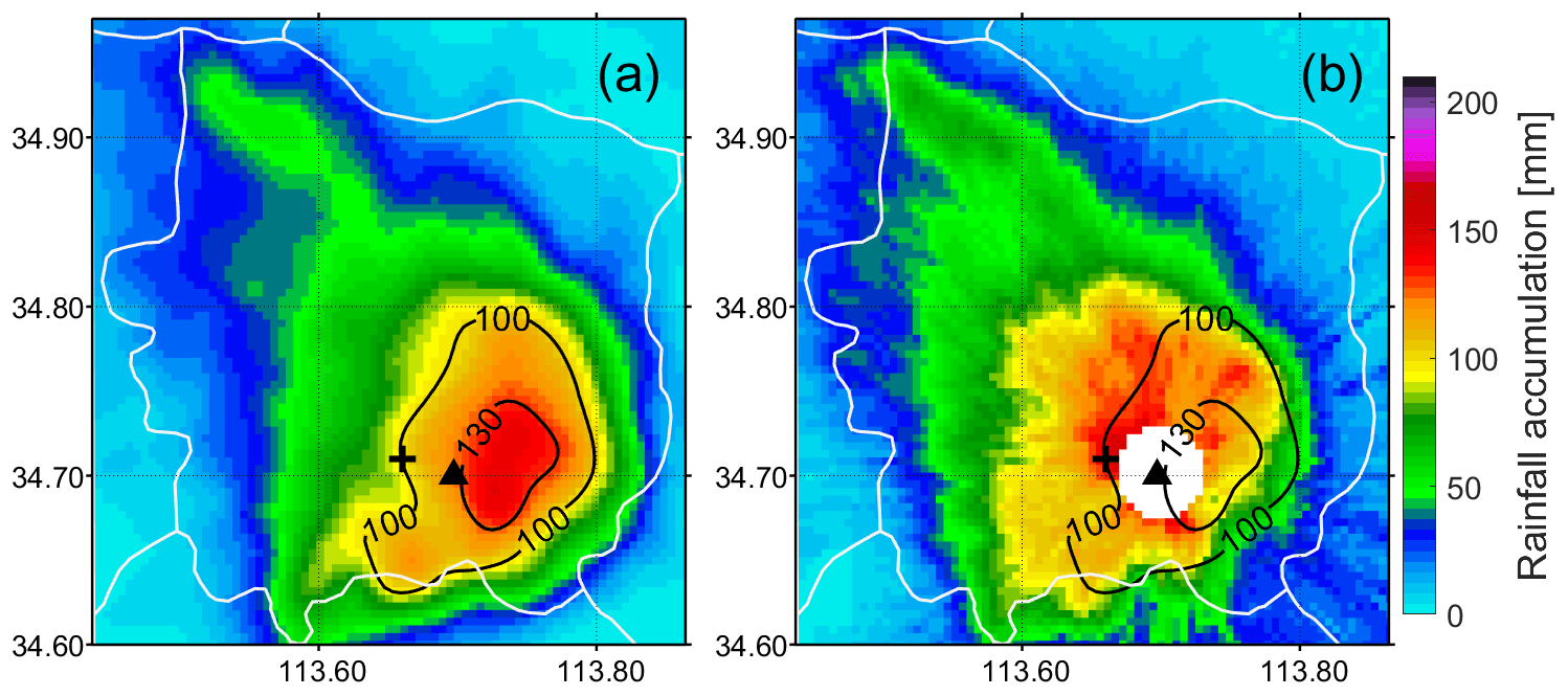
Figure 2Rainfall accumulation from 16:00 to 17:00 LST estimated using ; KDP estimates were from the operational data products (LSF method). (a) Luoyang radar data at an elevation angle of 0.5∘ and (b) Zhengzhou radar data at an elevation angle of 1.5∘ were used for comparison. Note that KDP estimates within 3 km of the Zhengzhou radar site were removed. The black triangle and cross denote the Zhengzhou radar and the gauge/OTT site, respectively. The two black isolines indicate rainfall accumulation of 100 and 130 mm, respectively, observed by the Luoyang radar.
As pointed out by Bringi and Chandrasekar (2001), the accuracy of KDP-based QPE is dependent not only on the KDP estimation from radars but also on the parameterization of R(KDP). This section will address these two respective aspects.
3.1 Approaching the “best KDP estimate”
Calculation of KDP with the Maesaka and LP algorithms requires presetting the Clpf and the window length, respectively; this controls the extent of smoothing applied to ΦDP. Bringi and Chandrasekar (2001) concluded that the minimal window length required for KDP estimation decreases with precipitation intensity. Reimel and Kumjian (2021) further showed that the best KDP estimate falls within a range of values produced by varying the parameters in known-truth simulations and that the retrieved KDP is heavily dependent on the algorithm and tuning parameter employed for steep real KDP regions. In this study, the Zhengzhou national reference climatological station hosts an OTT and the gauge with the 201.9 mm h−1 report and is 3.15 km at 274∘ azimuth from the Zhengzhou radar site. KDP estimates from different algorithms using various tuning parameters over this site were compared. Here, radar observations at elevation angles of 1.5, 2.4, 3.3, and 4.3∘ were used to investigate the following two assumptions:
-
The dependence of observed KDP on the viewing angle is expected to be negligible at small radar elevation angles, i.e., smaller than 4.3∘ (Bringi and Chandrasekar, 2001).
-
Due to the strong ground clutter contamination, we discarded the data recorded at the lowest elevation angle. KDP estimates at elevation angles of 1.5, 2.4, 3.3, and 4.3∘, corresponding to respective heights of about 0.083, 0.132, 0.182, and 0.237 km over the station, were used. Given the small range of heights, we assume that the real KDP values over Zhengzhou station at these elevation angles were about the same.
Bearing the above considerations in mind, KDP estimates using the Maesaka and LP algorithms are presented in Fig. 3. Interestingly, our results resemble those presented in Fig. 16 of Reimel and Kumjian (2021) with respect to the following aspects:
-
A stronger dependence of KDP on the tuning parameter is found for the LP algorithm than for the Maesaka algorithm.
-
The smaller window length used in the LP method generally leads to higher KDP values for heavy-rainfall periods. In comparison, KDP does not significantly change when varying Clpf from 100 to 104 for the Maesaka algorithm.
-
LP can produce higher KDP values than the Maesaka algorithm.
-
In the presence of relatively light rainfall, such as before 15:00 LST, the longer window length in LP agrees better with the Maesaka algorithm.
-
KDP values retrieved from both the LSF and Maesaka algorithms are less uncertain than LP.
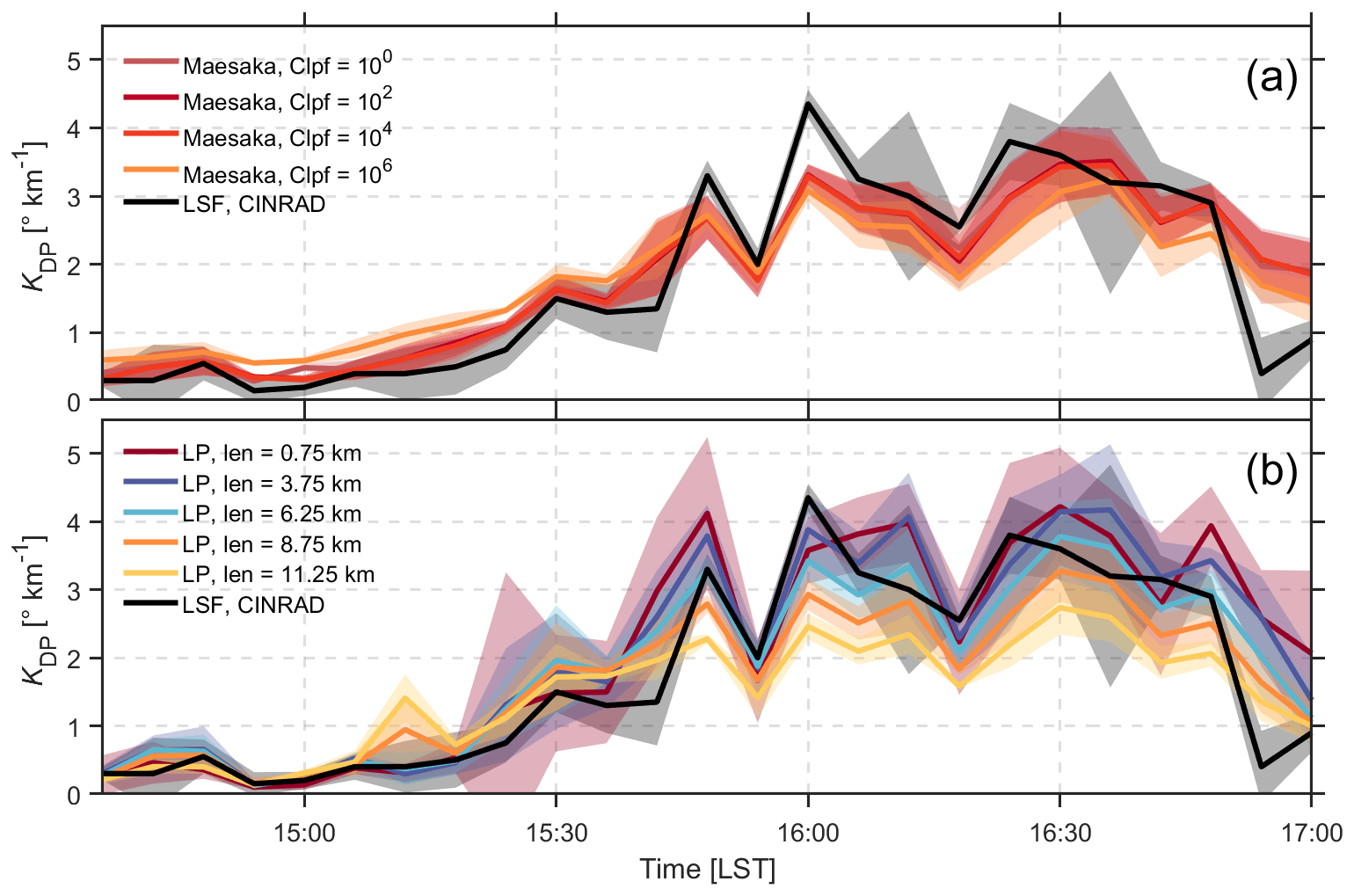
Figure 3KDP estimates using (a) the Maesaka (2012) method and (b) LP over the Zhengzhou national reference climatological station. Thick lines and shaded areas indicate the respective median values and standard deviations of KDP at elevation angles of 1.5, 2.4, 3.3, and 4.3∘. LP represents the linear programming method (Giangrande et al., 2013); LSF represents least squares fitting, which is the operational algorithm for CINRAD. Colored lines indicate the different window length (len) values used in LP.
However, the impact of changing the window length does not seem to be as significant as in Reimel and Kumjian (2021). The KDP values with a window length of 0.75 km, which is expected to yield nearly the most extreme KDP (Reimel and Kumjian, 2021), are comparable with the window length of 3.75 km (Fig. 3b). Thus, it appears that the KDP estimated using the LP algorithm has reached “saturation” at the window length of 3.75 km.
It should be noted that nonuniform radar beam filling was not considered in idealized known-truth tests (Reimel and Kumjian, 2021), but it can lead to local perturbation of KDP (Ryzhkov and Zrnic, 1998). As the LP and Maesaka algorithms assume a monotonic increase in ΦDP, they are expected to yield higher KDP than the LSF method if the negative radial slope of ΦDP occurs in close proximity. However, this effect does not seem to be significant in this study for the following reasons: the Zhengzhou radar is close to the gauge site (3.15 km), and the radar sampling volume is, therefore, much smaller than that at larger distances; the gauge site was not located on the edges of rain cells (see merged KDP observations at https://github.com/HaoranLiHelsinki/Figs_Zhengzhou, last access: 7 March 2023); and we manually checked ΦDP observations but did not see significant negative radial slope of ΦDP. Moreover, the smallest Clpf (least smoothing) yields smaller KDP than the LSF method from 16:00 to 17:00 LST (Fig. 3a), suggesting that the selection of the KDP estimation method is more important than the effect of nonuniform radar beam filling in this study.
3.2 Parameterizations of R(KDP)
While KDP is less dependent on the DSD than other radar products, a localized R(KDP) parameterization is suggested to minimize the impact of varying DSDs (e.g., Chen et al., 2022). In this study, the OTT disdrometer observations on 20 July 2021 were used as input to PyTMatrix (Leinonen, 2014) to calculate radar polarimetric variables. Before the calculation, we removed raindrops with a velocity more than ±50 % the empirical relations (Atlas et al., 1973) or with a volume equivalent diameter higher than 6 mm. It was assumed that raindrops are oblate spheroids with an aspect ratio parameterized by the equivolumetric spherical drop diameter (Thurai et al., 2007). The water temperature was set to 20 ∘C, and the orientation of rain drops was assumed to be normally distributed with a zero mean and a certain value of standard deviation (σ). We discuss the factors affecting the accuracy of R(KDP) parameterization in the following:
-
DSD. Zhang et al. (2022) showed that, for a given KDP, the fitted relation for OTT observations during the period from 16:00 to 17:00 LST yields higher precipitation rates than that for the whole day, but the difference does not exceed ∼15 mm h−1. In addition, most rain rates above 200 mm h−1 are found from 16:00 to 17:00 LST, and they follow the fitted curves rather well. Therefore, we have used the OTT data from 00:00 to 24:00 LST on 20 July 2021.
-
Assumed σ. The simulated radar polarimetric variables are dependent on σ if hydrometeors are assumed to be spheroids (Li et al., 2018). Bringi et al. (2008) found a σ of around 7∘ for a stratiform rainfall event under low-wind conditions and of 12∘ under moderate-wind conditions. In the presence of high winds, this value can be 13.6–24.7∘ (Bolek and Testik, 2022). The automatic weather station at the OTT site reported that the wind speed during this event ranged from 2 to 5 m s−1 with a peak of 7.8 m s−1 at around 16:00 LST. The magnitude of the wind speed seems rather close to the condition corresponding to a σ of 13.6∘ (Bolek and Testik, 2022).
For a given KDP of 5∘ km−1, the estimated rain rates are 203.6 and 183.6 mm h−1 for a σ of 13.6 and 7∘, respectively. This value can even be 279.4 mm h−1 (; not shown) for a σ of 24.7∘, which was observed during a tornadic squall-line storm (Bolek and Testik, 2022) and seems to be unrealistically large in this case.
-
Aspect ratio parameterization. Assuming light-wind conditions (σ=7∘), the Pruppacher and Beard (1970) and Beard and Chuang (1987) parameterizations lead to quite different rain rate estimations (Fig. 4), as earlier shown by Bringi and Chandrasekar (2001). Thurai et al. (2007) showed that the observed raindrop shapes are rather close to the model simulations in Beard and Chuang (1987). This is why we employed the Thurai et al. (2007) aspect ratio parameterization in our KDP calculations.
As shown in Fig. 4, the deviation between different parameterizations seems relatively small for smaller rain rates, but it significantly enlarges as the precipitation intensity increases. This indicates that a single R(KDP) parameterization is applicable for QPE of moderate rainfall. For higher rain rates, the fitted relation for a σ of 13.6∘ agrees rather well with Beard and Chuang (1987) and Huang et al. (2018).
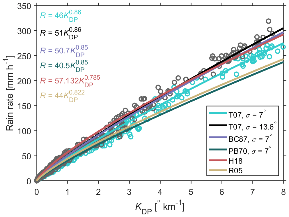
Figure 4T-matrix-based simulation of KDP vs. rain rate from the OTT observations on 20 July 2021. Black and green circles indicate observations with σ=7 and 13.6∘, respectively, assuming the aspect ratio parameterization of Thurai et al. (2007, T07). The R(KDP) relations from Ryzhkov et al. (2005, R05), Huang et al. (2018, H18), and Bringi and Chandrasekar (2001) with aspect ratio parameterizations from Pruppacher and Beard (1970, PB70) and Beard and Chuang (1987, BC87) are also presented.
3.3 Merging Zhengzhou radar observations at multiple elevation angles
One of the major challenges of using weather radar observations is to mitigate the ground clutter contamination in the vicinity of radar sites. To remove pixels affected by ground clutter, in a first step, a threshold of ρhv=0.8 (Kumjian, 2013) was implemented . Second, based on the assumption that the rain microphysics within 0.6 km of the surface do not change, the median of the radar observations at elevation angles from 0.5 to 4.3∘ was used to replace the pixels identified as ground clutter. Because of the rapid increase in the beam height at higher elevation angles, the maximum radar range decreases with increasing elevation angle for a given height. Due to clutter contamination, very few radar observations in the vicinity of the radar site at an elevation angle of 0.5∘ were used in the data merge. Meanwhile, radar data at 6.0, 9.9, 14.6, and 19.5∘ were discarded due to the limited valid data available and the fact that the elevation dependence of polarimetric measurements may start appearing (Bringi and Chandrasekar, 2001). Finally, the inverse distance weighting (IDW) interpolation (Cressman, 1959; Goudenhoofdt and Delobbe, 2009) of the radar data was applied to fill in empty regions, and the newly constructed radar data were interpolated to a spatial resolution of 0.5 km using Py-ART (Helmus and Collis, 2016).
4.1 KDP-based QPE over the gauge/OTT site
Using a parameterized R(KDP), we were able to quantitatively analyze the performance of KDP-based QPE over the gauge site. Given the high rain rates during this event, KDP estimates using the LSF method, the Maesaka algorithm with Clpf=100, and the LP method with a window length of 0.75 km are used for comparison. As shown in Fig. 5a and b, R(KDP) generally agrees well with the gauge and OTT observations before 16:00 LST, regardless of the KDP estimation method or the R(KDP) parameterizations used.
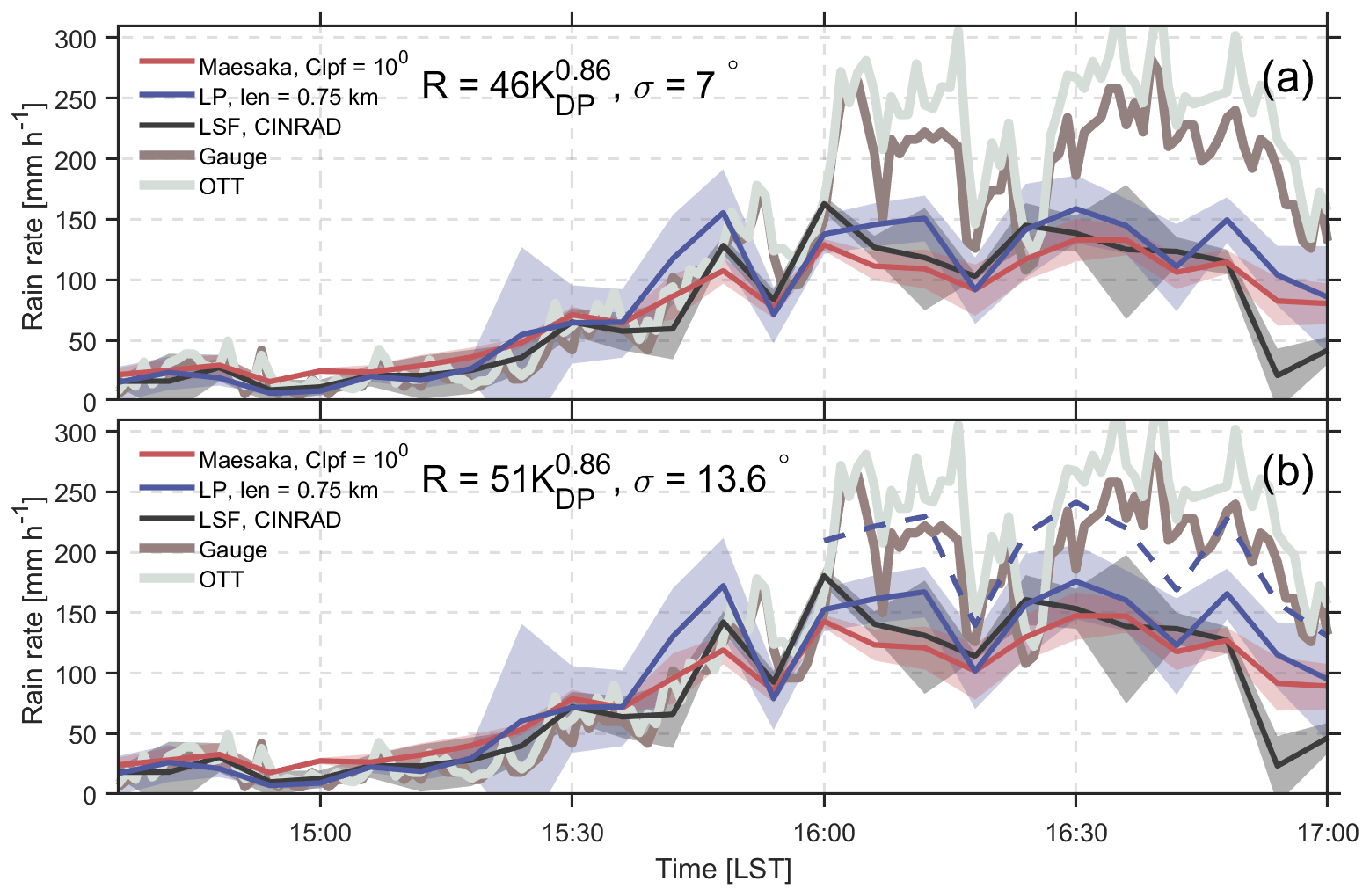
Figure 5Comparison of rainfall estimates using KDP estimated via different methods over the Zhengzhou national reference climatological station. Thick lines and shaded areas indicate the respective median values and standard deviations of rain rates estimated from KDP at elevation angles of 1.5, 2.4, 3.3, and 4.3∘. The parameterizations used are (a) and (b) . The dashed line in panel (b) presents the use of (σ=24.7∘) for QPE from 16:00 to 17:00 LST.
From 16:00 to 17:00 LST, significant deviations can be found between the gauge and OTT observations. In addition, KDP-based QPE significantly underestimates the surface precipitation during this period. With a larger σ (Fig. 5b), R(KDP) is still well below OTT/gauge observations. Therefore, it is necessary to discuss factors potentially contributing to this underestimation, which are as follows:
-
The accuracy of KDP estimates. Compared with the LSF and Maesaka algorithms, KDP estimated via the LP method underestimates the rainfall less. Note that the parameterizations used for the Maesaka and LP algorithms are expected to generate the highest KDP values for heavy rainfall (Reimel and Kumjian, 2021). Therefore, we should have good confidence that the best KDP should be close to or lower than the estimates.
-
DSD variations in the air. The lowest radar sampling volume is 0.083 km over the gauge/OTT site (1.5∘), whereas the highest radar sampling volume is 0.237 km (4.3∘). If the DSDs had varied significantly, KDP estimates at different elevation angles should also have changed. However, the uncertainty in the KDP estimates at different elevations angles is of the order of 0.5∘ km−1. Therefore, the change in DSDs should not be significant, and the DSDs observed by OTT should be applicable to radar observations that are so close to the surface. In addition, the rainwater content does not seem to change within such a short distance (Chen et al., 2020).
-
Vertical air motion. The KDP-based QPE assumes the absence of vertical air motion. For a given DSD in the radar sampling volume, downdrafts can lead to an underestimation of rain rates. For such heavy rainfall, a downdraft of 2–3 m s−1 can lead to a rain rate underestimation of 30 %–40 %. We have examined this factor from two aspects. Firstly, we found that the diameter–velocity diagram generated by OTT observations agrees rather well with the empirical relation, suggesting the absence of significant downdrafts near the surface (Kim and Song, 2018). Then, although direct retrieval of vertical air motion is rather uncertain (Oue et al., 2019) compared with the magnitude of expected downdrafts (1–2 m s−1) as shown in model simulations (Yin et al., 2022), the existence of downdrafts is detectable in the radial divergence (Roberts and Wilson, 1989; Adachi et al., 2016).
Here, we define the radial divergence (RD) as
where Vi is the observed radar Doppler velocity at the range gate ri. The RD is derived every 2 km for a range resolution of 0.25 km according to Eq. (1). Figure 6 shows time series of the observed Doppler velocity (black) as well as the RD (red) over the Zhengzhou national reference climatological station. The leading edge of the extreme-rainfall-producing storms passed the site at about 15:36 LST; during this time the Doppler velocity underwent a transition from positive to negative and the RD reached a local minimum ( s−1), indicating the presence of updrafts. From 16:00 to 17:00 LST, the Doppler velocity is around 0 m s−1 and RD is about s−1, suggesting sustained downdrafts. Therefore, unquantified downward air motion may be responsible for the underestimation of rainfall accumulation.
-
The assumption of σ. As shown in Fig. 4, the assumption of σ is critical for the parameterization of R(KDP). However, σ cannot be measured by OTT, and very few experiments have been conducted to address this issue (e.g., Bringi et al., 2008; Bolek and Testik, 2022). The wind observations are rather close to what was reported by Bolek and Testik (2022), and σ=13.6∘ seems to be a good first guess. If the σ=24.7∘ measured during the passage of a tornadic squall-line storm (the 4 min running average horizontal wind speed is 6–10 m s−1) is used, the resulting rain rate estimation is rather close to gauge/OTT measurements (dashed line in Fig. 5b). However, the observed horizontal wind speed is 3–5 m s−1 from 16:00 to 17:00 LST (Fig. 1d). Therefore, even though we cannot give a more accurate estimate of σ, 24.7∘ seems to be unrealistically large in this study.
-
Different sampling volumes between the radar and the gauge/OTT. The width of the sampling volume for the Zhengzhou radar with a beam width of 1∘ over the gauge site is about 55 m, which is much larger than that of a gauge. Although this effect is difficult to quantify, we argue that it plays a minor role in the rainfall underestimation. By manually checking the movement of storms (merged KDP observations at https://github.com/HaoranLiHelsinki/Figs_Zhengzhou, last access: 7 March 2023), we found that the storm propagation speed is of the order of several kilometers per hour, contrasting with the much smaller radar sampling volume. Given the rapidly changing nature of storms, the sampling effect does not seem to be a major factor responsible for rainfall underestimation.
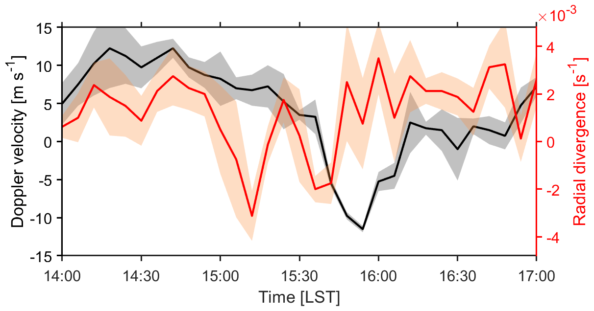
Figure 6Doppler velocity (left axis) and radial divergence (right axis) observed over the Zhengzhou national reference climatological station. Thick lines and shaded areas indicate the respective median values and standard deviations at elevation angles of 1.5, 2.4, 3.3, and 4.3∘.
4.2 Statistical evaluation
The dense meteorological and hydrological rain gauge network in Zhengzhou city allows for statistical evaluation of the KDP-based QPE. In addition, R(KDP) is expected to be less uncertain than other approaches for heavy precipitation (Ryzhkov et al., 2022). Therefore, the performance of R(KDP) during the most intense precipitation period (14:00–17:00 LST) was investigated. As discussed above, the assumption of σ=13.6∘ appears to be more suitable than the commonly used 7∘ for this event; thus, was used. Note that the gridded R(KDP), as introduced in Sect. 3.3, was used for comparison.
For rainfall rates below 50 mm h−1, the standard deviation (SD) and bias of R(KDP) are mostly of the order of 7–8 mm h−1 and −1 to 0 mm h−1, respectively. Regarding the LP method, the window length used does not significantly degrade the accuracy of QPE (Fig. 7a, b, c, d, e). The performance of the Maesaka method is comparable to that of the LP method (Fig. 7f, g, h), except for Clpf=106 (Fig. 7i) which imposes an overly aggressive filter that obviously leads to oversmoothing as well as a much larger SD and bias. The operationally used LSF method (Fig. 7j) shows relatively large bias values (1.8 mm h−1), indicating that the KDP derived using the LSF method for rainfall rates below 50 mm h−1 should be used with caution.
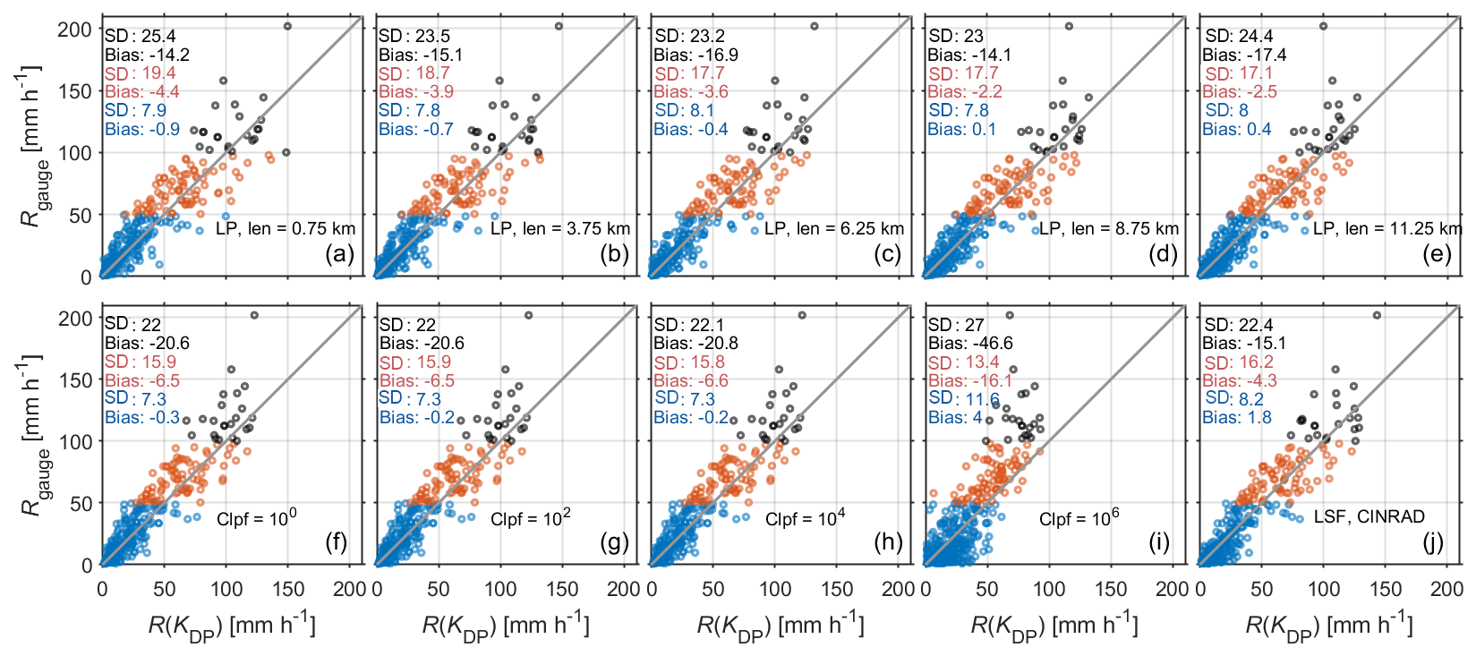
Figure 7KDP-based hourly rainfall accumulation vs. gauge observations from 14:00 to 17:00 LST. KDP was estimated using the (a–e) LP, (f–i) Maesaka, and (j) LSF methods. Rain rates were divided into three groups: Rgauge<50 mm h−1 (blue), 50 mm h mm h−1 (red), and 100 mm h (black). The standard deviation (SD) and bias between Rgauge and R(KDP) for each group are marked using the corresponding colors. was used.
For rainfall rates above 50 mm h−1, R(KDP) generally underestimates hourly rainfall accumulation, and this underestimation becomes more significant as the rain rate increases (smaller bias and SD values for the red dots than for the black dots). KDP values estimated using the Maesaka algorithm are smaller on average than those estimated using the LP and LSF methods, which is consistent with the results in Fig. 3. Interestingly, the SD and bias of the LP method are very close to those of the LST method, regardless of the used window length. This indicates that varying the window length from 0.75 to 11.25 km has minimal impact on the accuracy of R(KDP) for rain rates of 50 to ∼100 mm h−1 for this event.
Reimel and Kumjian (2021) showed that smaller a window length employed in the LP method yields higher KDP. This appears to be true for the gauge with the 201.9 mm h−1 report, but decreasing the window length did not significantly ameliorate the underestimation from a statistical perspective (Fig. 7a, b, c, d, e). Specifically, the highest hourly rainfall accumulation was found for the LP method, and the value rose from 100 mm h−1 (len=11.25 km) to 149.6 mm h−1 (len=0.75 km). For reference, the value was 122.9 and 143.3 mm h−1 for the Maesaka method with Clpf=100 and for the LSF method, respectively.
As discussed above, the use of the window length (LP method) and Clpf (Maesaka algorithm) has limited impact on heavy-rainfall QPE, and a window length of 0.75 km generates the closest rainfall estimation to the 201.9 mm h−1 report. Therefore, we have compared the areal hourly rainfall accumulation based on KDP values generated using these three methods during the period with most intense rainfall (14:00–17:00 LST).
As shown in Fig. 8, the rainfall rate hot spots can be manually identified, and the results of the three methods generally agree with each other for R(KDP)<100 mm h−1. However, an in-depth analysis reveals that the magnitudes of the rainfall accumulation are different at higher rain rates. From 16:00 to 17:00 LST (Fig. 8a3, 8b3, 8c3), the rainfall hot spots are in the vicinity of the Zhengzhou radar site (black triangle Fig. 8). The LP method is characterized by the largest area of R(KDP)>130 mm h−1 (Fig. 8a3), whereas the smallest area is found for the Maesaka algorithm (Fig. 8b3). However, due to the scarcity of gauges in the area of rainfall hot spots, this difference is noticeable only for the gauge with the 201.9 mm h−1 report (black cross Fig. 8).
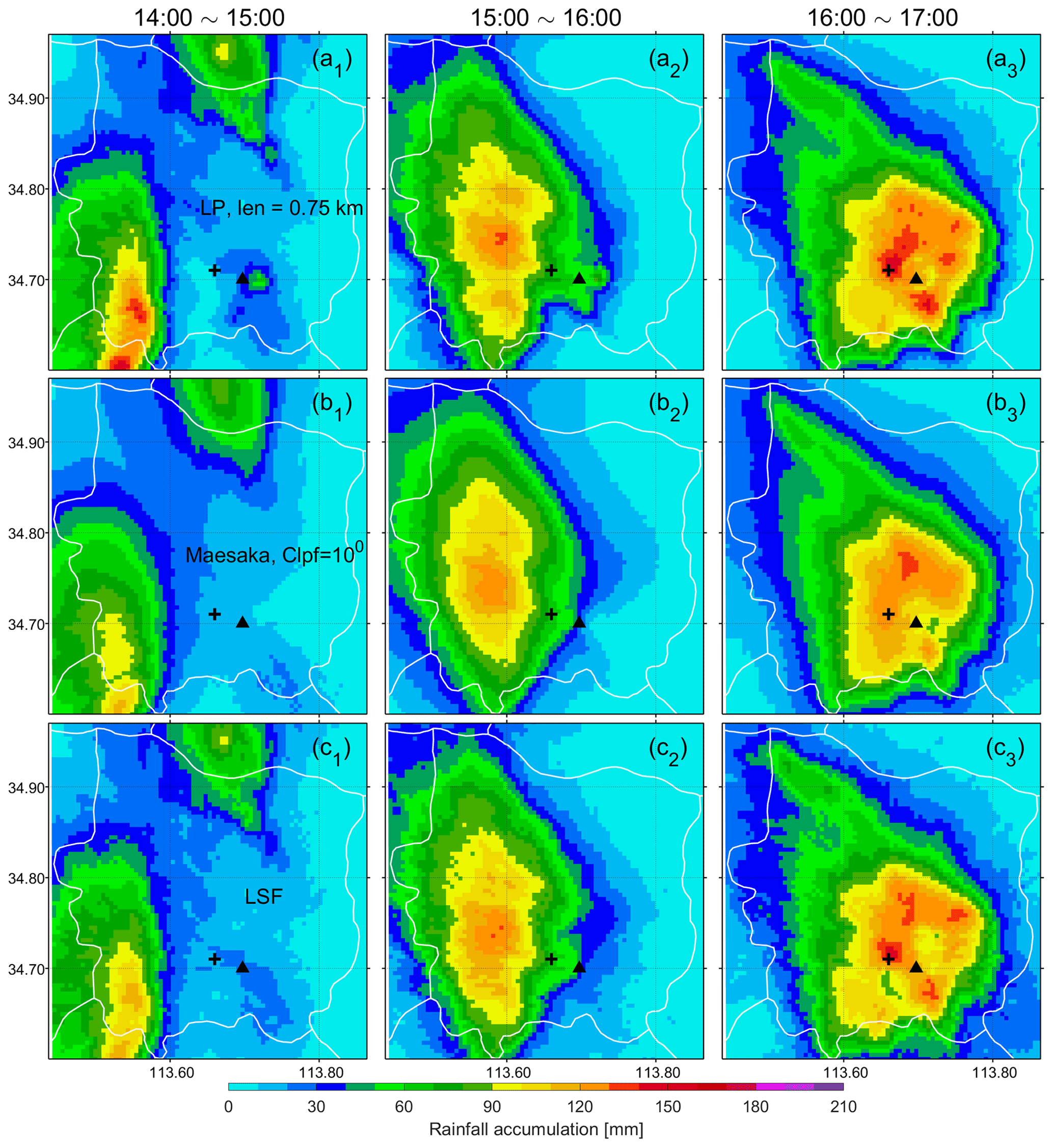
Figure 8Hourly areal rainfall map from 14:00 to 17:00 LST. KDP was estimated using (a) the LP method with LP=0.75 km, (b) the Maesaka method with Clpf=100, and (c) the LSF method. The black triangle and cross denote the Zhengzhou radar and the site hosting the gauge with the 201.9 mm h−1 report, respectively. was used.
The areal hourly rainfall accumulation enables the analysis of the evolution of this event. As shown in Fig. 8a, the precipitation system moved into Zhengzhou city from the southwest causing rainfall of up to 130 mm h−1 from 14:00 to 15:00 LST (Fig. 8a). It then slowly propagated northeastward over the next hour with increased precipitation intensity. Hourly rainfall of more than 100 mm h−1 covered a north–south oriented, ellipse-shaped area of about 115.5 km2. From 16:00 to 17:00 LST, the precipitation system moved eastward, causing the most intense hourly rainfall over the center of Zhengzhou city (Fig. 8c). A rainfall rate of more than 100 mm h−1 was observed over an area of about 198.25 km2, which was 171.7 % that of the previous 1 h. The increased rainfall extremity and the more localized extreme rainfall likely resulted from the mergence of convective cells and the formation of an arc-shaped convergence zone that favored the development of convective updrafts in a three-quarter circle around the storm (Yin et al., 2022). Interestingly, the gauge with the 201.9 mm h−1 report was located almost exactly in the high-value center of the hourly rainfall map at 17:00 LST.
The accumulated rainfall from 14:00 to 17:00 LST is presented in Fig. 9. As expected, the results of the LP method and the LSF method are similar, whereas the area of rainfall accumulation exceeding 200 mm generated by the Maesaka method is significantly different from those using the other two methods. Interestingly, we have found that the center of the 3 h rainfall accumulation was offset with respect to the hot spot encompassing the record-breaking hourly rainfall accumulation (16:00–17:00 LST; Fig. 8a3). Specifically, the center of the 3 h rainfall accumulation was located southwest of Zhengzhou city, which is fortunately an urban–rural fringe area where the surface is less impervious and in which relatively fewer residents were living.
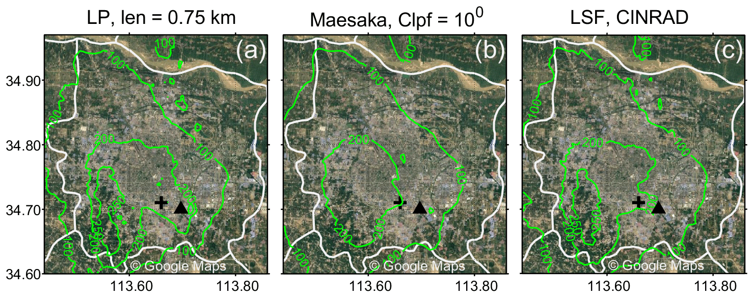
Figure 9Satellite images from Google Maps overlaid with isolines indicating the rainfall accumulation (mm) during the 14:00–17:00 LST period. The rain rate was inferred from ; KDP was estimated using (a) the LP method with len=0.75 km, (b) the Maesaka algorithm with Clpf=100, and (c) the LSF method. The black triangle and cross denote the Zhengzhou radar and the site hosting the gauge with the 201.9 mm h−1 report, respectively.
In this study, we examined KDP-based QPE for the record-breaking extreme-rainfall event that occurred over Zhengzhou between 14:00 and 17:00 LST on 20 July 2021. The rain DSD observations obtained using an OTT disdrometer were used to develop R(KDP) parameterizations. The KDP estimates generated via the operationally used LSF method were compared with two parameter-controlled methods. The KDP estimates were gridded with a spatial resolution of 500 m, and the results of R(KDP) were compared with gauge observations. The results can be summarized as follows:
-
The range degradation effect significantly affected the performance of radar-based QPE for this event. The precipitation center as identified by the Luoyang radar – about 120 km from the Zhengzhou city center – significantly deviated from the Zhengzhou radar estimates.
-
The assumed σ in the T-matrix simulation has a tangible impact on the development of R(KDP) parameterizations. A higher σ value results in a smaller KDP in simulations for a given rain DSD. The previous experimental study by Bringi et al. (2008) on σ was undertaken under low-wind conditions; thus, the applicability of the σ assumption under moderate- to strong-wind conditions should be addressed in future studies.
-
Gauges deployed over Zhengzhou city were used to evaluate the accuracy of R(KDP). The results show that all methods agree with each other rather well for R(KDP)<100 mm h−1. The LP method is capable of producing the highest rainfall accumulation. In a statistical sense, changing the window length from 0.75 to 11.25 km in the LP method or changing Clpf from 100 to 104 in the Maesaka algorithm does not significantly affect the QPE performance; moreover, oversmoothing was found for the Maesaka algorithm with Clpf=106.
-
The KDP estimates from the three algorithms for the region comprising the gauge with the 201.9 mm h−1 report were compared, and the results are generally similar to Reimel and Kumjian (2021). One notable difference is that the estimated KDP almost reached “saturation” at a window length of 3.75 km, and the increase in KDP with a decrease in window length is not as significant as that in Reimel and Kumjian (2021). The results of the LP method with a window length of 0.75 km are close to those of the LSF method but significantly larger than the highest values obtained from the Maesaka algorithm.
-
R(KDP) with the KDP estimation using the three methods cannot reproduce the gauge-observed value of 201.9 mm h−1. Our comparisons suggest that this underestimation is unlikely due to the KDP estimation process; rather, the adequacy of the assumed σ and unquantified vertical air motion may explain the underestimation.
-
The gauge with the 201.9 mm h−1 report was located in the vicinity of local rainfall hot spots during the period from 16:00 to 17:00 LST, but the center of the 3 h areal rainfall accumulation was found to be located to the southwest of Zhengzhou city, deviating from the site with the 201.9 mm h−1 record.
From the perspective of operational applications, the effect of smoothing on KDP estimation is interesting. Our results show that the use of a smoothing factor has minimal impact on KDP for hourly rainfall accumulation below 100 mm; however, its impact becomes more significant as the rain rate increases. This suggests the importance of employing an adaptive window length, as used in the LSF method. However, the current LP and Maesaka algorithms use a fixed window length or a single smoothing factor, respectively. The future development of a new LP algorithm with an adaptive window length is recommended. In addition, we speculate that the underestimation of the 201.9 mm h−1 rainfall accumulation value can be attributed to inadequate assumptions about raindrop microphysics and unquantified vertical air motion. Although we cannot quantify their contributions during the Zhengzhou event, more focused observational experiments are suggested to ascertain their impact on radar-based QPE.
Extreme-rainfall events are relatively rare, but they are very destructive. We call for integrated efforts to tackle the issue of radar data quality control as well as to promote the capability of operational weather radars in extreme-rainfall monitoring. This will improve hydrological modeling, extreme-rainfall nowcasting, and disaster mitigation for cities, and it will also be valuable to studies of mechanisms governing extreme rainfall production.
The data used in this study can be accessed by contacting the first author. The merged KDP figures are available from https://doi.org/10.5281/zenodo.7703316 (Li, 2023). The hourly QPE products generated in this study are available from https://doi.org/10.5281/zenodo.7703316 (Li, 2023).
HL and DM conceptualized the study. HL performed the experiment and wrote the paper. All authors took part in the interpretation of the results and edited the manuscript.
The contact author has declared that none of the authors has any competing interests.
Publisher's note: Copernicus Publications remains neutral with regard to jurisdictional claims in published maps and institutional affiliations.
This article is part of the special issue “Attributing and quantifying the risk of hydrometeorological extreme events in urban environments”. It is not associated with a conference.
We thank Scott Giangrande, Zhe Zhang, and Tanel Voormansik for helpful discussions on the linear programming method.
This research has been supported by the National Natural Science Foundation of China (grant nos. 42030610, 41975046 and U2142210) and the Chinese Academy of Meteorological Sciences' Basic Research and Operation Fund (grant no. 451490).
Open-access funding was provided by the Helsinki University Library.
This paper was edited by Patrick Laux and reviewed by three anonymous referees.
Adachi, T., Kusunoki, K., Yoshida, S., Arai, K.-I., and Ushio, T.: High-speed volumetric observation of a wet microburst using X-band phased array weather radar in Japan, Mon. Weather Rev., 144, 3749–3765, 2016. a
Allan, R. P. and Soden, B. J.: Atmospheric warming and the amplification of precipitation extremes, Science, 321, 1481–1484, 2008. a
Atlas, D., Srivastava, R., and Sekhon, R. S.: Doppler radar characteristics of precipitation at vertical incidence, Rev. Geophys., 11, 1–35, 1973. a
Beard, K. V. and Chuang, C.: A new model for the equilibrium shape of raindrops, J. Atmos. Sci., 44, 1509–1524, 1987. a, b, c, d
Bolek, A. and Testik, F. Y.: Rainfall Microphysics Influenced by Strong Wind during a Tornadic Storm, J. Hydrometeorol., 23, 733–746, https://doi.org/10.1175/JHM-D-21-0004.1, 2022. a, b, c, d, e
Bringi, V., Thurai, M., and Brunkow, D.: Measurements and inferences of raindrop canting angles, Electron. Lett., 44, 1425–1426, 2008. a, b, c
Bringi, V. N. and Chandrasekar, V.: Polarimetric Doppler weather radar: principles and applications, Cambridge University Press, ISBN 0-521-62384-7, 2001. a, b, c, d, e, f
Bruni, G., Reinoso, R., van de Giesen, N. C., Clemens, F. H. L. R., and ten Veldhuis, J. A. E.: On the sensitivity of urban hydrodynamic modelling to rainfall spatial and temporal resolution, Hydrol. Earth Syst. Sci., 19, 691–709, https://doi.org/10.5194/hess-19-691-2015, 2015. a
Chen, B., Yang, J., Gao, R., Zhu, K., Zou, C., Gong, Y., and Zhang, R.: Vertical variability of the raindrop size distribution in typhoons observed at the Shenzhen 356-m meteorological tower, J. Atmos. Sci., 77, 4171–4187, 2020. a
Chen, F.-W. and Liu, C.-W.: Estimation of the spatial rainfall distribution using inverse distance weighting (IDW) in the middle of Taiwan, Paddy Water Environ., 10, 209–222, 2012. a
Chen, G., Zhao, K., Lu, Y., Zheng, Y., Xue, M., Tan, Z.-M., Xu, X., Huang, H., Chen, H., Xu, F., and Yang, J.: Variability of microphysical characteristics in the “21⋅7” Henan extremely heavy rainfall event, Sci. China Earth Sci., 65, 1861–1878, 2022. a
Cremonini, R., Voormansik, T., Post, P., and Moisseev, D.: Estimation of extreme precipitations in Estonia and Italy using dual-pol weather radar QPEs, Atmos. Meas. Tech. Discuss. [preprint], https://doi.org/10.5194/amt-2022-220, in review, 2022. a, b
Cressman, G. P.: An operational objective analysis system, Mon. Weather Rev., 87, 367–374, 1959. a
Ding, Y.: The major advances and development of the theory on heavy rains in China, Torrential Rain and Disasters, 38, 395–406, 2019. a
Donat, M. G., Lowry, A. L., Alexander, L. V., O'Gorman, P. A., and Maher, N.: More extreme precipitation in the world's dry and wet regions, Nat. Clim. Change, 6, 508–513, 2016. a
Giangrande, S. E., McGraw, R., and Lei, L.: An Application of Linear Programming to Polarimetric Radar Differential Phase Processing, J. Atmos. Ocea. Tech., 30, 1716–1729, https://doi.org/10.1175/JTECH-D-12-00147.1, 2013. a, b, c
Goudenhoofdt, E. and Delobbe, L.: Evaluation of radar-gauge merging methods for quantitative precipitation estimates, Hydrol. Earth Syst. Sci., 13, 195–203, https://doi.org/10.5194/hess-13-195-2009, 2009. a
Helmus, J. J. and Collis, S. M.: The Python ARM Radar Toolkit (Py-ART), a library for working with weather radar data in the Python programming language, J. Open Res. Softw., 4, e25, https://doi.org/10.5334/jors.119, 2016. a, b, c, d
Huang, H., Zhao, K., Zhang, G., Lin, Q., Wen, L., Chen, G., Yang, Z., Wang, M., and Hu, D.: Quantitative Precipitation Estimation with Operational Polarimetric Radar Measurements in Southern China: A Differential Phase-Based Variational Approach, J. Atmos. Ocean. Tech., 35, 1253–1271, https://doi.org/10.1175/JTECH-D-17-0142.1, 2018. a, b
Kim, D.-K. and Song, C.-K.: Characteristics of vertical velocities estimated from drop size and fall velocity spectra of a Parsivel disdrometer, Atmos. Meas. Tech., 11, 3851–3860, https://doi.org/10.5194/amt-11-3851-2018, 2018. a
Kumjian, M. R.: Principles and Applications of Dual-Polarization Weather Radar. Part I: Description of the Polarimetric Radar Variables, J. Oper. Meteorol., 1, 226–242, https://doi.org/10.15191/nwajom.2013.0119, 2013. a
Lang, T. J., Nesbitt, S. W., and Carey, L. D.: On the correction of partial beam blockage in polarimetric radar data, J. Atmos. Ocean. Tech., 26, 943–957, 2009. a
Leinonen, J.: High-level interface to T-matrix scattering calculations: architecture, capabilities and limitations, Opt. Express, 22, 1655–1660, 2014. a
Li, H.: Assessing specific differential phase (KDP)-based quantitative precipitation estimation for the record-breaking rainfall over Zhengzhou city on 20 July 2021, Zenodo [data set], https://doi.org/10.5281/zenodo.7703316, 2023. a, b
Li, H., Moisseev, D., and von Lerber, A.: How does riming affect dual-polarization radar observations and snowflake shape?, J. Geophys. Res.-Atmos., 123, 6070–6081, 2018. a
Liu, X., He, B., Zhao, S., Hu, S., and Liu, L.: Comparative measurement of rainfall with a precipitation micro-physical characteristics sensor, a 2D video disdrometer, an OTT PARSIVEL disdrometer, and a rain gauge, Atmos. Res., 229, 100–114, 2019. a
Luo, Y., Sun, J., Li, Y., Xia, R., Du, Y., Yang, S., Zhang, Y., Chen, J., Dai, K., Shen, X., Chen, H., Zhou, F., Liu, Y., Fu, S., Wu, M., Xiao, T., Chen, Y., Li, H., and Li, M.: Science and prediction of heavy rainfall over China: Research progress since the reform and opening-up of new China, J. Meteorol. Res., 34, 427–459, 2020. a
Maesaka, T., Iwanami, K., and Maki, M.: Non-negative KDP estimation by monotone increasing ΦDP assumption below melting layer, in: Extended Abstracts, in: vol. 3, Seventh European Conf. on Radar in Meteorology and Hydrology, 3 June 2012, Toulouse, France, 2012. a, b
Oue, M., Kollias, P., Shapiro, A., Tatarevic, A., and Matsui, T.: Investigation of observational error sources in multi-Doppler-radar three-dimensional variational vertical air motion retrievals, Atmos. Meas. Tech., 12, 1999–2018, https://doi.org/10.5194/amt-12-1999-2019, 2019. a
Park, S.-G., Kim, H.-L., Ham, Y.-W., and Jung, S.-H.: Comparative evaluation of the OTT PARSIVEL 2 using a collocated two-dimensional video disdrometer, J. Atmos. Ocean. Tech., 34, 2059–2082, 2017. a
Paz, I., Tchiguirinskaia, I., and Schertzer, D.: Rain gauge networks’ limitations and the implications to hydrological modelling highlighted with a X-band radar, J. Hydrol., 583, 124615, https://doi.org/10.1016/j.jhydrol.2020.124615, 2020. a
Pruppacher, H. R. and Beard, K.: A wind tunnel investigation of the internal circulation and shape of water drops falling at terminal velocity in air, Q. J. Roy. Meteorol. Soc., 96, 247–256, 1970. a, b
Reimel, K. J. and Kumjian, M.: Evaluation of KDP estimation algorithm performance in rain using a known-truth framework, J. Atmos. and Ocean. Tech., 38, 587–605, 2021. a, b, c, d, e, f, g, h, i, j, k, l, m, n
Roberts, R. D. and Wilson, J. W.: A proposed microburst nowcasting procedure using single-Doppler radar, J. Appl. Meteorol. Clim., 28, 285–303, 1989. a
Ryzhkov, A. and Zrnic, D.: Beamwidth effects on the differential phase measurements of rain, J. Atmos. Ocean. Tech., 15, 624–634, 1998. a
Ryzhkov, A., Zhang, P., Bukovčić, P., Zhang, J., and Cocks, S.: Polarimetric Radar Quantitative Precipitation Estimation, Remote Sens., 14, 1695, https://doi.org/10.3390/rs14071695, 2022. a, b, c
Ryzhkov, A. V., Giangrande, S. E., and Schuur, T. J.: Rainfall Estimation with a Polarimetric Prototype of WSR-88D, J. Appl. Meteorol., 44, 502–515, https://doi.org/10.1175/JAM2213.1, 2005. a
Schleiss, M., Olsson, J., Berg, P., Niemi, T., Kokkonen, T., Thorndahl, S., Nielsen, R., Ellerbæk Nielsen, J., Bozhinova, D., and Pulkkinen, S.: The accuracy of weather radar in heavy rain: a comparative study for Denmark, the Netherlands, Finland and Sweden, Hydrol. Earth Syst. Sci., 24, 3157–3188, https://doi.org/10.5194/hess-24-3157-2020, 2020. a
Schroeer, K., Kirchengast, G., and Sungmin, O.: Strong dependence of extreme convective precipitation intensities on gauge network density, Geophys. Res. Lett., 45, 8253–8263, 2018. a
Thurai, M., Huang, G., Bringi, V., Randeu, W., and Schönhuber, M.: Drop shapes, model comparisons, and calculations of polarimetric radar parameters in rain, J. Atmos. Oocean. Tech., 24, 1019–1032, 2007. a, b, c, d
Tokay, A., Petersen, W. A., Gatlin, P., and Wingo, M.: Comparison of raindrop size distribution measurements by collocated disdrometers, J. Atmos. Ocean. Tech., 30, 1672–1690, 2013. a
Trömel, S., Kumjian, M. R., Ryzhkov, A. V., Simmer, C., and Diederich, M.: Backscatter differential phase – Estimation and variability, J. Appl. Meteorol. Clim., 52, 2529–2548, 2013. a
Wang, Y. and Chandrasekar, V.: Algorithm for estimation of the specific differential phase, J. Atmos. Ocean. Tech., 26, 2565–2578, 2009. a
Yin, J., Gu, H., Liang, X., Yu, M., Sun, J., Xie, Y., Li, F., and Wu, C.: A possible dynamic mechanism for rapid production of the extreme hourly rainfall in Zhengzhou city on 20 July 2021, J. Meteorol. Res., 36, 6–25, 2022. a, b, c, d, e
Yu, S., Luo, Y., Wu, C., Zheng, D., Liu, X., and Xu, W.: Convective and Microphysical Characteristics of Extreme Precipitation Revealed by Multisource Observations Over the Pearl River Delta at Monsoon Coast, Geophys. Res. Lett., 49, e2021GL097043, https://doi.org/10.1029/2021GL097043, 2022. a
Zhang, D.-L.: Rapid urbanization and more extreme rainfall events, Sci. Bull., 65, 516–518, 2020. a
Zhang, W., Villarini, G., Vecchi, G. A., and Smith, J. A.: Urbanization exacerbated the rainfall and flooding caused by hurricane Harvey in Houston, Nature, 563, 384–388, 2018. a
Zhang, Z., Qi, Y., Li, D., Zhao, Z., Cui, L., Su, A., and Wang, X.: Raindrop Size Distribution Characteristics of the “7 20” Extreme Rainstorm Event in Zhengzhou, 2021 and its Impacts on Radar Quantitative Precipitation Estimation, Chinese J. Atmos. Sci., 46, 1002–1016, https://doi.org/10.3878/j.issn.1006-9895.2201.21237, 2022. a