Remote sensing-aided rainfall–runoff modeling in the tropics of Costa Rica

Streamflow simulation across the tropics is limited by the lack of data to calibrate and validate large-scale hydrological models. Here, we applied the process-based, conceptual HYPE (Hydrological Predictions for the Environment) model to quantitatively assess Costa Rica's water resources at a national scale. Data scarcity was compensated for by using adjusted global topography and remotely sensed climate products to force, calibrate, and independently evaluate the model. We used a global temperature product and bias-corrected precipitation from Climate Hazards Group InfraRed Precipitation with Station data (CHIRPS) as model forcings. Daily streamflow from 13 gauges for the period 1990–2003 and monthly Moderate Resolution Imaging Spectroradiometer (MODIS) potential evapotranspiration (PET) and actual evapotranspiration (AET) for the period 2000–2014 were used to calibrate and evaluate the model applying four different model configurations (M1, M2, M3, M4). The calibration consisted of step-wise parameter constraints preserving the best parameter sets from previous simulations in an attempt to balance the variable data availability and time periods. The model configurations were independently evaluated using hydrological signatures such as the baseflow index, runoff coefficient, and aridity index, among others. Results suggested that a two-step calibration using monthly and daily streamflow (M2) was a better option than calibrating only with daily streamflow (M1), with similar mean Kling–Gupta efficiency (KGE ∼ 0.53) for daily streamflow time series, but with improvements to reproduce the flow duration curves, with a median root mean squared error (RMSE) of 0.42 for M2 and a median RMSE of 1.15 for M1. Additionally, including AET (M3 and M4) in the calibration statistically improved the simulated water balance and better matched hydrological signatures, with a mean KGE of 0.49 for KGE in M3–M4, in comparison to M1–M2 with mean KGE < 0.3. Furthermore, Kruskal–Wallis and Mann–Whitney statistical tests support a similar model performance for M3 and M4, suggesting that monthly PET-AET and daily streamflow (M3) represents an appropriate calibration sequence for regional modeling. Such a large-scale hydrological model has the potential to be used operationally across the humid tropics informing decision-making at relatively high spatial and temporal resolution.

1 Introduction

Tropical regions differ from temperate regions by their larger energy inputs, more intense atmospheric dynamics, higher precipitation rates, larger streamflow, and greater sediment yields (Dehaspe et al., 2018; Esquivel-Hernández et al., 2017; Wohl et al., 2012). Moreover, tropical regions are among the fastest-changing environments, with a hydrological cycle pressurized by population growth (Wohl et al., 2012; Ziegler et al., 2007), land use/cover modifications (Gibbs et al., 2010), and altered precipitation and runoff patterns (Esquivel-Hernández et al., 2017) due to climate change. Central America, the northern boundary of the humid tropics, was identified by Giorgi (2006) as the most sensitive tropical region to climate change due to the location between two major water bodies, the Pacific Ocean and the Caribbean Sea.

Increasing concerns about the effects of human activities and climate change on tropical catchments demand accurate quantification of the water balance components in space and time to guarantee future water resources availability for ecosystems and socioeconomic activities (Esquivel-Hernández et al., 2017; Wohl et al., 2012). Hydrological models have been widely used to assess the spatiotemporal variability of water resources and to provide insights into potential future climate and management decisions (Andersson et al., 2015; Xiong and Zeng, 2019).

However, models also implicitly include many uncertainties (Beven, 2012). For example, Birkel et al. (2020) and Dehaspe et al. (2018) highlighted those hydrological models that are useful for predicting streamflow but showed limitations to assess water partitioning and storage changes required for water management in the humid tropics. Modeling in the tropics is further hampered by the lack of good quality hydrometric data used to drive models and for calibration (Westerberg and Birkel, 2015; Westerberg et al., 2014). Moreover, a decrease in hydrological measurements and monitoring networks in many tropical regions has occurred during the last 3 decades (Wohl et al., 2012), limiting the applicability of hydrological models or reducing their performance in simulating streamflow in Central America (Westerberg et al., 2014) and South America (Guimberteau et al., 2012). Model calibration mostly leads to several combinations of parameters with similar streamflow response, i.e., equifinality (Beven, 2012; Xiong and Zeng, 2019), and it is therefore desirable to reduce or constrain the uncertainty of model parameters. Moreover, some case studies around the world have found that soil model parameters can be relatively insensitive to streamflow simulations (Massari et al., 2015; Rajib et al., 2018b; Silvestro et al., 2015).

Opportunities to provide more realistic internal hydrological partitioning exist in the form of including additional variables to streamflow, such as, e.g., tracers and remotely sensed variables of evapotranspiration and soil moisture (Dal Molin et al., 2020; Rakovec et al., 2016; Xiong and Zeng, 2019; Massari et al., 2015). The latter, however, may come at the expense of increased complexity for model calibration and evaluation (Arheimer et al., 2020; Her and Seong, 2018; Massari et al., 2015; Xiong and Zeng, 2019; Zhang et al., 2018) since non-linearity increases complexity in data assimilation (Massari et al., 2015; Rajib et al., 2018a, b). In addition, hydrological signatures can improve model realism through the synthesis of many simultaneous catchment processes at different scales (Arheimer et al., 2020; Sawicz et al., 2011). Hydrological signatures can be used to increase our understanding of water balance partitioning and hydrological similarity across different scales (e.g., Arciniega-Esparza et al., 2017; Beck et al., 2015; Kirchner, 2009; Troch et al., 2009) and have been applied to improve model evaluation (e.g., Andersson et al., 2015; Arheimer et al., 2020; Dal Molin et al., 2020; Raphael Tshimanga and Hughes, 2014; Westerberg et al., 2014). Despite uncertainties in observed hydrological signatures (Westerberg and McMillan, 2015), there is potential to identify model weaknesses and to ultimately produce a more well-balanced catchment representation.

Most hydrological models have been developed since the 1970s to solve different needs at catchment scales (Pechlivanidis and Arheimer, 2015; Todini, 2007). Nevertheless, water management increasingly requires detailed hydrological information over larger, aggregated spatial domains instead of a single catchment (Arheimer et al., 2020; Rojas-Serna et al., 2016). Global hydrological models can serve this purpose but suffer from rather coarse spatial resolution and increased computational cost (Kumar et al., 2013; Sood and Smakhtin, 2015). Distributed landscape characteristics at large scales such as soil, topography, and land cover can result in complex hydrological models with many calibrated model parameters (Gurtz et al., 1999) and result in greater uncertainty. However, distributed model parameterization based on landscape characteristics also promises the advantage of predicting the hydrological response of ungauged basins (Hrachowitz et al., 2013; Pechlivanidis and Arheimer, 2015). Therefore, the question as to how complex or simple a hydrological model should be remains an open scientific debate considering that simpler models can lead to similar results in comparison with more complex and more highly parameterized models (Archfield et al., 2015; Rojas-Serna et al., 2016).

An alternative to simulate the hydrology at large spatial scales is by means of semi-distributed, conceptual hydrological models together with global data of precipitation, evapotranspiration, and soil moisture (Andersson et al., 2015; Brocca et al., 2020). Conceptual models fall in the category between very simple bucket models and physically based, distributed models, limiting the numbers of parameters while still being able to gain insights into the hydrological processes governing a set of neighboring catchments (e.g., Beven, 2012 for a model classification). Moreover, recent hydrological studies have implemented data assimilation from remote sensing and global products of soil moisture (Kwon et al., 2020; Massari et al., 2015; Silvestro et al., 2015), snow depth (Infante-Corona et al., 2014), evapotranspiration (Lin et al., 2018; Rajib et al., 2018a, b), and terrestrial water storage (Getirana et al., 2020; Reager et al., 2015), often in combination with conceptual models in order to reduce or constrain the model parameter uncertainty and to help with model evaluation (e.g., Sheffield et al., 2018). Such an approach needs testing in tropical regions such as Central America, located on the narrow continental bridge (<40 km in places) that connects North and South America. The relatively smaller landmass also results in relatively smaller-sized catchments that quickly convert coarse-scale global products unsuitable for modeling. Additionally, remotely sensed climatological model input data are a source of error over complex topographical landscapes such as Central America (Maggioni et al., 2016); for example, Zambrano-Bigiarini et al. (2017) estimated KGE < −2 in high elevation areas (>2000 m a.s.l.) of Chile using seven precipitation products, in comparison with low and mid-elevation areas (<1000 m a.s.l.), which showed KGE > 0.7.

Therefore, this paper aims to test the use of the large-scale conceptual but process-based semi-distributed HYPE model (Lindström et al., 2010), exploring strategies to improve regional modeling of tropical data-scarce regions, and incorporating different time steps and global gridded products for the complex topographical regions of Costa Rica. We, therefore, additionally used the potential evapotranspiration (PET) and actual evapotranspiration (AET) products, respectively, from MODIS (Moderate Resolution Imaging Spectroradiometer) in order to streamflow time series to calibrate the model followed by a posteriori independent evaluation of hydrological signatures calculated from these global data sets. The model was calibrated using a step-wise procedure tracking the most effective strategy to constrain the parameter space and to reduce the model uncertainty.

Our specific objectives are the following.

1. Adjust the open-source, conceptual rainfall–runoff model HYPE to simulate Costa Rica's catchment hydrology at the national scale using remotely sensed global climate data and landscape products to drive and evaluate the model under four different step-wise calibration strategies.

2. Analyze the effect of remotely sensed PET and AET data on model calibration and their capability to improve the simulated water balance and matching hydrological signatures.

2 Study area and data

The study area corresponds to Costa Rica, located on the Central American Isthmus, between 8 and 11^∘ N latitude and 82 and 86^∘ W longitude. Costa Rica covers ∼51 000 km² between neighboring Nicaragua to the north and Panama to the south. Costa Rica is characterized by an elevation range from 0 to ∼3840 m a.s.l. with a mountain range of volcanic origin dividing the country from the northwest to southeast into the Pacific and Caribbean drainage basins. Notably, the proximity to the two large water bodies (the Pacific Ocean and the Caribbean Sea) differentiates the atmospheric water dynamics, resulting in a marked gradient of tropical rainfall patterns east and west of the continental divide (Maldonado et al., 2013).

Figure 1a shows the study area boundaries, the precipitation gauges (blue dots), the monitored catchments (red polygons), and their respective streamflow gauges (black squares), as well as the catchments used within the HYPE model (gray polygons). In situ data consisted of 75 precipitation stations obtained from the National Meteorological Service (IMN in Spanish) containing a minimum length of 10 years of data overlapping the period from 1981 to 2017. This period was selected to compare ground precipitation records with precipitation from global remote sensing products. Moreover, 13 streamflow gauges with daily records from 1990 to 2003 were obtained from the Costa Rican Electricity Institute (ICE). The attributes and climate properties of monitored catchments are shown in Table 1, with catchment areas ranging from 74 to 4772 km² that cover a total area of ∼10 508 km² (∼21 % of Costa Rican territory), with mean catchment elevations ranging from 330 to 2600 m a.s.l.

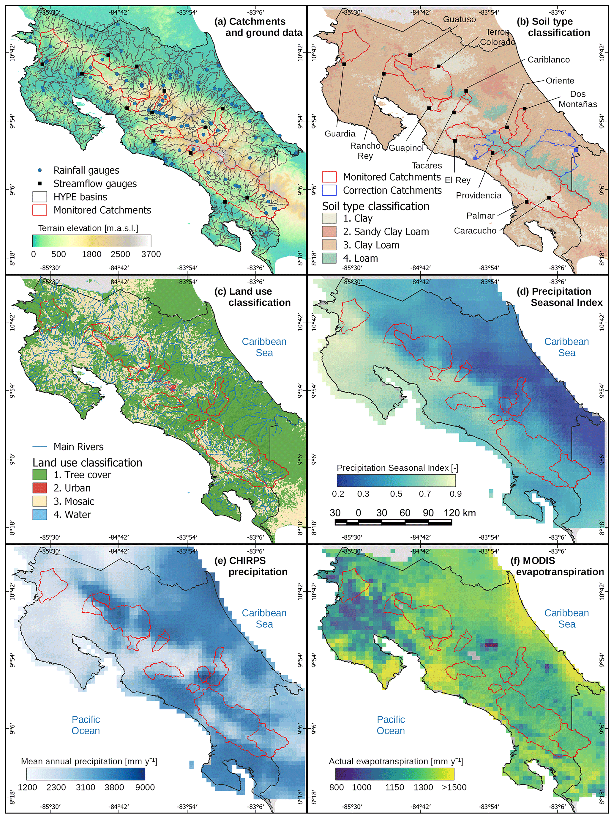
Figure 1 Study area (a) rainfall gauges (blue dots), monitored catchments (red polygons), and sub-basins used in the HYPE model (gray polygons), (b) soil type at 1 m depth from SoilGrids, where blue polygons correspond to catchments used for rain correction but not for calibration, (c) major land use categories from CCI Land Cover, (d) precipitation seasonal index with dark blue corresponding to uniform monthly precipitation and yellow to a more seasonal precipitation regime, (e) mean annual precipitation for the period 1981–2017 from CHIRPS, and (f) mean annual actual evapotranspiration for the period 2000–2014 from MODIS.

Table 1 Physical and climatological properties of the monitored catchments. Streamflow gauges were grouped according to their location in the Caribbean and the Pacific basins. AI stands for aridity index and EI stands for evaporative index.

Regarding model simulations, more than 600 nested catchments covering the whole country were delineated using the 30 m Shuttle Radar Topography Mission (SRTM) elevation model (Bamler, 1999) and the terrain analysis toolset from SAGA GIS v.6.4 (Conrad et al., 2015), where the fill sinks algorithm by Wang and Liu (2006) was applied with a minimum slope parameter of 0.0001^∘ and the flow accumulation top-down algorithm together with the single flow direction (D8) configuration. These parameters were defined following previous experience using SAGA with SRTM. Several issues were found during the delineation of catchments on flat terrain, where computed water courses differed from the actual river network. We corrected the computed river network using the vector layers of the main rivers from OpenStreetMap (OSM), forcing the water courses following Monteiro et al. (2018). The final catchments ranged from 3 to 500 km² with a median value of 65 km² and a main river length from 2.5 to 75 km with a median value of 15.2 km.

Figure 1b and c shows the soil types and land uses across Costa Rica, respectively. Soil types were derived from SoilGrids (Hengl et al., 2017; see dataset description in Table 2) and compared to national-scale soil maps. Sand content and clay content at 1 m depth were used to classify the soil types from the USDA classification criteria in SAGA GIS tools. Furthermore, in order to reduce the number of model parameters, only the four most frequent soil types were considered (Fig. 1b). The predominant soil texture is clay loam covering an area of ∼35 360 km² (69 % of Costa Rica), mainly across low elevation areas. Clay soils cover an area of ∼9740 km² (∼19 % of Costa Rica) and are located mainly along the Pacific Basin. Moreover, in high elevations loamy soils predominate, covering an area of ∼3800 km² (7 % of total area). The land use classes were obtained from the Climate Change Initiative Land Cover (CCI LC), where 19 unique land cover classes were found for Costa Rica. Similarly, the land use was reclassified into the four most common categories (Fig. 1c), where the predominant land uses were tree cover (∼65 %) and mosaic cover (∼34 %, which includes shrubs, grassland, sparse vegetation, croplands). Urban areas represent less than 0.5 % of Costa Rica. Different CCI LC tree categories were grouped into a single tree class, with ∼87 % corresponding to broadleaved evergreen trees. More than 98 % of the reclassified urban areas correspond to the original urban land use from CCI LC. The mosaic reclassification was mainly composed of mosaic natural vegetation and croplands (54 % and 13 %, respectively). Finally, the water reclassification consisted of 93 % water bodies and flooded shrub areas.

Table 2 Remote sensing and global products used in this study.

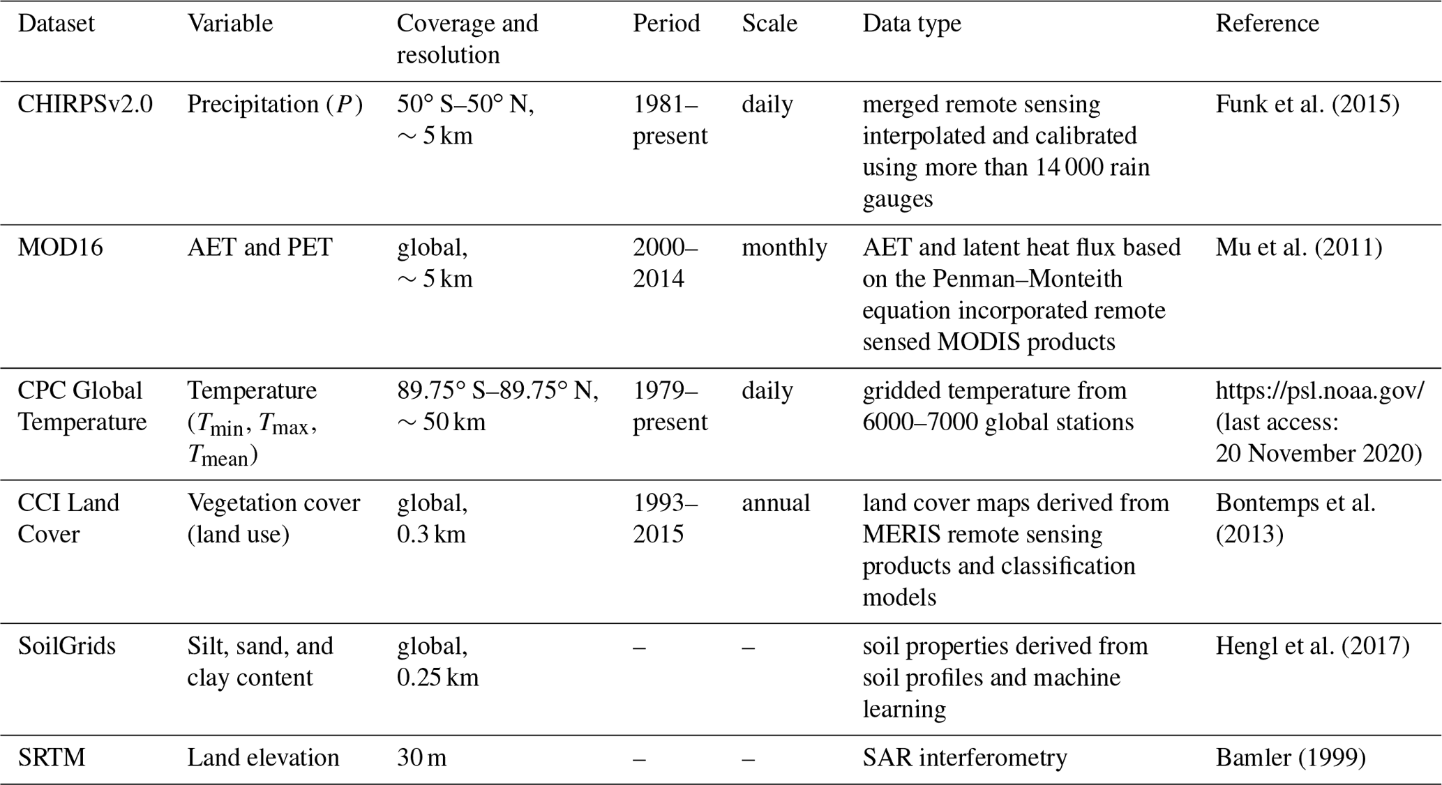
The climatological space–time series were obtained from remote sensing and global products, described in Table 2. The precipitation grid was obtained from the Climate Hazards Group InfraRed Precipitation with Satellite data (CHIRPS) version 2 (Funk et al., 2015), and the mean daily temperature was obtained from the CPC Global Daily Temperature product provided by the NOAA/OAR/ESRL PSL (https://psl.noaa.gov/, last access: 20 November 2020). Temperature exhibited low seasonality, with mean values ranging from 27 ^∘C in coastal regions to 20 ^∘C in the central region at around 1000 m a.s.l. (Esquivel-Hernández et al., 2017). Figure 1d shows the seasonality of monthly precipitation from CHIRPS using the index proposed by Walsh and Lawler (1981), where lower values (<0.3) correspond to a more uniform monthly precipitation, and higher values (>0.8) indicate that annual precipitation is concentrated over a few months. Such seasonality is widely controlled by air masses that reach Costa Rica at the Caribbean littoral, accumulating more humidity on the Caribbean slope (Sáenz and Durán-Quesada, 2015), shown as dark blue areas in Fig. 1d. Meanwhile, the humidity along the Pacific Basin is highly influenced by the migration of continental air masses of the Intertropical Convergence Zone (ITCZ), which establishes the rainy season in May–June and in September–November (Esquivel-Hernández et al., 2017; Muñoz et al., 2008).

The yearly cycle of wet and dry deviations in the ocean–atmosphere is linked to changes in the sea surface temperature of both the Pacific Ocean and the Caribbean Sea, where the El Niño Southern Oscillation (ENSO) is associated with a decrease of the mean annual precipitation across the Pacific Basin, and an increase of precipitation in the Caribbean Basin (Muñoz et al., 2008).

Moreover, the cold-phase La Niña is the cause of an increase in precipitation in the Pacific Basin and a decrease in the Caribbean (Waylen et al., 1996). Overall, the mean annual precipitation averaged ∼3000 mm for Costa Rica with maxima as high as 9000 mm, observed in the headwaters of the Reventazón catchment at the northwest of the Talamanca Mountain range and the Caribbean Basin (Fig. 1e). The minimum annual precipitation of 1200 mm yr⁻¹ is observed on the northern Pacific Basin in the Bebedero and Tempisque catchments.

The rainfall patterns across Costa Rica are reflected in the streamflow responses of catchments on the Pacific and Caribbean sides. The daily streamflow tends to be higher in the Caribbean Basin (9.2 mm d⁻¹ in comparison to 4.2 mm d⁻¹ on the Pacific side, computed from observed streamflow records, Table 1), mainly due to the seasonal climate across the Pacific slope with reduced water availability during the dry season from December to April. Furthermore, the stream lengths of rivers on the Caribbean slope tend to be longer in comparison with rivers from the Pacific Basin (see the river network in Fig. 1c).

Potential evapotranspiration and actual evapotranspiration were obtained from the MODIS product (Mu et al., 2011) distributed by the Numerical Terradynamic Simulation Group at the University of Montana, USA, which compared well to the few available ground stations in Costa Rica, with errors from −0.3 to 0.7 mm yr⁻¹ (Esquivel-Hernández et al., 2017). Even though several products of AET and PET are available at higher temporal resolution (such as GLEAM at a daily time step; Miralles et al., 2011), the spatial resolution of these products is at least 5 times lower than MODIS ($\sim \mathrm{5}\times \mathrm{5}$ km, ∼25 km²). Since ∼70 % of our delimited catchments are smaller than 100 km², the spatial resolution of the global products plays an important role in capturing the spatial variability of the water balance for modeling.

Figure 1f shows the mean annual AET from MODIS, which spatially ranges from 547 to 1612 mm. The highest AET values were observed at the coast (Caribbean and Pacific). Moreover, the lower AET values overlap with low humidity zones and sparse vegetation areas (northwestern Costa Rica), as well as higher elevation cloud cover that decreases soil evaporation (Caribbean slope mountain region).

3 Materials and methods

3.1 HYPE model structure and setup

We used Hydrological Predictions for the Environment (HYPE) version 5.9, a semi-distributed hydrological model, for the assessment of water resources and water quality at small and large scales (Lindström et al., 2010) in order to simulate the hydrological response of Costa Rican catchments. The HYPE model can be considered as the evolution of the distributed Hydrologiska Byråns Vattenbalansavdelning (HBV) model (Lindström et al., 1997). HYPE was developed by the Swedish Meteorological and Hydrological Institute (SMHI) as the operative model for drought and flood forecasting across Sweden (Pechlivanidis et al., 2014). Moreover, HYPE was recently applied to other climatic regions (Andersson et al., 2017; Arheimer et al., 2018; Berg et al., 2018; Lindström, 2016; Pugliese et al., 2018; Tanouchi et al., 2019), including a global-scale application (Arheimer et al., 2020).

The HYPE model allows simulating the water balance and nutrient fluxes at a daily or sub-daily scale using precipitation and temperature as forcings (SMHI, 2018). The model structure (Fig. 2a) describes the major water pathways and fluxes, ensuring mass conservation at the catchment and sub-catchment scale. Furthermore, each sub-catchment is divided into the most fundamental spatial soil and land use classes (SLCs) depending on the classification of soil types, land cover, climate, and elevation, as shown in Fig. 2b. The SLCs in HYPE provide the capability to predict streamflows in ungauged basins since the parameters that regulate the fluxes and storages are linked to each SLC, with a maximum of three layers of different soil thickness, as shown in Fig. 2b. Water bodies such as lakes and rivers may be considered as an SLC, where lakes can be defined as natural lakes or regulated dams with multiple water outputs. For full details of the HYPE model, see the description by Lindström et al. (2010) and the open-access code references located at https://hypeweb.smhi.se/model-water/ (last access: 10 June 2021).

Figure 2 Schematic representation of the HYPE model (a) division into sub-basins and local classes according to topography, land use, and soil classes and (b) the model structure of Basin 1 considering two main soil–land combinations and lake properties. In (b), the simulated hydrological processes and variables are shown in black, while parameter names are given in blue. A full description of parameters (in blue) is available at https://hypeweb.smhi.se/model-water/ (last access: 10 June 2021). The ilake parameter corresponds to an internal lake and the olake parameter to an outlet lake. T is temperature, P is precipitation, ET is evapotranspiration, Q_t is streamflow, and GW is groundwater.

For this study, Costa Rica was divided into 605 catchments (Fig. 1a) with 12 SLCs obtained from the spatial combination of soil types and land cover maps shown in Fig. 1b and c, respectively. Outlet lakes (which discharge to downstream catchments) and internal lakes (which discharge into the main river or tributaries) were set up as different SLCs to consider the water bodies that regulate the streamflow. The largest water body in Costa Rica is the Arenal reservoir, located in the San Carlos River catchment (Fig. 1b). The Arenal reservoir is an artificial lake used for hydropower purposes with an average surface area of 87.8 km² and a depth that ranges from 30 to 60 m. The Arenal reservoir was implemented as a natural lake since its operational rules are confidential and therefore unknown.

Soil thickness varied for different SLCs, with a maximum soil thickness of 3 m under forests and a minimum of 2 m for bare soil cover, following Arheimer et al. (2020). Furthermore, delimited catchments were classified according to their elevation and location (Pacific Basin and Caribbean Basin), applying regional factors to correct the hydrological behavior of lowland and mountainous catchments with similar SLCs, resulting in six defined regions.

Daily time series of precipitation from CHIRPS and temperature from NOAA for the period 2000–2014 were extracted for each catchment using GRASS GIS (Neteler et al., 2012), where datasets were resampled to 1 km using the nearest-neighbor criteria and spatially averaged for each catchment. The climatological forcings were resampled due to the small size of some catchments (area of ∼1 km²). Arheimer et al. (2020) recommended computing the average of the nearest grids to obtain the forcings instead of deriving the data from the nearest pixel.

3.2 Precipitation correction

Rainfall estimations from satellites are subject to systematic errors that may produce uncertainty in hydrological simulations (Goshime et al., 2019; Grillakis et al., 2018; Infante-Corona et al., 2014; Wörner et al., 2019). The CHIRPS product already incorporates a bias correction procedure but uses only a few concentrated ground stations in Costa Rica. The performance of CHIRPS estimating annual water balances is shown in Fig. S1a and c in the Supplement, with frequent underestimation in the monitored catchments. Therefore, we applied a linear scaling to further correct for the bias between the product and ground precipitation from 75 available stations across Costa Rica (Fig. 1a). The corrected precipitation was estimated as

$$\begin{array}{}\text{(1)}& {\mathrm{CHIRPS}}_{\mathrm{c}}\left(t\right)=\mathrm{CHIRPS}\left(t\right)\cdot \mathrm{BF},\end{array}$$

where CHIRPS_c is the bias-corrected precipitation at time t, CHIRPS is the original precipitation at time t, and BF is the bias factor. The bias factor was estimated as

$$\begin{array}{}\text{(2)}& \mathrm{BF}={\displaystyle \frac{\mathit{\mu }\left(P\right)}{\mathit{\mu }\left(\mathrm{CHIRPS}\right)}},\end{array}$$

where μ(P) is the mean of the historical precipitation from the ground stations, and μ(CHIRPS) is the mean of the historical precipitation from CHIRPS. Note that μ(P) and μ(CHIRPS) were computed using the common study period. The simple linear bias correction was preferred over more complex methods due to the lack of a long common period for all stations. Therefore, we used the individual records of more than 60 available stations covering a period from 1980 to 2010 to better capture the complex topography and resulting rainfall patterns.

Some monitored catchments exhibiting higher annual streamflow than annual precipitation could not be corrected due to groundwater contributions from neighboring catchments (Genereux and Jordan, 2006; Genereux et al., 2002), under-catch at rainfall gauges (Frumau et al., 2011), and the insufficient number of precipitation stations to correct the CHIRPS database at a national scale. Nevertheless, errors in climatological data have been found to be the most common issue for water balance modeling in Central America (Westerberg et al., 2014; Birkel et al., 2012). In that sense, an additional approach was implemented to reduce the unrealistic relationship between streamflow and precipitation, which consisted of the creation of virtual stations at the catchment centroid, where the new bias factor was computed as

$$\begin{array}{}\text{(3)}& {\mathrm{BF}}_{\mathrm{2}}={\displaystyle \frac{\mathit{\mu }\left(Q_{t_{\mathrm{y}}}\right)+\mathit{\mu }\left({\mathrm{AET}}_{\mathrm{y}}\right)}{\mathit{\mu }\left({\mathrm{CHIRPS}}_{\mathrm{y}}\right)}},\end{array}$$

where μ refers to the mean value, $Q_{t_{\mathrm{y}}}$ is the annual streamflow from 1990 to 2003, AET_y is the MODIS annual actual evapotranspiration from 2001 to 2014, and CHIRPS_y is the CHIRPS annual precipitation from 1990 to 2014. BF₂ adjusts the long-term precipitation volume to ensure that the water balance is preserved, avoiding underestimation of streamflow and evapotranspiration. Four streamflow gauges in addition to those shown in Table 1 were used to cover additional spatial area at high elevations for the correction of satellite-based precipitation. These streamflow gauges were omitted from the model calibration–validation procedure due to their shorter records (less than 7 years). The location of the four streamflow gauges and their catchments are shown in Fig. 1b.

Finally, BF points from precipitation stations and BF₂ from virtual points were interpolated using the inverse distance weighted (IDW) method (Shepard, 1968), with an exponent value of 2 at the original CHIRPS resolution. The interpolated map of the bias factor was used to spatially correct the time series of CHIRPS across Costa Rica.

3.3 Evapotranspiration and temperature correction

HYPE incorporates four methods for PET estimation (SMHI, 2018). After initial tests, we found that the monthly PET signal from MODIS in Costa Rica can be reproduced by only using temperature as forcing, where PET is computed as

$$\begin{array}{}\text{(4)}& \mathrm{PET}=\left(\mathrm{cevp}\cdot \mathrm{cseason}\right)\cdot \left(\mathrm{temp}-\mathrm{ttmp}\right)\cdot \left(\mathrm{1}+\mathrm{cevpcorr}\right),\end{array}$$

where PET is the daily potential evapotranspiration (in millimeters), temp is the daily mean air temperature (^∘C), cevp is an evapotranspiration parameter that depends on the land use (mm ^∘C⁻¹ d⁻¹), ttmp is a threshold temperature for evapotranspiration (^∘C), cevpcorr is a correction factor for evapotranspiration, and cseason is a factor computed as

$$\begin{array}{}\text{(5)}& \mathrm{cseason}=\mathrm{1}+\mathrm{cevpam}\cdot \sin \left({\displaystyle \frac{\mathrm{2}\cdot \mathit{\pi }\cdot \left(\mathrm{dayno}-\mathrm{cevpph}\right)}{\mathrm{365}}}\right),\end{array}$$

where cevpam is a correction factor, dayno is the day of the year, and cevpph is a factor used to correct the phase of the sine function in order to correct the potential evapotranspiration (set as zero in this study). To deal with the coarse spatial resolution of the temperature database (0.5^∘), a correction factor that depends on catchment elevation was computed (SMHI, 2018):

$$\begin{array}{}\text{(6)}& \mathrm{tempc}=\mathrm{temp}-{\displaystyle \frac{\mathrm{tcelevadd}\cdot \mathrm{elev}}{\mathrm{100}}},\end{array}$$

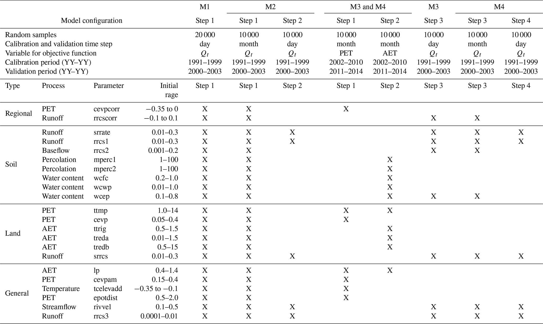
where tempc is the corrected air temperature (in ^∘C), temp is the original air temperature (^∘C), tcelevadd is a calibrated parameter that corrects temperature (^∘C 100⁻¹ m⁻¹), and elev is the mean catchment elevation (m). Since only few (<10) temperature station records were available, a bias correction procedure was not possible, but measured temperature closely followed the environmental lapse rate (Esquivel-Hernandez et al., 2017). The parameters cevp, cevcorr, cevpam, and tcelevadd are part of the Monte Carlo simulation and their ranges are shown in Table 3.

Table 3 Parameter names and initial ranges of the step-wise parameter estimation for each model configuration. Columns M1, M2, M3, and M4 correspond to parameters optimized during each step of the configuration, and Q_t, PET, and AET correspond to the observed time series used to calibrate the model configurations. $Q_{t_{\mathrm{d}}}$ means daily streamflow, $Q_{t_{\mathrm{m}}}$ monthly streamflow, PET_m monthly potential evapotranspiration, and AET^m monthly actual evapotranspiration.

3.4 Model calibration procedure

Figure 3 shows the workflow adopted for model calibration, which involves a qualitative parameter sensitivity analysis to find the most suitable range of values for the automatic calibration. The initial parameter ranges were obtained from manual iterations of one parameter at a time to facilitate automatic calibration (Infante-Corona et al., 2014).

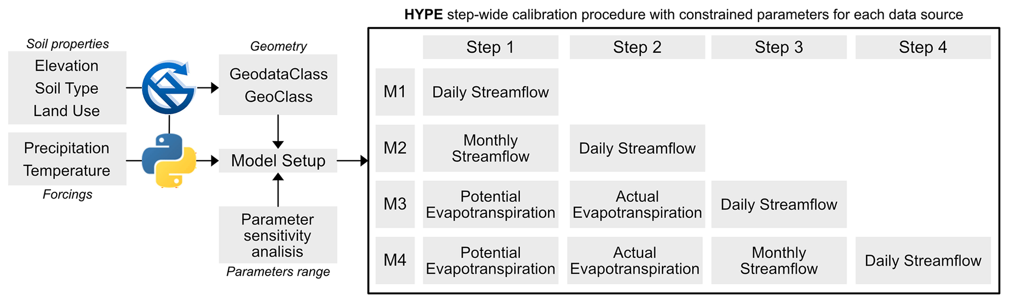
Figure 3 Schematic representation of the HYPE model calibration strategy considering a step-wise procedure to constrain parameters. Four model configurations (M1, M2, M3, M4) were established using different data sets and/or different timescales. From each calibration step, the 10th and 90th values of the best-fit parameters were used to constrain the parameters of the next step.

We considered four model configurations to analyze the effect of including PET and AET in model calibration:

• model configuration 1 (M1), calibrated using only daily streamflow (Q_t);

• model configuration 2 (M2), calibrated using monthly streamflow followed by daily streamflow;

• model configuration 3 (M3), incorporating a calibration using monthly PET and AET, followed by daily streamflow;

• model configuration 4 (M4), similar to M3, additionally using monthly streamflow before daily streamflow calibration.

For comparison purposes, M1 was chosen as the baseline model configuration, which usually is standard in hydrological practice. The steps are described in Fig. 3. The common period between Q_t and PET-AET is relatively short (3 years), resulting in Q_t and PET-AET calibration using different steps. The automatic calibration consisted of a step-wise procedure, where each model configuration was calibrated for different fluxes (daily Q_t, monthly Q_t, monthly AET, monthly PET). The parameter names and initial ranges used for the calibration steps and their configuration are shown in Table 3 and Fig. 2. A final step (not shown in Fig. 3) consisted of calibrating the curve discharge parameters of the Arenal reservoir using observed water levels. However, the Arenal infrastructure does not contribute to the downstream basins and has a poor impact on the regional model calibration. Moreover, as previously stated, the reservoir was simulated as a lake since its operational rules are unknown.

The streamflow records were divided into the period from 1991 to 1999 for calibration and from 2000 to 2003 for validation. The PET and AET calibration period was established as 2002 to 2010 and the validation period as 2011 to 2014. In both cases, for model warm-up we ran it for 2 years prior to calibration since our modeling tests showed that using 2 years was enough to stabilize the effects of initial conditions of water content in soil layers, rivers, and reservoirs. The 13 monitored catchments were used for streamflow calibration. For PET and AET calibration steps, only the 130 catchments within the 13 monitored catchments were used since our tests showed that using the 605 catchments did not significantly increase the model performance but it did increase the calibration time by a factor of 5. The simulations of the 605 catchments were used to compute the metrics for the calibration and validations periods.

A total of 86 parameters were used to build the HYPE model structure consisting of 36 parameters linked to four soil types, 24 parameters linked to four land cover classes, 6 parameters for the general structure, 12 parameters for the regional correction of PET and temperature, and 8 parameters for lake discharge. The Monte Carlo (MC) routine for parameter sampling and sensitivity analysis included in HYPE was used for calibration, and the model configurations were run 10 000 times for each step, except for M1, which used 20 000 runs to cover more parameter combinations since this configuration only used daily streamflow. Despite the lower computational efficiency of the MC with respect to other optimization schemes (such as gradient-based methods), the MC routines are more flexible in accounting for multiple parameters sets in complex models (Beven, 2006). The 10th and 90th percentiles of the resulting parameters from the best 100 runs were used to constrain the parameters for the next calibration step.

3.5 Model calibration and validation using hydrological signatures

The CHIRPS product was evaluated with ground records using the false alarm rate (FAR, computed with Eq. 7), probability of detection (PD, computed with Eq. 8), and threat score (TS, computed with Eq. 9):

$$\begin{array}{}\text{(7)}& {\displaystyle }& {\displaystyle }\mathrm{FAR}={\displaystyle \frac{\mathrm{false}\mathrm{alarms}}{\mathrm{hits}+\mathrm{false}\mathrm{alarms}}},\text{(8)}& {\displaystyle }& {\displaystyle }\mathrm{PD}={\displaystyle \frac{\mathrm{hits}}{\mathrm{hits}+\mathrm{misses}}},\text{(9)}& {\displaystyle }& {\displaystyle }\mathrm{TS}={\displaystyle \frac{\mathrm{hits}}{\mathrm{hits}+\mathrm{false}\mathrm{alarms}+\mathrm{misses}}},\end{array}$$

where hits are days with precipitation detected by CHIRPS and ground rain gauges, false alarms are days where precipitation was detected only by CHIRPS, and misses are days where precipitation was detected only by rain gauges.

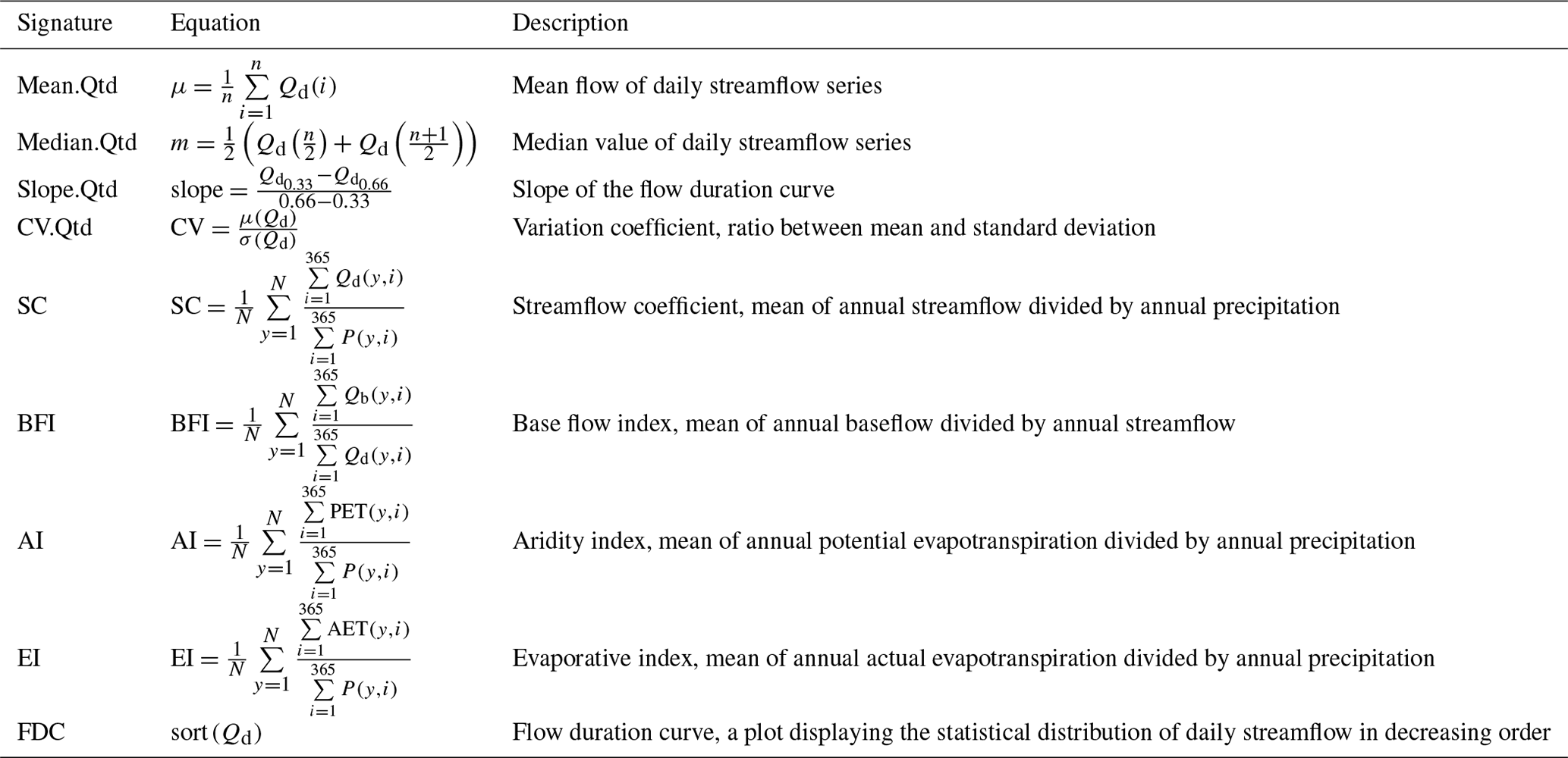
Table 4 Hydrological signatures used as independent performance evaluation criteria.

The model performance was evaluated using the Kling–Gupta efficiency (KGE; Kling and Gupta, 2009), computed as

$$\begin{array}{}\text{(10)}& {\displaystyle }& {\displaystyle }\mathrm{KGE}=\mathrm{1}-\sqrt{(r-\mathrm{1}{)}^{\mathrm{2}}+(\propto -\mathrm{1}{)}^{\mathrm{2}}+(\mathit{\beta }-\mathrm{1}{)}^{\mathrm{2}}},\text{(11)}& {\displaystyle }& {\displaystyle }r=\mathrm{CC}={\displaystyle \frac{\mathrm{cov}\left(x_{\mathrm{o}},x_{\mathrm{s}}\right)}{{\mathit{\sigma }}_{\mathrm{o}}{\mathit{\sigma }}_{\mathrm{s}}}},\text{(12)}& {\displaystyle }& {\displaystyle }\propto ={\displaystyle \frac{{\mathit{\sigma }}_{\mathrm{s}}}{{\mathit{\sigma }}_{\mathrm{o}}}},\text{(13)}& {\displaystyle }& {\displaystyle }\mathit{\beta }={\displaystyle \frac{{\mathit{\mu }}_{\mathrm{s}}}{{\mathit{\mu }}_{\mathrm{o}}}},\end{array}$$

where subscripts “o” and “s” correspond to observations and simulations, respectively. μ is the mean, x is the time series (streamflow, actual evapotranspiration, or potential evapotranspiration), σ is the standard deviation, r and CC are the correlation coefficient, α is the agreement between amplitudes, and β is the bias. KGE was chosen as the objective function for calibration since it equally captures maximum and minimum flows (e.g., Arheimer et al., 2020; Pechlivanidis and Arheimer, 2015; Rajib et al., 2018a; Rakovec et al., 2016; Xiong and Zeng, 2019), and has been described as a relatively balanced metric with slightly more focus on high flows (Garcia et al., 2017). Non-transformed data were used given the advice of Santos et al. (2018) against using log-transformed discharge with the KGE for low flow evaluation. Furthermore, other statistical criteria were computed to facilitate assessing the performance of the model configurations, such as the Pearson correlation coefficient (computed with Eq. 11), mean absolute error (MAE, computed with Eq. 14), Nash–Sutcliffe efficiency (NSE, computed with Eq. 15), root mean square logarithmic error (RMSLE, computed with Eq. 16), and relative bias (Eq. 17):

$$\begin{array}{}\text{(14)}& {\displaystyle }& {\displaystyle }\mathrm{MAE}={\displaystyle \frac{\mathrm{1}}{n}}\sum _{i=\mathrm{1}}^n\left|x_{\mathrm{s}}\left(i\right)-x_{\mathrm{o}}\left(i\right)\right|,\text{(15)}& {\displaystyle }& {\displaystyle }\mathrm{NSE}=\mathrm{1}-{\displaystyle \frac{\sum _{i=\mathrm{1}}^n{\left(x_{\mathrm{s}}\left(i\right)-x_{\mathrm{o}}\left(i\right)\right)}^{\mathrm{2}}}{\sum _{i=\mathrm{1}}^n{\left(x_{\mathrm{o}}\left(i\right)-{\mathit{\mu }}_{\mathrm{o}}\right)}^{\mathrm{2}}}},\text{(16)}& {\displaystyle }& {\displaystyle }\mathrm{RMSLE}=\sqrt{{\displaystyle \frac{\sum _{i=\mathrm{1}}^n{\left(\log \left(x_{\mathrm{s}}\left(i\right)\right)-\log \left(x_{\mathrm{o}}\left(i\right)\right)\right)}^{\mathrm{2}}}{n}}},\text{(17)}& {\displaystyle }& {\displaystyle }\mathrm{Bias}={\displaystyle \frac{{\mathit{\mu }}_{\mathrm{s}}-{\mathit{\mu }}_{\mathrm{o}}}{{\mathit{\mu }}_{\mathrm{o}}}}.\end{array}$$

Furthermore, hydrological signatures were calculated to independently assess how well the calibrated model configurations reproduced different hydrological criteria. The hydrological signatures used in this study are shown in Table 4 and the Budyko curve was constructed from the aridity index (AI) and evaporative index (EI).

Finally, the non-parametric Kruskal–Wallis (Kruskal and Wallis, 1952) and Mann–Whitney (Mann and Whitney, 1947) tests were used to detect statistically different performance.

4 Results

4.1 Remote sensing input data bias correction and evaluation

Comparing precipitation from CHIRPS with annual streamflow and streamflow plus evapotranspiration (assuming long-term balance $P-Q_t-\mathrm{AET}=\mathrm{0}$) showed an underestimation of annual precipitation (as shown in Fig. S1a and c), leading to unrealistic water balance values. The interpolated bias correction factor (BF, Fig. 4a) showed an overestimation of CHIRPS rainfall in blue and underestimations in red. The BF ranged from 0.65 to 1.57 with an average of 1.06±0.14, where the greater disagreements between the ground precipitation and satellite-merged precipitation were observed along the Pacific Basin. The underestimation reached 30 % to 35 % in the north of the Gulf of Nicoya and in the southwest of the Providencia catchment. Underestimation of CHIRPS across the Caribbean slope was mainly observed in the Terron Colorado and Cariblanco catchments, with a BF between 1.2 and 1.4. Moreover, the largest overestimation of CHIRPS was observed for the Guanacaste region (BF = 0.65–0.8), downstream of the Tacares catchment (BF = ∼0.8), and to the southeast of Costa Rica (BF = 0.8–0.85).

Figure 4 Performance of the CHIRPS precipitation product in representing observed rainfall in Costa Rica. (a) Interpolated bias factor, where red areas indicate underestimation and dark blue areas overestimation of CHIRPS with respect to ground stations, and (b) cross correlations between daily precipitation from CHIRPS and observed daily streamflow, where high correlation values without delay (at zero) indicate that precipitation and high flows tend to occur on the same day. A high correlation with negative delays indicates that precipitation occurred on average before the streamflow response.

For modeling purposes, we evaluated the temporal synchronicity of rainfall versus streamflow (Fig. 4b) using cross-correlation between daily streamflow and catchment-scale daily precipitation from CHIRPS, where the x axis corresponds to the lag time in days. Most of the monitored catchments exhibited the highest correlation within lag time zero, indicating that the hydrological response of catchments tends to occur within the same day. Nevertheless, the Cariblanco and Rancho Rey catchments exhibited poor correlation (ρ<0.3), which means a lack of synchrony between daily satellite-merged precipitation and streamflow.

The bias correction improved the annual precipitation where CHIRPSc was consistent with annual streamflow, and the long-term water balance was mostly preserved, as observed in Fig. S1b and d. Figure S2 shows the MAE normalized by mean precipitation for CHIRPS and bias-corrected CHIRPS (CHIRPSc), both with respect to the 75 precipitation stations, where boxplots correspond to the variability of normalized MAE estimated by each point. The average normalized MAE at a daily scale was estimated at 1.2±0.12 mm mm⁻¹ for CHIRPS and 1.17±0.08 mm mm⁻¹ for CHIRPSc, 0.30±0.09 and 0.27±0.07 mm mm⁻¹ at a monthly scale, and 0.16±0.09 and 0.11±0.04 mm mm⁻¹ at an annual scale, respectively.

Figure S2d shows the probability of success and failure of CHIRPSc at detecting rainy or dry days with respect to ground stations, where the probability was computed from a single time series merged from the 75 station records. Furthermore, Fig. S2e to g show the false alarm rate (FAR), probability of detection (PD), and threat score (TS), respectively. Results indicated that CHIRPSc detected true rainy and dry days with a similar probability (0.31 to 0.34) as in situ observed rainfall, whereas the FAR ranged from 0.15 to 0.38 with the greater values (i.e., incorrect detection of dry days as rainy days by CHIRPS) to the southeast, and the PD showed greater values (i.e., better performance of CHIRPS at detecting rainy days) for the Pacific Basin (median of ∼0.69) in comparison with the rain gauges in the Caribbean Basin (median PD of ∼0.54). The TS showed similar results to PD (Fig. S2g), with better performance of CHIRPS for the Pacific Basin (median of ∼0.53) than for the Caribbean Basin (median of ∼0.46). Such low capacity of CHIRPS to detect rainy days in the Caribbean Basin could affect the performance of the hydrological model during peak flows.

4.2 Model performance and parameter uncertainty

Figure 5 shows the comparison of the model configurations' performance for the calibration (dark blue) and validation (light blue) periods. Simulated daily streamflow for the 13 gauged catchments was similar for baseline configuration (M1) and M2 during the calibration period (1991–1999; Fig. 5a) with a mean KGE of 0.54±0.09 and 0.53±0.08, respectively. Nevertheless, M1 showed a median NSE of 0.33 in comparison to M2, which showed a median NSE of 0.25. The comparison of the correlation coefficient, median absolute error, and NSE metrics is shown in Fig. S3. Moreover, metrics for M3 and M4 were slightly poorer due to a larger dispersion across the sample, with a mean KGE of 0.45±0.2 and 0.47±0.17, respectively, and a mean NSE of 0.23±0.2 and 0.21±0.21. For the validation period (2000–2003), the mean KGE decreased by ∼0.08, but with similar performance for NSE.

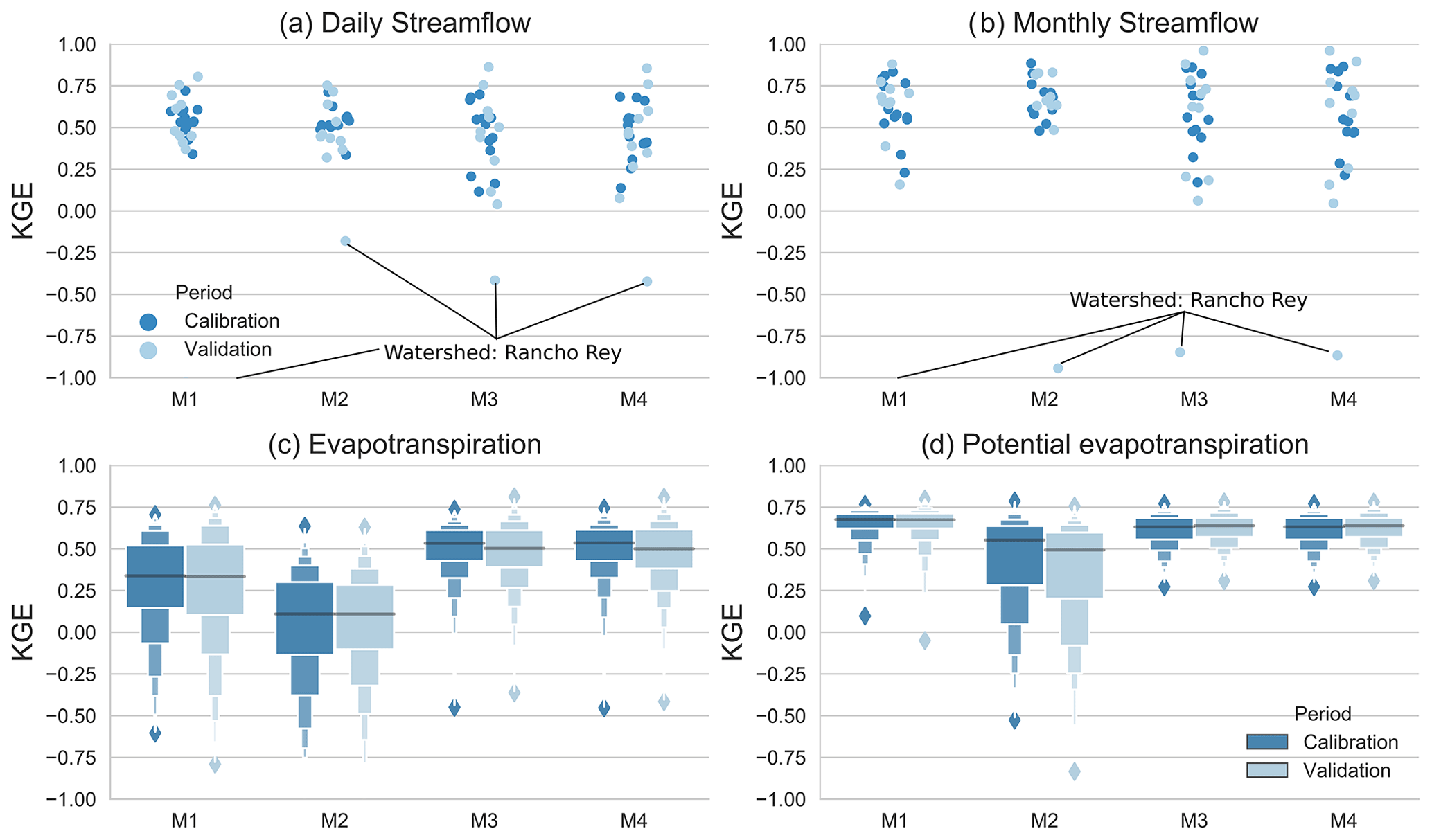
Figure 5 The range of KGE values for the calibration (dark blue) and validation periods (light blue). (a) KGE statistical dispersion for daily streamflow, (b) KGE statistical dispersion for monthly streamflow, (c) boxplots of KGE values for AET, and (d) boxplots of KGE for PET. Streamflow calibration period from 1991 to 1999 and validation period from 2000 to 2003. PET and AET calibration period from 2001 to 2010 and validation period from 2011 to 2014. Since the configurations M1 and M2 were calibrated only with streamflow, panels (c) and (d) are for comparison purposes only, showing the effect of including PET and AET in the calibration procedure.

The configuration M2 best reproduced monthly streamflow for the calibration period (Fig. 5b), with a mean KGE of 0.67±0.11, whereas the configurations M1, M3, and M4 showed a mean KGE of ∼0.60, also driven by larger dispersion along the KGE scale. The NSE also supports M2 as the best monthly streamflow predictor for the calibration period (Fig. S3), with a median value of 0.54, in contrast to M1, which showed a median NSE of 0.43. The four model configurations preserved performance for the validation period, and in some cases, the KGE even increased, as was the case for the Palmar, Caracucho, and El Rey catchments (not shown). Nevertheless, the Rancho Rey catchment exhibited poor performance during the validation period (KGE < 0 and NSE < −2) for daily and monthly scales since the four configurations overestimated streamflow. In the following sections, we present more details for Rancho Rey that can explain the catchment behavior and its performance.

Figure 5c and d show the effect of including AET and PET in the calibration steps, and the KGE was computed by aggregating the complete domain (605 nested catchments). The calibration consisted of 130 nested catchments within the monitored catchments. Furthermore, M1 and M2 were only plotted for comparison purposes since these configurations were calibrated with streamflow. From Fig. 5c, we observed that simulated monthly AET for the calibration period (2002–2010) improved for M3 and M4 with a mean KGE of $\sim \mathrm{0.49}\pm \mathrm{0.17}$ with respect to M1 with a mean KGE of 0.29±0.29 and M2 (0.04±0.33). The higher performance of AET was also observed for M3 and M4 according to the correlation coefficient and MAE (Fig. S3). Surprisingly, the baseline configuration (M1) showed a slightly better performance of simulated monthly PET, with a mean KGE of 0.64±0.09, whereas M3 and M4 showed a mean KGE of $\sim \mathrm{0.61}\pm \mathrm{0.10}$, and M2 a mean KGE of 0.43±0.28 (Fig. 5d). The performance of monthly AET and monthly PET was similar for the validation period (2011–2014; Fig. S3).

The results from Fig. 6 suggested that the best performance of daily and monthly streamflow for the calibration period (2001–2009) was obtained for catchments in the southeast of Costa Rice, such as the Palmar, Caracucho, El Rey, and Guapinol catchments, with KGEs higher than 0.55 (NSE > 0.4, as shown in Fig. S4) for daily streamflow and higher than 0.8 (NSE > 0.63) for monthly streamflow. Nevertheless, the mid-Pacific Basin also resulted in the Tacares and Providencia catchments exhibiting the worst performance for monthly streamflow and the configurations M3 and M4 with KGE < 0.3 and NSE < 0 (Fig. 6g and h).

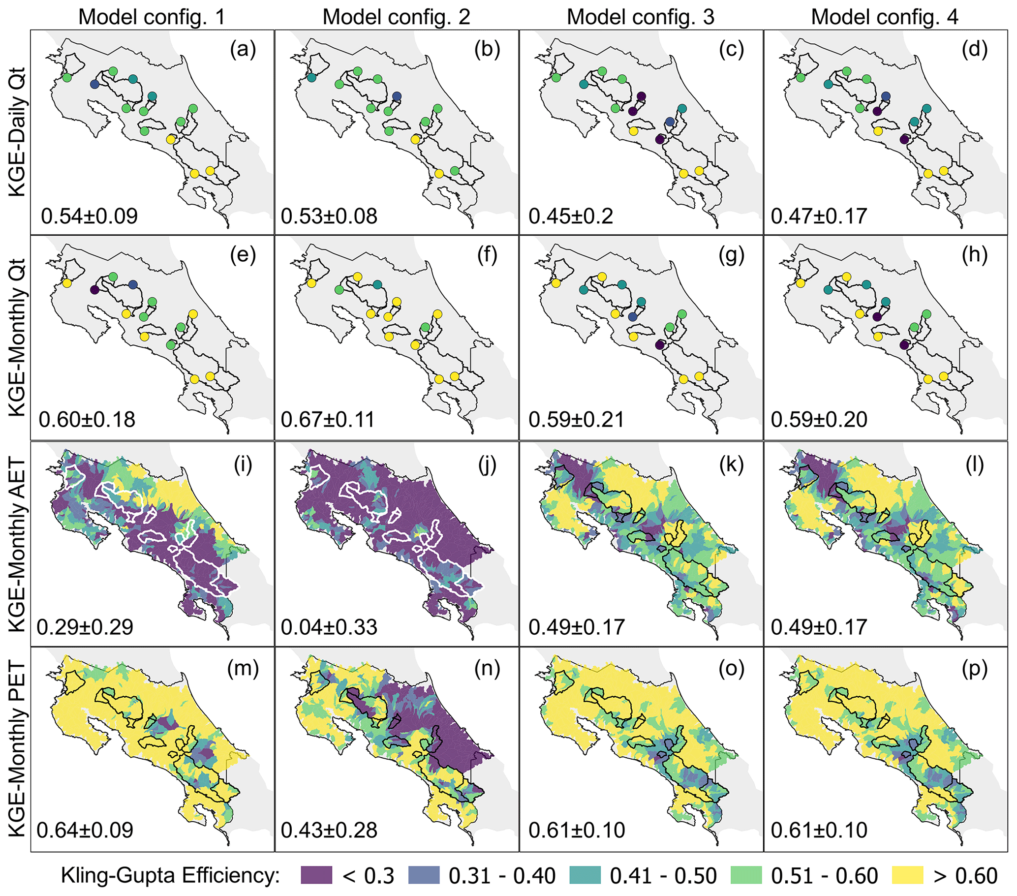
Figure 6 Matrix of spatially distributed KGE results for the calibration period (streamflow from 1991 to 1999, PET and AET from 2001 to 2010), where green and blue reflect better performance. Configurations M1 and M2 were calibrated only with streamflow. Nevertheless, PET and AET panels are compared to show the effect of including such variables in the calibration procedure. The mean ± SD of KGE is shown on the lower left of each panel.

The spatially distributed KGE on the last two panels of Fig. 6 shows the improvement by including AET and PET in the calibration steps (Fig. 6k, l, o and p), unlike the case of daily and monthly Q_t, where no significant improvements were observed using the four calibration procedures. The calibrated monthly AET simulated with M1 showed low efficiency (KGE < 0.2 and NSE < 0) for ∼182 catchments of the Pacific Basin but an acceptable performance (KGE > 0.6 and NSE > 0.2) for monthly PET. M2 exhibited poor performance across the simulation domain for AET and low efficiency of PET in the southeast Caribbean. Additionally, M3 and M4 showed similar results with acceptable performance (KGE > 0.6 and NSE > 0.2) for ∼179 catchments, most of them located in the northeast. The median MAE and the median correlation coefficient for M3 and M4 were ∼11 % lower (MAE = ∼15 mm) and ∼39 % higher (CC > 0.63) than for M1. Surprisingly, the simulated PET with M3 and M4 was similar to the PET from M1. The performance of the calibrated water level on the Arenal reservoir was relatively low for all configurations (KGE ∼ 0.35, NSE < −0.1, and CC ∼ 0.36), affected by the unknown quantity of withdrawals from the reservoir during the driest months (April–July).

Figure 7 shows the model parameter ranges from the 100 best-fit simulations resulting from the last calibration step for each configuration. The red dots from Fig. 7 correspond to the optimal parameters used for modeling, where multiple red dots and boxplots for each model are shown by soil type and land use.

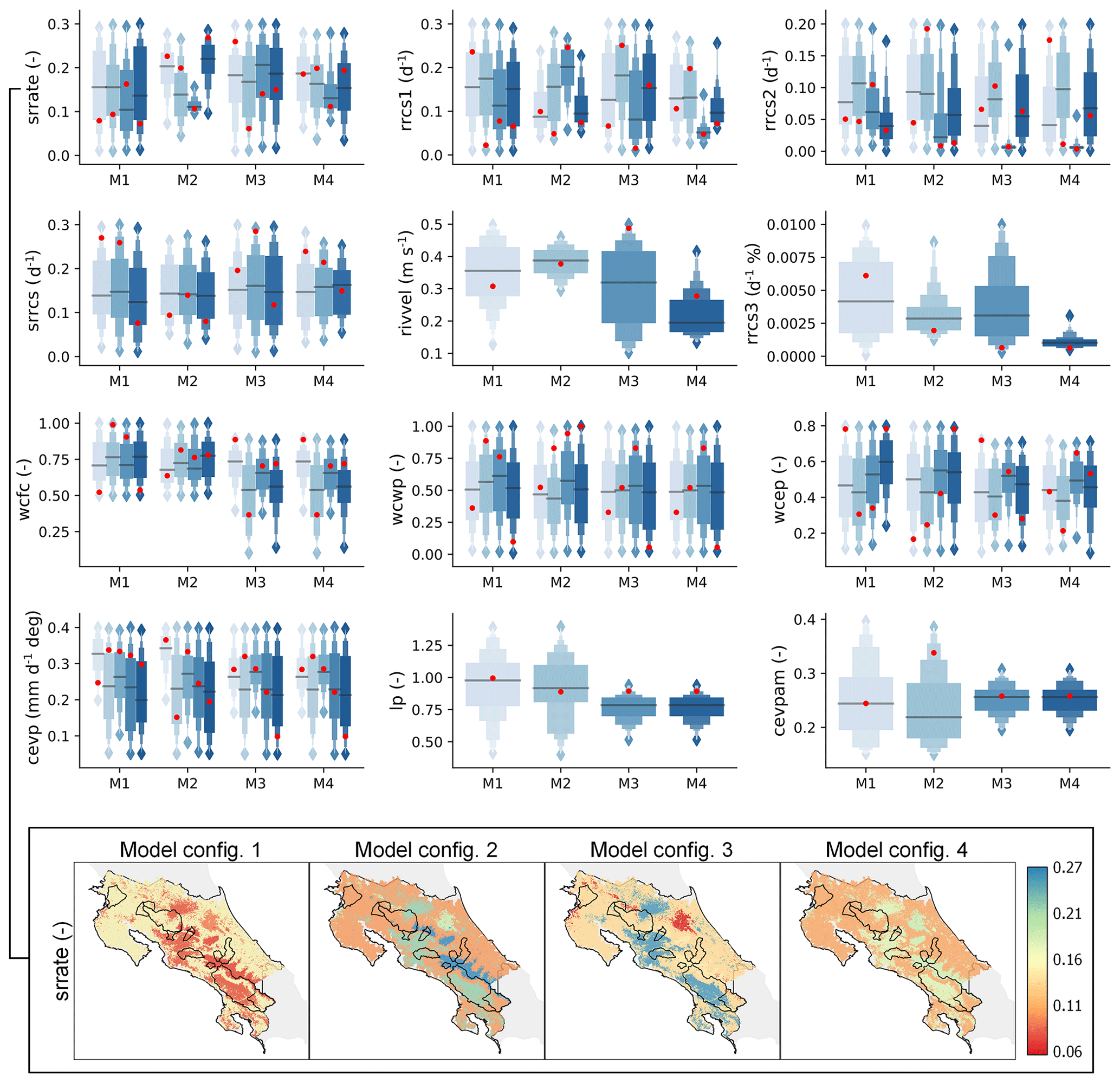
Figure 7 A posteriori parameter distribution for the 100 best-fit simulations from the last calibration step for each configuration, where red dots correspond to the optimal parameters. Multiple boxplots for each model configuration correspond to the parameters of different soil and land classes. The top two rows of parameter panels correspond to streamflow components, the third row to water content parameters, and the fourth row to PET and AET processes (see Table 3 for reference). For comparison purposes, the bottom row shows the spatial variability of the best-fit calibrated srrate (–) parameter for each configuration.

A large dispersion with a coefficient of variation (CV = SD/mean) greater than 0.35 was observed for runoff response parameters (srrate, fraction for surface runoff; srrcs, recession coefficient for surface runoff) and baseflow parameters (rrcs1, recession coefficient for uppermost soil layer; rrcs2, recession coefficient for lowest soil layer). The impacts of monthly streamflow on calibration were observed for the general model parameters of rivvel (river velocity) and rrcs3 (deep layer recession coefficient), with constrained posterior parameter distributions for configurations M2 and M4 and higher velocities and greater baseflow discharge for M2 with respect to M4.

The soil type and land use coverage influence the calibrations' parametrization. M2 and M4 showed constrained distributions of parameters srrate and rrcs1 for clay-loam soil (third class), the most frequent soil type in the monitored catchments (Fig. 1b). The bottom panel in Fig. 7 shows the spatial distribution of the srrate parameter, with similar values for M2, M3, and M4 and the most frequent soil classes (clay and clay-loam).

The soil parameters that regulate the soil water content (wcwp, wcep) showed similar distributions with the median value of the fraction of soil water available for evapotranspiration (wcfc). The effective porosity (wcep) was slightly higher for configurations M1 and M2, but the final parameters (red dots) differed between the models. Furthermore, for M3 and M4, the parameters lp and cevpam exhibited constrained distributions with a CV of 0.12 and 0.11, respectively. In comparison, M1 and M2 showed CV values of ∼0.25 and ∼0.28 for lp and cevpam.

4.3 Evaluating streamflow simulations and hydrological signatures

The step-wise calibration improved model performance in different aspects. Figure 8 shows the comparison of the hydrological simulations for two monitored catchments contrasting the best simulation with the highest KGE performance (Palmar catchment) and the worst simulation with the lowest KGE performance (Rancho Rey catchment).

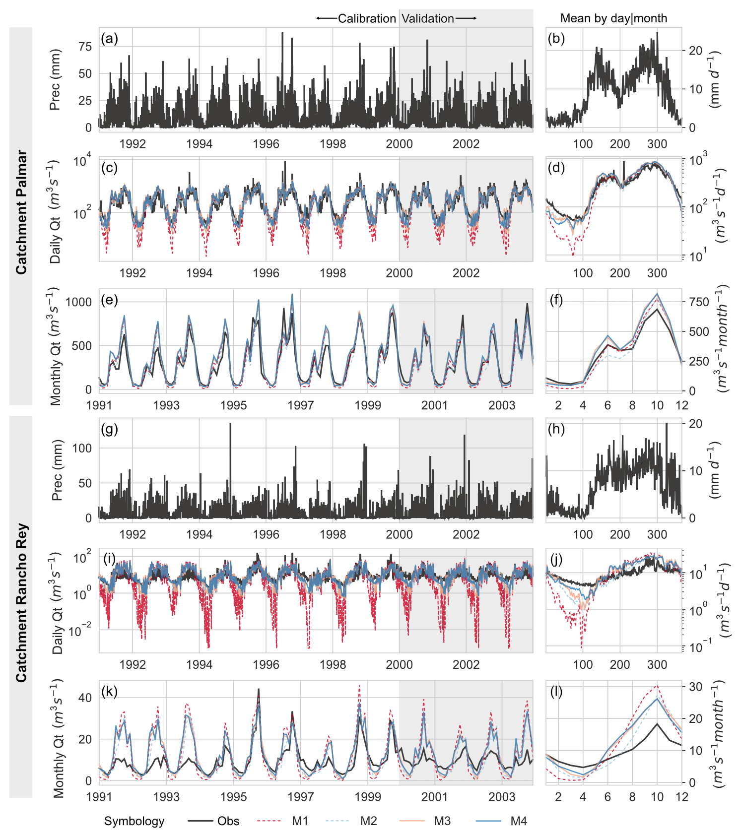
Figure 8 Simulated versus observed time series for catchments with the best streamflow KGE performance (Palmar watershed) and the worst streamflow simulation (Rancho Rey watershed). Black lines represent streamflow observations from 1990 to 2003. The panels on the right (b, d, f, h, j, l) show the mean daily and monthly time series.

The Palmar catchment exhibited acceptable performance (KGE > 0.5 and NSE > 0.45) for daily streamflow, but all configurations underestimated the highest peak flows during the calibration and validation periods. For the Rancho Rey catchment, the observed highest peak flows during 1997 were 3 times larger than simulated peak flows. Underestimation of simulated peak flows was related to the poor capabilities of CHIRPSc to detect heavy storms since observed peak flows were not associated with large precipitation amounts (Fig. 8a). In the Palmar and Rancho Rey catchments, the baseline (M1) underestimates low flows by 1 and 2 orders of magnitude during the dry season, respectively (Fig. 8d and j). Moreover, daily streamflow for M2 exhibited a mean relative bias (Eq. 17) of −0.046 with respect to M1 due to the underestimation of peak flows in all monitored catchments, and M3–M4 showed a mean relative bias of 0.156. The mean relative bias with respect to baseline (M1) using the logarithm of daily streamflow ranged from 0.24 to 0.29; hence, configuration M1 tended to generate lower flows during the dry period.

At a monthly scale, streamflow was preserved by the model configurations in several catchments, except for Rancho Rey, where simulated streamflow was on average 2 times larger than the observed streamflow during the rainy season (Fig. 8l). Such overestimation indicated that the bias factor was insufficient to correct the global precipitation product or for large discharge measurement errors. Furthermore, all configurations reproduced the seasonality of AET and PET from MODIS (not shown), but M3 and M4 underestimated the AET and PET in Palmar while showing good performance for AET in Rancho Rey. Moreover, simulated monthly soil moisture (SM) content was independently compared with the catchment average soil moisture content from the Land Parameter Retrieval Model (LPRM; Owe et al., 2008) product for the period 2012 to 2016. The simulated SM for M1 followed the seasonal behavior of the LPRM product in the Palmar catchment, matching the absolute LPRM % SM content. The LPRM product uses SM from the upper 5 cm against the 50 cm of the upper layer defined for all model configurations. However, all model configurations show a high correlation (CC > 0.7) in both catchments (Palmar and Rancho Rey), matching the seasonality.

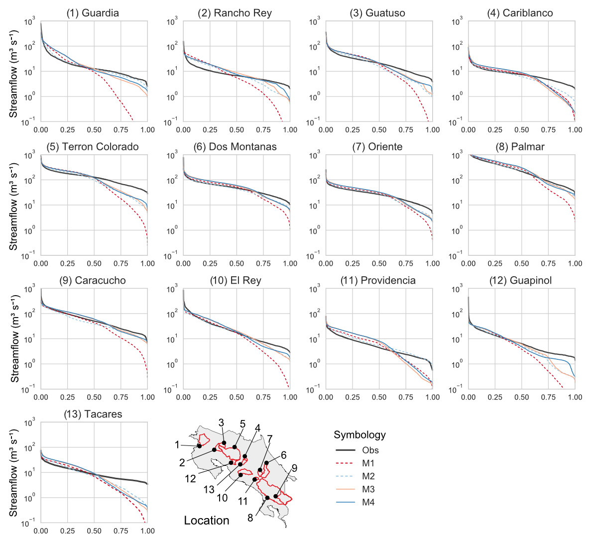
Figure 9 A comparison of observed flow duration curves (FDCs) as a hydrological signature and the matching simulated FDC for each model configuration. The simulated period was from 1991 to 2003.

The observed and simulated flow duration curves for all monitored catchments are shown for the period 1991–2003 in Fig. 9. The baseline (M1, dashed red line) underestimated the median and low flows in several catchments (Guardia, Rancho Rey, Guatuso, Terron Colorado, Caracucho, El Rey, Guapinol), with a median RMSE of 1.15 considering all monitored catchments, 2 times larger than other model configurations. M2 (dashed blue line) exhibited the best performance for median and low flows (with a median RMSE of 0.42), whereas M3 (orange line) and M4 (blue line) showed similar results to M2. Higher efficiencies for median and low flows were obtained for catchments that exhibited higher cross-correlation with precipitation (Fig. 4b), as was the case for Palmar, Caracucho, and El Rey, among others.

The simulated and observed hydrological signatures are shown in Fig. 10, where simulations covered the period 1991–2014, and observations covered different periods depending on available records. The comparison of hydrological signatures by monitored watershed is shown in Tables S1 and S2 in the Supplement. The simulated long-term mean annual water balance ($\mathrm{Prec}-Q_t-\mathrm{AET}$) was mostly closed in all catchments (∼0 mm), with average values of −1.80 mm (M1), −0.62 mm (M2), −0.79 mm (M3), and −1.17 mm (M4); hence the water balance was significantly improved when compared to the observed water balance. Indeed, the observed water balance ($\mathrm{Prec}-Q_t-\mathrm{AET}$) yielded values from −800 to 600 mm. Such variability in observed water balances may be related to the short common period of data but also to the discrepancies between the data sources (in situ, interpolated and merged, remotely sensed), as can be observed in Fig. S4. Figure S4 shows how the long-term water balance using the observed data differs from the Budyko curve in all monitored catchments (Westerberg et al., 2014), while the simulations fit the theoretical curve.

Figure 10 Observed and simulated spatial distribution of hydrological signatures. BFI: baseflow index (baseflow/streamflow), EI: evaporative index (AET/P), AI: aridity index (PET/P). Signatures from observations were obtained for the periods 2000–2003 (balance), 1991–2003 (BFI, SC), and 2002–2014 (EI, AI). Signatures from the simulations were obtained for the period 1991–2014, and the mean ± SD are shown on the lower left of each panel.

The spatial distribution of baseflow indices (BFI) derived from M2, M3, and M4 exhibited similarities with respect to the observations. Simulated BFI showed an overwhelming groundwater contribution to streamflow with relatively similar average values of 0.70, 0.69, 0.68, and 0.74 for model configurations M1, M2, M3, and M4, respectively.

Larger differences were observed in the northwest and southwest when comparing the BFI of M1 with respect to other configurations, whereas M4 resulted in larger contributions of baseflow to streamflow in coastal areas of the Caribbean. Similar spatial patterns were obtained for the streamflow coefficient ($\mathrm{SC}=Q_t/\mathrm{Prec}$), with low values in the drier northwest and higher values for catchments that receive more rainfall (Fig. 1e). In contrast, M2 indicated that a lower amount of precipitation became streamflow, with an average value of 0.49, in comparison with M1, M3, and M4, which showed medians of 0.52, 0.57, and 0.57, respectively. Moreover, M1 and M2 followed the spatial patterns of the observed SC due to their higher streamflow performance.

The EI and AI were similar for M3 and M4 due to their similar model parameters. The spatial distribution of observed EI from MODIS was reproduced by M3 and M4, whereas AI spatial patterns were preserved by M1. In addition, M1 and M3–M4 showed similar spatial patterns for EI and AI across the north, but differences were observed in the south, where M1 indicated lower water availability attributed to higher evaporative ratios (higher EI). M2 simulated the driest catchments, with an average value of EI and AI of 0.50 and 0.63, respectively, whereas M1 showed median values of 0.47 and 0.59, and M3–M4 values of 0.42 and 0.51.

5 Discussion

5.1 Remote sensing and global products as model forcings and calibration series

Daily precipitation from CHIRPS was preferred over other global precipitation products because of a relatively higher spatial resolution and good performance across different climates and biomes (e.g., Bayissa et al., 2017; Ullah et al., 2019; Zambrano-Bigiarini et al., 2017). Nevertheless, CHIRPS showed a large bias and more rainy days with respect to ground precipitation across Costa Rica (Fig. 4a). The results suggested that at large scales, the precipitation bias was compensated for since the mean bias factor (BF) was ∼1, but underestimation of precipitation was observed in mountainous regions as wells as large overestimations in the drier northwest (Fig. 4). Similarly, results from Chile by Zambrano-Bigiarini et al. (2017) indicated that an evaluation and even correction of global products is necessary and may be related to the poor density of ground gauges used to generate CHIRPS in those regions, especially across regions with steep topography (Funk et al., 2015). The latter authors also reported underestimation during extreme rainfall events and overestimation during rainy days.

Our simple, linear bias correction of CHIRPS showed better performance at monthly and annual scales and solved the water balance inconsistencies of most catchments (Fig. 10). However, the cross-correlation between daily precipitation and streamflow remains unchanged by the bias correction. Not surprisingly, our results showed that catchments with highly correlated streamflow and daily precipitation exhibited better performance than catchments with low correlations. Several studies highlighted those meteorological forcings are the largest source of uncertainty in hydrological modeling (e.g., Arheimer et al., 2020; Dal Molin et al., 2020; Lin et al., 2018; Wörner et al., 2019), whereas more complex bias correction techniques (e.g., quantile mapping) may improve the results (e.g., Goshime et al., 2019; Wörner et al., 2019). However, the lack of matching daily streamflows with precipitation inputs and intense rain events might persist. Nonetheless, Infante-Corona et al. (2014) suggested that global products can achieve better streamflow simulation results than sparse ground precipitation data, whereas Westerberg and Birkel (2015) found that in situ precipitation in Costa Rica may require corrections to achieve better model results.

The global CPC temperature dataset used was not bias-corrected due to the lack of sufficient in situ measurements. Temperature can introduce large errors in hydrological simulations if used for the estimation of potential evapotranspiration and actual evapotranspiration (Andersson et al., 2015). We corrected the temperature data set using elevation and a lapse rate parameter (Eq. 6) during the calibration steps. The corrected temperature closely followed the environmental lapse rate of 6 ^∘C temperature decrease per 1000 m elevation gain and improved model performance (KGE) by on average ∼10 %. Global evapotranspiration estimates showed differences compared to ground estimations in different regions due to the influence of, e.g., irrigation, vegetation dynamics, and uncertainty in climatological forcings (Pan et al., 2020; Velpuri et al., 2013). We used the PET and AET from MODIS 16 for calibration and evaluation due to the good performance reported in different applications around the world (e.g., Lin et al., 2018; Mu et al., 2013; Pan et al., 2020; Rajib et al., 2018b; Tang et al., 2011; Velpuri et al., 2013). Nevertheless, MODIS AET has shown poor performance at the point scale in different regions (e.g., Liu et al., 2015; Weerasinghe et al., 2020), but better performance when aggregated at the catchment scale (Velpuri et al., 2013). Additionally, Wohl et al. (2012) recognized that dense vegetation and frequent cloudiness in the humid tropics are challenges for satellite monitoring of AET. Unfortunately, the low density of eddy covariance towers and lack of comparative studies for tropical climates are limiting factors in the validation of MODIS 16 in Central America. Nonetheless, among the few existing studies available, Esquivel-Hernandez et al. (2017) compared the MODIS 16 PET product against 10 Priestley–Taylor station data-derived PET estimates in Costa Rica and found relatively small errors from −0.33 to +0.36 mm yr⁻¹.

5.2 HYPE performance in data-scarce tropical catchments

Simulated daily streamflow showed reasonable performance using the four model configurations, where M2 (calibrated Q_t monthly + Q_t daily) improved low flows simulations in comparison with M1 (Fig. 9). Moreover, our configuration using a step-wise calibration for Costa Rica resulted in improved streamflow performance compared to the global model by Arheimer et al. (2020). The main shortcomings of the four configurations were the underestimated larger peak flows (Fig. 8), but such errors were associated with the precipitation input rather than model capabilities. The spatial comparison of streamflow simulations indicated that catchments in the southwest performed best (KGE > 0.5 and NSE > 0.45, Fig. 6) compared to other areas. The southwestern Pacific is characterized by moderate precipitation seasonality (Fig. 1d) with a low bias in the precipitation product (Fig. 4a) and better performance in detecting rainy and dry days (Fig. S2), compared with the tropical climate gradient of the dry to humid tropics in Costa Rica. Furthermore, we found overestimated monthly streamflows in the drier northwestern region of Costa Rica (Rancho Ray and Guardia catchments with higher mean daily and monthly simulated streamflows, as is shown in Table S2). Previous studies have noted that HYPE overestimates streamflow in dry environments (Arheimer et al., 2020). Finally, the streamflow overestimation could also be related to the precipitation bias of CHIRPSc and possibly to the nonuniform spatial distribution of our streamflow observational sample, with additional “wetter” catchments used for calibration. Indeed, despite bias correction, precipitation overestimation persisted in drier environments (Fig. 4), associated with the lack of ground precipitation records to correct the CHIRPS product in headwater catchments, such as Rancho Rey. Furthermore, the low correlation of daily precipitation of CHIRPS with rain gauges resulted in low NSE values (<0.2) for daily streamflow due to the unsynchronized peak flows, mainly in the Caribbean slope.

Results from the Kruskal–Wallis test suggested median KGE in AET and PET from M3–M4 were statistically different compared to the baseline configuration M1 (the statistic H∼183 and p value < 0.05 for AET, and H∼72 and p value < 0.05 for PET). Nevertheless, the Kruskal–Wallis and Mann–Whitney tests indicated that median and the distribution of KGE for daily and monthly streamflows are similar among all model configurations (p values > 0.05). Hence, statistical significance using AET and PET for calibration is related to improvements in water partitioning in soil layers (Figs. 6 and 7) rather than runoff generation.

Such multi-objective calibration trade-offs were previously observed by, e.g., Zhang et al. (2018). Larger improvements were obtained for AET simulation of M3 and M4, whereas M1 (only daily Q_t calibration) showed similar PET performance in both periods (calibration and validation). The worst PET and AET simulations were observed for M2, since the monthly aggregation ignores an accurate representation of spatial water partitioning to match the monthly hydrograph (Rajib et al., 2018b). Our results also suggested that low flows were improved using PET and AET for calibration (Fig. 9), where FDC exhibited an average RMSLE (Eq. 16) value of $\sim \mathrm{0.5}\pm \mathrm{0.22}$ compared to 1.1±0.53 from M1, constraining vertical fluxes and regulating discharge from soil layers (Massari et al., 2015; Rakovec et al., 2016). The constrained posterior parameter distributions using MODIS PET, and AET in calibration steps decreased the variability of parameters related to evapotranspiration processes (lp, cevpam). However, the soil water content parameters (wcfc, wcwp, wcep) ranges were similar among model configurations (Fig. 7). Additionally, including monthly Q_t into the calibration routine also constrained parameters related to soil layer discharge (srrate, rrcs1, rrcs3) for the most frequent soil types on the monitored catchments. Such results highlight that remotely sensed PET and AET are useful at constraining some parameters and that the combination of data sources representing different modeled hydrological processes helps constrain model uncertainties, particularly for large-scale domains (Rajib et al., 2018b). Despite the partly different calibration periods used due to the limited data availability, similar record lengths (8 years of calibration and 3 years of validation) resulted in consistent results from M1 to M4.

Despite the generally reasonable performance of our model configurations, we found some issues when comparing our results with previous efforts, such as those of Birkel et al. (2012), who modeled the streamflow in the Sarapiqui River basin (data not used in this study for calibration) with the HBVlight model (Seibert, 2005) for the period from 1983 to 1991 and obtained an NSE of 0.74 after rainfall correction of the underestimated observed precipitation. Our configuration M4 resulted in an NSE = −5.6 due to rainfall underestimation (Frumau et al., 2011). In contrast, our model configuration M4 showed lower improvements with respect to the global product of Arheimer et al. (2020). For example, we obtained a KGE = 0.73 and NSE = 0.46 for the streamflow simulation of the Palmar catchment, in comparison to the global product showing a KGE of less than 0.3. Such results reflect that more data are required to improve the streamflow response at local scales.

5.3 Independent model evaluation using hydrological signatures

A hydrological model useful for water management should be able to mimic streamflow seasonality and to realistically represent the large-scale physical processes of the water partitioned by vegetation interception and the soil matrix into evapotranspiration and discharge (Arheimer et al., 2020; Kwon et al., 2020; Pechlivanidis and Arheimer, 2015; Rajib et al., 2018b; Rakovec et al., 2016; Xiong and Zeng, 2019). We, therefore, independently evaluated the four configurations using a range of hydrological signatures (Table 4) following Westerberg and McMillan (2015) in an attempt to single out the sought-after well-balanced model for use in decision-making. However, using multiple signatures also complicated the interpretation of simulations since daily streamflow ($Q_{t_{\mathrm{d}}}$) and monthly streamflow ($Q_{t_{\mathrm{m}}}$) indicated improvements in different configurations (see Tables S1 and S2).

Significant spatial variations in hydrological signatures were observed between M1–M2 and M3–M4 since implementing a spatial calibration of AET improved the representativeness of the more complex large-scale climate gradient. Similar results were found in catchments in the United States (Lin et al., 2018; Rajib et al., 2018a) and worldwide (Arheimer et al., 2020). The model configurations M3 and M4 better reproduced the spatial variability between the Pacific and Caribbean basins and the north–south gradient of the AI and EI (Esquivel-Hernandez et al., 2017). Furthermore, the resulting hydrological signatures of M3 and M4 were consistent with previous small catchment-scale studies that showed that runoff coefficients tend to be larger than the evaporative index (Dehaspe et al., 2018; Gómez-Delgado et al., 2011). Results also suggested that the event streamflow response is dominated by quick near-surface soil water discharge (Dehaspe et al., 2018), with streamflow being fed by groundwater during dry periods resulting in BFI values exceeding 0.7 (Birkel et al., 2012). In contrast to Westerberg et al. (2014), who calibrated Central American catchments using FDC information, we used the observed FDCs as an independent hydrological signature (Fig. 9). The configurations M2 to M4 outperformed the baseline (M1), supporting the notion that only streamflow used for calibration is not enough to produce a well-balanced model.

6 Conclusions

This study is the first attempt to apply the process-based, conceptual rainfall–runoff HYPE model at the national scale of Costa Rica (∼600 simulated catchments). Due to the lack of detailed observational data available for Costa Rica, as in most parts of the world's tropics, we used different global topography, soil, land use products, daily streamflow from 13 gauges, the bias-corrected global precipitation product CHIRPS (with 75 ground stations) and remotely sensed MODIS 16 PET and AET products to improve the performance of HYPE in a step-wise calibration procedure towards a well-balanced model useful for water resources management. The calibrated model configurations were independently evaluated using a suite of hydrological signatures. We summarize our main findings here.

• Bias was observed in the precipitation from CHIRPS, with underestimation in mountainous regions and overestimation in the driest region with around 1000 mm of annual rainfall in Costa Rica.

• CHIRPS showed ∼10 % more days with rainfall in comparison with ground precipitation but could not capture extreme rainfall events, which ultimately impacts streamflow simulation.

• Our bias correction procedure using the linear-scaling technique reduced annual water balance inconsistencies ($\mathrm{Prec}<Q+\mathrm{ET}$) by 25 %. Still, a more complex methodology is required to improve daily precipitation depth and timing.

• The temperature could efficiently be used with an elevation correction; nevertheless, a higher-resolution temperature product or downscaling approach would improve the many micro-climates across the complex topography in Costa Rica.

• HYPE successfully reproduced major processes (evapotranspiration, runoff, baseflow discharge) of tropical catchments in Costa Rica, where we obtained acceptable performance for daily streamflow (median KGE from 0.4 to 0.6) and good performance for monthly streamflow (median KGE from 0.6 to 0.9, and median NSE from 0.4 to 0.55), with best-fit results for PET and AET of KGE = 0.6 and KGE = 0.5, respectively.

• Model calibration using monthly and daily streamflow (M2) improved the performance of the low flows in comparison to only daily streamflow (M1) calibration, where the average RMSLE of FDC was computed as 0.42±0.22 for M2, compared to 1.14±0.53 from M1.

• Remotely sensed PET and AET constrained the soil type and land cover parameters associated with the evapotranspiration process.

• Statistical differences in AET and PET performance was observed for M3–M4 with respect to M1 and M2, but not for daily and monthly (KGE) streamflow simulations.

• Including PET and AET in calibration (M3 and M4) slightly decreased the overall streamflow performance (average KGE of 0.47±0.17 compared to 0.54±0.09 from baseline M1) at the expense of an improved and more well-balanced median and low flow (average RMSLE for FDC of $\sim \mathrm{0.5}\pm \mathrm{0.22}$ compared to 1.1±0.53 from baseline M1) simulation and evapotranspiration water partitioning.

• Simulated hydrological signatures (aridity index, evaporative index, baseflow index, streamflow coefficient, flow duration curve) differed for each calibrated model, but configurations M3 and M4 more realistically mimicked the spatial distribution of all tested hydrological signatures.

We conclude that M3 and M4 are promising model configurations for the quantitative assessment of water resources in Costa Rica and that PET-AET and daily streamflow (M3) and PET-AET, and daily and monthly streamflow (M4) represent an appropriate calibration sequence for regional modeling. Improvements to these models could be achieved by incorporating more independent data into the calibration process, such as soil moisture and groundwater level and storage data. However, all global products crucially depend on evaluation and even correction, which require observational in situ data. Nonetheless, we hope to have provided a way forward towards a large-sale operational hydrological model for the humid tropics of Costa Rica and potentially for other humid regions of the world.