the Creative Commons Attribution 4.0 License.
the Creative Commons Attribution 4.0 License.
 | 18 Feb 2022
Historical simulation of maize water footprints with a new global gridded crop model ACEA
Joep F. Schyns
Martijn J. Booij
Rick J. Hogeboom
Crop water productivity is a key element of water and food security in the world and can be quantified by the water footprint (WF). Previous studies have looked at the spatially explicit distribution of crop WFs, but little is known about their temporal dynamics. Here, we present AquaCrop-Earth@lternatives (ACEA), a new process-based global gridded crop model that can simulate three consumptive WF components: green (WFg), blue from irrigation (WFbi), and blue from capillary rise (WFbc). The model is applied to analyse global maize production in 1986–2016 at 5×5 arcmin spatial resolution. Our results show that over the 2012–2016 period, the global average unit WF of maize is 728.0 m3 t−1 yr−1 (91.2 % WFg, 7.6 % WFbi, and 1.2 % WFbc), with values varying greatly around the world. Regions with high-input agriculture (e.g. Western Europe and Northern America) show small unit WFs and low interannual variability, while low-input regions show opposite outcomes (e.g. Middle and Eastern Africa). From 1986 to 2016, the global average unit WF reduced by a third, mainly due to the historical increase in maize yields. However, due to the rapid expansion of rainfed and irrigated areas, the global WF of maize production increased by half, peaking at 768.3×10⁹ m3 yr−1 in 2016. As many regions still have a high potential in closing yield gaps, unit WFs are likely to reduce further. Simultaneously, humanity's rising demand for food and biofuels may further expand maize areas and hence increase WFs of production. Thus, it is important to address the sustainability and purpose of maize production, especially in those regions where it might endanger ecosystems and human livelihoods.
- Article
(3786 KB) - Full-text XML
-
Supplement
(1615 KB) - BibTeX
- EndNote


Ever-increasing crop production is one of the reasons why humanity transgresses planetary boundaries (Campbell et al., 2017; Jaramillo and Destouni, 2015). In particular, crop production is estimated to account for around 87 % of humanity's total water consumption (Hoekstra and Mekonnen, 2012), which in some places already exceeds environmental limits, endangering local ecosystems and water security (Hoekstra et al., 2012b; Schyns et al., 2019; Verones et al., 2017). Moreover, the situation is likely to worsen in the future as crop water consumption continues to grow (Wada and Bierkens, 2014; Greve et al., 2018).
One way to minimise crops' pressure on water resources is to increase crop water productivity, i.e. have “more crop per drop” (Giordano et al., 2006). The volume of water needed to produce a unit of a crop can be measured by the consumptive water footprint (WF). It is calculated as the crop water use (CWU) over crop yield (Hoekstra, 2011). CWU reflects the amount of accumulated evapotranspiration (ET) over the growing season and can be attributed to green (from precipitation) and blue water (from capillary rise – CR – and irrigation). Crop yield reflects the harvestable part of crop biomass.
Since its introduction in 2002, the WF concept has been widely applied to analyse crop water productivity (Feng et al., 2021; Lovarelli et al., 2016). However, most studies either focus on a small geographical extent (e.g. specific catchments or administrative units) or consider a short time period. The few existing global studies focus on the average year 2000 (Mekonnen and Hoekstra, 2011; Siebert and Döll, 2010; Tuninetti et al., 2015) and thus lack the analysis of historical trends and interannual variability. Moreover, their methods to estimate green and blue crop WFs have several limitations: (i) the applied crop water requirement approach does not simulate crop growth and its response to thermal stresses; (ii) the water balance is simulated without considering CR that can be relevant in areas with shallow groundwater (Hoekstra et al., 2012a); (iii) the green–blue water partitioning is performed in post-processing, which does not account for the full dynamics of green and blue water fluxes in the soil water balance (Hoekstra, 2019). Alternatively to these studies, crop WFs can be simulated with global gridded crop models (GGCMs). These models (e.g. LPJmL, EPIC, and DSSAT) typically simulate crop growth and water use from the underlying biophysical processes in the atmosphere–plant–soil continuum in each grid cell (Müller et al., 2017). Due to high computational demands, a limited body of literature applies GGCMs. The most prominent studies come from the Global Gridded Crop Model Intercomparison (GGCMI) within the Agricultural Model Intercomparison and Improvement Project (Rosenzweig et al., 2013; Elliott et al., 2015) that mainly uses ensembles of GGCMs to analyse climate change impacts on crop production (Ruane et al., 2018; Jägermeyr et al., 2021a; Minoli et al., 2019; Zabel et al., 2021; Deryng et al., 2016). Besides GGCMI, several studies look into spatial patterns of crop water productivity but not into historical dynamics (Liu et al., 2009, 2016; Fader et al., 2010).
In this paper, we present AquaCrop-Earth@lternatives (ACEA) – a global gridded version of FAO's water-driven, process-based, and site-based crop growth model AquaCrop (Vanuytrecht et al., 2014; Steduto et al., 2009). We use AquaCrop because it requires a small number of inputs to produce reliable estimates of crop yield and CWU under various agro-climatic conditions (Araya et al., 2016; Greaves and Wang, 2016; Karandish and Hoekstra, 2017; Maniruzzaman et al., 2015; Chukalla et al., 2015; Zhuo et al., 2016). In recent years, several studies applied it at the regional scale via GIS software (Lorite et al., 2013; Huang et al., 2019; Han et al., 2020). However, in this implementation, AquaCrop demands inputs for each simulation site in separate files, which can be computationally inefficient. To overcome this limitation, ACEA utilises the open-source version developed by Kelly and Foster (2021) – AquaCrop-OSPy. We optimise ACEA for large-scale simulations by minimising the number of input files and by parallelising the modelling procedure. Furthermore, we implement the daily accounting of green and blue water fluxes in the soil profile, including CR contributions from shallow groundwater.
Although ACEA can be applied to simulate all crops that are compatible with AquaCrop, we demonstrate ACEA's performance by simulating global WFs of maize (Zea mays L.) at 5×5 arcmin resolution (∼8.3 km × 8.3 km). We cover the 1986–2016 period, considering historical changes in harvested areas and crop yields. We focus on maize because of several reasons. First, it is the most produced grain in the world (FAOSTAT, 2021). Second, it plays a major role in the global economy by being used not only as food for animals (including humans), but also to produce biofuels and other biochemicals (Ranum et al., 2014). Finally, maize WFs are not as extensively researched as WFs of other major grains, such as rice and wheat (Chapagain and Hoekstra, 2011; Mekonnen and Hoekstra, 2010). In our analysis, we reveal temporal and spatial patterns in both unit WFs of maize (in m3 t−1 yr−1) and WFs of maize production (in m3 yr−1) at global and regional levels. We conclude by comparing our results to estimates from previous studies, discussing both limitations and advantages of crop water productivity analysis with ACEA, and addressing the sustainability of maize production.
2.1 Global gridded crop model ACEA
2.1.1 General description
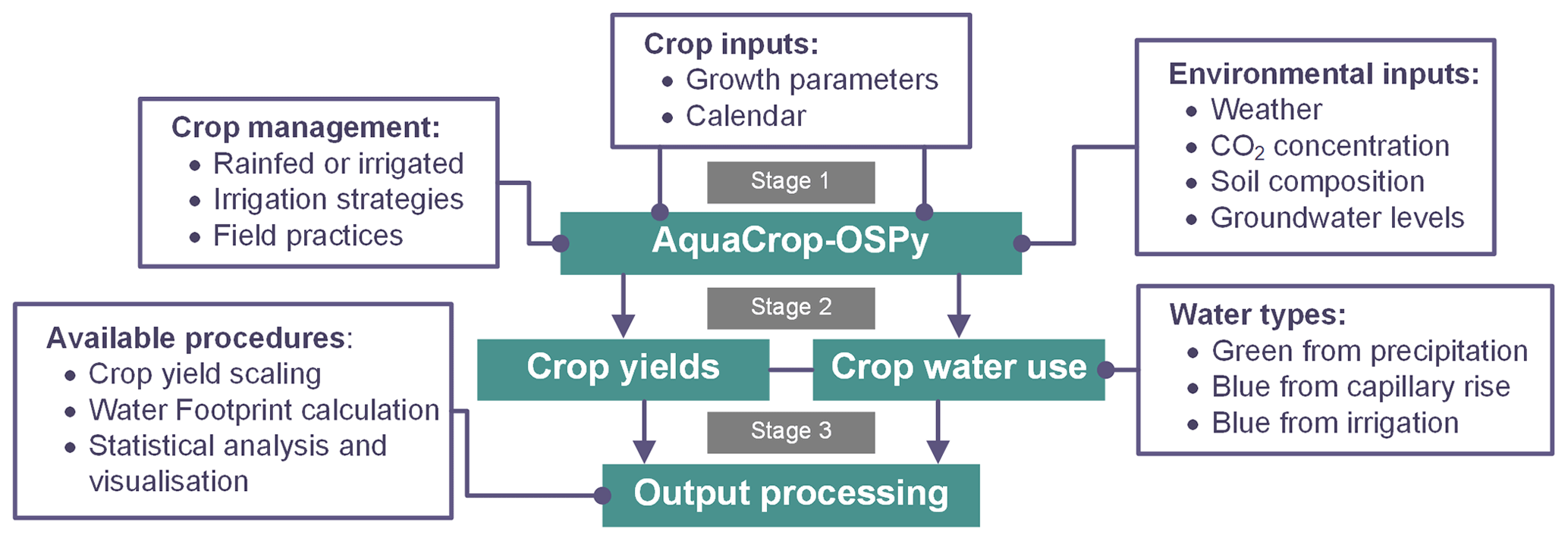
ACEA is written in Python, and its simulation procedure has three main stages as shown in Fig. 1. In the first stage, ACEA collects crop and environmental input data for each grid cell within the study area (elaborated in Sect. 2.2). The spatial resolution of input data determines the size of grid cells, while the geographical extent of rainfed and irrigated production systems determines the number of cells. Depending on water availability, several rainfed and irrigation setups can be selected. The rainfed setups include fully rainfed (s1) and rainfed with presence of shallow groundwater (s2). The irrigation setups include surface irrigation (s3), sprinkler irrigation (s4), drip irrigation (s5), and surface irrigation with presence of shallow groundwater (s6). Besides water availability setups, crop management can be customised by selecting field practices (mulches, weed control, and bunds) and adjusting irrigation strategies. In the second stage, ACEA runs AquaCrop-OSPy (described in Sect. 2.1.2) in each grid cell independently, meaning that lateral processes, such as water inflow from adjacent cells, are not considered. Main output variables are crop yield and CWU (see all outputs in Sect. S1.1 in the Supplement). In the third stage, ACEA aggregates the raw outputs from each grid cell into global gridded datasets in NetCDF format. Then, it runs optional post-processing procedures, including crop yield scaling (see Sect. 2.1.4), WF calculation (Sect. 2.1.3), statistical analysis (Sect. 2.1.5), and visualisation.
2.1.2 AquaCrop-OSPy and green–blue water accounting
We use AquaCrop-OSPy (Kelly and Foster, 2021), which is a Python implementation of FAO's AquaCrop application version 6.1. This crop model uses crop, soil, climate, field, and irrigation management data (see Fig. 1) to simulate daily crop growth and the soil water balance (Vanuytrecht et al., 2014). The latter includes water input (precipitation, irrigation, and CR) and output (runoff, evaporation (E), transpiration (T), and deep percolation) fluxes as well as upward and downward fluxes between soil compartments (see Fig. 2). Crop growth is temperature-driven via growing degree days (GDDs) and expressed by the variable effective rooting depth and canopy cover. Canopy cover is used to convert the potential evapotranspiration (ET0) into T, which drives dry above-ground biomass growth via a CO2-adjusted water productivity factor. At the end of the growing season, the accumulated biomass is converted into a dry crop yield via a harvest index. The crop growth is affected by thermal and water stresses. For example, the latter can induce stomatal closure and constrain canopy expansion, which would lead to reduced T and biomass growth. Note that the nutrient cycle and water salinity are not simulated in AquaCrop-OSPy. For more information on AquaCrop, please refer to user manuals (Raes et al., 2009; Steduto et al., 2009; Hsiao et al., 2009).
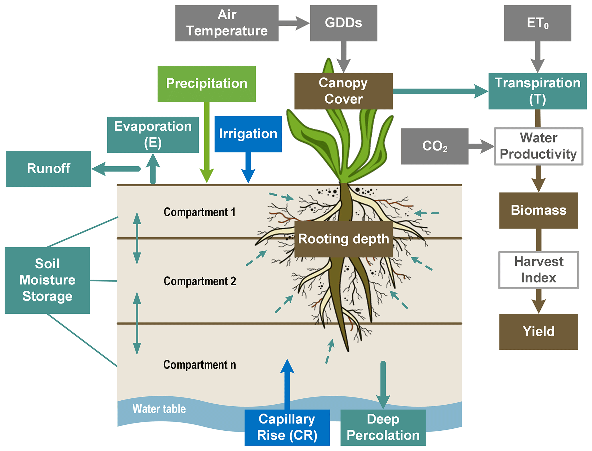
Figure 2AquaCrop simulation scheme. Green, blue, and cyan boxes represent variables related to the soil water balance, brown boxes to crop growth, and grey boxes to climate. We only abbreviate the terms that are often used in the text.
The green–blue water accounting is our most important addition to the AquaCrop-OSPy code (see other changes in Sect. S1.2). According to Hoekstra (2019), each of the input fluxes is attributed to one of the three water types: green from precipitation, blue from CR, or blue from irrigation (see the respective coloured boxes in Fig. 2). Once entered, these fluxes are assumed to mix evenly with moisture in soil compartments at the top or the bottom of the soil profile. Then, the mixed water is partly redistributed via the upward and downward fluxes between the compartments due to gravitational and capillary forces. The mixed water is taken up for ET – from the upper part of the soil profile for E and from all compartments within the effective rooting depth for T. Therefore, the volumes of the three water types stored in each soil compartment constantly change. This implies that the composition of ET varies per day too, and, consequently, we can estimate precise CWU for each of the three water types. For more details about green–blue water accounting, please refer to Hoekstra (2019).
2.1.3 Water footprint calculation
ACEA calculates the annual consumptive unit WF (m3 t−1 yr−1) of a crop as the sum of three WF components (Hoekstra, 2011):
where WFg is the green WF, WFbc is the blue WF from CR, and WFbi is the blue WF from irrigation. Each unit WF component is calculated as the crop water use CWUx (mm yr−1) of a water type x (g, bc, or bi) over crop yield Y (t ha−1 yr−1). To convert from millimetres per year (mm yr−1) into cubic metres per hectare per year (m3 ha−1 yr−1), CWUx is multiplied by 10:
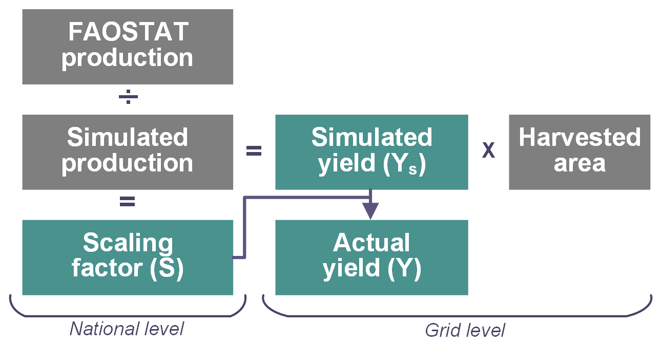
To obtain Y, the simulated crop yield Ys in AquaCrop-OSPy is corrected by two unitless coefficients. The first one is a conversion coefficient from dry to fresh crop yield Kf (0.87 for maize); the second one is a yield scaling factor S, which is introduced to account for external developments not modelled in ACEA (explained in Sect. 2.1.4):
The simulated water availability setups are combined to analyse rainfed and irrigated production systems. In the case of rainfed systems, unit WFs of a water type x from setups s1 and s2 (defined in Sect. 2.1.1) are simply summed as rainfed grid cells always only have one setup. On the other hand, in irrigated systems, the same grid cell can have several irrigated setups (s3 to s6) at once. Therefore, irrigated unit WFs are multiplied by irrigation factor Ki before being summed. The latter reflects a fraction of irrigated area under the respective irrigation method obtained from Jägermeyr et al. (2015):
Note that we differentiate between the unit WF and the WF of crop production. The latter is calculated by multiplying the unit WF by the annual crop production, and thus it is measured in cubic metres per year.
2.1.4 Crop yield scaling
During the last decades, maize yields have increased globally due to various long-term agricultural developments, namely advances in agricultural inputs (e.g. irrigation, fertilisers, machinery, and chemical control of weeds and insects) and better crop varieties (e.g. higher plant density and improved biotic and abiotic stress resistance) (Duvick, 2005; Lorenz et al., 2010). At the same time, there have been short-term developments that caused interannual variability in maize yields, namely disruptions due to political (e.g. civil wars), economic (e.g. food prices), and natural reasons (e.g. locust plague, flooding) (Woo-Cumings, 2002; Smale et al., 2011). Both long-term and short-term developments are not modelled in ACEA, either because of input data limitations or because required processes are not included in AquaCrop-OSPy. However, following the logic of previous studies (Mekonnen and Hoekstra, 2011; Siebert and Döll, 2010), we attempt to represent the combined effect of these developments via yield scaling factors (S) that scale Ys to the annual statistics from FAO (FAOSTAT, 2021).
Because FAO reports the total crop production at the national scale, S values are the same for each grid cell within a country (see Fig. 3). S is calculated per country per year as the ratio of the official crop production PFAO (t yr−1) reported by FAO to the simulated crop production PACEA in ACEA. The latter is calculated as the sum of rainfed and irrigated production:
where Ys is the simulated crop yield (t ha−1 yr−1) in a specific water availability setup (rainfed: s1 and s2, irrigated: s3–s6), Arainfed and Airrigated are historical rainfed and irrigated harvested areas (ha yr−1), and Ki and Kf are defined in Sect. 2.1.3.
Interannual variability in S leads to interannual variability in crop yields and hence in unit WFs. However, we aim to capture the effect of long-term external conditions while maintaining the modelled climate-related interannual variability. Therefore, we take a 3-year moving average of scaling factors for each country (using the previous, current, and next year's factors). This allows us to keep the overall trend and variability in historical crop yields while attenuating extreme responses to short-term external developments.
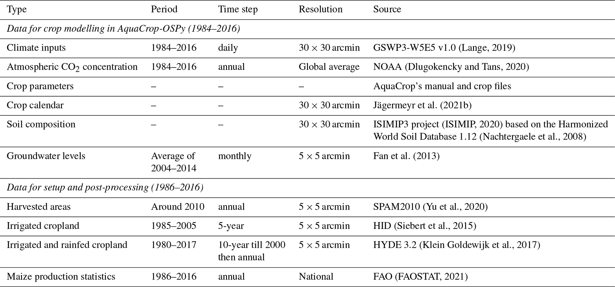
Table 1Summary of input data used for maize crop modelling and post-processing in ACEA.
One could argue that CWU should be scaled as well. However, we only scale Ys due to several reasons. First, improvements in crop varieties (e.g. angle and size of leaves) can change the ratio of T to E, but this has minor effects on CWU as an increase (or decrease) in T is compensated by a decrease (or increase) in E (Xu et al., 2018; Nagore et al., 2014). Both E and T consume green and blue water, and thus we do not expect major changes in green and blue CWUs either. Second, the historical increase in plant density mainly increases maize yields, while CWU values stay relatively similar for the same reasons as mentioned above. A sensitivity analysis with our model (see Sect. S1.3) confirms this. Third, an input of nitrogen fertiliser can marginally increase CWU when first applied, but additional fertiliser amounts would not always lead to a larger CWU (Rudnick et al., 2017). In our study, we have to assume no nutrient stress (i.e. optimal nutrient supply) as AquaCrop-OSPy cannot simulate the nutrient cycle. This might lead to an overestimation of CWU in places that do not use fertilisers. However, we assume that the majority of maize is produced by high-input farms with sufficient nutrient supply, and thus our CWU estimates over large scales should be hardly affected. To sum up, the literature indicates that historical changes in crop varieties and agricultural inputs only have minor effects on maize CWU compared to yields. Therefore, scaling the yields should be sufficient to represent historical dynamics in maize unit WFs.
2.1.5 Statistical analysis of results
Statistical analysis is performed at several spatial scales according to the UN classification (UNSD, 2021): global, (sub)regional, and national. To obtain representative values for each scale, unit WFs are averaged based on the production amounts, and related variables (Y, CWU, and S) are averaged based on the harvested area in each grid cell. We also focus on two timeframes: (i) the last 5-year period (2012–2016) as a proxy for the current state of unit WFs and (ii) the whole 1986–2016 period to analyse historical changes. For the trend analysis of WFs and related variables, we use the Mann–Kendall test, which identifies the direction and significance of a trend in time series (Hussain and Mahmud, 2019). We further detrend the variables with significant trends to analyse interannual variations by removing a linear trend. The interannual variability is measured by estimating the coefficient of variation (CV) of detrended time series, and the dependency between different variables is determined by the Pearson linear correlation coefficient (Brown, 1998).
2.2 Simulation setup
Data needed to run ACEA for global maize production are summarised in Table 1. We simulate maize WFs over the 1986–2016 period at 30×30 arcmin resolution (∼50 km × 50 km), which is also common for GGCMI studies (Franke et al., 2020). The maize-growing grid cells are selected according to the location of maize production systems obtained from SPAM2010 (Yu et al., 2020). Note that we do not differentiate between the various types of maize (e.g. pop, dent, flour, and sweet corns) due to a lack of input data. We consider only one growing season per year, as double cropping of maize is negligible at the global scale (Portmann et al., 2010). The periods between growing seasons are also simulated to account for soil moisture changes. We exclusively use water availability setups s1 to s4 (defined in Sect. 2.1.1), as s5 and s6 are not common for maize production. The 30×30 arcmin modelling outputs are distributed among its underlying 5×5 arcmin grid cells from SPAM2010, and hence the post-processing (see Sect. 2.1.1) is performed at 5×5 arcmin resolution.
Climate inputs for AquaCrop-OSPy are obtained from the bias-corrected reanalysis product GSWP3-W5E5 v1.0 (Lange, 2019) that provides historical daily rainfall, temperature, surface shortwave radiation, wind speed, and relative humidity. These variables (except rainfall) are used together with a global elevation model (Amante, 2009) to estimate ET0 according to the Penman–Monteith equation (Allen et al., 1998).
Crop parameters are obtained from the AquaCrop manual (Raes et al., 2018) and the default maize crop file provided with AquaCrop-OSPy. In the case of inconsistencies among these two sources, priority is given to data from the manual. The considered crop calendar (Jägermeyr et al., 2021b) is a composite of multiple recent data sources that rely on national and subnational statistics, remote sensing products, and modelling. The planting and harvest dates from the crop calendar are used to calculate GDDs with the third calculation method from AquaCrop (Raes et al., 2018). Crop development stages (in GDDs) for each grid cell are recalculated with the method of Minoli et al. (2019) to ensure that the average growing season duration is similar to the one from the crop calendar. Since some growing seasons are colder than average, they are allowed to be up to 15 % longer for the crop to reach maturity. Additional information on maize parametrisation is provided in Sect. S1.4.
The soil profile is defined as one layer of 3 m depth with eight compartments ranging from 0.1 to 0.7 m in thickness. The selection of soil compartments is based on the analysis described in Sect. S1.5. Sand, silt, and clay fractions for each grid cell are obtained from the ISIMIP3 project (ISIMIP, 2020) which provides the fractions from the Harmonized World Soil Database 1.12 (Nachtergaele et al., 2008) upscaled to 30×30 arcmin. The soil composition is then converted into hydraulic parameters using a pedotransfer function (Saxton and Rawls, 2006) included in AquaCrop-OSPy. To ensure realistic initial soil moisture values, we run the model 2 years in advance of our study period (described in Sect. S1.6).
The average monthly groundwater levels are taken from Fan et al. (2013) and initially upscaled to 5×5 arcmin using a resample function in QGIS (QGIS, 2021). Then, the near-surface values are lowered to 1 m depth under the assumption that farmers drain the agricultural field to avoid aeration stress (see Sect. S1.7). We further upscale monthly groundwater levels to 30×30 arcmin by taking an average over the underlying 5×5 arcmin grid cells where maize production and shallow groundwater (<3 m in depth) are present. Finally, we interpolate the monthly values to obtain daily groundwater levels. Note that Fan et al. (2013) report values in a natural state for only 1 year, and thus short- and long-term effects of groundwater pumping and natural annual fluctuations are not considered.
Following previous studies (Andarzian et al., 2011; Khoshravesh et al., 2013), irrigation events are triggered as soon as the soil moisture drops below 50 % of the maximum available soil water within the root zone. The amount of irrigated water in each of the irrigated setups is limited by field capacity and depends on the percentage of wetted area by the respective irrigation method (Chukalla et al., 2015). The conveyance efficiency is set to 100 % to provide the net irrigation requirement. No particular field management practices are activated due to a lack of data on where they are applied.
To account for the historical changes in harvested areas, we extrapolate SPAM2010 to the 1986–2016 period. The extrapolation is performed using two historical datasets on rainfed and irrigated cropland extent, i.e. HYDE 3.2 (Klein Goldewijk et al., 2017) and HID (Siebert et al., 2015), under the assumption that harvested areas of maize from SPAM2010 experienced the same dynamics as the croplands did. Then, the extrapolated areas are scaled to FAOSTAT (2021). A detailed description of the extrapolation and scaling procedures is provided in Sect. S1.8.
3.1 Average water footprints in 2012–2016
The global average unit WF of maize is 728.0 m3 t−1 yr−1 over the 2012–2016 period. The share of green water (WFg) is 91.2 %, while the shares of blue water from CR (WFbc) and irrigation (WFbi) are 1.2 % and 7.6 %, respectively. The unit WF has a distinct latitudinal distribution (see Fig. 4a) following the same patterns as crop yields (see Fig. S1a in the Supplement). High yields and small unit WFs north of 20∘ N are due to high-input production systems in the main maize-growing regions: Northern America (WF is 483.1 m3 t−1 yr−1; yield is 10.1 t ha−1 yr−1), Europe (597.5 m3 t−1 yr−1; 6.2 t ha−1 yr−1), and Eastern Asia (615.7 m3 t−1 yr−1; 5.9 t ha−1 yr−1). On the other hand, the regions with low yields have substantially larger unit WFs and are mostly located in arid parts of the world that mainly rely on low-input rainfed production systems (e.g. Middle and Eastern Africa).
Rainfed systems produce 76.5 % of maize and show on average a 10.5 % larger unit WF (744.9 m3 t−1 yr−1) than irrigated systems (674.1 m3 t−1 yr−1). However, both the smallest and the largest regional unit WFs (among regions with at least 0.5 % of global maize production) are located in areas dominated by rainfed production (see Table 2), with the largest one in Middle Africa (3157.9 m3 t−1 yr−1) and the smallest one in Western Europe (433.2 m3 t−1 yr−1). The smaller WF in the latter region can be explained by both a smaller CWU (i.e. lower ET rates) and a higher crop yield (see Fig. S1). The WF values also vary among areas dominated by irrigated production. For example, the WF in Western Asia (569.6 m3 t−1 yr−1) is almost half of that in Northern Africa (1035.5 m3 t−1 yr−1) due to a smaller CWU, while maize yields in both regions are similar. The global maps with separated rainfed and irrigated unit WFs can be found in Fig. S2.
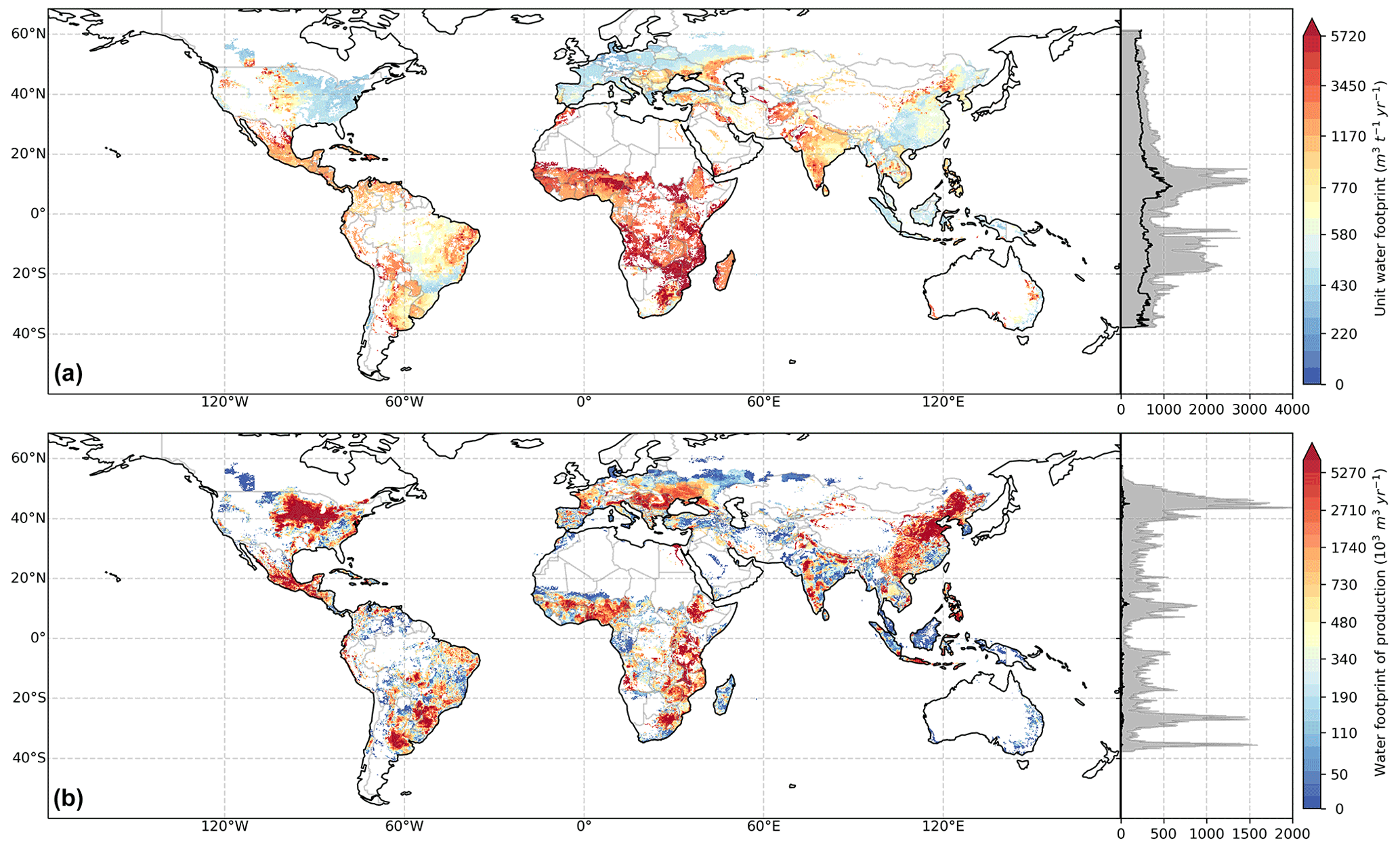
Figure 4Unit water footprint (a) (m3 t−1 yr−1) and water footprint of production (b) (103 m3 yr−1) of maize as the average over 2012–2016 at 5×5 arcmin resolution. The grey area in the side chart represents the median of all data points along the respective latitude, and the black line is the 10th percentile.
Table 2Overview of global maize production and water footprint statistics as the average over 2012–2016 (except the coefficient of variation (CV), which is estimated for 1986–2016). CWU is crop water use, and WF is water footprint (g – green, bc – blue from capillary rise, bi – blue from irrigation). The selection of regions is based on the UN classification (UNSD, 2021).
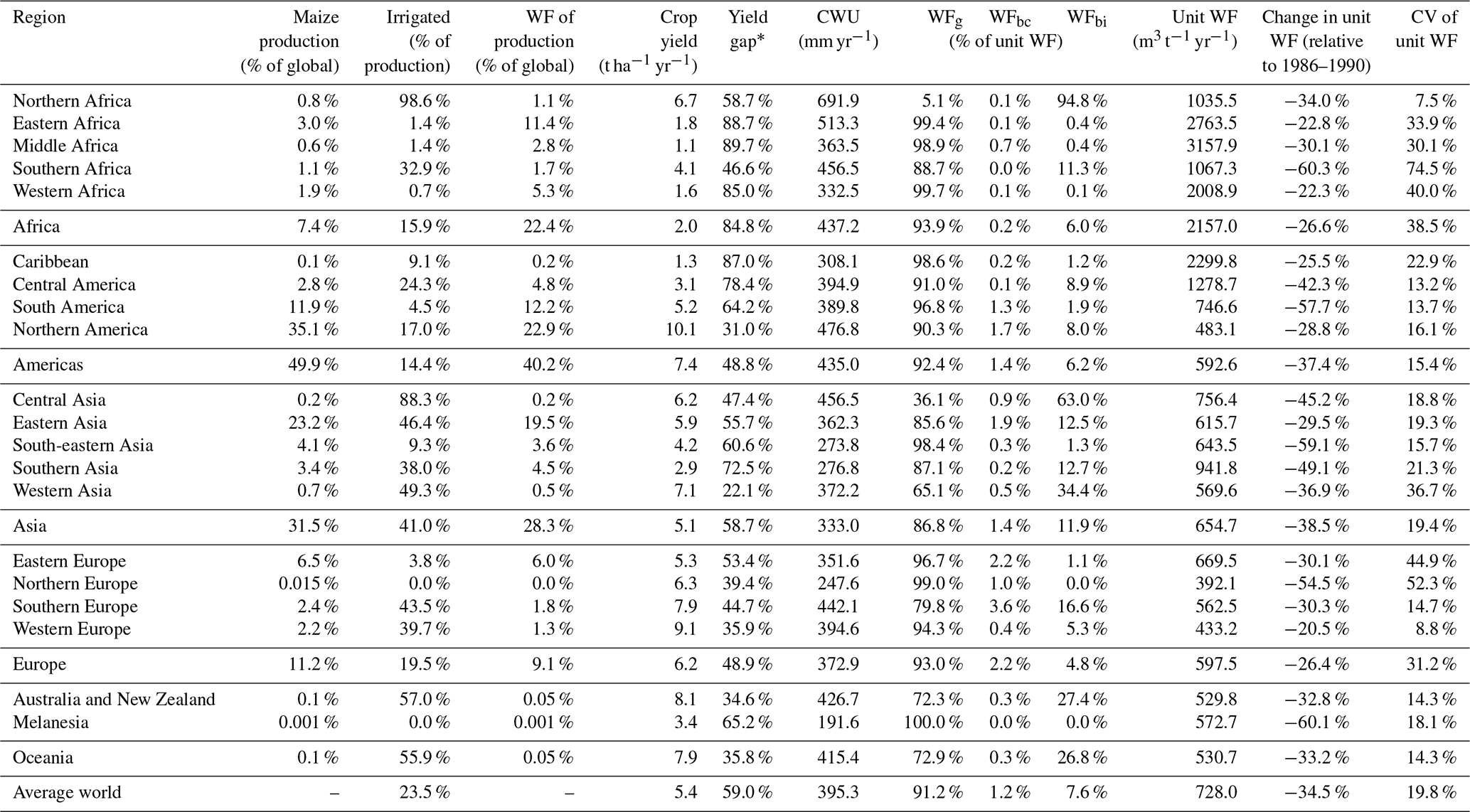
* Yield gap is estimated as 100 % – yield scaling factor.
Zooming to the national level, the average unit WF of the nine biggest producing countries plus the EU 27 is 591.0 m3 t−1 yr−1 (90.5 % WFg, 1.6 % WFbc, and 7.9 % WFbi). The WF values range from 487.2 m3 t−1 yr−1 in the USA to 1252.4 m3 t−1 yr−1 in Mexico (see Fig. 5). WFbc is substantial in Argentina (4.6 % of WF) and the EU 27 (2.4 %). Among the 27 EU countries, the largest WFbc shares are in Slovakia (8.1 %), the Netherlands (7.2 %), and Hungary (6.9 %). Together, these 10 biggest producers account for 68.1 % of the global WF of maize production, with the USA (22.5 %) and China (19.3 %) contributing the most (see Fig. 4b). The complete table with maize WFs of 149 countries can be found in Table S3.
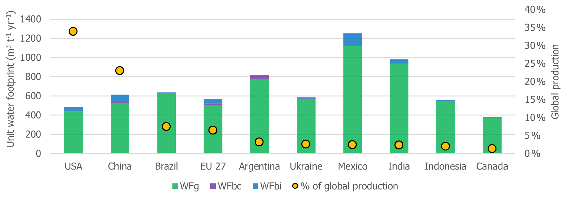
Figure 5Average unit water footprint of maize (g – green, bc – blue from capillary rise, bi – blue from irrigation) in cubic metres per tonne per year (m3 t−1 yr−1) and percentage of global production of the 10 biggest maize producers during 2012–2016.
3.2 Historical trends
The global average unit WF of maize has reduced over the last decades as shown in Fig. 6. When compared to 1986–1990, the average WF of 2012–2016 is 34.5 % smaller. However, not all unit WF components reduced by the same magnitude. WFg and WFbc reduced by nearly one-third between the two periods (−35.7 % and −31.0 %, respectively), while WFbi reduced by only 16.6 %. Therefore, the fraction of blue water in the average WF has increased by 23.9 % (+5.4 % for WFbc and +27.4 % for WFbi).
To explain the decreasing trend in the global average unit WF, the main contributing factors – Ys, CWU, and S (see Sect. 2.1.3) – are analysed with the Mann–Kendall trend test (Hussain and Mahmud, 2019). We detect significantly increasing trends in S (+51.5 % since 1986; ) and CWU (−0.37 % since 1986; ) and no significant trend in Ys (p=0.54). Subsequent correlation analysis shows that WF significantly correlates only with S (, ) and CWU (, ). Hence, the reduction in the WF can mainly be attributed to the increase in S, which reflects the historical agricultural advances (see Sect. 2.1.4). Once detrended, the WF only correlates significantly with Ys (; ), and thus the interannual variations in the WF are mainly driven by Ys response to climatic variability. For example, the WF peaks around 1988 and 2012 (see Fig. 6) are likely due to extreme La Niña-driven droughts in major maize-producing areas which caused substantial drops in crop yields (Iizumi et al., 2014; Rippey, 2015). A summary of global average annual WFs and main contributing factors during 1986–2016 is provided in Table S4.
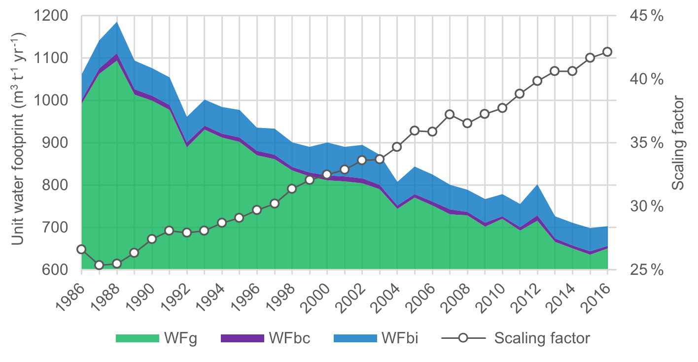
Figure 6Global trends in average unit water footprints (g – green, bc – blue from capillary rise, bi – blue from irrigation) in cubic metres per tonne per year (m3 t−1 yr−1) and yield scaling factors of maize from 1986 to 2016. Note that both y axes do not start at zero.
All major maize-producing areas show smaller average unit WFs in 2012–2016 compared to 1986–1990 (see Fig. 7). The regions with the largest WF reductions are Southern Africa (−60.3 %), Melanesia (−60.1 %), and South-eastern Asia (−59.1 %), which indicates substantial increases in maize yields. On the other hand, the regions with the smallest reductions are Western Europe (−20.5 %), Western Africa (−22.3 %), and Eastern Africa (−22.8 %). In the case of Western Europe, this is due to the already small WF in 1986–1990 (545.1 m3 t−1 yr−1), and thus there was a low potential for its reduction. In the case of Western and Eastern Africa, there was a high reduction potential, but it was barely realised, likely due to underlying socio-economic limitations (Smale et al., 2011).
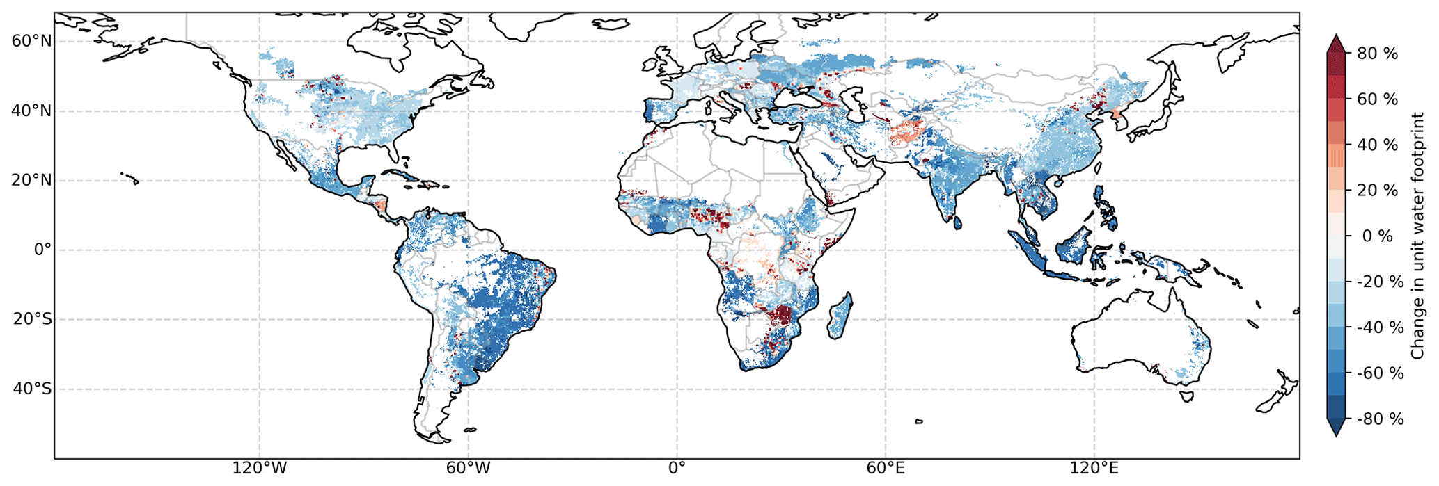
Figure 7Relative change in unit water footprint of maize from the average of 1986–1990 to the average of 2012–2016 at 5×5 arcmin resolution.
Among the countries that together account for 95 % of global maize production, reductions of more than 50 % are in Brazil, Indonesia, South Africa, the Philippines, Vietnam, Pakistan, and Paraguay (see Table S3). On the other hand, three countries that have increases in unit WFs (see Fig. 8) but together produce only 0.77 % of maize globally are the Democratic Republic of Congo (+9.7 %), Kenya (+12.7 %), and the Democratic People's Republic of Korea (+32.2 %). In the first two countries, this is due to an overall decreasing trend in maize yields and high interannual variability (see Sect. 3.3). Different dynamics can be observed in North Korea, where maize yields have dropped dramatically since the mid-1990s – the period known as the “North Korean famine” (Woo-Cumings, 2002). The yields have not yet recovered resulting in a larger unit WF.
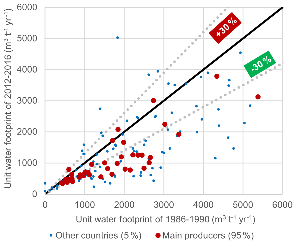
Figure 8Comparison of the national unit water footprints of maize (m3 t−1 yr−1) between the average of 1986–1990 and the average of 2012–2016. The black line represents no change, and the dotted grey lines show +30 % and −30 % changes.
The global WF of maize production has increased by 49.6 % since 1986 (see Fig. 9), peaking at 768.3×10⁹ m3 yr−1 in 2016. This increase differs among production systems. In rainfed systems, the consumption of green and blue water (from CR) has increased by 39.9 % and 67.0 %, respectively. In irrigated systems, it has increased by 108.4 % and 72.5 %, respectively. The Mann–Kendall trend test detects significantly increasing trends in the two main contributing factors: rainfed harvested area (+39.5 % since 1986; ) and irrigated harvested area (+107.2 % since 1986; ). Subsequent correlation analysis shows a significant correlation with both factors (r=0.98 each). Hence, the expansion of harvested areas increases global maize water consumption despite the reduction in unit WFs. The detrended global WF of production correlates significantly with the detrended harvested areas (rainfed r=0.95; irrigated r=0.86), which means that historical changes in the harvested areas are responsible for interannual variations in the global WF.
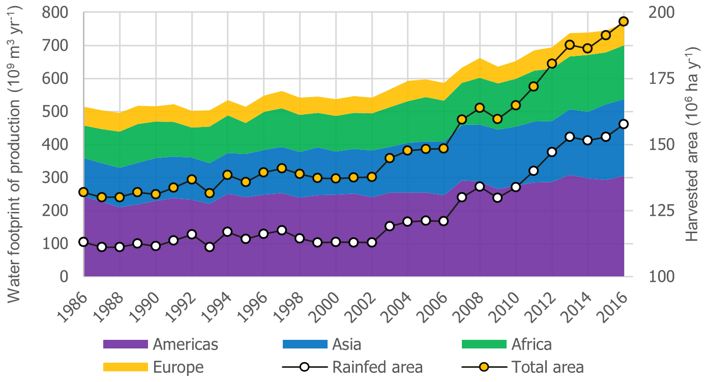
Figure 9Trends in the regional water footprints of production (109 m3 yr−1) and global harvested areas (106 ha yr−1) of maize from 1986 to 2016. Oceania is not shown due to its negligible contribution. Note that the right y axis does not start at zero.
Most of the harvested area expansion since 1986 has occurred in Asia and Africa (+81.7 % and +76.1 %, respectively), which has led to substantial increases in the WFs of maize production (+96.8 % and +67 %). At the same time, the Americas and Europe have also increased their WFs of production (+26.3 % and +20.8 %), but the harvested areas have expanded moderately (+25.7 % and +14.4 %). One of the main reasons behind a larger increase in WFs of production than in harvested areas lies in the expansion of irrigated systems. They have a larger CWU than rainfed systems (+17.3 % on average), and hence the regions with a larger expansion of irrigated systems, such as +204.7 % in Asia (compared to +45.0 % in rainfed systems), experience an increase in the average CWU. As a result, the share of irrigated maize in the global WF of production increased from 16.8 % in 1986 to 22.0 % in 2016. Besides the increase in feed demand, one of the main driving forces for maize area expansion is biofuel production. For example, nearly 40 % of maize in the USA is grown to produce bioethanol (Ranum et al., 2014).
3.3 Interannual variability
The interannual variability in detrended unit WFs of maize is analysed using the coefficient of variation (CV). The global average CV over the 1986–2016 period is 19.8 %. The variability in rainfed systems (average CV of 26.1 %) differs around the world depending on water availability. For instance, the average CV of regions with CR contribution is 16.8 %, while many arid parts of Sub-Saharan Africa that completely rely on rainfall have CV values higher than 70 % (see Fig. 10). As a result, some years may have extremely low yields, leading to unit WF peaks of more than 5000 m3 t−1 yr−1 (see Fig. 4a). On the other hand, the unit WF variability in irrigated systems (average CV of 8.2 %) is generally low in all regions as also suggested by previous studies (Kucharik and Ramankutty, 2005; Osborne and Wheeler, 2013). The interannual variability also depends on the level of agricultural development and socio-economic stability. For example, the average CV of the mostly rainfed maize in Western Europe is 8.8 %, while the average CV of the mostly irrigated maize in Central Asia is 18.8 %. The CV values of other regions are listed in Table 2.
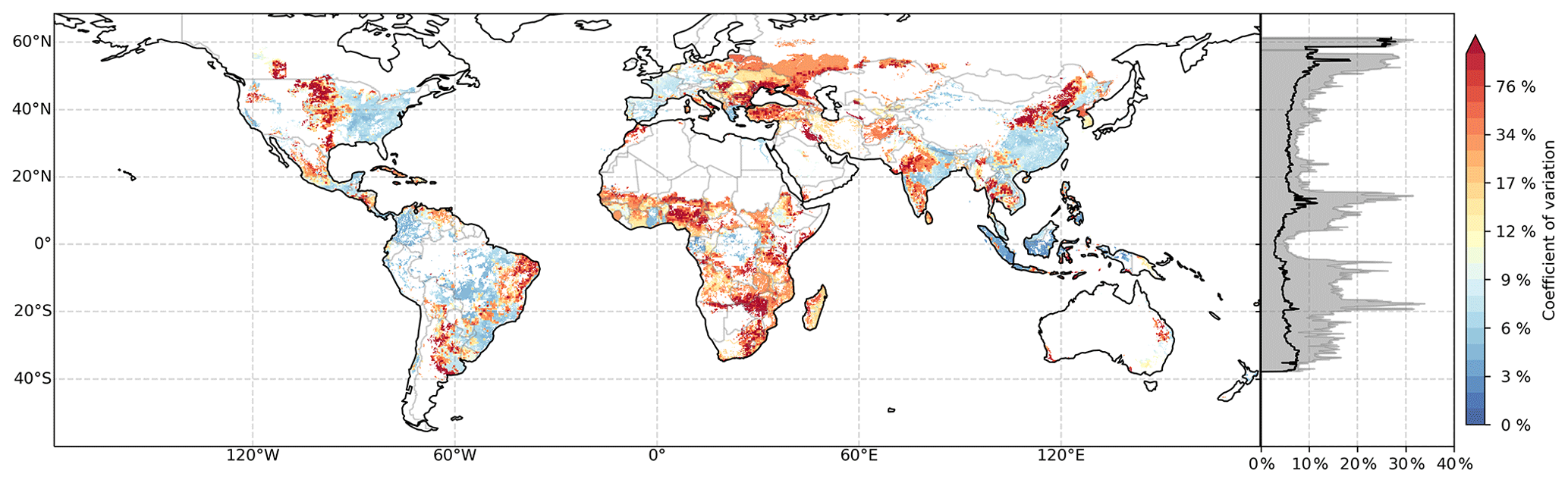
Figure 10Coefficient of variation of the detrended unit water footprints of maize during 1986–2016 at 5×5 arcmin resolution. The grey area in the side chart represents the median of all data points along the respective latitude, and the black line is the 10th percentile.
4.1 Comparison with literature
4.1.1 Average water footprints around 2000
Three previous studies have estimated maize WFs at the global scale with a distinction between green and blue water (see Table 3). All three focus on the period around year 2000. Therefore, we average our results over the 1996–2005 period to make the comparison. The previous studies agree with ours on the dominant role of green water. They also show larger global average unit WF estimates (ranging from +5 % to +23 %). Since the differences in the global average crop yields are relatively small (−4 % to +9 %), these larger WF estimates are likely caused by different methods of CWU estimation.
Table 3Comparison of ACEA results for maize with other global gridded studies. Numbers in brackets indicate the difference compared to the results of ACEA.

* Approximate estimates from the reported total water consumption as unit water footprint components were not explicitly provided.
Siebert and Döll (2010) estimate larger global average green and blue unit WFs compared to our study. The authors assume a predefined root depth and canopy development (in the initial, mid-, and late-season stages). In our study, both of them are driven by daily temperature and water availability, and thus the ability of maize to take up water and to transpire it can be limited by abiotic stresses (e.g. constrained root and canopy expansion, induced stomatal closure). Therefore, we likely simulate a smaller CWU compared to Siebert and Döll (2010). There are several other reasons for differences in CWU, but to what degree they explain the smaller estimates in ACEA is difficult to answer. Siebert and Döll (2010) consider a constant growing season duration using the crop calendar based on year 2000, while in our model the growing season duration is temperature-dependent, and the crop calendar is a composite of multiple recent data sources (see Sect. 2.1.4). Consequently, crop calendar days differ among the two studies, leading to different daily weather conditions and growing season durations. This results in different ET rates and hence different CWUs. Moreover, the authors estimate green and blue CWU with methods that are less precise than the daily green–blue accounting in ACEA (see Sect. 2.1.2). Siebert and Döll (2010) also cover a shorter historical period and use two older input datasets, i.e. climatic data that directly affect water availability and ET rates and harvested area data that affect the averaging of results.
Mekonnen and Hoekstra (2011) also show larger green and blue unit WFs. The authors use a similar modelling approach as Siebert and Döll (2010), but they simulate only 1 representative year, which neglects the interannual variability in climatic variables as well as trends in agricultural developments and harvested areas. Therefore, CWU estimates do not capture years with abnormal weather (wet, dry, cold, warm). Nevertheless, at the national level, both studies correlate well (r=0.95).
Tuninetti et al. (2015) report larger green but smaller blue unit WFs. The authors do not model the reference evapotranspiration and crop yields (as the other studies do) but take both from literature instead. Moreover, they equalise the blue CWU to irrigation supply which is calculated using independent data sources of different temporal and spatial resolutions.
The methodological differences among these three studies also lead to different estimates of the global WF of maize production. Compared to our study, Siebert and Döll (2010) and Mekonnen and Hoekstra (2011) report 16 %–18 % larger global WFs (15 %–17 % larger green and 8 %–53 % larger blue), while Tuninetti et al. (2015) report a half larger global WF (55 % larger green but 12 % smaller blue).
Table 4Comparison of crop water use (CWU) of rainfed and irrigated maize with field studies.

* According to FAO classification (Allen et al., 1998).
4.1.2 Other comparisons
The recent literature review of 70 related studies by Feng et al. (2021) reports the global average unit WF of maize of 730 m3 t−1 yr−1 (CV of 15.9 %) in 2002–2018. This aligns well with our estimate of 728.0 m3 t−1 yr−1 (CV of 19.8 %) in 2012–2016. Our estimates of maize CWU also align well with the literature. Jägermeyr et al. (2021a) simulate CWU for both rainfed and irrigated maize with multiple GGCMs at 30×30 arcmin resolution. The global medians are similar to ours, as can be observed in Fig. S3. Moreover, we compare our maize CWU estimates to several field studies in various years and locations (see Table 4). The differences between ACEA's values and the ones reported in literature vary between −9.4 % and +14.8 %. Irrigated maize shows smaller differences than rainfed maize for most of the considered studies. This may not be a model but rather a data accuracy issue. It is likely that the gridded meteorological data we use with a spatial resolution of 30×30 arcmin (see Sect. 2.2) deviate from measured data at the fields in the other studies. This is particularly relevant for rainfall, which shows strong spatial variability at small scales.
Approximate comparisons can also be done for maize yield gaps. Three studies estimate the global yield gaps around 2000 in a range of 50 %–64 % (Licker et al., 2010; Mueller et al., 2012; Neumann et al., 2010). Our estimate of the water-limited yield gap for 1996–2005 in ACEA is 67.3 %. Two more recent studies report yield gaps around 2010 for several locations in different regions (Hoffmann et al., 2018; Edreira et al., 2018). Their estimates show similarities to our study (calculated for 2012–2016): 80 % yield gap in Sub-Saharan Africa (77.5 % in ACEA), 20 % in Northern America (31.0 % in ACEA), and 38 % in East Asia (55.7 % in ACEA). The more pessimistic results of our study are likely due to differences in yield-limiting factors and harvested areas.
4.2 Strengths and weaknesses of ACEA
4.2.1 Advancing crop water productivity research
ACEA is a new GGCM that can estimate crop yield and CWU distinguishing three water types: green water, blue water from CR, and blue water from irrigation. The open-source nature and easy customisation in ACEA facilitate the analyses of crop water productivity responses to various environmental and managerial changes. Furthermore, the optimised modelling procedure allows for computationally efficient large-scale simulations. In our case, ACEA took 12 h to simulate 57 000 combinations of grid cells and setups (34 years long each; see Sect. 2.2) on a working station with 12 CPUs. This corresponds to 160 000 simulated years per computational hour. Compared to the reported performance of AquaCrop-GIS (Lorite et al., 2013), ACEA is up to 25 times faster. Simulation inputs for this study take more than 27.3 GB of space and outputs more than 30.2 GB.
4.2.2 Uncertainties in global crop modelling
Global gridded crop modelling is a complex process that contains many uncertainties (Folberth et al., 2019), and ACEA is not an exception. Most of the uncertainties likely originate from spatial and temporal resolutions of input datasets rather than from the model itself. We simulate maize production at 30×30 arcmin resolution, meaning that input datasets with finer resolutions have to be upscaled, such as soil characteristics and shallow groundwater levels (see Sect. 2.2). Then, we distribute the results among 5×5 arcmin grid cells according to the spatial distribution of harvested areas. This leads to uncertainty as the distributed results do not reflect the exact environmental conditions in each 5×5 arcmin grid cell. Alternatively, we could run ACEA at a finer resolution, but this was not feasible due to input data limitations and high computational requirements.
Next, selected crop parameters are based on a single maize cultivar from FAO (Hsiao et al., 2009). Therefore, the regional and historical differences in crop variety are not directly considered but incorporated in yield scaling factors (see Sect. 2.1.4). Moreover, the lack of subnational data needed to generate reliable crop calendars results in a rough representation of spatial variability in planting and harvest dates. Thus, the start and duration of growing seasons might be miscalculated. As the current version of ACEA does not consider chemical cycles between a crop and the environment, the biophysical stresses from water salinity and insufficient nutrient intake are not simulated, which again leads to uncertainties in our results.
We also assume the same soil-moisture-based rule for irrigation application in all grid cells. In reality, farmers decide when and how much to irrigate based on site-specific conditions such as access to water and technological inputs. Furthermore, the water consumed by irrigation conveyance is not accounted for. Therefore, the timing and volume of irrigation events simulated in ACEA can deviate from the actual ones. As for CR, we consider neither interannual variations in groundwater levels nor the effects of pumping, and thus our WFbc estimates rather reflect potential values under steady-state conditions.
Finally, the post-processing of results also contains uncertainties. In particular, the distribution of extrapolated harvested areas (see Sect. 2.2) plays an important role during spatial averaging. The resulted uncertainties are particularly relevant when zooming to smaller geographical scales (e.g. analysis of small countries).
4.3 Sustainability of maize production
Global maize production has soared in recent decades due to high demands from livestock and biofuel industries. For example, in the USA, these industries consume almost 90 % of all domestically produced maize (Ranum et al., 2014), and thus only a small fraction ends up on humans' plates. This does not only lead to debates of “food versus fuel” and “food versus feed” but also raises the question of the environmental impacts of maize production (Wallington et al., 2012). Although assessing the latter is out of the scope of our study, we highlight several sustainability aspects of maize production that could be addressed in further research. Concerning water resources, there are three key aspects:
-
To what extent WFs of maize production contribute to local green (Schyns et al., 2019) and blue water scarcity (Mekonnen and Hoekstra, 2016). For example, the WFs of production can be compared to local time-specific environmental limits of water consumption (Hogeboom et al., 2020; Mekonnen and Hoekstra, 2020).
-
How local unit WFs of maize compare to appropriate benchmarks. These benchmarks refer to unit WFs that are either obtained by the best producers in other areas with similar agro-environmental conditions or can be achieved using best available practices (Mekonnen and Hoekstra, 2014). Examples of such practices are the application of mulches, selection of better crop varieties, and optimisation of irrigation and nutrient supply (Chukalla et al., 2015; Rusinamhodzi et al., 2012).
-
To what extent maize production pollutes the local water resources via applied fertilisers, herbicides, and pesticides. This pollution can be quantified by water quality indicators, such as the grey WF (Chukalla et al., 2018a; Mekonnen and Hoekstra, 2010; Liu et al., 2017), which refers to the volume of water needed to assimilate a load of pollutants to freshwater bodies. This load can be minimised with agroecological practices, such as the application of organic alternatives to agrochemicals and intercropping (or crop rotation) with nitrogen-fixing plants (e.g. alfalfa, soybeans) (Capellesso et al., 2016). In this context, it is also worthwhile to study the trade-offs between the consumptive (green plus blue) and grey WFs, as the alternative agroecological practices also affect the former (Chukalla et al., 2018b).
The sustainability of maize production can also be assessed from other perspectives than water, e.g. by addressing questions around impacts on ecosystems (Fletcher et al., 2011; Immerzeel et al., 2014), associated GHG emissions (Yang and Chen, 2013; Dias De Oliveira et al., 2005), equitable crop markets (Marenya et al., 2017; Mmbando et al., 2015), and economic value (Wallington et al., 2012; Baffes et al., 2019).
ACEA is a new process-based crop model that allows for the assessment of green and blue crop water productivity at large spatial scales, which we demonstrate by simulating global maize WFs over the 1986–2016 period. Our results show that the current global average unit WF of maize is 728.0 m3 t−1 yr−1. The WF composition is dominated by green water, but the share of blue water from irrigation is increasing. The share of blue water from CR is minor at the global scale but can be substantial in areas with the presence of shallow groundwater. Unit WFs vary greatly around the world. Regions characterised by high-input agriculture generally have a small unit WF and corresponding CV, such as Western Europe and Northern America (WF<500 m3 t−1 yr−1, CV<17 %). Conversely, low-input regions show opposite outcomes, such as in Middle and Eastern Africa (WF>2500 m3 t−1 yr−1, CV>30 %). Nevertheless, we observe unit WF reductions in most regions due to the historical increase in maize yields. As a result, the global average unit WF has reduced by 34.5 % since 1986. Despite this productivity gain, the global WF of maize production has increased by 49.6 % due to the expansion of rainfed and irrigated areas. Both trends are likely to continue as the yield gaps are closing and maize areas are further expanding driven by demands from food, livestock, and biofuel industries. Therefore, it is important to address the sustainability and purpose of maize production as it might endanger local ecosystems and human livelihoods, e.g. by polluting water resources and contributing to water scarcity.
Input and output datasets that are not provided in the paper or the Supplement as well as Python scripts may be provided by the corresponding author upon request.
The supplement related to this article is available online at: https://doi.org/10.5194/hess-26-923-2022-supplement.
OM, JFS, and MJB designed the study and the model. OM wrote the code and carried out the simulations. With contributions from all co-authors, OM did the analysis and prepared the manuscript.
The contact author has declared that neither they nor their co-authors have any competing interests.
Publisher's note: Copernicus Publications remains neutral with regard to jurisdictional claims in published maps and institutional affiliations.
We dedicate our study to Arjen Y. Hoekstra (1967–2019), who initiated this research but unfortunately passed away before it was published. The ACEA simulations were partly carried out using the Dutch national e-infrastructure with the support of SURF Cooperative.
This research has been supported by the H2020 European Research Council (EARTH@LTERNATIVES (grant no. 834716)).
This paper was edited by Giuliano Di Baldassarre and reviewed by three anonymous referees.
Abraha, M., Chen, J., Hamilton, S. K., and Robertson, G. P.: Long-term evapotranspiration rates for rainfed corn versus perennial bioenergy crops in a mesic landscape, Hydrol. Process., 34, 810–822, https://doi.org/10.1002/hyp.13630, 2020.
Allen, R. G., Pereira, L. S., Raes, D., and Smith, M.: Crop evapotranspiration: guidelines for computing crop water requirements, FAO irrigation and drainage paper 56, Food and Agriculture Organization of the United Nations, Rome, 300 pp., ISBN 92-5-104219-5, https://www.fao.org/3/X0490E/x0490e00.htm (last access: 14 February 2022)1998.
Amante, C.: ETOPO1 1 Arc-Minute Global Relief Model: Procedures, Data Sources and Analysis, NOAA, https://doi.org/10.7289/V5C8276M, 2009.
Andarzian, B., Bannayan, M., Steduto, P., Mazraeh, H., Barati, M. E., Barati, M. A., and Rahnama, A.: Validation and testing of the AquaCrop model under full and deficit irrigated wheat production in Iran, Agricult. Water Manage., 100, 1–8, https://doi.org/10.1016/j.agwat.2011.08.023, 2011.
Araya, A., Kisekka, I., and Holman, J.: Evaluating deficit irrigation management strategies for grain sorghum using AquaCrop, Irrig. Sci., 34, 465–481, https://doi.org/10.1007/s00271-016-0515-7, 2016.
Baffes, J., Kshirsagar, V., and Mitchell, D.: What Drives Local Food Prices? Evidence from the Tanzanian Maize Market, The World Bank Economic Review, 33, 160–184, https://doi.org/10.1093/wber/lhx008, 2019.
Brown, C. E.: Applied multivariate statistics in geohydrology and related sciences, Springer, Berlin, New York, ISBN 978-3-642-80328-4, 1998.
Campbell, B. M., Beare, D. J., Bennett, E. M., Hall-Spencer, J. M., Ingram, J. S. I., Jaramillo, F., Ortiz, R., Ramankutty, N., Sayer, J. A., and Shindell, D.: Agriculture production as a major driver of the Earth system exceeding planetary boundaries, Ecol. Soc., 22, 8, https://doi.org/10.5751/ES-09595-220408, 2017.
Capellesso, A. J., Cazella, A. A., Schmitt Filho, A. L., Farley, J., and Martins, D. A.: Economic and environmental impacts of production intensification in agriculture: comparing transgenic, conventional, and agroecological maize crops, Agroecol. Sustain. Food Syst., 40, 215–236, https://doi.org/10.1080/21683565.2015.1128508, 2016.
Chapagain, A. K. and Hoekstra, A. Y.: The blue, green and grey water footprint of rice from production and consumption perspectives, Ecol. Econ., 70, 749–758, https://doi.org/10.1016/j.ecolecon.2010.11.012, 2011.
Chukalla, A. D., Krol, M. S., and Hoekstra, A. Y.: Green and blue water footprint reduction in irrigated agriculture: effect of irrigation techniques, irrigation strategies and mulching, Hydrol. Earth Syst. Sci., 19, 4877–4891, https://doi.org/10.5194/hess-19-4877-2015, 2015.
Chukalla, A. D., Krol, M. S., and Hoekstra, A. Y.: Grey water footprint reduction in irrigated crop production: effect of nitrogen application rate, nitrogen form, tillage practice and irrigation strategy, Hydrol. Earth Syst. Sci., 22, 3245–3259, https://doi.org/10.5194/hess-22-3245-2018, 2018a.
Chukalla, A. D., Krol, M. S., and Hoekstra, A. Y.: Trade-off between blue and grey water footprint of crop production at different nitrogen application rates under various field management practices, Sci. Total Environ., 626, 962–970, https://doi.org/10.1016/j.scitotenv.2018.01.164, 2018b.
DeJonge, K. C., Ascough, J. C., Andales, A. A., Hansen, N. C., Garcia, L. A., and Arabi, M.: Improving evapotranspiration simulations in the CERES-Maize model under limited irrigation, Agricult. Water Manage., 115, 92–103, https://doi.org/10.1016/j.agwat.2012.08.013, 2012.
Deryng, D., Elliott, J., Folberth, C., Müller, C., Pugh, T. A. M., Boote, K. J., Conway, D., Ruane, A. C., Gerten, D., Jones, J. W., Khabarov, N., Olin, S., Schaphoff, S., Schmid, E., Yang, H., and Rosenzweig, C.: Regional disparities in the beneficial effects of rising CO2 concentrations on crop water productivity, Nat. Clim. Change, 6, 786–790, https://doi.org/10.1038/nclimate2995, 2016.
Dias De Oliveira, M. E., Vaughan, B. E., and Rykiel, E. J.: Ethanol as Fuel: Energy, Carbon Dioxide Balances, and Ecological Footprint, BioScience, 55, 593, https://doi.org/10.1641/0006-3568(2005)055[0593:EAFECD]2.0.CO;2, 2005.
Djaman, K., O'Neill, M., Owen, C., Smeal, D., Koudahe, K., West, M., Allen, S., Lombard, K., and Irmak, S.: Crop Evapotranspiration, Irrigation Water Requirement and Water Productivity of Maize from Meteorological Data under Semiarid Climate, Water, 10, 405, https://doi.org/10.3390/w10040405, 2018.
Dlugokencky, E. and Tans, P.: Trends in Atmospheric Carbon Dioxide, https://www.esrl.noaa.gov/gmd/ccgg/trends/gl_data.html, last access: 14 September 2020.
Duvick, D. N.: The Contribution of Breeding to Yield Advances in maize (Zea mays L.), in: Advances in Agronomy, vol. 86, Elsevier, 83–145, https://doi.org/10.1016/S0065-2113(05)86002-X, 2005.
Edreira, J. I. R., Guilpart, N., Sadras, V., Cassman, K. G., van Ittersum, M. K., Schils, R. L. M., and Grassini, P.: Water productivity of rainfed maize and wheat: A local to global perspective, Agr. Forest Meteorol., 259, 364–373, https://doi.org/10.1016/j.agrformet.2018.05.019, 2018.
Elliott, J., Müller, C., Deryng, D., Chryssanthacopoulos, J., Boote, K. J., Büchner, M., Foster, I., Glotter, M., Heinke, J., Iizumi, T., Izaurralde, R. C., Mueller, N. D., Ray, D. K., Rosenzweig, C., Ruane, A. C., and Sheffield, J.: The Global Gridded Crop Model Intercomparison: data and modeling protocols for Phase 1 (v1.0), Geosci. Model Dev., 8, 261–277, https://doi.org/10.5194/gmd-8-261-2015, 2015.
Fader, M., Rost, S., Müller, C., Bondeau, A., and Gerten, D.: Virtual water content of temperate cereals and maize: Present and potential future patterns, J. Hydrol., 384, 218–231, https://doi.org/10.1016/j.jhydrol.2009.12.011, 2010.
Fan, Y., Li, H., and Miguez-Macho, G.: Global Patterns of Groundwater Table Depth, Science, 339, 940–943, https://doi.org/10.1126/science.1229881, 2013.
FAOSTAT: Food and agriculture data, http://www.fao.org/faostat, last access: 15 May 2021.
Feng, B., Zhuo, L., Xie, D., Mao, Y., Gao, J., Xie, P., and Wu, P.: A quantitative review of water footprint accounting and simulation for crop production based on publications during 2002–2018, Ecol. Indicat., 120, 106962, https://doi.org/10.1016/j.ecolind.2020.106962, 2021.
Fletcher, R. J., Robertson, B. A., Evans, J., Doran, P. J., Alavalapati, J. R., and Schemske, D. W.: Biodiversity conservation in the era of biofuels: risks and opportunities, Front. Ecol. Environ., 9, 161–168, https://doi.org/10.1890/090091, 2011.
Folberth, C., Elliott, J., Müller, C., Balkovič, J., Chryssanthacopoulos, J., Izaurralde, R. C., Jones, C. D., Khabarov, N., Liu, W., Reddy, A., Schmid, E., Skalský, R., Yang, H., Arneth, A., Ciais, P., Deryng, D., Lawrence, P. J., Olin, S., Pugh, T. A. M., Ruane, A. C., and Wang, X.: Parameterization-induced uncertainties and impacts of crop management harmonization in a global gridded crop model ensemble, PLoS ONE, 14, e0221862, https://doi.org/10.1371/journal.pone.0221862, 2019.
Franke, J. A., Müller, C., Elliott, J., Ruane, A. C., Jägermeyr, J., Snyder, A., Dury, M., Falloon, P. D., Folberth, C., François, L., Hank, T., Izaurralde, R. C., Jacquemin, I., Jones, C., Li, M., Liu, W., Olin, S., Phillips, M., Pugh, T. A. M., Reddy, A., Williams, K., Wang, Z., Zabel, F., and Moyer, E. J.: The GGCMI Phase 2 emulators: global gridded crop model responses to changes in CO2, temperature, water, and nitrogen (version 1.0), Geosci. Model Dev., 13, 3995–4018, https://doi.org/10.5194/gmd-13-3995-2020, 2020.
Gardiol, J. M., Serio, L. A., and Della Maggiora, A. I.: Modelling evapotranspiration of corn (Zea mays) under different plant densities, J. Hydrol., 271, 188–196, https://doi.org/10.1016/S0022-1694(02)00347-5, 2003.
Giordano, M. A., Rijsberman, F. R., Saleth, R. M., and International Water Management Institute (Eds.): More crop per drop: revisiting a research paradigm: results and synthesis of IWMI's research, 1996–2005, IWA Pub, London, UK, 273 pp., ISBN 978-1-84339-112-8, 2006.
Greaves, G. and Wang, Y.-M.: Assessment of FAO AquaCrop Model for Simulating Maize Growth and Productivity under Deficit Irrigation in a Tropical Environment, Water, 8, 557, https://doi.org/10.3390/w8120557, 2016.
Greve, P., Kahil, T., Mochizuki, J., Schinko, T., Satoh, Y., Burek, P., Fischer, G., Tramberend, S., Burtscher, R., Langan, S., and Wada, Y.: Global assessment of water challenges under uncertainty in water scarcity projections, Nat. Sustain., 1, 486–494, https://doi.org/10.1038/s41893-018-0134-9, 2018.
Grosso, C., Manoli, G., Martello, M., Chemin, Y., Pons, D., Teatini, P., Piccoli, I., and Morari, F.: Mapping Maize Evapotranspiration at Field Scale Using SEBAL: A Comparison with the FAO Method and Soil-Plant Model Simulations, Remote Sens., 10, 1452, https://doi.org/10.3390/rs10091452, 2018.
Han, C., Zhang, B., Chen, H., Liu, Y., and Wei, Z.: Novel approach of upscaling the FAO AquaCrop model into regional scale by using distributed crop parameters derived from remote sensing data, Agricult. Water Manage., 240, 106288, https://doi.org/10.1016/j.agwat.2020.106288, 2020.
Hoekstra, A. Y. (Ed.): The water footprint assessment manual: setting the global standard, Earthscan, London, Washington, DC, 203 pp., ISBN 978-1-84971-279-8, 2011.
Hoekstra, A. Y.: Green-blue water accounting in a soil water balance, Adv. Water Resour., 129, 112–117, https://doi.org/10.1016/j.advwatres.2019.05.012, 2019.
Hoekstra, A. Y. and Mekonnen, M. M.: The water footprint of humanity, P. Natl. Acad. Sci. USA, 109, 3232–3237, https://doi.org/10.1073/pnas.1109936109, 2012.
Hoekstra, A. Y., Booij, M. J., Hunink, J. C., and Meijer, K. S.: Blue water footprint of agriculture, industry, households and water management in the Netherlands: An exploration of using the Netherlands Hydrological Instrument, Unesco – IHE Institute for Water Education, Delft, the Netherlands, https://doi.org/10.13140/RG.2.1.2276.3043, 2012a.
Hoekstra, A. Y., Mekonnen, M. M., Chapagain, A. K., Mathews, R. E., and Richter, B. D.: Global Monthly Water Scarcity: Blue Water Footprints versus Blue Water Availability, PLoS ONE, 7, e32688, https://doi.org/10.1371/journal.pone.0032688, 2012b.
Hoffmann, M. P., Haakana, M., Asseng, S., Höhn, J. G., Palosuo, T., Ruiz-Ramos, M., Fronzek, S., Ewert, F., Gaiser, T., Kassie, B. T., Paff, K., Rezaei, E. E., Rodríguez, A., Semenov, M., Srivastava, A. K., Stratonovitch, P., Tao, F., Chen, Y., and Rötter, R. P.: How does inter-annual variability of attainable yield affect the magnitude of yield gaps for wheat and maize? An analysis at ten sites, Agricult. Syst., 159, 199–208, https://doi.org/10.1016/j.agsy.2017.03.012, 2018.
Hogeboom, R. J., Bruin, D., Schyns, J. F., Krol, M. S., and Hoekstra, A. Y.: Capping Human Water Footprints in the World's River Basins, Earth's Future, 8, e2019EF001363, https://doi.org/10.1029/2019EF001363, 2020.
Hsiao, T. C., Heng, L., Steduto, P., Rojas-Lara, B., Raes, D., and Fereres, E.: AquaCrop-The FAO Crop Model to Simulate Yield Response to Water: III. Parameterization and Testing for Maize, Agron. J., 101, 448–459, https://doi.org/10.2134/agronj2008.0218s, 2009.
Huang, J., Scherer, L., Lan, K., Chen, F., and Thorp, K. R.: Advancing the application of a model-independent open-source geospatial tool for national-scale spatiotemporal simulations, Environ. Model. Softw., 119, 374–378, https://doi.org/10.1016/j.envsoft.2019.07.003, 2019.
Hussain, Md. and Mahmud, I.: pyMannKendall: a python package for non parametric Mann Kendall family of trend tests, J. Open Source Softw., 4, 1556, https://doi.org/10.21105/joss.01556, 2019.
Iizumi, T., Luo, J.-J., Challinor, A. J., Sakurai, G., Yokozawa, M., Sakuma, H., Brown, M. E., and Yamagata, T.: Impacts of El Niño Southern Oscillation on the global yields of major crops, Nat. Commun., 5, 3712, https://doi.org/10.1038/ncomms4712, 2014.
Immerzeel, D. J., Verweij, P. A., van der Hilst, F., and Faaij, A. P. C.: Biodiversity impacts of bioenergy crop production: a state-of-the-art review, GCB Bioenergy, 6, 183–209, https://doi.org/10.1111/gcbb.12067, 2014.
Irmak, S. and Djaman, K.: Effects of Planting Date and Density on Plant Growth, Yield, Evapotranspiration, and Water Productivity of Subsurface Drip-Irrigated and Rainfed Maize, T. ASABE, 59, 1235–1256, https://doi.org/10.13031/trans.59.11169, 2016.
ISIMIP: ISIMIP3 simulation protocol, https://protocol.isimip.org/protocol/ISIMIP3b/agriculture.html, last access: 14 September 2020.
Jägermeyr, J., Gerten, D., Heinke, J., Schaphoff, S., Kummu, M., and Lucht, W.: Water savings potentials of irrigation systems: global simulation of processes and linkages, Hydrol. Earth Syst. Sci., 19, 3073–3091, https://doi.org/10.5194/hess-19-3073-2015, 2015.
Jägermeyr, J., Müller, C., Ruane, A. C., Elliott, J., Balkovic, J., Castillo, O., Faye, B., Foster, I., Folberth, C., Franke, J. A., Fuchs, K., Guarin, J. R., Heinke, J., Hoogenboom, G., Iizumi, T., Jain, A. K., Kelly, D., Khabarov, N., Lange, S., Lin, T.-S., Liu, W., Mialyk, O., Minoli, S., Moyer, E. J., Okada, M., Phillips, M., Porter, C., Rabin, S. S., Scheer, C., Schneider, J. M., Schyns, J. F., Skalsky, R., Smerald, A., Stella, T., Stephens, H., Webber, H., Zabel, F., and Rosenzweig, C.: Climate impacts on global agriculture emerge earlier in new generation of climate and crop models, Nat. Food, 2, 873–885, https://doi.org/10.1038/s43016-021-00400-y, 2021a.
Jägermeyr, J., Müller, C., Minoli, S., Ray, D., and Siebert, S.: GGCMI Phase 3 crop calendar, Zenodo [data set], https://doi.org/10.5281/ZENODO.5062513, 2021b.
Jaramillo, F. and Destouni, G.: Local flow regulation and irrigation raise global human water consumption and footprint, Science, 350, 1248–1251, https://doi.org/10.1126/science.aad1010, 2015.
Karandish, F. and Hoekstra, A.: Informing National Food and Water Security Policy through Water Footprint Assessment: the Case of Iran, Water, 9, 831, https://doi.org/10.3390/w9110831, 2017.
Kelly, T. D. and Foster, T.: AquaCrop-OSPy: Bridging the gap between research and practice in crop-water modeling, Agricult. Water Manage., 254, 106976, https://doi.org/10.1016/j.agwat.2021.106976, 2021.
Khoshravesh, M., Mostafazadeh-Fard, B., Heidarpour, M., and Kiani, A.-R.: AquaCrop model simulation under different irrigation water and nitrogen strategies, Water Sci. Technol., 67, 232–238, https://doi.org/10.2166/wst.2012.564, 2013.
Klein Goldewijk, K., Beusen, A., Doelman, J., and Stehfest, E.: Anthropogenic land use estimates for the Holocene – HYDE 3.2, Earth Syst. Sci. Data, 9, 927–953, https://doi.org/10.5194/essd-9-927-2017, 2017.
Kucharik, C. J. and Ramankutty, N.: Trends and Variability in U.S. Corn Yields Over the Twentieth Century, Earth Interact., 9, 1–29, https://doi.org/10.1175/EI098.1, 2005.
Lange, S.: WFDE5 over land merged with ERA5 over the ocean (W5E5 v1.0) (1.0), Potsdam Institute for Climate Impact Research, https://doi.org/10.5880/PIK.2019.023, 2019.
Licker, R., Johnston, M., Foley, J. A., Barford, C., Kucharik, C. J., Monfreda, C., and Ramankutty, N.: Mind the gap: how do climate and agricultural management explain the `yield gap' of croplands around the world: Investigating drivers of global crop yield patterns, Global Ecol. Biogeogr., 19, 769–782, https://doi.org/10.1111/j.1466-8238.2010.00563.x, 2010.
Liu, J., Zehnder, A. J. B., and Yang, H.: Global consumptive water use for crop production: The importance of green water and virtual water: Global Consumptive Water Use, Water Resour. Res., 45, W05428, https://doi.org/10.1029/2007WR006051, 2009.
Liu, W., Yang, H., Folberth, C., Wang, X., Luo, Q., and Schulin, R.: Global investigation of impacts of PET methods on simulating crop-water relations for maize, Agr. Forest Meteorol., 221, 164–175, https://doi.org/10.1016/j.agrformet.2016.02.017, 2016.
Liu, W., Antonelli, M., Liu, X., and Yang, H.: Towards improvement of grey water footprint assessment: With an illustration for global maize cultivation, J. Clean. Product., 147, 1–9, https://doi.org/10.1016/j.jclepro.2017.01.072, 2017.
Lorenz, A. J., Gustafson, T. J., Coors, J. G., and de Leon, N.: Breeding Maize for a Bioeconomy: A Literature Survey Examining Harvest Index and Stover Yield and Their Relationship to Grain Yield, Crop Sci., 50, 1–12, https://doi.org/10.2135/cropsci2009.02.0086, 2010.
Lorite, I. J., García-Vila, M., Santos, C., Ruiz-Ramos, M., and Fereres, E.: AquaData and AquaGIS: Two computer utilities for temporal and spatial simulations of water-limited yield with AquaCrop, Comput. Electron. Agricult., 96, 227–237, https://doi.org/10.1016/j.compag.2013.05.010, 2013.
Lovarelli, D., Bacenetti, J., and Fiala, M.: Water Footprint of crop productions: A review, Sci. Total Environ., 548, 236–251, https://doi.org/10.1016/j.scitotenv.2016.01.022, 2016.
Maniruzzaman, M., Talukder, M. S. U., Khan, M. H., Biswas, J. C., and Nemes, A.: Validation of the AquaCrop model for irrigated rice production under varied water regimes in Bangladesh, Agricult. Water Manage., 159, 331–340, https://doi.org/10.1016/j.agwat.2015.06.022, 2015.
Marenya, P. P., Kassie, M. B., Jaleta, M. D., and Rahut, D. B.: Maize Market Participation among Female- and Male-Headed Households in Ethiopia, J. Develop. Stud., 53, 481–494, https://doi.org/10.1080/00220388.2016.1171849, 2017.
Mekonnen, M. M. and Hoekstra, A. Y.: A global and high-resolution assessment of the green, blue and grey water footprint of wheat, Hydrol. Earth Syst. Sci., 14, 1259–1276, https://doi.org/10.5194/hess-14-1259-2010, 2010.
Mekonnen, M. M. and Hoekstra, A. Y.: The green, blue and grey water footprint of crops and derived crop products, Hydrol. Earth Syst. Sci., 15, 1577–1600, https://doi.org/10.5194/hess-15-1577-2011, 2011.
Mekonnen, M. M. and Hoekstra, A. Y.: Water footprint benchmarks for crop production: A first global assessment, Ecol. Indicat., 46, 214–223, https://doi.org/10.1016/j.ecolind.2014.06.013, 2014.
Mekonnen, M. M. and Hoekstra, A. Y.: Four billion people facing severe water scarcity, Sci. Adv., 2, e1500323, https://doi.org/10.1126/sciadv.1500323, 2016.
Mekonnen, M. M. and Hoekstra, A. Y.: Sustainability of the blue water footprint of crops, Adv. Water Resour., 143, 103679, https://doi.org/10.1016/j.advwatres.2020.103679, 2020.
Minoli, S., Müller, C., Elliott, J., Ruane, A. C., Jägermeyr, J., Zabel, F., Dury, M., Folberth, C., François, L., Hank, T., Jacquemin, I., Liu, W., Olin, S., and Pugh, T. A. M.: Global Response Patterns of Major Rainfed Crops to Adaptation by Maintaining Current Growing Periods and Irrigation, Earth's Future, 7, 1464–1480, https://doi.org/10.1029/2018EF001130, 2019.
Mmbando, F. E., Wale, E. Z., and Baiyegunhi, L. J. S.: Welfare impacts of smallholder farmers' participation in maize and pigeonpea markets in Tanzania, Food Sec., 7, 1211–1224, https://doi.org/10.1007/s12571-015-0519-9, 2015.
Mueller, N. D., Gerber, J. S., Johnston, M., Ray, D. K., Ramankutty, N., and Foley, J. A.: Closing yield gaps through nutrient and water management, Nature, 490, 254–257, https://doi.org/10.1038/nature11420, 2012.
Müller, C., Elliott, J., Chryssanthacopoulos, J., Arneth, A., Balkovic, J., Ciais, P., Deryng, D., Folberth, C., Glotter, M., Hoek, S., Iizumi, T., Izaurralde, R. C., Jones, C., Khabarov, N., Lawrence, P., Liu, W., Olin, S., Pugh, T. A. M., Ray, D. K., Reddy, A., Rosenzweig, C., Ruane, A. C., Sakurai, G., Schmid, E., Skalsky, R., Song, C. X., Wang, X., de Wit, A., and Yang, H.: Global gridded crop model evaluation: benchmarking, skills, deficiencies and implications, Geosci. Model Dev., 10, 1403–1422, https://doi.org/10.5194/gmd-10-1403-2017, 2017.
Nachtergaele, F. O., van Velthuizen, H., Verelst, L., Batjes, N. H., Dijkshoorn, J. A., van Engelen, V. W. P., Fischer, G., Jones, A., Montanarella, L., Petri, M., Prieler, S., Teixeira, E., Wilberg, D., and Shi, X.: Harmonized World Soil Database (version 1.0), http://www.fao.org/fileadmin/templates/nr/documents/HWSD/HWSD_Documentation.pdf (last access: 14 February 2022), 2008.
Nagore, M. L., Echarte, L., Andrade, F. H., and Della Maggiora, A.: Crop evapotranspiration in Argentinean maize hybrids released in different decades, Field Crops Res., 155, 23–29, https://doi.org/10.1016/j.fcr.2013.09.026, 2014.
Neumann, K., Verburg, P. H., Stehfest, E., and Müller, C.: The yield gap of global grain production: A spatial analysis, Agricult. Syst., 103, 316–326, https://doi.org/10.1016/j.agsy.2010.02.004, 2010.
Osborne, T. M. and Wheeler, T. R.: Evidence for a climate signal in trends of global crop yield variability over the past 50 years, Environ. Res. Lett., 8, 024001, https://doi.org/10.1088/1748-9326/8/2/024001, 2013.
Portmann, F. T., Siebert, S., and Döll, P.: MIRCA2000-Global monthly irrigated and rainfed crop areas around the year 2000: A new high-resolution data set for agricultural and hydrological modeling: Monthly Irrigated And Rainfed Crop Areas, Global Biogeochem. Cy., 24, GB1011, https://doi.org/10.1029/2008GB003435, 2010.
QGIS: A Free and Open Source Geographic Information System, https://qgis.org/en/site/, last access: 16 June 2021.
Raes, D., Steduto, P., Hsiao, T. C., and Fereres, E.: AquaCrop-The FAO Crop Model to Simulate Yield Response to Water: II. Main Algorithms and Software Description, Agron. J., 101, 438–447, https://doi.org/10.2134/agronj2008.0140s, 2009.
Raes, D., Steduto, P., Hsiao, T. C., and Fereres, E.: AquaCrop Version 6.0 – 6.1: Reference manual (Annexes), Rome, https://www.fao.org/documents/card/en/c/BR244E (last access: 14 February 2022), 2018.
Ranum, P., Peña-Rosas, J. P., and Garcia-Casal, M. N.: Global maize production, utilization, and consumption, Ann. N.Y. Acad. Sci., 1312, 105–112, https://doi.org/10.1111/nyas.12396, 2014.
Rippey, B. R.: The U.S. drought of 2012, Weather Clim. Extrem., 10, 57–64, https://doi.org/10.1016/j.wace.2015.10.004, 2015.
Rosenzweig, C., Jones, J. W., Hatfield, J. L., Ruane, A. C., Boote, K. J., Thorburn, P., Antle, J. M., Nelson, G. C., Porter, C., Janssen, S., Asseng, S., Basso, B., Ewert, F., Wallach, D., Baigorria, G., and Winter, J. M.: The Agricultural Model Intercomparison and Improvement Project (AgMIP): Protocols and pilot studies, Agr. Forest Meteorol., 170, 166–182, https://doi.org/10.1016/j.agrformet.2012.09.011, 2013.
Ruane, A., Antle, J., Elliott, J., Folberth, C., Hoogenboom, G., Mason-D'Croz, D., Müller, C., Porter, C., Phillips, M., Raymundo, R., Sands, R., Valdivia, R., White, J., Wiebe, K., and Rosenzweig, C.: Biophysical and economic implications for agriculture of +1.5∘ and +2.0 ∘C global warming using AgMIP Coordinated Global and Regional Assessments, Clim. Res., 76, 17–39, https://doi.org/10.3354/cr01520, 2018.
Rudnick, D. R., Irmak, S., Djaman, K., and Sharma, V.: Impact of irrigation and nitrogen fertilizer rate on soil water trends and maize evapotranspiration during the vegetative and reproductive periods, Agr. Water Manage., 191, 77–84, https://doi.org/10.1016/j.agwat.2017.06.007, 2017.
Rusinamhodzi, L., Corbeels, M., Nyamangara, J., and Giller, K. E.: Maize–grain legume intercropping is an attractive option for ecological intensification that reduces climatic risk for smallholder farmers in central Mozambique, Field Crops Res., 136, 12–22, https://doi.org/10.1016/j.fcr.2012.07.014, 2012.
Saxton, K. E. and Rawls, W. J.: Soil Water Characteristic Estimates by Texture and Organic Matter for Hydrologic Solutions, Soil Sci. Soc. Am. J., 70, 1569–1578, https://doi.org/10.2136/sssaj2005.0117, 2006.
Schyns, J. F., Hoekstra, A. Y., Booij, M. J., Hogeboom, R. J., and Mekonnen, M. M.: Limits to the world's green water resources for food, feed, fiber, timber, and bioenergy, P. Natl. Acad. Sci. USA, 116, 4893–4898, https://doi.org/10.1073/pnas.1817380116, 2019.
Siebert, S. and Döll, P.: Quantifying blue and green virtual water contents in global crop production as well as potential production losses without irrigation, J. Hydrol., 384, 198–217, https://doi.org/10.1016/j.jhydrol.2009.07.031, 2010.
Siebert, S., Kummu, M., Porkka, M., Döll, P., Ramankutty, N., and Scanlon, B. R.: A global data set of the extent of irrigated land from 1900 to 2005, Hydrol. Earth Syst. Sci., 19, 1521–1545, https://doi.org/10.5194/hess-19-1521-2015, 2015.
Smale, M., Byerlee, D., and Jayne, T.: Maize Revolutions in Sub-Saharan Africa, The World Bank, https://doi.org/10.1596/1813-9450-5659, 2011.
Steduto, P., Hsiao, T. C., Raes, D., and Fereres, E.: AquaCrop-The FAO Crop Model to Simulate Yield Response to Water: I. Concepts and Underlying Principles, Agron. J., 101, 426–437, https://doi.org/10.2134/agronj2008.0139s, 2009.
Suyker, A. E. and Verma, S. B.: Evapotranspiration of irrigated and rainfed maize–soybean cropping systems, Agr. Forest Meteorol., 149, 443–452, https://doi.org/10.1016/j.agrformet.2008.09.010, 2009.
Tuninetti, M., Tamea, S., D'Odorico, P., Laio, F., and Ridolfi, L.: Global sensitivity of high-resolution estimates of crop water footprint, Water Resour. Res., 51, 8257–8272, https://doi.org/10.1002/2015WR017148, 2015.
UNSD: Standard country or area codes for statistical use (M49), https://unstats.un.org/unsd/methodology/m49/, last access: 3 June 2021.
Vanuytrecht, E., Raes, D., Steduto, P., Hsiao, T. C., Fereres, E., Heng, L. K., Garcia Vila, M., and Mejias Moreno, P.: AquaCrop: FAO's crop water productivity and yield response model, Environ. Model. Softw., 62, 351–360, https://doi.org/10.1016/j.envsoft.2014.08.005, 2014.
Verones, F., Pfister, S., van Zelm, R., and Hellweg, S.: Biodiversity impacts from water consumption on a global scale for use in life cycle assessment, Int. J. Life Cy. Assess., 22, 1247–1256, https://doi.org/10.1007/s11367-016-1236-0, 2017.
Wada, Y. and Bierkens, M. F. P.: Sustainability of global water use: past reconstruction and future projections, Environ. Res. Lett., 9, 104003, https://doi.org/10.1088/1748-9326/9/10/104003, 2014.
Wallington, T. J., Anderson, J. E., Mueller, S. A., Kolinski Morris, E., Winkler, S. L., Ginder, J. M., and Nielsen, O. J.: Corn Ethanol Production, Food Exports, and Indirect Land Use Change, Environ. Sci. Technol., 46, 6379–6384, https://doi.org/10.1021/es300233m, 2012.
Woo-Cumings, M.: The political ecology of famine: The North Korean catastrophe and its lessons, ADBI Research Paper Series No. 31, https://www.adb.org/sites/default/files/publication/157182/adbi-rp31.pdf (last access: 14 February 2022), 2002.
Xu, G., Xue, X., Wang, P., Yang, Z., Yuan, W., Liu, X., and Lou, C.: A lysimeter study for the effects of different canopy sizes on evapotranspiration and crop coefficient of summer maize, Agricult. Water Manage., 208, 1–6, https://doi.org/10.1016/j.agwat.2018.04.040, 2018.
Yang, Q. and Chen, G. Q.: Greenhouse gas emissions of corn–ethanol production in China, Ecol. Model., 252, 176–184, https://doi.org/10.1016/j.ecolmodel.2012.07.011, 2013.
Yu, Q., You, L., Wood-Sichra, U., Ru, Y., Joglekar, A. K. B., Fritz, S., Xiong, W., Lu, M., Wu, W., and Yang, P.: A cultivated planet in 2010 – Part 2: The global gridded agricultural-production maps, Earth Syst. Sci. Data, 12, 3545–3572, https://doi.org/10.5194/essd-12-3545-2020, 2020.
Zabel, F., Müller, C., Elliott, J., Minoli, S., Jägermeyr, J., Schneider, J. M., Franke, J. A., Moyer, E., Dury, M., Francois, L., Folberth, C., Liu, W., Pugh, T. A. M., Olin, S., Rabin, S. S., Mauser, W., Hank, T., Ruane, A. C., and Asseng, S.: Large potential for crop production adaptation depends on available future varieties, Global Change Biol., 27, 3870–3882, https://doi.org/10.1111/gcb.15649, 2021.
Zhuo, L., Mekonnen, M. M., Hoekstra, A. Y., and Wada, Y.: Inter- and intra-annual variation of water footprint of crops and blue water scarcity in the Yellow River basin (1961–2009), Adv. Water Resour., 87, 29–41, https://doi.org/10.1016/j.advwatres.2015.11.002, 2016.