the Creative Commons Attribution 4.0 License.
the Creative Commons Attribution 4.0 License.
 | 22 Dec 2022
Stochastic simulation of reference rainfall scenarios for hydrological applications using a universal multi-fractal approach
Pierre-Antoine Versini
Daniel Schertzer
Remi Perrin
Lionel Sindt
Ioulia Tchiguirinskaia
Hydrological applications such as storm-water management usually deal with region-specific reference rainfall regulations based on intensity–duration–frequency (IDF) curves. Such curves are usually obtained via frequency analysis of rainfall and exceedance probability estimation of rain intensity for different durations. It is also common for reference rainfall to be expressed in terms of precipitation P, accumulated in a duration D, with a return period T. Meteorological modules of hydro-meteorological models used for the aforementioned applications therefore need to be capable of simulating such reference rainfall scenarios. This paper aims to address three research gaps: (i) the discrepancy between standard methods for defining reference precipitation and the strong multi-scale intermittency of precipitation, (ii) a lack of procedures to adapt multi-fractal precipitation modelling to specified partial statistical references, and (iii) scarcity of proper multi-scale tools to quantitatively estimate the effectiveness of such simulation procedures. Therefore, it proposes (i) a procedure based on extreme non-Gaussian statistics in two scaling regimes due to earth's finite size to tackle multi-scale intermittency head on, (ii) a renormalization technique to make simulations comply with the aforementioned partial statistical references, and (iii) multi-scale metrics to compare simulated rainfall time series with those observed. While the first two proposals are utilized to simulate reference rainfall scenarios for three regions (Paris, Nantes, and Aix-en-Provence) in France that are characterized by different climates, the last one is used to validate them. The scope of this paper is that the baseline precipitation scenarios simulated here can be used as realistic inputs into hydrological models for applications such as the optimal design of storm-water management infrastructure, especially green roofs. Although only purely temporal simulations are considered, this approach could possibly be generalized to space–time as well.
- Article
(3349 KB) - Full-text XML
-
Supplement
(1242 KB) - BibTeX
- EndNote


Reference rainfall events characterized by amount of precipitation P, duration D and return period T are required to design storm-water management infrastructures such as conduits, retention basins and even green roofs when considered as a storm-water management tool. For this purpose, designed hyetograms are traditionally used. Unfortunately, they represent a huge simplification of the reference event: homogeneous and constant precipitation, triangle shape, etc. In reality, rainfall is commonly considered to be a stochastic variable since the rainfall process is complex and strongly dependent on initial conditions. Therefore, reference rainfall events used for sizing should take into account this complexity. Nevertheless, availability of high-resolution observational datasets for rainfall especially over lengthy time periods and/or vast spatial areas is quite limited even today. Consequently, there have been several studies/attempts to stochastically produce rainfall time series and space–time fields as listed here: simple point processes (Salas, 1993; Heneker et al., 2001), cluster processes (Cowpertwait, 1994; Cameron et al., 2000b, a; Cowpertwait et al., 2011; Kaczmarska et al., 2014), hybrid processes (Gyasi-Agyei and Willgoose, 1999; Onof et al., 2000; Li et al., 2012) and models that use the Monte Carlo method to generate hyetograms, i.e. the temporal distribution of rainfall intensity (Arnaud and Lavabre, 1999; Kottegoda et al., 2014). All these four model types are purely temporal. Markov chain (Wilks, 1998; Gao et al., 2020, 2021) and non-parametric (Rajagopalan and Lall, 1999; Brandsma and Buishand, 1998; Mehrotra and Sharma, 2006; Kannan and Ghosh, 2013) models, on the other hand, simulate rainfall time series at a few distinct spatial points and can therefore be considered to be slightly more advanced than purely temporal models. Cell clusters (Wheater et al., 2000, 2005; Koutsoyiannis and Onof, 2001; Park et al., 2021) and modified turning band (Shah et al., 1996; Leblois and Creutin, 2013) and radar-based bead (Pegram and Clothier, 2001; Berenguer et al., 2011; Paschalis et al., 2013, 2014; Nerini et al., 2017) models can be considered to be a bit more involved than the aforementioned models; however, they do make some non-physical simplifying assumptions (cell clusters and modified turning band models both make Gaussian assumptions) and are still not that parsimonious. Alternatively, there are other procedures utilizing point models (Cowpertwait et al., 1996; Gyasi-Agyei, 2005; Pui et al., 2012) and artificial neural networks (Burian et al., 2001; Gholami et al., 2015; Di Nunno et al., 2022) that generally deal with downscaling of rain fields from numerical weather prediction (NWP) models. Finally, there are a few physically based yet computationally simple and parsimonious models such as non-homogeneous random cascades (Schertzer and Lovejoy, 1988, 1989; Pathirana and Herath, 2002; Serinaldi, 2010) that are capable of taking into consideration the realistic spatiotemporal complexity of rainfall fields.
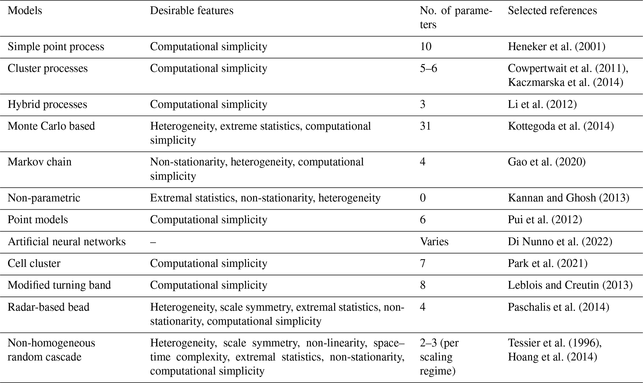
To make a literature-based assessment of these aforementioned modelling approaches in the context of using the resulting simulations as input for most hydrological applications, including the design of rainwater management infrastructures, we consider eight characteristics of observed rainfall fields that if incorporated by the framework make the simulations realistic: (1) heterogeneity: spatial heterogeneity –- rainfall is extremely variable with spatial location, especially at small spatial scales and temporal heterogeneity (intermittency) – rainfall time series at a single spatial location are extremely variable with time, especially on small timescales. (2) Physically based –- the model represents the underlying process at least abstractly using physically meaningful parameters in a slightly more generalized framework, because it is stochastic rather than deterministic, with fractional rather than integer derivatives. (3) Non-linearity –- for instance, fields are not presumed to be additive, e.g. like a Gaussian or a Lévy process, but multiplicative. The former are linear, while the latter are strongly non-linear. (4) Space–time complexity –- both spatial and temporal variability/properties of the field can be considered simultaneously, thereby incorporating possible space–time anisotropy. (5) Extreme statistics -– extreme rainfall events occur more frequently in fat-tailed distributions than in Gaussian distributions. (6) Statistical non-stationarity with the possibility of long-term memory –- the statistical properties of the field being auto-correlated over larger temporal lags. The last two characteristics that are considered for the assessment make models practically attractive. (7) High parameter parsimony –- the model uses only a few parameters. (8) Low computational complexity –- the entire simulation procedure, including parameter estimation, is not too time-consuming. The existence of simplifying physical principles such as universality helps the frameworks in being highly parsimonious and computationally simple without compromising too much on the physical relevance of the simulations. Table 1 shows a literature-based comparison of the desirable characteristics possessed by each model sub-classification. As shown in Fig. 1, most of the aforementioned models (10 out of 12) seem to be more focussed on computational and conceptual simplicity than on physics. Alternatives such as universal multi-fractal (UM) cascades that are not computationally that complicated compared to high-resolution numerical weather prediction models that explicitly represent given atmospheric processes on a limited range of scale therefore seem to be attractive choices, especially since they are capable of representing fields with high spatiotemporal variability (Schertzer and Lovejoy, 1989, 2011). These UM cascade models need only observational rainfall time series (not very data-demanding) and are computationally simpler and parsimonious compared to the radar-based bead method (Pegram and Clothier, 2001) mentioned earlier. Such UM-based procedures can also be directly extended to obtain space–time fields as well. Furthermore, the idea of space–time complexity in the UM framework is somewhat more generalized than it is in the radar-based bead model, where spatial complexity and temporal complexity are dealt with separately rather than together.
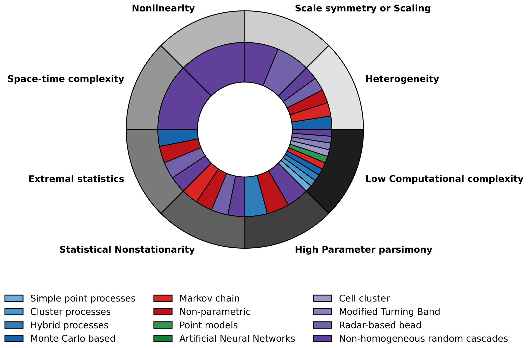
Figure 1Outer ring: desirable characteristics in stochastic high-resolution rainfall simulation models. Inner ring: models that possess these characteristics (based on Table 1). Models with ≤3 parameters are considered here to possess high parameter parsimony. Non-homogeneous random cascade models seem to possess all the desirable properties.
Table 1Comparison of different stochastic rainfall modelling procedures based on the literature.
The objective of this paper is to (i) address the general discrepancy between standard procedures for defining reference precipitation and the strong multi-scale intermittency of precipitation by making use of its extreme non-Gaussian statistics and scaling behaviour over two sub-ranges of timescales – due to earth's finite size – necessitating some adaptation of the multi-fractal modelling procedure, (ii) suggest a technique to make multi-fractal simulations have the necessary partial statistical references by defining a renormalization procedure, and (iii) to assess the accuracy of the proposed simulation method by defining multi-scale metrics that assess the closeness of observed and simulated time series across timescales. These objectives enable the generation of baseline precipitation scenarios that can be used as realistic inputs into hydrological models for applications such as the optimal design of storm-water management infrastructures, such as green roofs. Region-specific (i.e. single site separately for different sites/conurbations) reference rainfall time series characterized by the required P,D, and T properties, exhibiting larger variability and intermittency over a wide range of timescales close to that observed, are therefore simulated here for three localities in France. These simulated scenarios can therefore be considered to be more realistic than those obtained from traditional procedures that often utilize uniform rainfall or synthetic hyetograms (Qiu et al., 2021). It is worth noting that simulating just rainfall time series instead of space–time fields is justified because (i) the dichotomy between time and space–time is not as strong as usual for multi-fractal models because a multi-fractal time series can be seen as a temporal cut of a space–time multi-fractal field, (ii) the aim of the present study is focused on storm-water management over a fixed and rather small spatial area such as a building roof as mentioned earlier, and (iii) the large-scale deployment of rainfall-runoff management technologies would instead require space–time models, obtained with the help of new and rather limited developments as mentioned in (i). Section 2 discusses the different regions considered in France, their corresponding reference rainfall regulations and the observational datasets used. These rainfall datasets are analysed via multi-fractal techniques as shown in Sect. 3 to identify scaling regimes and corresponding UM parameters necessary to simulate rainfall. Section 4 gives a brief recollection about discrete-in-scale UM cascades, explains in detail the procedure used here to simulate reference rainfall scenarios and finally defines four metrics to quantitatively compare the simulations with corresponding datasets. Finally, the conclusions of this study along with its limitations and some future scopes including extension to higher dimensions and other regions are discussed in Sect. 5.
French regional storm-water management/discharge regulations mentioned in governmental rainfall zoning documents provide guidelines for reference rainfall events. Buildings/plots irrespective of the design or type of their storm-water management infrastructure are required to comply with certain drainage/discharge rules during the occurrence of such reference rainfall events. Table 2 shows the reference rainfall guidelines for three different localities in France, and it can be seen that they display high variability, but this is not that surprising since rainfall, like many other geophysical fields, exhibits high spatiotemporal variability. From the P, D, and T combinations for Nantes and Aix-en-Provence it is very clear that these specifications are highly variable for different zones within the same region. The corresponding hydrological designs therefore have to take into account such high space–time variability of rainfall, at least up to and in fact more than these legal constraints or regulations. Therefore, it is quite logical that the modelling technique to be used for stochastically simulating an ensemble of such highly variable reference rainfall scenarios should explicitly incorporate properties of heterogeneity and non-Gaussian statistics among several other properties that the observed fields typically exhibit. The rainfall datasets/time series used for the three regions, i.e. Paris, Nantes and Aix-en-Provence, were obtained from MeteoFrance (https://donneespubliques.meteofrance.fr/, last access: 4 March 2021) and were of different temporal resolutions (6 min, hourly, daily). Figure 2 shows the selected conurbations and their climatological rainfall data. These three regions were selected for this study as their monthly cumulative rainfall climatologies computed from daily datasets are quite different from each other: while Paris receives around 40–60 mm monthly rainfall, Nantes receives a higher monthly rainfall from around 40 to 90 mm, and Aix-en-Provence on the other hand receives a more variable monthly rainfall from around 10 to 80 mm. Cities are chosen here since storm-water management is more vital in urban areas due to its limited infiltration capacity. Information about the datasets used for each city/conurbation is given in Table 3. Since the proportion of data missing is low, replacing these values with zeros will probably not result in any significant change to the actual data. For the sake of simplicity, we shall henceforth refer to the daily, hourly and 6 min datasets of Paris, Nantes and Aix as PD1, PD2, PD3, ND1, ND2, ND3, AD1, AD2 and AD3 respectively.
Table 2Variability of reference rainfall regulations in the three regions considered by this study.
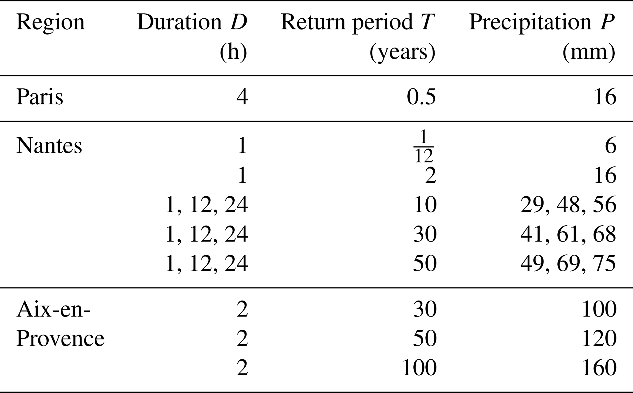
Table 3Temporal resolution, length and percentage of missing data of rainfall datasets used in this study.
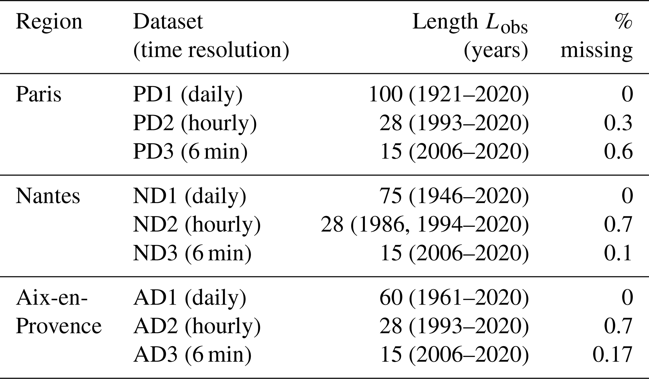
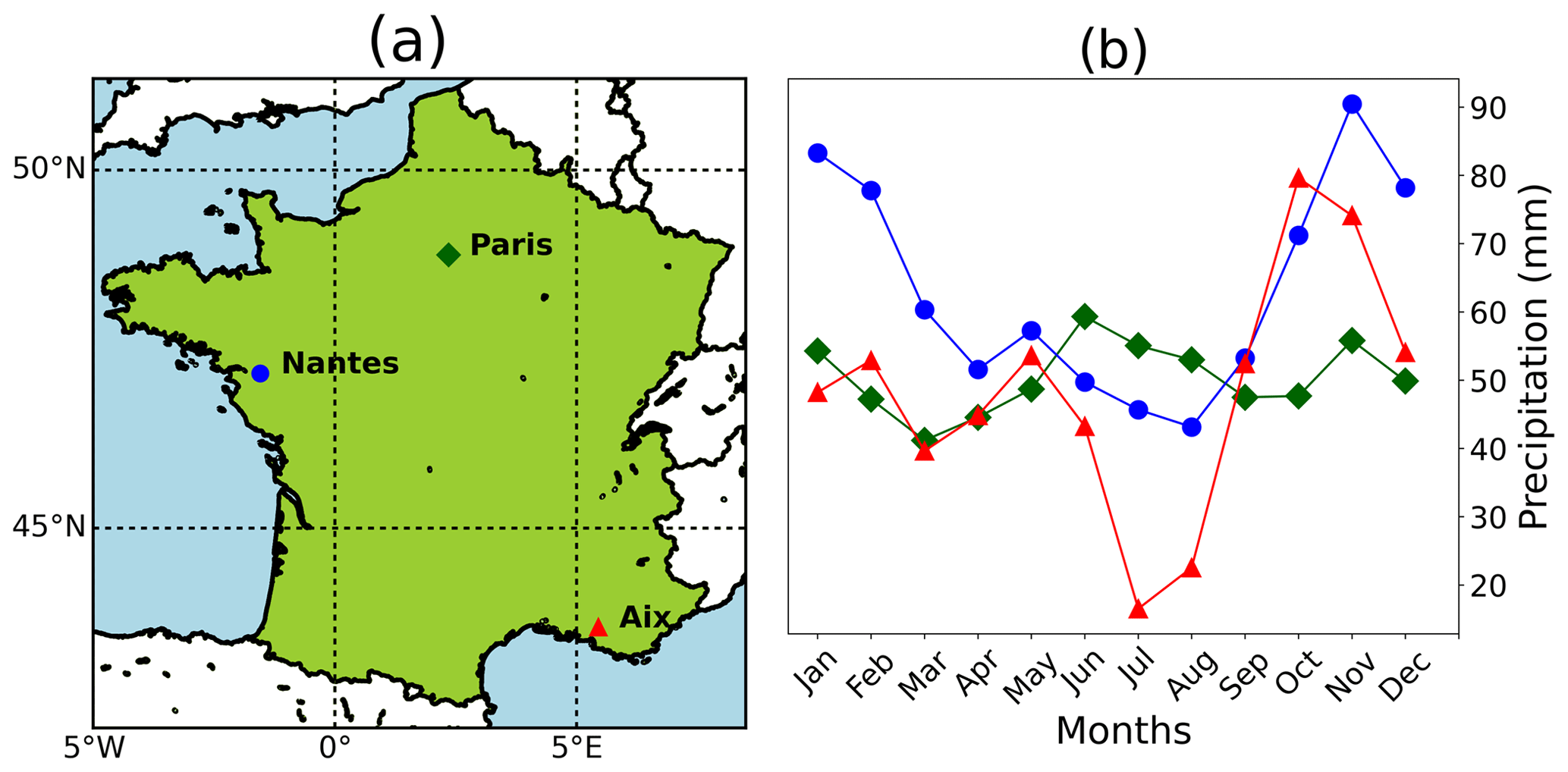
Figure 2(a) The three chosen cities/conurbations in mainland France and (b) their monthly cumulative precipitation climatology (using daily datasets).
The concept of universality in complex systems states that only a few parameters out of many are relevant for defining the system since the same dynamical process is repeated scale after scale or the process interacts with many independent processes over a range of scales, resulting in this reduction (Schertzer and Lovejoy, 1987). In the UM framework only three parameters, α, C1, and H, are necessary, and they each have different geometrical and physical meanings. The degree of multi-fractality α defines the deviation from mono-fractality, and its value is between 0 and 2. If α=0, the process is mono-/uni-fractal with a unique fractal scaling exponent, and if α=2, the process has a maximum multi-fractality with a larger spectrum of scaling exponents. The codimension of the mean C1 describes the sparseness of the level of activity that dominantly contributes to the mean field, C1=0, if the rainfall is homogeneous or, in other words, if it always rains. The parameter H quantifies the deviation from a conservative process (H=0), where the ensemble average of the field is conserved or in other words the ensemble average of the normalized field is 1. In a stochastic multi-fractal formalism, the qth-order statistical moment of rainfall Rλ observed at a scale l follows the multi-scaling equation
where λ is the intermediate scale ratio or (temporal) resolution (ratio of the largest scale to the intermediate scale l), the equality sign is used here in a scaling sense, and the scaling exponent K(q) is the scaling moment function that is scale-independent. For conservative UM, K(q) depends only on the UM parameters as follows:
By computing the trace moments and double-trace moments, the function K(q) and UM parameters can be empirically estimated (Schertzer and Lovejoy, 1987; Lavallee et al., 1993), as briefly discussed in the following two subsections. We consider each observational dataset to be a single sample to avoid any reduction in the largest scale considered, which may lead to different multi-fractal characteristics. However, there is a drawback due to this small sample size (i.e. Ns=1, making the effective dimension equal to the dimension of the time series, which is 1): the estimate of the spectral slope β is unreliable; i.e. the coefficient of determination of the straight line fit is too low. The larger the sample size, the better will be the estimate of the spectral slope (better straight line fit). Therefore, the spectral slope obtained from a time series that is split into a number of smaller samples is more reliable than that obtained from the whole time series. However, increasing sample size with a fixed dataset length means that with more samples the length of each sample is smaller, implying that there is a reduction in the largest scale considered. This may in turn lead to a difference in multi-fractal characteristics. The trace moment (TM) analysis, on the other hand, does not have this disadvantage, and the straight line fits are reasonably good and not too dependent on the number of samples. Therefore, TM analysis is simply more preferable/relevant compared to spectral analysis or estimating how many samples would be ideal when using spectral analysis. Since , consequently the H values estimated using β are also not very accurate. Therefore, H is estimated by considering the first-order (q=1) un-normalized trace moment initially assuming that the time series is non-conservative:
where once again the equality sign is used for a possible asymptotic equivalence (λ→∞).
It turns out that for all the datasets the slope of a straight line fitted through a log–log plot of vs. λ is close to zero, implying H≈0 as shown in Table 4. Therefore, we proceed by assuming that the observed rainfall time series used in this study are conservative.
Table 4UM parameter estimates for the first and second scaling regimes from different datasets (PD1 to AD3) and the scaling regimes and parameters selected for simulating rainfall over each corresponding region. H values are not included in the selected parameters and are assumed to be zero since these rain time series seem to be almost conservative (both H1 and H2 are close to zero).

3.1 TM analysis
In the TM analysis (Schertzer and Lovejoy, 1987, 1992) rainfall RΛ at the finest given (temporal) resolution or scale ratio is averaged to obtain rainfall over coarser and coarser resolutions Rλ, where the intermediate-scale ratio λ is a decreasing integer power of λ1 (), which is the scale ratio of the elementary cascade step and usually equals 2:
Since rainfall time series are multi-fractals, their statistics follow the multi-scaling Eq. (1), and therefore the trace moments at coarser and coarser (temporal) resolutions when plotted vs. λ in a log–log coordinate can be used to estimate the slope K(q) of a fitted straight line. Figure 3 shows the results of this analysis done on all the datasets (PD1 to AD3): there are two scaling regimes with a distinct slope or K(q) with a scaling break (the scale where K(q) changes abruptly and distinctly) at around 2 to 4 weeks (the synoptic maximum – due to earth's finite size). All these scaling ranges of both the first and second scaling regimes are tabulated in Table 4. Henceforth, the scaling moment functions of the first and second scaling regimes are denoted as K1(q) and K2(q) respectively. As seen from Fig. 3, the empirical statistical moments closely follow a scaling law for each moment order over a given range of resolutions, implying that it is quite reasonable to consider the observed fields to be multi-fractals.
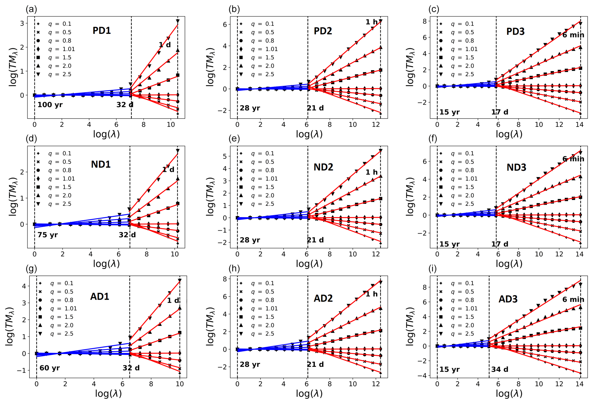
Figure 3Trace moment analysis of accumulated rainfall data. (a, b, c) Paris: PD1, PD2, PD3; (d, e, f) Nantes: ND1, ND2, ND3; (g, h, i) Aix: AD1, AD2, AD3. The first scaling regime is shown in blue, whereas the second scaling regime is shown in red.
3.2 Double-trace moment (DTM) analysis
Although the TM analysis helps in estimating K(q), it does not provide explicit estimates of UM parameters α,C1. To do this, the DTM analysis (Lavallee et al., 1993) is used:
where η is the power to which the rainfall time series is raised. Equation (5) suggests that, when K(q,η) vs. η is plotted in log–log coordinates, the slope of a fitted straight line gives the estimate of α, whereas C1 is calculated using this α estimate and the y intercept of the fitted straight line. While performing the usual DTM analysis it is found that the α estimates are larger than 2 (thereby exceeding the limits in Eq. 2) in the first scaling regime for all the datasets considered here. Generally this could be due to two different issues: (i) an incorrect α estimation procedure or (ii) an incorrect assumption about the processes' conservativeness. However, for the datasets considered here, the first possibility seems more likely due to the fact that the H estimates are negligibly small (as shown in Table 4 and discussed earlier in Sect. 3) and that Fourier analyses of these datasets are unreliable due to the small sample size chosen (Ns=1). Therefore, to overcome this issue, an iterative DTM procedure is used here. More technical details about this procedure are given in Appendix A of the Supplement. Table 4 shows the UM parameters estimated using the nine different datasets, while Fig. 4 shows the DTM-based estimation procedure. The parameters for the first and second scaling regimes are denoted by subscripts 1 and 2 respectively. Although three different scaling breaks and six different pairs of α, C1 values are empirically estimated (three pairs for each scaling regime) for each region, to simulate a reference rainfall scenario that corresponds to rainfall observed in the corresponding region, only one scaling break and two pairs of α, C1 values (one pair for each scaling regime) are necessary. Since these values are not too dependent on the dataset used, this choice is justified. The UM parameters estimated from the daily and 6 min data are selected to be used for the first and second scaling regimes in the simulations, whereas the median value of the scaling breaks (out of the three scaling breaks estimated from daily, hourly and 6 min datasets) are chosen. To confirm that this selection procedure does not result in any significant difference in the multi-fractal characteristics of the datasets and the corresponding simulations, we compute the MCI based on the difference in the theoretical maximum observable singularity from a finite-sized sample γs (Hubert et al., 1993; Douglas and Barros, 2003)
based on the difference between UM parameter values observed from datasets and selected for simulations (as indicated by the subscripts obs and sel) with the analytical expression
with respect to α and C1; the indices i,j denote the scaling regime (first or second) and the dataset (6 min, hourly or daily) used respectively. Since 0≤α≤2 and 0≤C1≤1 due to the assumption of a single sample, this implies that the maximum and minimum values of γs are close to 1 and 0 respectively.
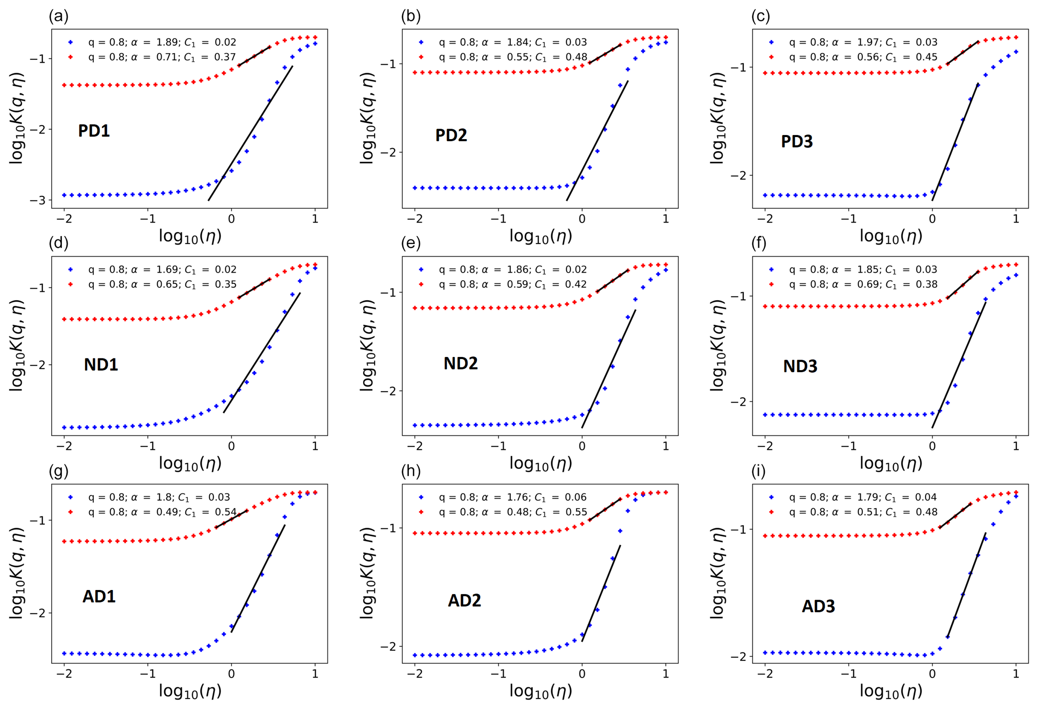
Figure 4Double trace moment analysis of accumulated rainfall data to obtain UM parameter estimates. (a, b, c) Paris: PD1, PD2, PD3; (d, e, f) Nantes: ND1, ND2, ND3; (g, h, i) Aix: AD1, AD2, AD3. The first scaling regime is shown in blue, whereas the second scaling regime is shown in red.
The MCI is computed to be 0.03 for both Paris and Nantes and 0.04 for Aix. These low values of MCI justify the aforementioned selection procedure. Multi-fractal (statistical) analyses of observed rainfall in the three conurbations chosen by this study do not display any significant seasonality as there is no scaling break around a few months' timescale. However, there is clear evidence of a strong synoptic maximum indicated by a scaling break around a few weeks' timescale with corresponding changes in scaling behaviour as seen in Fig. 3. It is worth noting that this aforementioned absence of seasonality in multi-fractal characteristics could imply that the low-frequency scaling regime's UM parameters are sufficient to represent seasonal variability (in cumulative precipitations – Fig. 2), whereas together with the high-frequency scaling regime's UM parameters they are sufficient for reproducing well the statistics of different storm types (either convective or stratiform). This requires some elaboration of the UM cascade process (as detailed in Sect. 4) to guarantee good agreement between observed and simulated rainfall over the full range of timescales.
Multi-fractal cascade processes have strongly non-Gaussian statistics (e.g. fat-tailed distributions) and therefore are capable of generating structures of highly varying intensities. These cascades represent the atmospheric physical processes underlying rainfall generation in an abstract (Richardson’s idea of energy transfer from large to small scales by random breakups of eddies) but explicit manner by the concept of scale symmetry or scale invariance – a property respected “even” by the Navier–Stokes equations used by state-of-the-art NWP models for operational weather forecasting but only on a limited range of scales (Schertzer and Lovejoy, 1987). These cascade models are based on Richardson’s idea of energy transfer embodied in his 1922 poem “Big whorls have little whorls Which feed on their velocity, And little whorls have lesser whorls And so on to viscosity.” So, the ideology of cascade models is firmly rooted in the so-called physical world while generating fields that have the right statistical properties. Therefore, these cascade models take us from the physical world to the statistical world due to which these types of models can be considered a bridge between purely statistical and purely physical models. The importance of this type of bridge has gained recognition from the Nobel Committee for Physics (Schertzer and Nicolis, 2022). Due to their multiplicative property, the heterogeneity of the simulated field increases incrementally at smaller scales (making these models capable of generating scale-dependent rain rates as observed in nature). Although discrete-in-scale cascades consider scale ratios that are integer powers of integers, they exhibit better scaling properties and are pedagogically straightforward compared to continuous-in-scale cascades (Lovejoy and Schertzer, 2010). Furthermore, for the current purpose of simulating rainfall time series, anisotropic and vector generalizations are not very relevant. Therefore, the discrete-in-scale UM cascade model is used here to simulate an ensemble of rainfall scenarios for each region with its corresponding P, D and T specifications. The basic idea of discrete-in-scale cascades (Schertzer and Lovejoy, 1989, 2011) is to iteratively divide large-scale eddies (structures) using a constant integer-scale (timescale) ratio λ1 (usually 2 as mentioned earlier) and multiplicatively distributed flux (ελ) to these sub-eddies randomly. It is convenient to do this using an additive noise or generator Γλ, the exponential of which results in the multiplicatively modulated multi-fractal flux series at (temporal) resolution λ (Schertzer and Lovejoy, 1989). To simulate universal multi-fractals (whose statistics are governed by Eqs. 1 and 2), this generator must satisfy
To do this, an extremal Lévy random variable of index α and suitable amplitude (Pecknold et al., 1993; Gires et al., 2013) – that is a function of C1 – is chosen as Γλ. This generator generates the singularity γλ corresponding to each sub-eddy. In the present context rainfall Rλ accumulated in a given interval of time is the flux ελ. Such a simulated field when normalized by its ensemble average is canonically conserved.
4.1 Simulating reference rainfall scenarios
To have the same P, D and T characteristics of the reference rainfall, a simulated rainfall series with the largest (temporal) scale (Tsim) needs to have a specific number (ρ) of peak values of rainfall (≥P) accumulated over specific durations (D) so that their return period . A simple way to do this is to multiply the simulated multi-fractal time series (with the largest scale ) by an appropriate renormalization constant (RC): P divided by the ρth highest value in the multi-fractal series aggregated over duration D. Therefore, the simulated rainfall series are dependent on these P, D and T values, resulting in 1 rainfall series for Paris, 11 rainfall series for Nantes and 3 rainfall series for Aix. Since the observed datasets have two scaling regimes, it is necessary to use a double cascade: a coarser (temporal) resolution cascade using parameters α1, for the first scaling regime and a finer (temporal) resolution cascade using parameters α2, for the second scaling regime. Let the smallest scale observed and simulated be δ (here δ=6 min for all three regions). The largest temporal scale selected from the observed datasets Tsel is related to the largest scale that can be simulated T(s,sim) (the largest scale in the simulated sample which is a power of λ1=2 and ≤Tsim):
where ⌊x⌋ denotes the integer part of x.
The coarse-resolution cascade produces a multi-fractal time series where and are the simulated scaling break. Each rainfall value of this coarse time resolution multi-fractal series is now the parent structure of the second (fine time resolution) cascade that proceeds from TB,sim up to δ. A multi-fractal time series where is thus finally produced by the double-cascade simulation (DCS). The DCS is repeated a sufficient number of times (if ) to finally extract a time series where (here δ=6 min). The ρth highest value in a aggregated multi-fractal series ( aggregated to temporal resolution ) when multiplied by RC should equal P. If we rank the values in series in decreasing order and call them , then the ρth value is the ρth highest value. Therefore, RC is computed as
The RC computed using Eq. (10) when multiplied by gives the final rainfall series that has characteristics corresponding to the reference rainfall. This entire procedure is repeated ne times to generate an ne-member ensemble of possible reference rainfall scenarios (Fig. 5 schematically presents the whole temporal simulation method). Here, ne=10, i.e. an ensemble of 10 members (m1 to m10), is simulated.
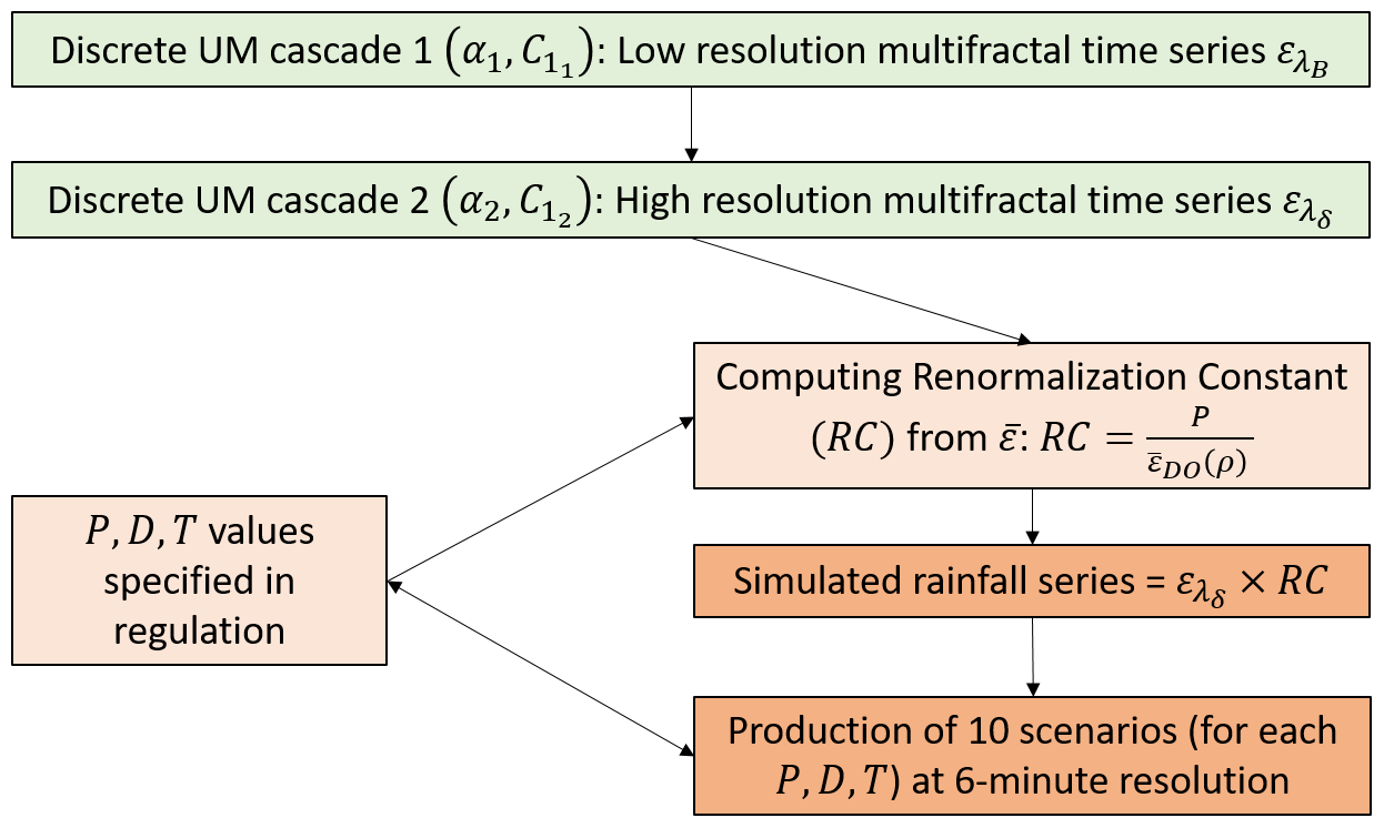
Figure 5Schematic illustration of the simulation procedure used in this study to generate temporal reference rainfall scenarios.
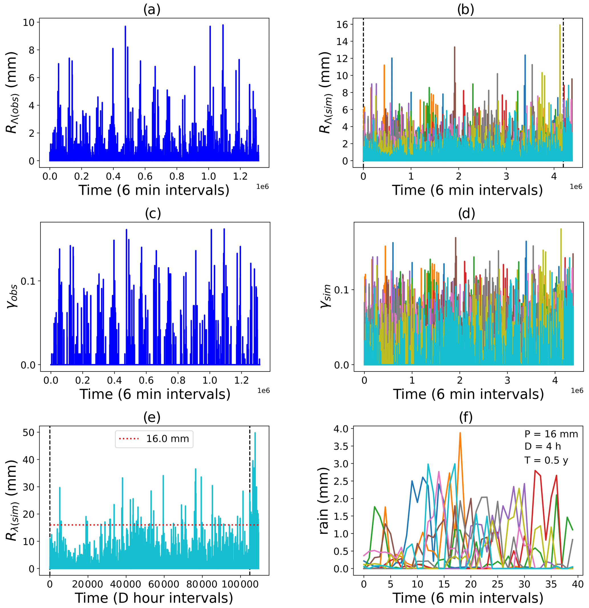
Figure 6Paris reference rainfall scenarios (). (a) Rainfall and (c) corresponding singularities from observational dataset PD3. (b) Rainfall, (d) corresponding singularities, (e) aggregated rainfall from member m10 and (f) events with 16 mm cumulative rainfall of 4 h duration from the ensemble double-cascade simulation.
Figure 6 shows the reference rainfall simulations for Paris: both rainfall data and singularities can be compared from the figure. The maximum observed and simulated singularities are closer to each other than that of the corresponding rainfall values. This may be attributed to the fact that singularities are less scale-dependent than rainfall and that the observed and simulated rainfall have different scale ratios (resulting in the unreliability of comparisons using parameters that are more scale-dependent) since their largest scales are different in spite of their smallest scales being equal. Figure 6e shows that the simulated rainfall (from one member of the ensemble: m10) obeys the P, D, and T reference criteria for the Paris region. To highlight the internal variability of the 10 reference rainfall scenarios simulated, events where exactly P mm of rainfall occurs within D hours' duration are plotted separately in Fig. 6f). Figures A1 and A2 in the Supplement are the same as Fig. 6f) but are for different P, D and T specifications of Nantes and Aix-en-Provence.
4.2 Comparing simulations with observational datasets
Four metrics possessing different properties have been defined to compare the stochastic simulations of rainfall to the actual datasets. The first metric is the multi-fractal comparison metric (MCM), the second metric is the rainfall comparison metric (RCM), the third metric is the singularity comparison metric (SCM) and the fourth and final metric is the codimension comparison metric (CCM). These metrics are defined with the general idea that the lower metrics correspond to better simulations and vice versa.
4.2.1 MCM
The MCM is a theoretical metric and is computed based on the maximum observable theoretical singularity γs (Eq. 7) from a finite sample size , where DS is the sample dimension (Schertzer and Lovejoy, 1992) in each dataset and in each simulated member of the ensemble
where j indicates the dataset used (daily, hourly or 6 min), i denotes the scaling regime (first or second), k indicates the ensemble member. MCM is closely related to MCI defined earlier, the only difference between them is that the MCM uses the UM parameters estimated from DTM analysis of simulated members, whereas MCI directly uses the UM parameters selected for simulations from the observed datasets. Therefore, as expected the MCM computed for all the simulations are very low (shown in Fig. 7) and close to MCI. Since both the MCM and MCI depend only on the UM parameters or in other words the multi-fractal characteristics of the series, they are scale-independent. This means that the MCM of two time series of same or different temporal resolutions or lengths are not too different. Since renormalization does not affect the multi-fractal properties of a series, the MCM is independent of P, D and T. Lower values of the MCM imply that the simulation has multi-fractal properties close to that of observed data.
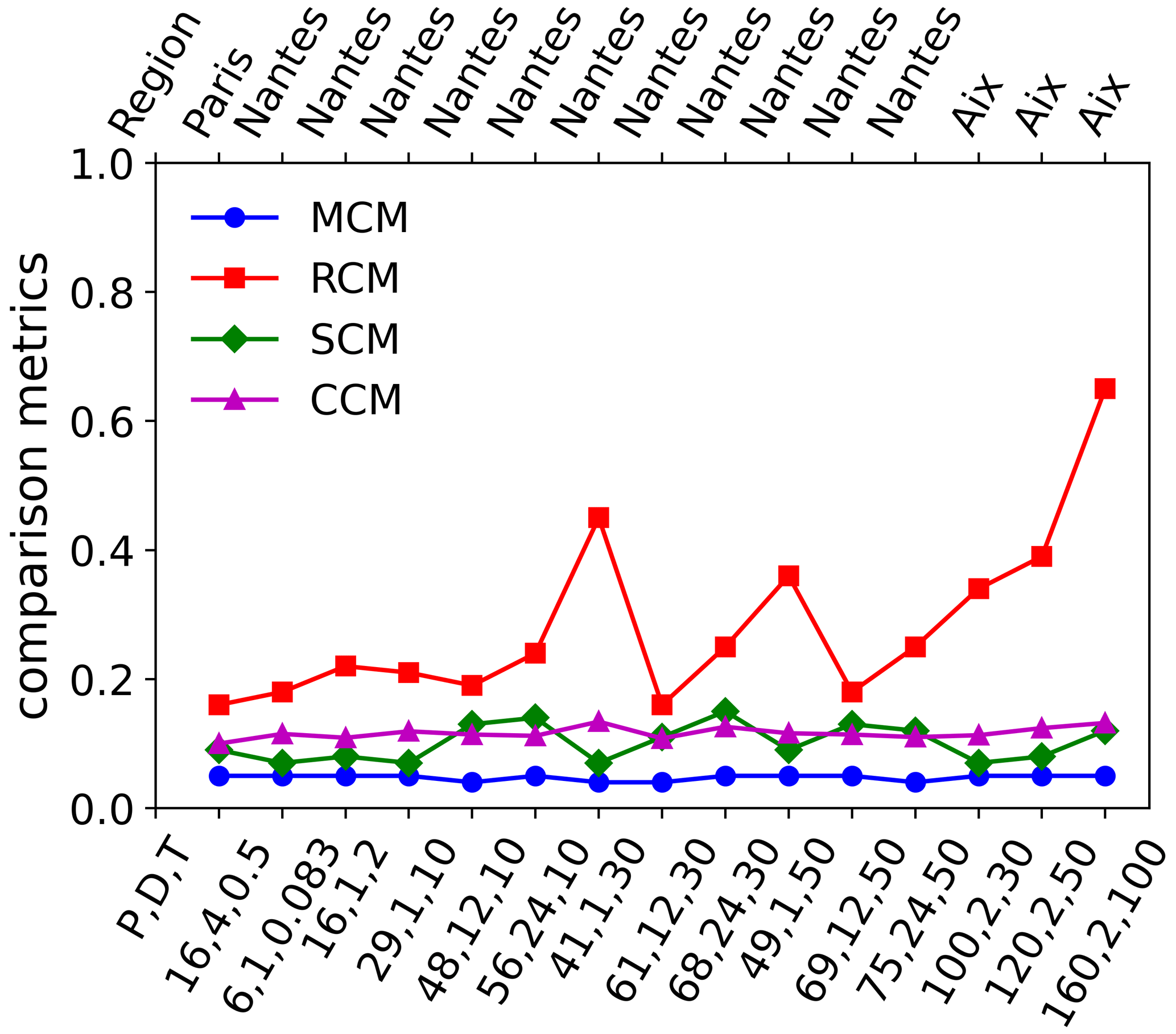
Figure 7Multi-fractal comparison metric, rainfall comparison metric, singularity comparison metric and codimension comparison metric for all the different reference rainfall simulations. P, D, and T are in units of mm, hours and years respectively.
4.2.2 RCM
The RCM on the other hand is a more practical metric and is computed based on the highest rainfall value present in the dataset and in each simulation member:
where ; ; δ(j)=1 d,1 h,6 min for , the indices j,k have the same meaning as in the MCM.
Lower values of the RCM imply that the extreme behaviour of simulations are closer to that of the observed data. However, RCM is sensitively dependent on scale and P, D, T. Therefore, as shown in Fig. 7, the RCM values are larger for cases where is larger. This might be due to the fact that the datasets used, because of their shorter lengths are not actually representative of these specific P, D, T values that correspond to rainfall events that are more extreme, since the probability of observing rarer events is higher in larger datasets.
4.2.3 SCM
The SCM is a metric that, instead of comparing the actual time series, compares the singularities corresponding to them and is computed as
where ; , the indices j,k have the same meaning as in the MCM.
Lower values of SCM imply that the simulations are closer to the observations (after reducing the effect of scale dependence on the comparison) since the singularities corresponding to the simulations and the singularities corresponding to the observations are close to each other. Although SCM is scale-dependent it is less sensitive to scale than RCM; moreover SCM is also dependent on P, D, T. Therefore, SCM values of all simulations are low (≤0.15) even for cases where is larger as shown in Fig. 7.
4.2.4 CCM
The main drawbacks of the MCM, RCM and SCM are that they focus only on either the maximum rainfall values or the maximum singularities. By contrast, a range of values rather than threshold values can be used. For instance, the codimension of singularity c(γ) takes into account a range of singularities larger than γ, following Schertzer and Lovejoy 1987,
meaning that c(γ) can be obtained as the negative of the slope of a straight line fitted to log–log plot of Pr [Rλ≥λγ] with respect to λ. Equation (14) (where ≈ indicates an asymptotic equivalence) implies that c(γ) is almost scale independent and any metric defined using it should also be not very scale-sensitive. The CCM is defined as
where γΛ(obs(j))(i) , the indices j,k have the same meaning as in the MCM, whereas i indexes the singularities (here n=10 singularities are used for the comparison procedure).
The CCM is dependent on P, D, T via the singularities γΛ, therefore in an almost scale-independent manner. As shown in Fig. 7, the SCM and CCM values are consistently low, implying that it is possible to simulate reference rainfall ensembles characterized by the required properties while taking into account temporal variability. It is worth noting here that autocorrelation or its inverse Fourier transform i.e. spectral density are generally just second order statistics. Comparing the scaling moment function K(q) for q=2 of observed and simulated rainfall is the same as comparing their respective spectra and therefore their autocorrelation. The CCM compares c(γ) instead of K(q) since they are just the Legendre transforms of each other and each order of singularity γ corresponds to an order of statistical moment q. Therefore, the CCM is a more generalized metric as it readily considers the second-order statistics and more.
The α,C1 estimates for the second scaling regime and the scaling breaks listed in Table 4 are quite comparable with those of earlier studies (Hubert et al., 1993; Ladoy et al., 1993). These breaks in temporal scaling can be attributed to the synoptic maximum (Tessier et al., 1996) or in other words the lifetime of planetary-scale atmospheric structures. The similarity of scaling breaks observed in all the datasets justifies the dependence of the scaling break on the value of the largest planetary spatial scale and its corresponding eddy turnover time or lifetime. Furthermore, like in earlier studies (Hoang et al., 2014), the negligible H estimates suggest that the process is conservative in both scaling regimes. It can be seen that, while the first, low-frequency scaling regime has a larger α and a smaller C1, the reverse is true for the second, high-frequency scaling regime. A similar pattern seems to be followed for all three conurbations irrespective of the dataset considered in this study. For a conservative process, this seemingly inverse relation between α and C1 could be reasoned as follows: a larger C1 value implies that the processes contributing dominantly to the mean occur rarely, since the probability of the occurrence of singularities contributing to the mean is highest; this in turn implies that other singularities occur even more rarely or in other words the range of singularities is rather limited, resulting in the process having a reduced degree of multi-fractality, i.e. smaller α values. On the other hand, C1 values close to 0 in the low-frequency scaling regime could be because at timescales larger than the synoptic maximum it can be expected to rain almost always. Comparing the UM parameter estimates in the corresponding scaling regimes of all three conurbations, it can be seen that they are somewhat similar to one another. Similarity of the parameter values confirms that rainfall at the three different locations has some common properties, e.g. intermittency. At the same time, small differences in parameter values can result in significant changes in the probability of occurrence of events exceeding a given threshold and therefore possible location-dependent processes, for instance, different levels of intermittency. Based on the above discussion, it seems that the rainfall can be considered to be the most intermittent (i) over smaller timescales in Aix, closely followed by Paris and finally by Nantes, and (ii) over larger timescales in Aix, closely followed by both Paris and Nantes. This might at least partially explain why the reference rainfall rules for Aix seem to be too focused on extreme rainfall events, as seen in Table 2.
The classical UM framework does not address seasonality because it assumes a form of statistical stationarity. However, this framework can be generalised to include a given type of seasonality (Tchiguirinskai et al., 2007). To keep the present paper as focused as possible, we only wanted to take into account a question on possible biases of UM simulation vs. empirical data due to the difference of periodicity. This is why we use this simple indicator , which when close to 0 implies that the time gap, i.e. the number of months nms between the maximum and minimum monthly rainfall, is similar for both observed and simulated rainfall. From Fig.2b it can be seen that nms,obs for all the three conurbations is 2, and from the simulated scenarios it is found that nms,sim for Paris, Nantes and Aix are 2.3,1.8 and 2.6 respectively, resulting in the following indicator values for Paris, Nantes and Aix: 0.027,0.018 and 0.055, which are closer to 0 than to 1. With respect to the traditional coefficient of variation, this simple indicator has the advantage of not being limited to quasi-Gaussian/second-order statistics.
The idea of defining the comparison metrics was to make a quantitative, robust yet quick comparison of the simulations with observed datasets, and they seem quite adequate considering the objective of this paper. It should be noted that these metrics (MCM, SCM, CCM) are defined across scales, unlike the usual scores (such as RCM) which are limited to the estimation of a given scale. One main limitation in this paper is that of discrete UM cascades, since they use integer scale ratios which can be considered to be a non-physical assumption. The method proposed here can only do what it was developed for, i.e. simulating realistic reference rainfall scenarios to design storm-water management infrastructure. Simulating rainfall in real time and/or forecasting rain is not the goal of this method. Furthermore, it cannot be used directly to simulate additional related variables such as temperature that could be relevant in the design of urban storm-water management devices including green roofs.
Even though several earlier studies have attempted to simulate rainfall using a UM approach, we are unaware of UM-based studies that have proposed procedures to simulate reference rainfall scenarios. A novel method is proposed here to simulate reference rainfall scenarios that are indispensable for hydrological applications, such as designing green roofs and other generic storm-water management devices. The suggested discrete-in-scale universal multi-fractal cascade-based method is used here to stochastically simulate an ensemble of reference rainfall scenarios with rainfall events exceeding or equal to P mm within D hours' duration with a return period of T years as specified by regional storm-water management regulations for three conurbations in France. The extreme variability of P, D and T values, which is a direct result of the extreme space–time variability of precipitation and the underlying atmospheric processes, not only justifies, but also makes the choice of UM framework rather crucial in producing computationally cheap, realistic reference rainfall ensembles that have the right statistics and probably the right physics due to its physically meaningful parameters. Furthermore, four new metrics are proposed to quantify the performance of the suggested procedure and analyse their effectiveness. The three metrics (MCM, SCM and CCM), which are not too scale-dependent, seem to indicate that the simulations are good. CCM being almost scale-independent and utilizing a range of values rather than just maxima for comparison seems to be the most reliable comparison metric. Therefore, the consistently low CCMs show that the proposed method is indeed an attractive choice to stochastically simulate physically based reference rainfall scenarios. Although only purely temporal, discrete-in-scale, conservative simulations over Paris, Nantes and Aix are considered in this study, this approach could possibly be generalized to spatiotemporal, continuous-in-scale, non-conservative simulations over other locations as well. While it is true that the proposed approach is for hydrological applications such as designing green roofs for rainwater management, observational data of not only rainfall, but also discharge from the green roof, will be necessary to validate the entire hydro-meteorological modelling approach. This would require the setting up of experimental green roof prototypes designed using green roof models capable of simulating the hydrological behaviour of both substrate and drainage layers with reference rainfall scenarios as input and defining metrics that quantify compliance with regulations. These prototypes can then be monitored to estimate how much they comply with discharge rules via the compliance metrics. All these elements will therefore be the subjects of separate publications in future.
The code used here along with other multi-fractal tools will be consolidated into a Python library (MFPL) that can be publicly accessed on GitHub.
The data sets used here can be obtained by applying for them at the MeteoFrance website (https://donneespubliques.meteofrance.fr/, last access: 4 March 2021).
The supplement related to this article is available online at: https://doi.org/10.5194/hess-26-6477-2022-supplement.
AR performed the study and prepared the manuscript, PAV and DS supervised the work, IT provided vital suggestions, and RP and LS helped in gaining insights into commercial hydro-meteorological applications.
The contact author has declared that none of the authors has any competing interests.
Publisher’s note: Copernicus Publications remains neutral with regard to jurisdictional claims in published maps and institutional affiliations.
The authors thank MeteoFrance for providing the in situ rainfall observational datasets used in this study.
This research has been co-supported in the framework of the convention linking SOPREMA and ENPC (convention no. R-2019-0525).
This paper was edited by Nadav Peleg and reviewed by three anonymous referees.
Arnaud, P. and Lavabre, J.: Nouvelle approche de la prédétermination des pluies extrêmes, Comptes Rendus de l'Académie des Sciences – Series IIA – Earth and Planetary Science, 328, 615–620, https://doi.org/10.1016/S1251-8050(99)80158-X, 1999. a
Berenguer, M., Sempere-Torres, D., and Pegram, G. G.: SBMcast – An ensemble nowcasting technique to assess the uncertainty in rainfall forecasts by Lagrangian extrapolation, J. Hydrol., 404, 226–240, https://doi.org/10.1016/j.jhydrol.2011.04.033, 2011. a
Brandsma, T. and Buishand, T. A.: Simulation of extreme precipitation in the Rhine basin by nearest-neighbour resampling, Hydrol. Earth Syst. Sci., 2, 195–209, https://doi.org/10.5194/hess-2-195-1998, 1998. a
Burian, S. J., Durrans, S. R., Nix, S. J., and Pitt, R. E.: Training Artificial Neural Networks to Perform Rainfall Disaggregation, J. Hydrol. Eng., 6, 43–51, https://doi.org/10.1061/(ASCE)1084-0699(2001)6:1(43), 2001. a
Cameron, D., Beven, K., and Tawn, J.: Modelling extreme rainfalls using a modified random pulse Barlett-Lewis stochastic rainfall model (with uncertainly), Adv. Water Resour., 24, 203–211, https://doi.org/10.1016/S0309-1708(00)00042-7, 2000a. a
Cameron, D., Beven, K., and Tawn, J.: An evaluation of three stochastic rainfall models, J. Hydrol., 228, 130–149, https://doi.org/10.1016/S0022-1694(00)00143-8, 2000b. a
Cowpertwait, P. S.: Generalized point process model for rainfall, P. Roy. Soc. Lond. A Mat., 447, 23–37, https://doi.org/10.1098/rspa.1994.0126, 1994. a
Cowpertwait, P. S. P., O'Connell, P. E., Metcalfe, A. V., and Mawdsley, J. A.: Stochastic point process modelling of rainfall. II. Regionalisation and disaggregation, J. Hydrol., 175, 47–65, https://doi.org/10.1016/S0022-1694(96)80005-9, 1996. a
Cowpertwait, P. S. P., Xie, G., Isham, V., Onof, C., and Walsh, D. C. I.: A fine-scale point process model of rainfall with dependent pulse depths within cells, Hydrolog. Sci. J., 56, 1110–1117, https://doi.org/10.1080/02626667.2011.604033, 2011. a, b
Di Nunno, F., Granata, F., Pham, Q. B., and de Marinis, G.: Precipitation Forecasting in Northern Bangladesh Using a Hybrid Machine Learning Model, Sustainability, 14, 1–21, https://doi.org/10.3390/su14052663, 2022. a, b
Douglas, E. M. and Barros, A. P.: Probable Maximum Precipitation Estimation Using Multifractals: Application in the Eastern United States, J. Hydrometeorol., 4, 1012–1024, https://doi.org/10.1175/1525-7541(2003)004<1012:PMPEUM>2.0.CO;2, 2003. a
Gao, C., Booij, M. J., and Xu, Y.-P.: Development and hydrometeorological evaluation of a new stochastic daily rainfall model: Coupling Markov chain with rainfall event model, J. Hydrol., 589, 125337, https://doi.org/10.1016/j.jhydrol.2020.125337, 2020. a, b
Gao, C., Guan, X., Booij, M. J., Meng, Y., and Xu, Y.-P.: A new framework for a multi-site stochastic daily rainfall model: Coupling a univariate Markov chain model with a multi-site rainfall event model, J. Hydrol., 598, 126478, https://doi.org/10.1016/j.jhydrol.2021.126478, 2021. a
Gholami, V., Darvari, Z., and Mohseni Saravi, M.: Artificial neural network technique for rainfall temporal distribution simulation (Case study: Kechik region), Caspian Journal of Environmental Sciences, 13, 53–60, 2015. a
Gires, A., Tchiguirinskaia, I., Schertzer, D., and Lovejoy, S.: Development and analysis of a simple model to represent the zero rainfall in a universal multifractal framework, Nonlin. Processes Geophys., 20, 343–356, https://doi.org/10.5194/npg-20-343-2013, 2013. a
Gyasi-Agyei, Y.: Stochastic disaggregation of daily rainfall into one-hour time scale, J. Hydrol., 309, 178–190, https://doi.org/10.1016/j.jhydrol.2004.11.018, 2005. a
Gyasi-Agyei, Y. and Willgoose, G. R.: Generalisation of a hybrid model for point rainfall, J. Hydrol., 219, 218–224, https://doi.org/10.1016/S0022-1694(99)00054-2, 1999. a
Heneker, T. M., Lambert, M. F., and Kuczera, G.: A point rainfall model for risk-based design, J. Hydrol., 247, 54–71, https://doi.org/10.1016/S0022-1694(01)00361-4, 2001. a, b
Hoang, C. T., Tchiguirinskaia, I., Schertzer, D., and Lovejoy, S.: Caractéristiques multifractales et extrêmes de la précipitation à haute résolution, application à la détection du changement climatique, Revue des Sciences de l'Eau, 27, 205–216, https://doi.org/10.7202/1027806ar, 2014. a, b
Hubert, P., Tessier, Y., Lovejoy, S., Schertzer, D., Schmitt, F., Ladoy, P., Carbonnel, J. P., Violette, S., and Desurosne, I.: Multifractals and extreme rainfall events, Geophys. Res. Lett., 20, 931–934, https://doi.org/10.1029/93GL01245, 1993. a, b
Kaczmarska, J., Isham, V., and Onof, C.: Point process models for fine-resolution rainfall, Hydrolog. Sci. J., 59, 1972–1991, https://doi.org/10.1080/02626667.2014.925558, 2014. a, b
Kannan, S. and Ghosh, S.: A nonparametric kernel regression model for downscaling multisite daily precipitation in the Mahanadi basin, Water Resour. Res., 49, 1360–1385, https://doi.org/10.1002/wrcr.20118, 2013. a, b
Kottegoda, N., Natale, L., and Raiteri, E.: Monte Carlo Simulation of rainfall hyetographs for analysis and design, J. Hydrol., 519, 1–11, https://doi.org/10.1016/j.jhydrol.2014.06.041, 2014. a, b
Koutsoyiannis, D. and Onof, C.: Rainfall disaggregation using adjusting procedures on a Poisson cluster model, J. Hydrol., 246, 109–122, https://doi.org/10.1016/S0022-1694(01)00363-8, 2001. a
Ladoy, P., Schmitt, F., Schertzer, D., and Lovejoy, S.: The multifractal temporal variability of Nimes rainfall data, Comptes Rendus – Academie des Sciences, Serie II, Vol. 317, 775–782, Reports of the Academy of Sciences Series 2 Mechanics Physics Chemistry Earth and Universe Sciences (France), 1993. a
Lavallee, D., Lovejoy, S., Schertzer, D., and Ladoy, P.: Nonlinear variability of landscape topography: multifractal analysis and simulation, Fractals in geography, edited by: De Cola, L. and Lam, N., 158–192, PTR Prentice Hall, ISBN 0131058673, 1993. a, b
Leblois, E. and Creutin, J.-D.: Space-time simulation of intermittent rainfall with prescribed advection field: Adaptation of the turning band method, Water Resour. Res., 49, 3375–3387, https://doi.org/10.1002/wrcr.20190, 2013. a, b
Li, C., Singh, V. P., and Mishra, A. K.: Simulation of the entire range of daily precipitation using a hybrid probability distribution, Water Resour. Res., 48, https://doi.org/10.1029/2011WR011446, 2012. a, b
Lovejoy, S. and Schertzer, D.: On the simulation of continuous in scale universal multifractals, Part II: Space-time processes and finite size corrections, Comput. Geosci., 36, 1404–1413, https://doi.org/10.1016/j.cageo.2010.07.001, 2010. a
Mehrotra, R. and Sharma, A.: A nonparametric stochastic downscaling framework for daily rainfall at multiple locations, J. Geophys. Res.-Atmos., 111, 1–16, https://doi.org/10.1029/2005JD006637, 2006. a
Nerini, D., Besic, N., Sideris, I., Germann, U., and Foresti, L.: A non-stationary stochastic ensemble generator for radar rainfall fields based on the short-space Fourier transform, Hydrol. Earth Syst. Sci., 21, 2777–2797, https://doi.org/10.5194/hess-21-2777-2017, 2017. a
Onof, C., Chandler, R. E., Kakou, A., Northrop, P., Wheater, H. S., and Isham, V.: Rainfall modelling using poisson-cluster processes: A review of developments, Stoch. Env. Res. Risk A., 14, 384–411, https://doi.org/10.1007/s004770000043, 2000. a
Park, J., Cross, D., Onof, C., Chen, Y., and Kim, D.: A simple scheme to adjust Poisson cluster rectangular pulse rainfall models for improved performance at sub-hourly timescales, J. Hydrol., 598, 126296, https://doi.org/10.1016/j.jhydrol.2021.126296, 2021. a, b
Paschalis, A., Molnar, P., Fatichi, S., and Burlando, P.: A stochastic model for high-resolution space-time precipitation simulation, Water Resour. Res., 49, 8400–8417, https://doi.org/10.1002/2013WR014437, 2013. a
Paschalis, A., Fatichi, S., Molnar, P., Rimkus, S., and Burlando, P.: On the effects of small scale space–time variability of rainfall on basin flood response, J. Hydrol., 514, 313–327, https://doi.org/10.1016/j.jhydrol.2014.04.014, 2014. a, b
Pathirana, A. and Herath, S.: Multifractal modelling and simulation of rain fields exhibiting spatial heterogeneity, Hydrol. Earth Syst. Sci., 6, 695–708, https://doi.org/10.5194/hess-6-695-2002, 2002. a
Pecknold, S., Lovejoy, S., Schertzer, D., Hooge, C., and Malouin, J. F.: The simulation of universal multifractals, 228–267, World Scientific, ISBN 978-981-4553-21-6, 1993. a
Pegram, G. G. S. and Clothier, A. N.: High resolution space–time modelling of rainfall: the “String of Beads” model, J. Hydrol., 241, 26–41, https://doi.org/10.1016/S0022-1694(00)00373-5, 2001. a, b
Pui, A., Sharma, A., Mehrotra, R., Sivakumar, B., and Jeremiah, E.: A comparison of alternatives for daily to sub-daily rainfall disaggregation, J. Hydrol., 470-471, 138–157, https://doi.org/10.1016/j.jhydrol.2012.08.041, 2012. a, b
Qiu, Y., da Silva Rocha Paz, I., Chen, F., Versini, P.-A., Schertzer, D., and Tchiguirinskaia, I.: Space variability impacts on hydrological responses of nature-based solutions and the resulting uncertainty: a case study of Guyancourt (France), Hydrol. Earth Syst. Sci., 25, 3137–3162, https://doi.org/10.5194/hess-25-3137-2021, 2021. a
Rajagopalan, B. and Lall, U.: A k-nearest-neighbor simulator for daily precipitation and other weather variables, Water Resour. Res., 35, 3089–3101, https://doi.org/10.1029/1999WR900028, 1999. a
Salas, J.: Analysis and modeling of hydrologic time series, Handbook of hydrology, ISBN 0070397325, edited by: Maidment, D. R., 1993. a
Schertzer, D. and Lovejoy, S.: Physical modeling and analysis of rain and clouds by anisotropic scaling mutiplicative processes, J. Geophys. Res., 92, 9693–9693, https://doi.org/10.1029/JD092iD08p09693, 1987. a, b, c, d, e
Schertzer, D. and Lovejoy, S.: Multifractal simulations and analysis of clouds by multiplicative processes, Atmos. Res., 21, 337–361, https://doi.org/10.1016/0169-8095(88)90035-X, 1988. a
Schertzer, D. and Lovejoy, S.: Nonlinear Variability in Geophysics: Multifractal Simulations and Analysis, in: Fractals' Physical Origin and Properties, Springer New York, NY, https://doi.org/10.1007/978-1-4899-3499-4-3, 1989. a, b, c, d
Schertzer, D. and Lovejoy, S.: Hard and soft multifractal processes, Physica A, 185, 187–194, https://doi.org/10.1016/0378-4371(92)90455-Y, 1992. a, b
Schertzer, D. and Lovejoy, S.: Multifractals, Generalized Scale Invariance and Complexity in geophysics, Int. J. Bifurcat. Chaos, 21, 3417–3456, https://doi.org/10.1142/S0218127411030647, 2011. a, b
Schertzer, D. and Nicolis: Nobel Recognition for the Roles of Complexity and Intermittency, http://eos.org/opinions/nobel-recognition-for-the-roles-of-complexity-and-intermittency, last access: 15 December 2022. a
Serinaldi, F.: Multifractality, imperfect scaling and hydrological properties of rainfall time series simulated by continuous universal multifractal and discrete random cascade models, Nonlin. Processes Geophys., 17, 697–714, https://doi.org/10.5194/npg-17-697-2010, 2010. a
Shah, S., O'Connell, P., and Hosking, J.: Modelling the effects of spatial variability in rainfall on catchment response. 1. Formulation and calibration of a stochastic rainfall field model, J. Hydrol., 175, 67–88, https://doi.org/10.1016/S0022-1694(96)80006-0, 1996. a
Tchiguirinskai, I., Schertzer, D., Hubert, P., Bendjoudi, H., and Lovejoy, S.: Potential of multifractal modelling of ungauged basins, p. 11, edited by: Schertzer, D., Hubert, P., Koide, S., and Takeuchi, K., 298–308, PUB Kick-Off Meeting , IAHS Press, 2007. a
Tessier, Y., Lovejoy, S., Hubert, P., Schertzer, D., and Pecknold, S.: Multifractal analysis and modeling of rainfall and river flows and scaling, causal transfer functions, J. Geophys. Res.-Atmos., 101, 26427–26440, https://doi.org/10.1029/96jd01799, 1996. a, b
Wheater, H. S., Isham, V. S., Cox, D. R., Chandler, R. E., Kakou, A., Northrop, P. J., Oh, L., Onof, C., and Rodriguez-Iturbe, I.: Spatial-temporal rainfall fields: modelling and statistical aspects, Hydrol. Earth Syst. Sci., 4, 581–601, https://doi.org/10.5194/hess-4-581-2000, 2000. a
Wheater, H. S., Chandler, R. E., Onof, C. J., Isham, V. S., Bellone, E., Yang, C., Lekkas, D., Lourmas, G., and Segond, M.-L.: Spatial-temporal rainfall modelling for flood risk estimation, Stoch. Env. Res. Risk A., 19, 403–416, https://doi.org/10.1007/s00477-005-0011-8, 2005. a
Wilks, D. S.: Multisite generalization of a daily stochastic precipitation generation model, J. Hydrol., 210, 178–191, https://doi.org/10.1016/S0022-1694(98)00186-3, 1998. a
- Abstract
- Introduction
- Regions considered and observational datasets used
- Multi-fractal analysis of rainfall data
- Discrete-in-scale universal multi-fractal cascades
- Discussion
- Conclusions
- Code availability
- Data availability
- Author contributions
- Competing interests
- Disclaimer
- Acknowledgements
- Financial support
- Review statement
- References
- Supplement