the Creative Commons Attribution 4.0 License.
the Creative Commons Attribution 4.0 License.
 | 21 Dec 2022
Long-term reconstruction of satellite-based precipitation, soil moisture, and snow water equivalent in China
Wencong Yang
Changming Li
Taihua Wang
Ziwei Liu
Qingfang Hu
Dawen Yang
A long-term high-resolution national dataset of precipitation (P), soil moisture (SM), and snow water equivalent (SWE) is necessary for predicting floods and droughts and assessing the impacts of climate change on streamflow in China. Current long-term daily or sub-daily datasets of P, SM, and SWE are limited by a coarse spatial resolution or the lack of local correction. Although SM and SWE data derived from hydrological simulations at a national scale have fine spatial resolutions and take advantage of local forcing data, hydrological models are not directly calibrated with SM and SWE data. In this study, we produced a daily 0.1∘ dataset of P, SM, and SWE in 1981–2017 across China, using global background data and local on-site data as forcing input and satellite-based data as reconstruction benchmarks. Global 0.1∘ and local 0.25∘P data in 1981–2017 are merged to reconstruct the historical P of the 0.1∘ China Merged Precipitation Analysis (CMPA) available in 2008–2017 using a stacking machine learning model. The reconstructed P data are used to drive the HBV hydrological model to simulate SM and SWE data in 1981–2017. The SM simulation is calibrated by Soil Moisture Active Passive Level 4 (SMAP-L4) data. The SWE simulation is calibrated by the national satellite-based snow depth dataset in China (Che and Dai, 2015) and the Moderate Resolution Imaging Spectroradiometer (MODIS) snow cover data. Cross-validated by the spatial and temporal splitting of the CMPA data, the median Kling–Gupta efficiency (KGE) of the reconstructed P is 0.68 for all grids at a daily scale. The median KGE of SM in calibration is 0.61 for all grids at a daily scale. For grids in two snow-rich regions, the median KGEs of SWE in calibration are 0.55 and −2.41 in the Songhua and Liaohe basins and the northwest continental basin respectively at a daily scale. Generally, the reconstruction dataset performs better in southern and eastern China than in northern and western China for P and SM and performs better in northeast China than in other regions for SWE. As the first long-term 0.1∘ daily dataset of P, SM, and SWE that combines information from local observations and satellite-based data benchmarks, this reconstruction product is valuable for future national investigations of hydrological processes.
- Article
(7852 KB) - Full-text XML
- BibTeX
- EndNote


A long-term national terrestrial hydrological dataset with high spatiotemporal resolutions can be used in many hydrological applications such as exploring the controls of rainfall–runoff events (Tarasova et al., 2020; Yang et al., 2020b; Stein et al., 2021), predicting floods and droughts (Van Steenbergen and Willems, 2013; Reager et al., 2014; Abelen et al., 2015), and assessing the impacts of climate change on streamflow and floods (Sharma et al., 2018; Blöschl et al., 2019; Li et al, 2019). As key variables in the hydrological cycle, precipitation (P), soil moisture (SM), and snow water equivalent (SWE) generate riverine runoff and determine the wetness states of the basins. Although long-term (at least 30 years) daily P, SM, and SWE can be obtained from many data products in China, these products suffer from a coarse spatial resolution and a lack of local information.
1.1 Limitations of long-term daily or sub-daily precipitation data in China
There are many long-term global precipitation data with a temporal resolution within 1 d and a spatial resolution within 0.1∘. For example, two popular datasets are the Multi-Source Weighted-Ensemble Precipitation (MSWEP; Beck et al., 2019) and the hourly 0.1∘ dataset ERA5-Land (Muñoz-Sabater et al., 2021). MSWEP is a 3-hourly 0.1∘ dataset that began in 1979 and merges multiple sources including gauge stations, remote sensing observations, and reanalysis data. ERA5-Land is an hourly 0.1∘ reanalysis dataset that began in 1981. These global datasets have insufficient information on data from rain gauge stations in China, which leads to limited performance. Two local precipitation datasets are widely used in China. The first one is the China Gauge-based Daily Precipitation Analysis (CGDPA; Shen and Xiong, 2016), which is interpolated from the daily data back to 1960 in approximately 2400 ground stations. The key limitation of the CGDPA is its coarse spatial resolution of 0.25∘. The second one is the China Meteorological Forcing Dataset (CMFD; He et al., 2020), which is a 3-hourly 0.1∘ dataset in 1979–2018 using approximately 700 ground stations to correct the Global Land Data Assimilation System (GLDAS; Rodell et al., 2004) and Tropical Rainfall Measuring Mission (TRMM; Huffman et al., 2007) precipitation background data. The CMFD does not take full advantage of available precipitation information, since better background data (e.g., MSWEP and ERA5-Land) and more ground station data are available.
1.2 Limitations of long-term daily or sub-daily soil moisture data in China
Remote sensing and reanalysis data are two common types of global soil moisture data. The European Space Agency's Climate Change Initiative (ESA CCI; Dorigo et al., 2017) for soil moisture is a global satellite-monitored dataset that began in 1979. However, ESA CCI only measures surface soil moisture up to 5 cm deep in a coarse spatial resolution of 25 km. Global reanalysis data, e.g., ERA5-Land, can provide soil moisture data in deeper soil layers in a high spatial resolution. However, global reanalysis data miss observational information on soil moisture, and they simulate soil moisture using global forcing data which lack local corrections. Many hydrologic fluxes and state datasets provide simulated soil moisture data at a national scale, for example the 3-hourly 0.25∘ dataset based on the variable infiltration capacity (VIC) model created by Zhang et al. (2014), the daily 0.25∘ dataset based on the VIC model created by Miao and Wang (2020), and the daily 0.0625∘ dataset based on the VIC model created by Zhu et al. (2021). However, all these national-scale soil moisture data are simulated by a hydrological model calibrated by only observed streamflow data. Therefore, the lack of direct calibration in soil moisture causes uncertain accuracy.
1.3 Limitations of long-term daily or sub-daily snow water equivalent data in China
Similar to soil moisture, remote sensing data and reanalysis data are two common types of global data products for snow water equivalent. GlobSnow (Luojus et al., 2021) is a global daily snow water equivalent dataset that assimilates satellite radiometer data and ground snow depth observations. To promote local applications, Che and Dai (2015) developed a national satellite-based snow depth dataset in China (abbreviated as SD–CN hereafter). Both GlobSnow and SD–CN began in 1979 with a coarse spatial resolution of 25 km. Global reanalysis data such as ERA5-Land, as we stated before, use global forcing input with limited local information. The snow water equivalent data from the national hydrologic fluxes and state datasets (Zhang et al., 2014; Miao and Wang, 2020) have the same problem as soil moisture data, i.e., they are not directly calibrated using any snow data.
1.4 Objectives
We aim to use both global and local forcing data as input and satellite-based data as model training or calibration targets to reconstruct historical hydrological variables. This kind of reconstruction is promising in producing long-term high-resolution datasets with the following advantages. First, many satellite-based data have high spatial resolutions, for example, the 0.1∘ China Merged Precipitation Analysis (CMPA; Shen et al., 2014, 2018) from 2008 for precipitation, the 9 km Soil Moisture Active Passive Level 4 data (SMAP-L4; Reichle et al., 2019) from 2015 for root zone soil moisture, and the 500 m Moderate Resolution Imaging Spectroradiometer (MODIS; Hall et al., 2002) from 2000 for snow cover. Second, combining global and local forcing data as input not only increases local reconstruction accuracy but also produces a physically consistent dataset of the combination of P, SM, and SWE, since they are the hydrological fluxes and states from the same modeling system during the reconstructions.
In this study, we produced a daily 0.1∘ dataset of P, SM, and SWE in 1981–2017 in China. We merged the CGDPA and MSWEP to reconstruct the P benchmarked by the CMPA using machine learning techniques. We used the reconstructed P to drive a hydrological model to reconstruct SM calibrated by SMAP-L4. We also used the reconstructed P to drive a hydrological model calibrated by SD–CN and MODIS snow cover data to reconstruct multiple snow-related variables, e.g., snowfall, snowmelt, and SWE. This is the first long-term (at least 30 years) 0.1∘ daily dataset of P, SM, and SWE that combines local information and satellite-based data.
This study used two categories of data. The first category includes the forcing and auxiliary data, which are the input of the reconstruction methods. The second category includes the validation data of P, SM, and SWE, which are reconstruction targets and evaluation benchmarks of the reconstruction methods.
2.1 Forcing and auxiliary data
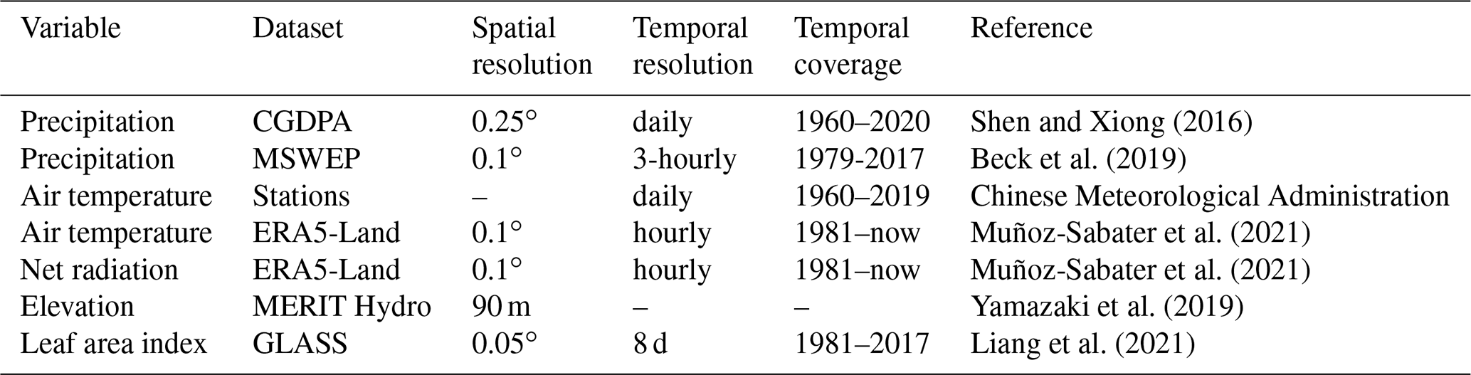
Information about the forcing data and auxiliary data is listed in Table 1. These data are the input of the reconstruction methods, i.e., machine learning modeling and hydrological modeling. Precipitation data include the China Gauge-based Daily Precipitation Analysis (CGDPA; Shen and Xiong, 2016) and the Multi-Source Weighted-Ensemble Precipitation (MSWEP version 2.2; Beck et al., 2019). The daily 0.25∘ CGDPA data are produced using a spatial interpolation of observations from approximately 2400 ground rain gauge stations. The 3-hourly 0.1∘ MSWEP data are produced by optimally merging a range of gauge station, satellite, and reanalysis datasets. In addition to precipitation data, hydrological modeling requires air temperature (T) and net radiation data (Rn) as forcing data. Air temperature data include the observations from approximately 2400 ground stations provided by the Chinese Meteorological Administration and ERA5-Land 2 m temperature (Muñoz-Sabater et al., 2021). Note that the number of available ground stations for T was around 800 before 1988. Net radiation data are from ERA5-Land (Muñoz-Sabater et al., 2021). Elevation (Elev) data are from MERIT Hydro (Yamazaki et al., 2019). Leaf area index (LAI) data are from the Global Land Surface Satellite (GLASS; Liang et al., 2021) dataset.
2.2 Validation data
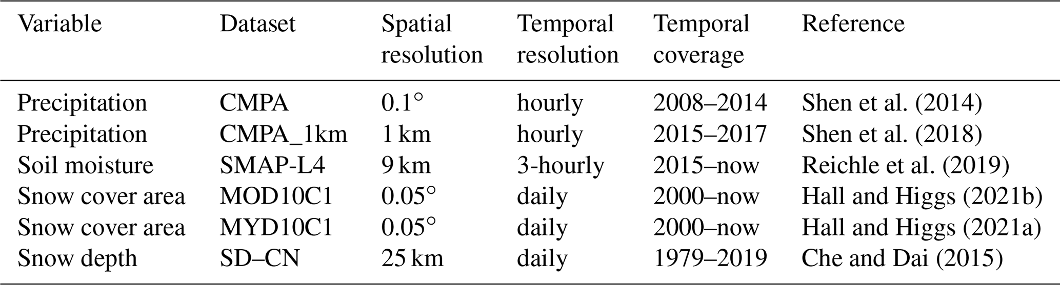
Information about the validation data is listed in Table 2. The validation data are the reconstruction targets of the study, and therefore they are also used for model training (for precipitation) and calibration (for soil moisture and snow water equivalent). Details about validation methods are introduced in Sect. 3. All following satellite-based data provide direct or indirect measurements of the variables to be reconstructed over a large spatial extent. P data include the China Merged Precipitation Analysis (CMPA; Shen et al., 2014) and its successor, the CMPA_1km (Shen et al., 2018). The CMPA has merged more than 30 000 automatic weather stations with the Climate Precipitation Center Morphing (CMORPH; Joyce et al., 2004) product to produce an hourly 0.1∘ dataset from 2008. Starting from 2015, the CMPA_1km upgrades the CMPA by using more than 40 000 automatic weather stations and adding radar P estimations in the merging procedure, which increases the spatial resolution to 1 km. In this study, the CMPA_1km was spatially aggregated into 0.1∘ to extend the time span of the CMPA data. The CMPA refers to the combination of the CMPA and CMPA_1km in the following part of the paper. Note that precipitation data during the cold season (from October to April) in northern and western China are mainly derived from remote sensing data, since automatic weather stations do not operate under low temperatures (Shen et al., 2014, 2018). SM data are obtained from the Soil Moisture Active Passive Mission Level 4 (SMAP-L4; Reichle et al., 2019) data. SMAP-L4 assimilates SMAP radiometer brightness temperature into the NASA catchment land surface model to produce a 3-hourly 9 km volumetric SM dataset in the root zone (0–100 cm). Since there is no direct measurement of SWE, we use snow cover areas and snow depths as surrogates. Snow cover area (SCA) data are obtained from MOD10C1 (Hall and Higgs, 2021b) and MYD10C1 (Hall and Higgs, 2021a), which collect snow extent information from the Moderate-Resolution Imaging Spectroradiometer (MODIS) sensors from Terra and Aqua platforms respectively. Compiled at daily and 0.05∘ scales, MOD10C1 and MYD10C1 provide snow cover percentage and cloud cover percentage at each grid. Snow depth data are obtained from the long-term series of daily snow depth datasets in China (SD–CN; Che and Dai, 2015). The 25 km daily snow depth of SD–CN is derived from the passive microwave brightness temperature from SMMR, SSM/I, and SSMI/S sensors. Although SD–CN is long enough for many hydrological studies, it is limited by a coarse spatial resolution.
The workflow of the study is presented in Fig. 1. Firstly, we reconstruct the precipitation data, and then we use the reconstructed precipitation as forcing input to reconstruct soil moisture and snow water equivalent.

Figure 1Workflow of the study. P: precipitation, Elev: elevation, LAI: leaf area index, T: air temperature, Rn: net radiation, PET: potential evaporation, SWE: snow water equivalent, SCA: snow cover area, SM: soil moisture, Rain: liquid rainfall, Snow: snowfall, Melt: snowmelt, RF: random forest, LR: linear regression.
3.1 Reconstruction of precipitation
We applied machine learning to predict the CMPA precipitation grid by grid using grid coordinates, P from the CGDPA and MSWEP and Elev and LAI as input. All data were preprocessed to be daily and 0.1∘ under the WGS 84 latitude–longitude coordinate system (EPSG:4326). The MSWEP P and CMPA P were aggregated to be daily. GLASS LAI was set to be the same within the 8 d of an 8 d composite. The MERIT Hydro Elev data were spatially aggregated into 0.1∘. The CGDPA P data were resampled into 0.1∘ using bilinear interpolation. The difference between the ground-truth 0.1∘P and the resampled 0.1∘P from the CGDPA is spatially correlated with the sub-grid distribution of Elev and LAI in a 0.25∘ grid. Therefore, we created two new input features, Elevdiff and LAIdiff, to account for the differences between the true 0.1∘ value and the value resampled from a 0.25∘ resolution for Elev and LAI. Specifically, Elev and LAI were aggregated into 0.25∘, resampled into 0.1∘ using bilinear interpolation, and then subtracted by the original 0.1∘ layer.
The training strategy is presented in Fig. 2. We divided the model training into two parts: a binary classification problem that predicted whether the grid was rainy (P > 0 mm) and a regression problem which predicted the value of P in rainy grids. We proposed a tile-by-tile training strategy that fits a machine learning model with all samples of one hundred 0.1∘ grids in a 1∘ tile. To be specific, although the target PCMPA in a 0.1∘ grid was predicted by grid coordinates, as well as PCGDPA, PMSWEP, Elev, Elevdiff, LAI, and LAIdiff in the same grid, all grids in the same 1∘ tile shared a common prediction model. This tile-by-tile training strategy increased the size of samples and made use of the spatial information of Elev and LAI. Since the CMPA data were not reliable during the cold season in northern and western China because of lacking ground-based observations, we discarded training samples from October to April in two regions (Shen et al., 2018): (1) latitude > 40∘ N and (2) 40∘ N > latitude > 27∘ N and longitude < 100∘ E.
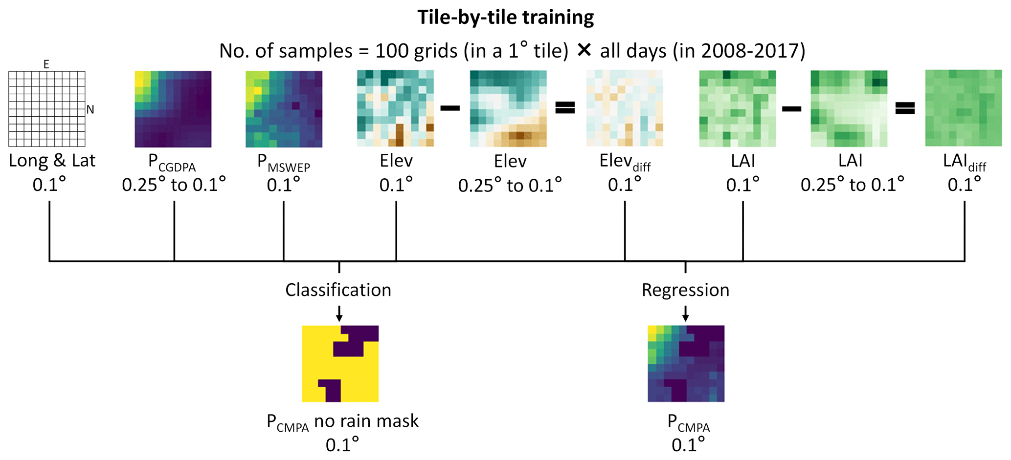
Figure 2Model training strategies of precipitation reconstruction. P: precipitation, Elev: elevation, LAI: leaf area index.
The machine learning model for the rain/no rain classification is the random forest (Breiman, 2001). The model for the P regression is a neural network (Foresee and Hagan, 1997) that stacks a linear regression model and a random forest model, as shown in Fig. 3. Stacking (Wolpert, 1992) is a model ensemble method that optimally combines multiple base machine learning models for predictions. In the stacking process, all base models are first trained to get out-of-bag predictions in the cross-validation, and then a stacking model is trained using the out-of-bag predictions of the base models as input. The random forest model can deal with non-linear relationships and complex interactions among input features. The linear model can extrapolate the predictions that are out of the range of training samples. A stacking model leveraged the advantages of these two base models. We chose 5-fold cross-validation for hyper-parameter tuning and performance evaluation in both the classification and regression problems. All folds were created by the spatial and temporal mixed splitting of the data samples. Specifically, we put the data of one hundred 0.1∘ grids in a 1∘ tile on all days together to form a training dataset and then randomly split it into 5 folds. Each sample corresponded to the data of one 0.1∘ grid on 1 d. After the model training, we used the data of PCGDPA and PMSWEP from 1981–2017 combined with grid coordinates, Elev, Elevdiff, LAI, and LAIdiff, to predict PCMPA in the same period, which produced a consistent long-term reconstructed dataset, PRec, as shown in Fig. 1. Note that we only predicted P values on rainy days according to the classification model during the reconstruction.

Validation metrics include two classification metrics, i.e., probability of detection (POD) and false alarm rate (FAR), as well as two regression metrics, i.e., Kling–Gupta efficiency (KGE) and normalized root mean square error (NRMSE). Equations of the metrics are listed in Eqs. (1) to (4):
where n11 is the number of actual rainy days that are predicted to be rainy, n01 is the number of actual rainy days that are predicted to have no rain, n10 is the opposite of n01, r is the correlation between predicted and target P, μO and μS are the mean values of target and predicted P respectively, σO and σS are the standard deviations of target and predicted P respectively, Si is the predicted value of P on the ith rainy day, and Oi is the target value of P on the ith rainy day. The perfect values are 1 for POD and KGE and 0 for FAR and NRMSE. Note that the predictions are validated in 5-fold cross-validation of the model. For grids in northern (latitude > 40∘ N) and western (40∘ N > latitude > 27∘ N and longitude < 100∘ E) China, only predictions in May–September are validated.
3.2 Reconstruction of soil moisture and snow water equivalent
We used the modified HBV hydrological model (Bergström, 1992; Parajka et al., 2007) calibrated by satellite-based data grid by grid to reconstruct SWE and SM. The HBV model has low computational complexity and general applicability in various climate conditions (Beck et al., 2020; Seibert and Bergström, 2022) and shows a high capability of simulating soil moisture in various regions of the world (Beck et al., 2021). Note that we added a canopy interception module (Mao and Liu, 2019) to the traditional HBV model, as presented in Fig. 4. The HBV model is calibrated at a 0.1∘ resolution under the WGS 84 latitude–longitude coordinate system (EPSG:4326). The forcing input of the model includes P, T, and potential evaporation (PET). The reconstructed P was regarded as the precipitation input. The 0.1∘T was created by the interpolation of observations from ground stations using co-kriging (Myers, 1982) with Elev and the daily-aggregated ERA5-Land T as covariates. PET was calculated using the Priestley–Taylor equation (Priestley and Taylor, 1972) with interpolated T and daily-aggregated ERA5-Land Rn.
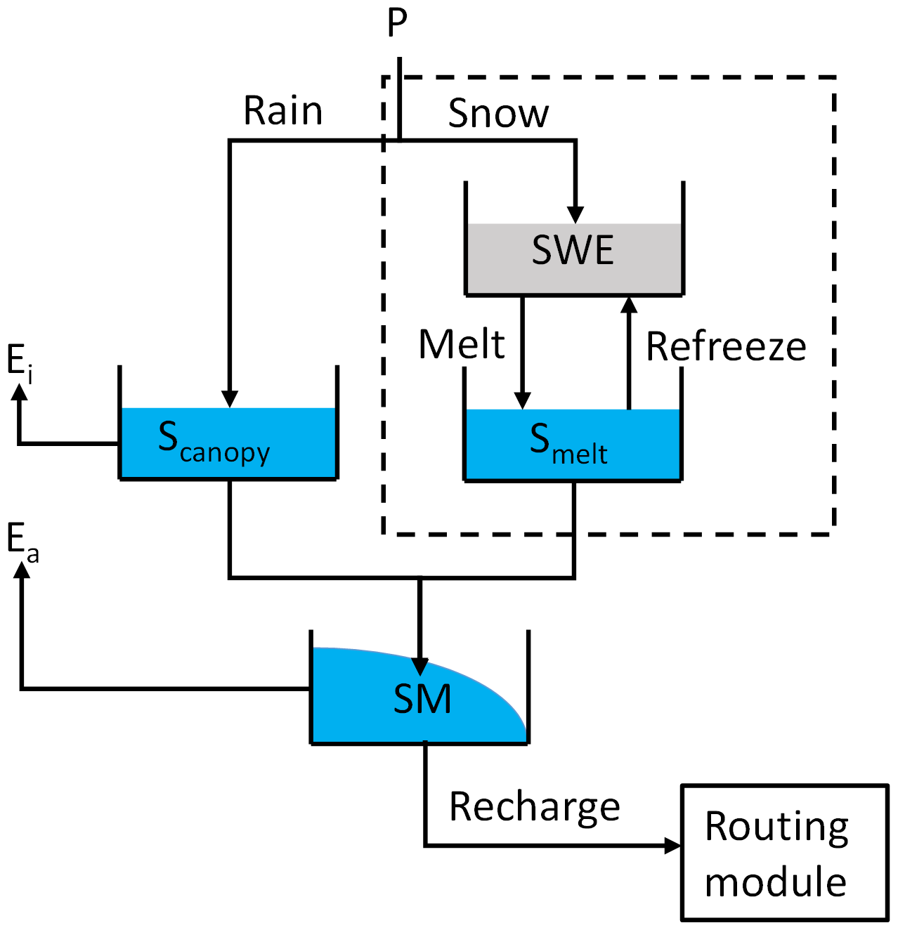
Figure 4Illustration of the HBV model used for the reconstruction of soil moisture and snow water equivalent. The dashed box illustrates the snow module.
The calibration targets SCA, SWE, and SM were preprocessed from the raw data in Table 2. The 0.05∘ SCA data from MOD10C1 or MYD10C1 were first aggregated to be 0.1∘. Then, for each grid, we extracted all days in November–April when the cloud cover percentages were smaller than 40 % and calculated the percentage of snow extent in the no cloud fraction of the grid to get the final SCA. The calibration of SCA was converted to a binary classification problem where the SCA from MOD10C1 or MYD10C1 was set to 1 if SCA > 10 % otherwise 0. In the HBV model, SCA was calculated by the binarization of SWE, which meant SCA = 1 if SWE exceeded a snowpack threshold Tcover otherwise SCA = 0. For SWE, we first resampled the 25 km snow depth from SD–CN into 0.1∘ using bilinear interpolation. Then, the SWE was calculated by multiplying snow depth and snow density. We used a fixed value of snow density at a national scale, 0.18 g cm−3, which was reasonable for most snow-affected areas in China (Yang et al., 2019; Gao et al., 2020; Yang et al., 2020a). For SM, the 1 m root zone SM from SMAP-L4 was resampled from 9 km to 0.1∘ using bilinear interpolation and aggregated from 3 h to 1 d.
For each grid, we first calibrated the parameters of the snow module and then calibrated the soil water module with the optimal snow module parameters. This two-step calibration strategy alleviated parameter equifinality, since two modules were calibrated separately. The snow module was only calibrated in grids where at least 5 % of days had T < 0 ∘C. All parameters to be calibrated are presented in Table 3. After calibration, we used the historical PRec, PET, T, and LAI to drive the HBV model to simulate long-term rainfall (RainRec), snowfall (SnowRec), snow water equivalent (SWERec), snowmelt (MeltRec), and soil moisture (SMRec), as shown in Fig. 1.
Table 3Parameters of the HBV model and their ranges for model calibration.

The validation metric for SCA is balanced accuracy (BACC):
where n11 is the number of snow cover days that are predicted to have snow cover, n00 is the number of no snow cover days that are predicted to have no snow cover, n01 is the number of snow cover days that are predicted to have no snow cover, and n10 is the opposite of n01.
The validation metric for SWE and SM is KGE in Eq. (3), where r is the correlation between predicted and target SWE or SM, σO and σS are the standard deviations of target and predicted SWE or SM respectively, and μO and μS are the mean values of target and predicted SWE or SM respectively. During the calibration, the optimization target of the snow module was 1–14 × BACC − 34 × KGE, which optimized the simulation performances of SCA and SWE at the same time. With small numbers of model parameters, the parsimonious snow and soil water modules were unlikely to overfit the target data. Therefore, we validated the performance of the reconstruction using the performance of the calibration directly.
4.1 Validation of precipitation
Table 4 summarizes the performance of different P datasets in all grids benchmarked by PCMPA. For rain/no rain classification, the reconstructed P (PRec) achieves a balance of the POD and FAR. The median POD of PRec is 0.87, which is slightly worse than PCGDPA (POD = 0.92) and far better than PMSWEP (POD = 0.74). The median FAR of PRec is 0.19, which is better than PCGDPA (FAR = 0.23) but slightly worse than PMSWEP (FAR = 0.18). Since the 0.1∘PCGDPA is resampled from the 0.25∘ dataset, it certainly overestimates the probability of rain and has a high POD and FAR at the same time naturally. On the opposite side, with the finer spatial information from satellite data, PMSWEP is skilled in detecting no-rain days, and thus it tends to have better FAR performance. In summary, PRec improves the FAR of PCGDPA without scarifying too many POD. For P regression, PRec outperforms PCGDPA and PMSWEP significantly. The median KGEs of PRec, PCGDPA, and PMSWEP are 0.68, 0.51, and 0.53 respectively, and the median NRMSEs of PRec, PCGDPA, and PMSWEP are 0.63, 0.91, and 0.82 respectively.
Table 4Validation of the reconstructed precipitation in all grids at a national scale. The benchmark dataset is the CMPA. POD: probability of detection, FAR: false alarm rate, KGE: Kling–Gupta efficiency, NRMSE: normalized root mean squared error. In northern (latitude > 40∘ N) and western (40∘ N > latitude > 27∘ N and longitude < 100∘ E) China, only data in May–September are used for validation.
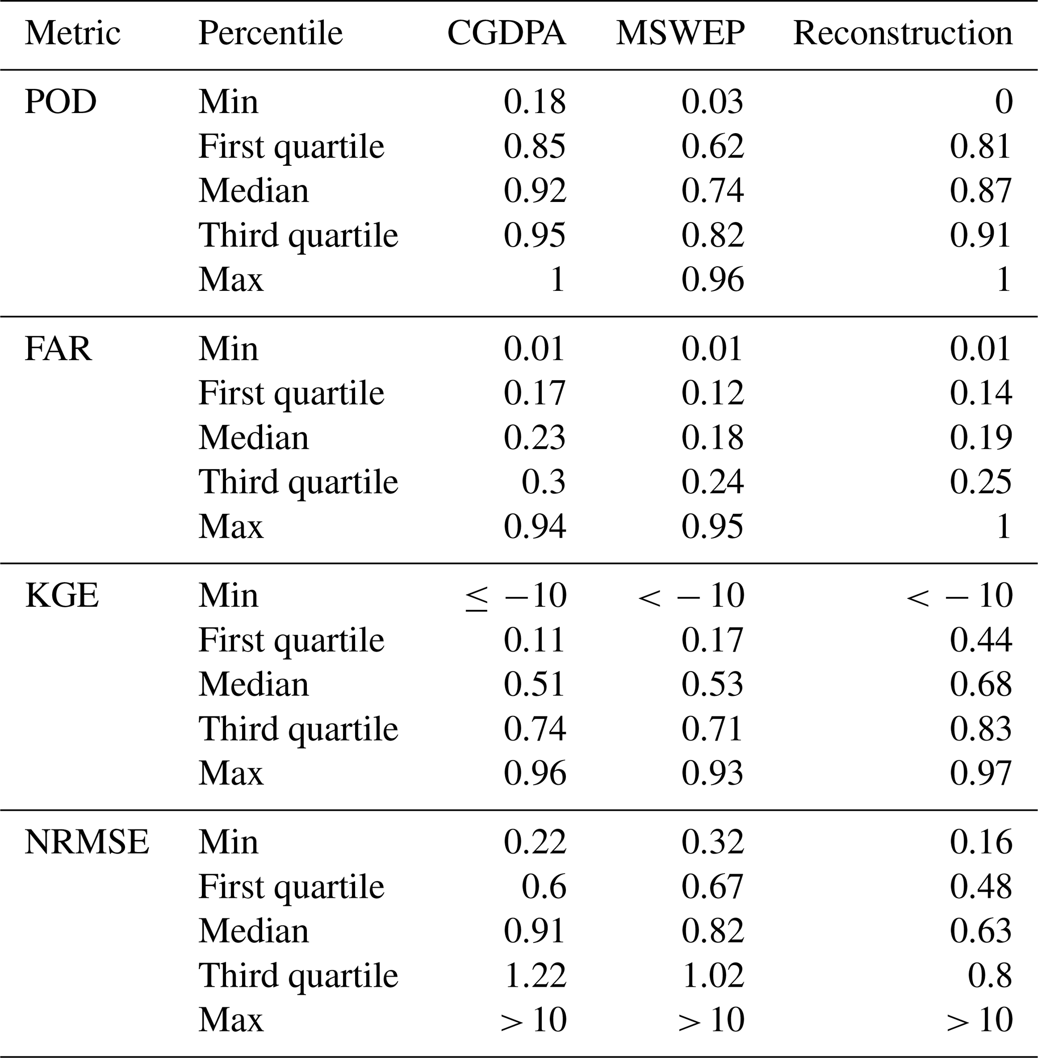
Table 5 presents the median values of all metrics for PRec in nine major basins of China. Figure 5 presents the spatial distribution of validation metrics for PRec and the metric differences between PRec and PCGDPA, as well as PRec and PMSWEP. For rain/no rain classification, PRec performs well since the median POD > 0.83 and FAR < 0.22 for all major basins except for the southwest basin, according to Table 5. According to Fig. 5a and d, the best performance occurs in the driest part of the northwest continental basin where rain is rare, and the worst performance occurs in the plateau such as the upper stream areas of the Yangtze River basin and the southwest basin. The balance of POD and FAR can be seen in Fig. 5b, c, e, and f, where PRec trades POD for FAR compared with PCGDPA and trades FAR for POD compared with PMSWEP. For P regression, in addition to the northwest continental basin and the upper stream of the southwest basin where the coverage of ground stations is low (Shen et al., 2014, 2018), all other major basins have median KGEs over 0.76 and NRMSEs under 0.55, which indicates good performance, according to Table 5. According to Fig. 5g and j, with KGE > 0.8 and NRMSE < 0.5 in a majority of grids, PRec is very accurate in a large part of the eastern region, probably because of the dense distribution of ground stations for the CGDPA (Shen and Xiong, 2016). According to Fig. 5h, i, k, and l, PRec outperforms PCGDPA and PMSWEP almost in the whole country. PRec improves PCGDPA and PMSWEP the most in the northwest continental basin and the upper stream of the southwest basin where the distribution of ground stations is sparse, even though the performance of PRec is still limited in this area.
Table 5Validation of the reconstructed precipitation in nine major basins of China. The benchmark dataset is the CMPA. POD: probability of detection, FAR: false alarm rate, KGE: Kling–Gupta efficiency, NRMSE: normalized root mean squared error. In northern (latitude > 40∘ N) and western (40∘ N > latitude > 27∘ N and longitude < 100∘ E) China, only data in May–September are used for validation.
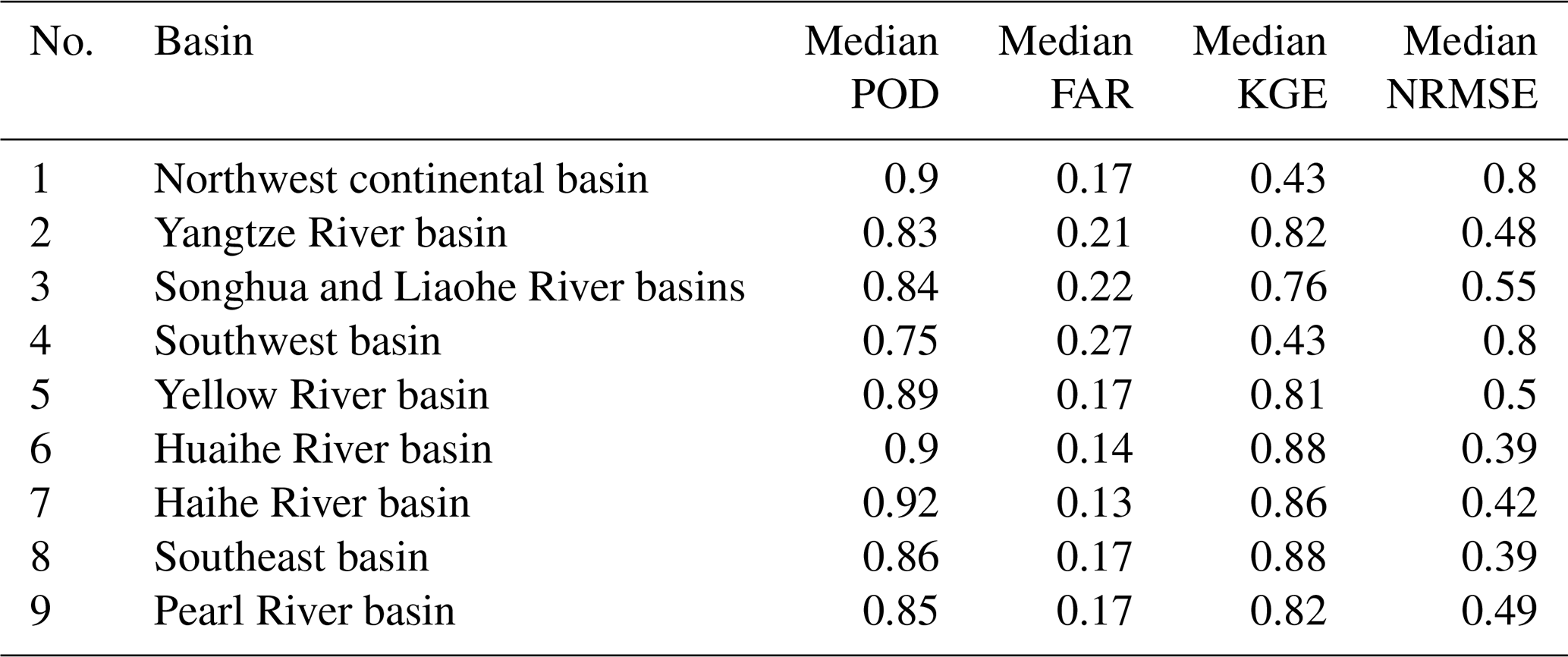
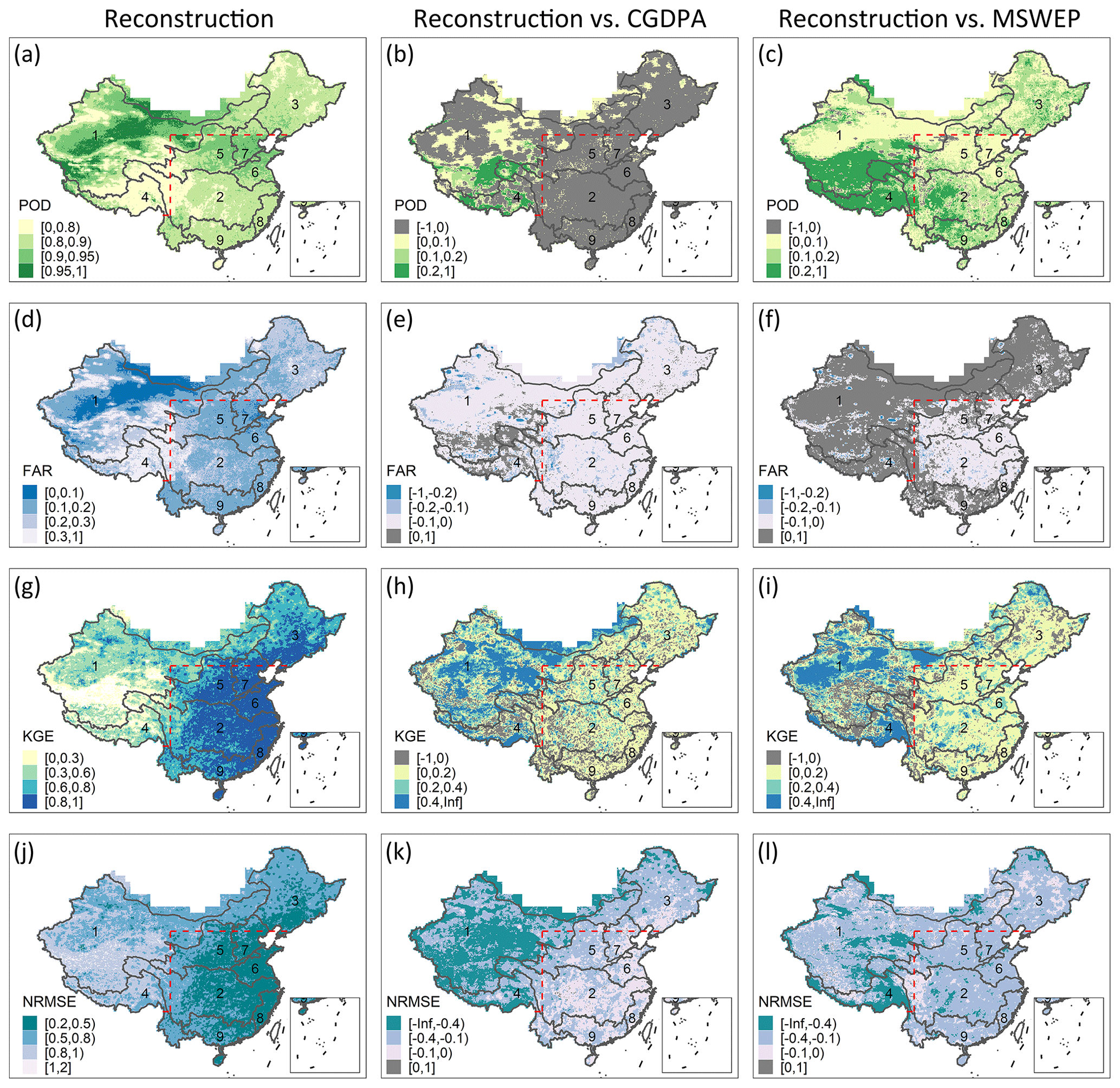
Figure 5Spatial validation of the reconstructed precipitation. The benchmark dataset is the CMPA. POD: probability of detection, FAR: false alarm rate, KGE: Kling–Gupta efficiency, NRMSE: normalized root mean squared error. The second and third columns are the differences of validated metrics between the reconstructed dataset and the CGDPA and MSWEP datasets. The boundary lines delineate nine major river basins of China: (1) the northwest continental basin, (2) the Yangtze River basin, (3) the Songhua and Liaohe River basins, (4) the southwest basin, (5) the Yellow River basin, (6) the Huaihe River basin, (7) the Haihe River basin, (8) the southeast basin, and (9) the Pearl River basin. In northern (latitude > 40∘ N) and western (40∘ N > latitude > 27∘ N and longitude < 100∘ E) China above the dashed lines, only data in May–September are validated.
Figure 6 presents the spatial distribution of annual average P and the time series of monthly P for PCMPA and PRec. PRec matches PCMPA well, both spatially and temporally, for nine major basins at a large temporal scale. According to Fig. 6a, PRec does not smooth the spatial distribution of P, which indicates that the tile-by-tile training strategy learns the local variations of P within the tile. Except for the northwest continental basin and the Songhua and Liaohe River basins where the cold season precipitation data are not reliable for the CMPA, all other basins have KGE values larger than 0.91 for monthly time series, according to Fig. 6b.
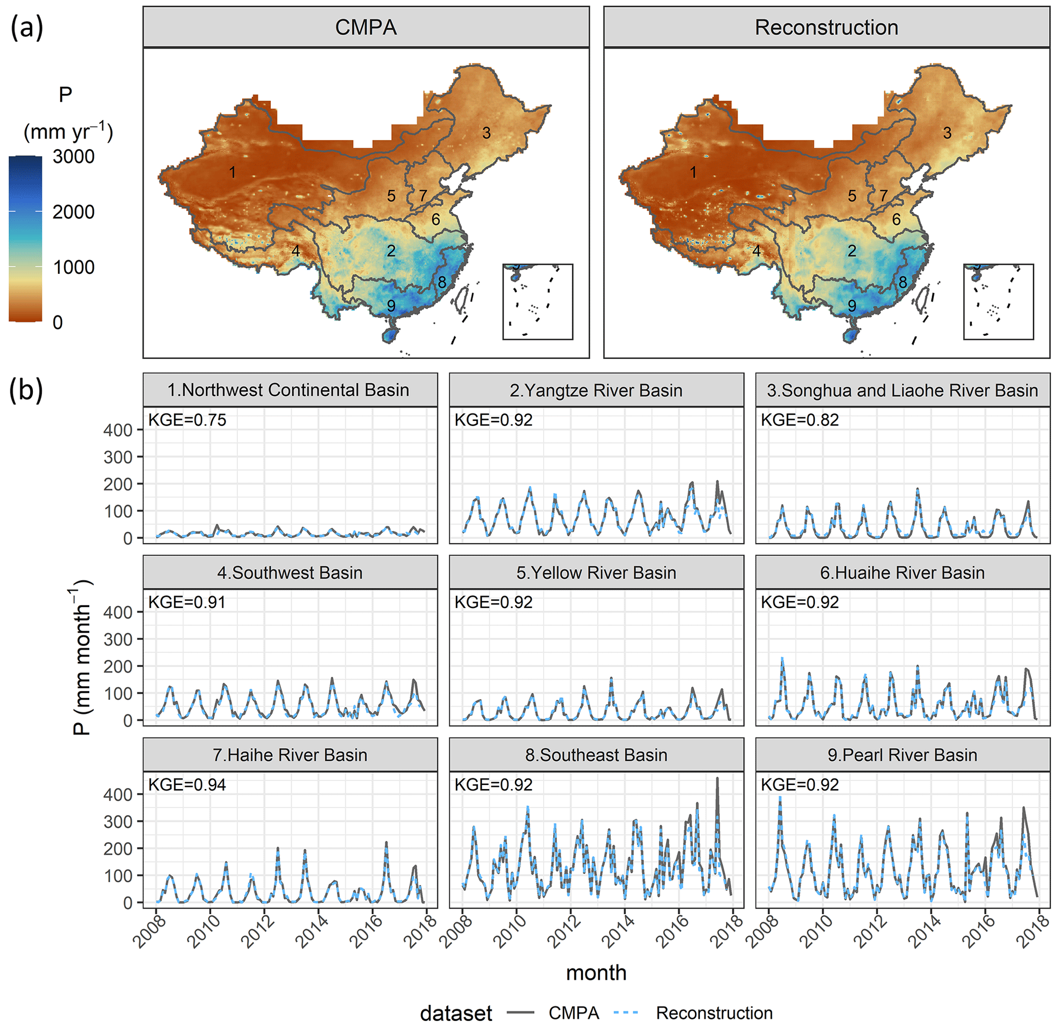
Figure 6(a) Map of the annual average precipitation (P) of the CMPA and reconstruction in 2008–2017. (b) Time series of the monthly P of the CMPA and reconstruction for nine major river basins in 2008–2017. Note that the CMPA has missing values in 2015; we only choose the days when the CMPA has available data in the temporal aggregation for both the CMPA and reconstruction. Here the reconstructed P data are out-of-bag predictions in the cross-validation.
4.2 Validation of soil moisture and snow water equivalent
Table 6 summarizes the performance of reconstructed SWERec, SCARec, and SMRec in all grids. While the snow module of the HBV model performs poorly with the median KGE = −0.31 for SWERec at a national scale, it has certain skills in simulating snow cover with the median BACC = 0.65 for SCARec. The soil water module of the HBV model performs well with the median KGE = 0.61 for SMRec.
Table 6Validation of the reconstructed snow water equivalent (SWE), snow cover area (SCA), and soil moisture (SM) in all grids at a national scale. The benchmark datasets are SD–CN for SWE, MOD10C1/MYD10C1 for SCA, and SMAP-L4 for SM. KGE: Kling–Gupta efficiency, BACC: balanced accuracy.
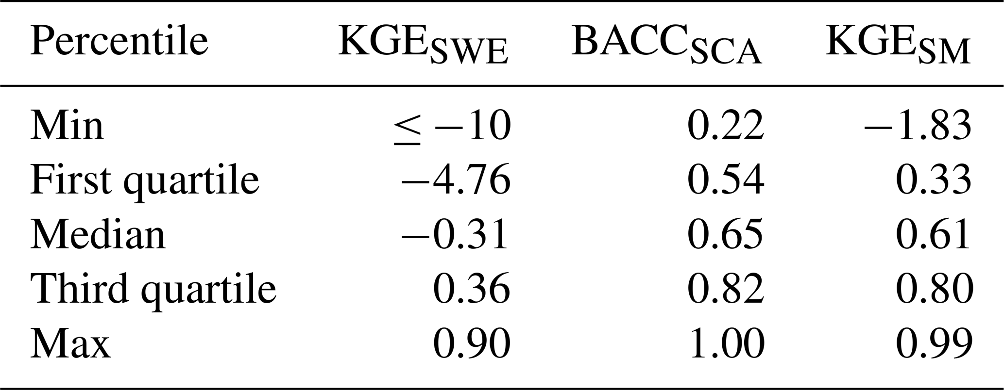
Table 7Validation of the reconstructed snow water equivalent (SWE) and snow cover area (SCA) in nine major basins of China. The benchmark datasets are SD–CN for SWE, MOD10C1/MYD10C1 for SCA, and SMAP-L4 for SM. KGE: Kling–Gupta efficiency, BACC: balanced accuracy.
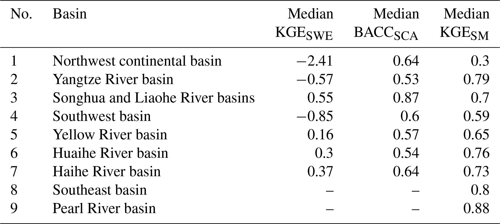
Table 7 presents the median values of all metrics for SWERec, SCARec, and SMRec in nine major basins of China. Figure 7 presents the spatial distribution of validation metrics for SWERec, SCARec, and SMRec. The performance of snow reconstruction varies spatially. There are three major snow cover areas in China: northeastern China, northern Xinjiang, and the Tibetan Plateau. According to Fig. 7a and b, SWERec and SCARec perform well in both northeast China and northern Xinjiang with KGESWE > 0.7 and BACCSCA > 0.8 in many grids, while SWERec and SCARec perform poorly with KGESWE < 0 and BACCSCA < 0.5 in a large part of the Tibetan Plateau, where snow-driven hydrological processes are complex (Gao et al., 2020). According to Table 7, SWERec and SCARec perform the best in the Songhua and Liaohe River basins (i.e., northeast China) with KGESWE= 0.55 and BACCSCA= 0.87, where snowmelt contributes a considerable amount of water to runoff and floods (Qi et al., 2021). The performance of soil moisture reconstruction also varies spatially. According to Fig. 7c, SMRec performs well in a large part of southern China. However, in the northwest continental basin where the climate is dryer and the topography is more complex, SMRec performs relatively poorly with median KGESM= 0.3. Generally, SMRec performs better in southern basins, e.g., the Yangtze River basin, the Huaihe River basin, the southeast basin, and the Pearl River basin, where the values of median KGESM are at least 0.76, according to Table 7. Note that the accuracy of SWERec, SCARec, and SMRec in different areas may depend on the quality of the benchmark datasets and the ability of the HBV model to represent local hydrological processes.
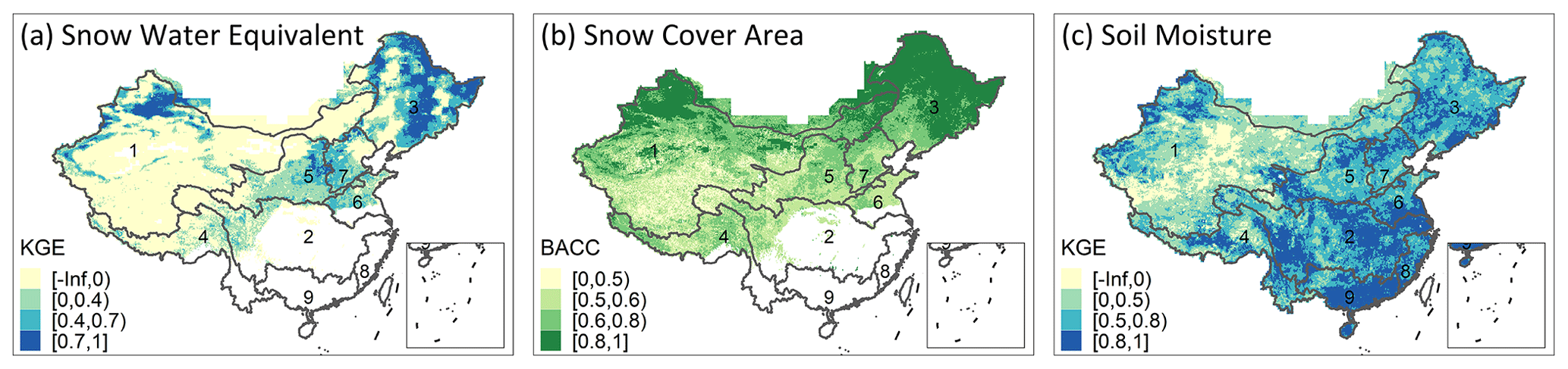
Figure 7Spatial validation of the reconstructed snow water equivalent (SWE), snow cover area (SCA), and soil moisture (SM). The benchmark datasets are SD–CN for SWE, MOD10C1/MYD10C1 for SCA, and SMAP-L4 for SM. KGE: Kling–Gupta efficiency, BACC: balanced accuracy. The boundary lines delineate nine major river basins of China: (1) the northwest continental basin, (2) the Yangtze River basin, (3) the Songhua and Liaohe River basins, (4) the southwest basin, (5) the Yellow River basin, (6) the Huaihe River basin, (7) the Haihe River basin, (8) the southeast basin, and (9) the Pearl River basin.
Figure 8 presents the spatial distribution of daily average SWE and the time series of daily average SWE for SWESD–CN and SWERec in each month. Figure 8a shows that SWERec successfully detects areas with large SWE. Figure 8b shows that, although SWERec captures the temporal variations of SWE in all basins, it overestimates the magnitudes of SWE in the northwest continental basin, the Yangtze River basin, the southwest basin, and the Yellow River basin. In the Songhua and Liaohe River basins with KGE = 0.68 and the Haihe River basin with KGE = 0.46, SWERec can accurately capture both the temporal variations and the magnitudes of SWE. The magnitudes of SWE are difficult to simulate for three reasons. First, SWESD–CN is an estimation of SWE from the multiplication of snow depth and a fixed snow density; second, the original spatial resolution of SWESD–CN is 25 km, which may be too coarse to represent snow distribution, especially in mountain regions; third, the new reconstructed precipitation dataset may not capture snowfall well. Figure 9 presents the spatial distribution of daily average SM and the time series of daily average SM for SMSMAP-L4 and SMRec in each month. SMRec captures the spatial and temporal variations of SMSMAP-L4 well except in the northwest continental basin. Although the monthly KGE values in all basins are larger than 0.59 except for the northwest continental basin, SMRec slightly underestimates SMSMAP-L4 at a monthly scale in all basins.
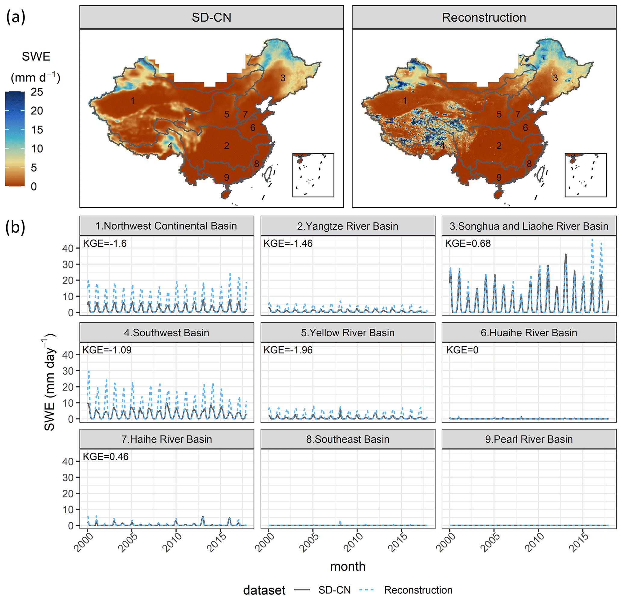
Figure 8(a) Map of daily average snow water equivalent (SWE) of SD–CN and reconstruction in 2000–2017. (b) Time series of the daily average SWE of SD–CN and reconstruction for nine major river basins in each month of 2000–2017.
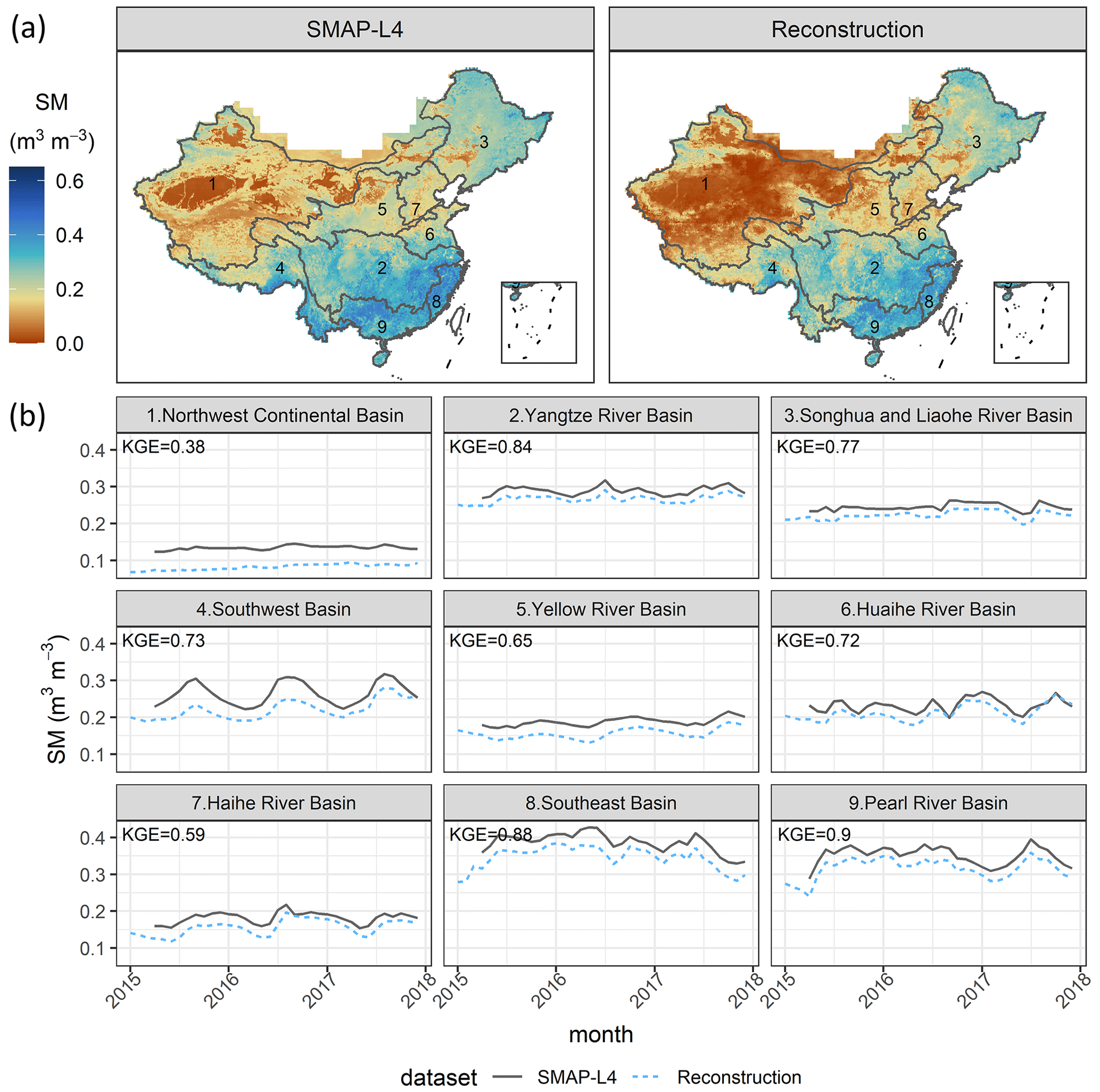
Figure 9(a) Map of daily average soil moisture (SM) of SMAP-L4 and reconstruction in 2015–2017. (b) Time series of the daily average SM of SMAP-L4 and reconstruction for nine major river basins in each month of 2015–2017.
4.3 Limitations of the reconstruction dataset
Uncertainties of the reconstruction dataset come from the quality of the input data and the limitations of the reconstruction models. For precipitation, although the benchmarked dataset CMPA includes satellite information to produce P data, it still has large errors in western China due to the small number of automatic weather stations for local corrections in this area. Another problem of the CMPA data is the possible inconsistency between the CMPA and its successor, the CMPA_1km. Although the main observation sources and the deriving method are similar, the discrepancy between the CMPA and CMPA_1km has not been investigated in previous studies. Combining the CMPA and CMPA_1km trades consistency for more data samples in machine learning algorithms. In addition, the quality of MSWEP is not consistent over time, since the available data sources to be merged are changing in different periods. Furthermore, although the stacking machine learning model can extrapolate, it may have problems in reconstructing extreme P values, since the extrapolation relies on a linear regression model, which may fail to capture the complex relationship between the target P and input variables. For snow water equivalent, a unified snow density (0.18 g cm−3) may cause a large bias in estimating SWE in some regions. The coarse resolution of the benchmarked SWE is also a major concern: although the MODIS SCA data add sub-grid information to the 0.25∘ SD–CN data, we still do not have a benchmarked SWE dataset that is originally 0.1∘. Another limitation is the unknown applicability of the HBV model at a national scale. HBV uses a temperature-based snow module without an energy balance component or a glacier module, which may fail in areas with more complex snow processes such as the Tibetan Plateau (Gao et al., 2020). For soil moisture, the benchmarked SMAP-L4 is an assimilated dataset without actual measurements of root zone SM. In addition, PET is calculated without local Rn data. The uncertainty of PET may propagate to SM. Moreover, it is unclear whether HBV is suitable for soil water simulation at a national scale in China.
Reconstruction data do not have better accuracy than the satellite-based benchmark data we used. Instead, reconstruction aims to extend the state-of-the-art satellite-based data of P, SM, and SWE to the 1980s in China. Therefore, the value of the reconstruction data is to support hydrological studies focusing on a longer time span (e.g., 30 years) rather than recent years.
We created a long-term (1981–2017) 0.1∘ daily dataset of total precipitation (P), liquid rainfall (Rain), snowfall (Snow), snow water equivalent (SWE), snowmelt (Melt), and soil moisture (SM) in China by reconstructing high-resolution satellite-based data. P was reconstructed by predicting the CMPA data from the CGDPA and MSWEP data using a stacking machine learning model. Other variables were simulated by the HBV model with SWE calibrated by SD–CN, SCA calibrated by MOD10C1/MYD10C1, and SM calibrated by SMAP-L4. Evaluations of the reconstruction data are as follows.
Benchmarked by the CMPA at a national scale, the median POD and FAR of the reconstructed P are 0.87 and 0.19 respectively for rain/no rain classification, and the median KGE and NRMSE of the reconstructed P are 0.68 and 0.63 respectively for P regression on rainy days. The reconstructed P improves the CGDPA and MSWEP data, whose median KGEs are 0.51 and 0.53. The median KGEs are smaller than 0.43 in the northwest continental basin and the southwest basin and larger than 0.76 in other major basins. At a monthly scale, all basins have KGE values larger than 0.91 except for the northwest continental basin and the Songhua and Liaohe River basins, where the benchmarked precipitation data in cold seasons are not reliable.
Benchmarked by SD–CN and MOD10C1/MYD10C1 at a national scale, the median KGE of the reconstructed SWE and the median BACC of the reconstructed SCA are −0.31 and 0.65 respectively. The reconstructed SWE performs the best in the Songhua and Liaohe River basins with KGE = 0.55 but performs the worst in the northwest continental basin where the median KGE is −2.41. At a monthly scale, the reconstructed SWE captures the monthly variability of the SWE derived from SD–CN in all basins. However, the reconstructed SWE only reproduces SWE magnitudes accurately in the Songhua and Liaohe River basins (monthly KGE = 0.68) and the Haihe River basin (monthly KGE = 0.46) but overestimates the SWE magnitudes in other basins.
Benchmarked by SMAP-L4 at a national scale, the median KGE of the reconstructed SM is 0.61. SMRec performs well in southern basins, e.g., the Yangtze River basin, the Huaihe River basin, the southeast basin, and the Pearl River basin, where the values of median KGESM are at least 0.76. SMRec performs the worst in the northwest continental basin where the median KGESM= 0.3. At a monthly scale, the KGE values in all basins are larger than 0.59 except in the northwest continental basin.
This study is the first attempt to produce a long-term (at least 30 years) 0.1∘ daily dataset of P, SM, and SWE that combines high-accuracy local information and high-resolution satellite-based data via reconstruction. This dataset is especially suitable for exploring the relationship between riverine streamflow and hydrological drivers, since the P, SM, and SWE are produced independently from streamflow data. Future improvements include extending the temporal length of the dataset and formulating a model strategy that handles the spatial variability of the hydrological processes at a national scale.
The source codes for model training, model calibration, and data reconstruction are available at https://doi.org/10.5281/zenodo.7450278 (Yang, 2022).
The reconstruction datasets of total precipitation, rainfall, snowfall, snow water equivalent, snowmelt, and soil moisture are freely available at https://doi.org/10.5281/zenodo.5811099 (Yang et al., 2021).
WY and HY conceptualized the study. WY developed the methodology, performed the analysis, and wrote the original draft of the paper. All other authors contributed to the review and revision of the paper. HY, QH, and DY helped with the data collection. HY and DY were responsible for funding acquisition.
The contact author has declared that none of the authors has any competing interests.
Publisher's note: Copernicus Publications remains neutral with regard to jurisdictional claims in published maps and institutional affiliations.
We thank the China Meteorological Administration for providing national precipitation data (the CGDPA, CMPA, and CMPA_1km) and air temperature data from meteorological stations.
This research was supported by the China National Key R&D Program (grant no. 2021YFC3000202), the National Natural Science Foundation of China (grant nos. 51979140, 42041004), the State Key Laboratory of Hydro Science and Hydraulic Engineering of China (grant no. 2021-KY-04), and the Key Research and Development Program of Yunnan Province, China (grant no. 202203AA080010).
This paper was edited by Yue-Ping Xu and reviewed by two anonymous referees.
Abelen, S., Seitz, F., Abarca-del-Rio, R., and Guntner, A.: Droughts and Floods in the La Plata Basin in Soil Moisture Data and GRACE, Remote Sens.-Basel, 7, 7324–7349, https://doi.org/10.3390/rs70607324, 2015.
Beck, H. E., Wood, E. F., Pan, M., Fisher, C. K., Miralles, D. G., van Dijk, A. I. J. M., McVicar, T. R., and Adler, R. F.: MSWEP V2 Global 3-Hourly 0.1 degrees Precipitation: Methodology and Quantitative Assessment, B. Am. Meteorol. Soc., 100, 473–502, https://doi.org/10.1175/Bams-D-17-0138.1, 2019.
Beck, H. E., Pan, M., Lin, P., Seibert, J., van Dijk, A. I., and Wood, E. F.: Global fully distributed parameter regionalization based on observed streamflow from 4,229 headwater catchments, J. Geophys. Res.-Atmos., 125, e2019JD031485, https://doi.org/10.1029/2019jd031485, 2020.
Beck, H. E., Pan, M., Miralles, D. G., Reichle, R. H., Dorigo, W. A., Hahn, S., Sheffield, J., Karthikeyan, L., Balsamo, G., Parinussa, R. M., van Dijk, A. I. J. M., Du, J., Kimball, J. S., Vergopolan, N., and Wood, E. F.: Evaluation of 18 satellite- and model-based soil moisture products using in situ measurements from 826 sensors, Hydrol. Earth Syst. Sci., 25, 17–40, https://doi.org/10.5194/hess-25-17-2021, 2021.
Bergström, S.: The HBV model – its structure and applications, SMHI Reports RH 4, Swedish Meteorological and Hydrological Institute (SMHI), Norrköping, Sweden, https://www.smhi.se/polopoly_fs/1.83592!/Menu/general/extGroup/attachmentColHold/mainCol1/file/RH_4.pdf (last access: 20 October 2021), 1992.
Blöschl, G., Hall, J., Viglione, A., Perdigao, R. A. P., Parajka, J., Merz, B., Lun, D., Arheimer, B., Aronica, G. T., Bilibashi, A., Bohac, M., Bonacci, O., Borga, M., Canjevac, I., Castellarin, A., Chirico, G. B., Claps, P., Frolova, N., Ganora, D., Gorbachova, L., Gul, A., Hannaford, J., Harrigan, S., Kireeva, M., Kiss, A., Kjeldsen, T. R., Kohnova, S., Koskela, J. J., Ledvinka, O., Macdonald, N., Mavrova-Guirguinova, M., Mediero, L., Merz, R., Molnar, P., Montanari, A., Murphy, C., Osuch, M., Ovcharuk, V., Radevski, I., Salinas, J. L., Sauquet, E., Sraj, M., Szolgay, J., Volpi, E., Wilson, D., Zaimi, K., and Zivkovic, N.: Changing climate both increases and decreases European river floods, Nature, 573, 108–111, https://doi.org/10.1038/s41586-019-1495-6, 2019.
Breiman, L.: Random forests, Mach. Learn., 45, 5–32, https://doi.org/10.1023/A:1010933404324, 2001.
Che, T. and Dai, L.: Long-term series of daily snow depth dataset in China (1979–2020), National Tibetan Plateau Data Center [data set], https://doi.org/10.11888/Geogra.tpdc.270194, 2015.
Dorigo, W., Wagner, W., Albergel, C., Albrecht, F., Balsamo, G., Brocca, L., Chung, D., Ertl, M., Forkel, M., Gruber, A., Haas, E., Hamer, P. D., Hirschi, M., Ikonen, J., de Jeu, R., Kidd, R., Lahoz, W., Liu, Y. Y., Miralles, D., Mistelbauer, T., Nicolai-Shaw, N., Parinussa, R., Pratola, C., Reimer, C., van der Schalie, R., Seneviratne, S. I., Smolander, T., and Lecomte, P.: ESA CCI Soil Moisture for improved Earth system understanding: State-of-the art and future directions, Remote Sens. Environ., 203, 185–215, https://doi.org/10.1016/j.rse.2017.07.001, 2017.
Foresee, F. D. and Hagan, M. T.: Gauss-Newton approximation to Bayesian learning, in: Proceedings of international conference on neural networks, IEEE, Houston, TX, USA, June 1997, 3, 1930–1935, https://doi.org/10.1109/icnn.1997.614194, 1997.
Gao, H. K., Dong, J. Z., Chen, X., Cai, H. Y., Liu, Z. Y., Jin, Z. H., Mao, D. H., Yang, Z. J., and Duan, Z.: Stepwise modeling and the importance of internal variables validation to test model realism in a data scarce glacier basin, J. Hydrol., 591, 125457, https://doi.org/10.1016/j.jhydrol.2020.125457, 2020.
Hall, D. K. and Riggs, G. A.: MODIS/Aqua Snow Cover Daily L3 Global 0.05Deg CMG, Version 61, NASA National Snow and Ice Data Center Distributed Active Archive Center [data set], Boulder, Colorado USA, https://doi.org/10.5067/MODIS/MYD10C1.061, 2021a.
Hall, D. K. and Riggs, G. A.: MODIS/Terra Snow Cover Daily L3 Global 0.05Deg CMG, Version 61, NASA National Snow and Ice Data Center Distributed Active Archive Center [data set], Boulder, Colorado USA, https://doi.org/10.5067/MODIS/MOD10C1.061, 2021b.
Hall, D. K., Riggs, G. A., Salomonson, V. V., DiGirolamo, N. E., and Bayr, K. J.: MODIS snow-cover products, Remote Sens. Environ., 83, 181–194, https://doi.org/10.1016/S0034-4257(02)00095-0, 2002.
He, J., Yang, K., Tang, W. J., Lu, H., Qin, J., Chen, Y. Y., and Li, X.: The first high-resolution meteorological forcing dataset for land process studies over China, Sci. Data, 7, 1–11, https://doi.org/10.1038/s41597-020-0369-y, 2020.
Huffman, G. J., Bolvin, D. T., Nelkin, E. J., Wolff, D. B., Adler, R. F., Gu, G., Hong, Y., Bowman, K. P., and Stocker, E. F.: The TRMM Multisatellite Precipitation Analysis (TMPA): quasiglobal, multiyear, combined-sensor precipitation estimates at fine scales, J. Hydrometeorol., 8, 38–55, https://doi.org/10.1175/jhm560.1, 2007.
Joyce, R. J., Janowiak, J. E., Arkin, P. A., and Xie, P. P.: CMORPH: A method that produces global precipitation estimates from passive microwave and infrared data at high spatial and temporal resolution, J. Hydrometeorol., 5, 487–503, https://doi.org/10.1175/1525-7541(2004)005<0487:Camtpg>2.0.Co;2, 2004.
Li, D. Y., Lettenmaier, D. P., Margulis, S. A., and Andreadis, K.: The Role of Rain-on-Snow in Flooding Over the Conterminous United States, Water Resour. Res., 55, 8492–8513, https://doi.org/10.1029/2019wr024950, 2019.
Liang, S. L., Cheng, J., Jia, K., Jiang, B., Liu, Q., Xiao, Z. Q., Yao, Y. J., Yuan, W. P., Zhang, X. T., Zhao, X., and Zhou, J.: The Global Land Surface Satellite (GLASS) Product Suite, B. Am. Meteorol. Soc., 102, E323–E337, https://doi.org/10.1175/Bams-D-18-0341.1, 2021.
Luojus, K., Pulliainen, J., Takala, M., Lemmetyinen, J., Mortimer, C., Derksen, C., Mudryk, L., Moisander, M., Hiltunen, M., Smolander, T., Ikonen, J., Cohen, J., Salminen, M., Norberg, J., Veijola, K., and Venalainen, P.: GlobSnow v3.0 Northern Hemisphere snow water equivalent dataset, Sci. Data, 8, 163, https://doi.org/10.1038/s41597-021-00939-2, 2021.
Mao, G. and Liu, J.: WAYS v1: a hydrological model for root zone water storage simulation on a global scale, Geosci. Model Dev., 12, 5267–5289, https://doi.org/10.5194/gmd-12-5267-2019, 2019.
Miao, Y. and Wang, A. H.: A daily 0.25∘ × 0.25∘ hydrologically based land surface flux dataset for conterminous China, 1961–2017, J. Hydrol., 590, 125413, https://doi.org/10.1016/j.jhydrol.2020.125413, 2020.
Muñoz-Sabater, J., Dutra, E., Agustí-Panareda, A., Albergel, C., Arduini, G., Balsamo, G., Boussetta, S., Choulga, M., Harrigan, S., Hersbach, H., Martens, B., Miralles, D. G., Piles, M., Rodríguez-Fernández, N. J., Zsoter, E., Buontempo, C., and Thépaut, J.-N.: ERA5-Land: a state-of-the-art global reanalysis dataset for land applications, Earth Syst. Sci. Data, 13, 4349–4383, https://doi.org/10.5194/essd-13-4349-2021, 2021.
Myers, D. E.: Matrix Formulation of Co-Kriging, J. Int. Ass. Math. Geol., 14, 249–257, https://doi.org/10.1007/Bf01032887, 1982.
Parajka, J., Merz, R., and Blöschl, G.: Uncertainty and multiple objective calibration in regional water balance modelling: case study in 320 Austrian catchments, Hydrol. Process., 21, 435–446, https://doi.org/10.1002/hyp.6253, 2007.
Priestley, C. H. B. and Taylor, R. J.: Assessment of Surface Heat-Flux and Evaporation Using Large-Scale Parameters, Mon. Weather Rev., 100, 81–92, https://doi.org/10.1175/1520-0493(1972)100<0081:Otaosh>2.3.Co;2, 1972.
Qi, W., Feng, L., Yang, H., and Liu, J. G.: Spring and summer potential flood risk in Northeast China, J. Hydrol.-Reg. Stud., 38, 100951, https://doi.org/10.1016/j.ejrh.2021.100951, 2021.
Reager, J. T., Thomas, B. F., and Famiglietti, J. S.: River basin flood potential inferred using GRACE gravity observations at several months lead time, Nat. Geosci., 7, 589–593, https://doi.org/10.1038/Ngeo2203, 2014.
Reichle, R. H., Liu, Q., Koster, R. D., Crow, W., De Lannoy, G. J. M., Kimball, J. S., Ardizzone, J. V., Bosch, D., Colliander, A., Cosh, M., Kolassa, J., Mahanama, S. P., Prueger, J., Starks, P., and Walker, J. P.: Version 4 of the SMAP Level-4 Soil Moisture Algorithm and Data Product, J. Adv. Model Earth Sy., 11, 3106–3130, https://doi.org/10.1029/2019ms001729, 2019.
Rodell, M., Houser, P. R., Jambor, U., Gottschalck, J., Mitchell, K., Meng, C. J., Arsenault, K., Cosgrove, B., Radakovich, J., Bosilovich, M., Entin, J. K., Walker, J. P., Lohmann, D., and Toll, D.: The global land data assimilation system, B. Am. Meteorol. Soc., 85, 381–394, https://doi.org/10.1175/Bams-85-3-381, 2004.
Seibert, J. and Bergström, S.: A retrospective on hydrological catchment modelling based on half a century with the HBV model, Hydrol. Earth Syst. Sci., 26, 1371–1388, https://doi.org/10.5194/hess-26-1371-2022, 2022.
Sharma, A., Wasko, C., and Lettenmaier, D. P.: If Precipitation Extremes Are Increasing, Why Aren't Floods?, Water Resour. Res., 54, 8545–8551, https://doi.org/10.1029/2018wr023749, 2018.
Shen, Y. and Xiong, A. Y.: Validation and comparison of a new gauge-based precipitation analysis over mainland China, Int. J. Climatol., 36, 252–265, https://doi.org/10.1002/joc.4341, 2016.
Shen, Y., Zhao, P., Pan, Y., and Yu, J. J.: A high spatiotemporal gauge-satellite merged precipitation analysis over China, J. Geophys. Res.-Atmos., 119, 3063–3075, https://doi.org/10.1002/2013jd020686, 2014.
Shen, Y., Hong, Z., Pan, Y., Yu, J. J., and Maguire, L.: China's 1 km Merged Gauge, Radar and Satellite Experimental Precipitation Dataset, Remote Sens.-Basel, 10, 264, https://doi.org/10.3390/rs10020264, 2018.
Stein, L., Clark, M. P., Knoben, W. J. M., Pianosi, F., and Woods, R. A.: How Do Climate and Catchment Attributes Influence Flood Generating Processes? A Large-Sample Study for 671 Catchments Across the Contiguous USA, Water Resour. Res., 57, e2020WR028300, https://doi.org/10.1029/2020WR028300, 2021.
Tarasova, L., Basso, S., Wendi, D., Viglione, A., Kumar, R., and Merz, R.: A Process-Based Framework to Characterize and Classify Runoff Events: The Event Typology of Germany, Water Resour. Res., 56, e2019WR026951, https://doi.org/10.1029/2019WR026951, 2020.
Van Steenbergen, N. and Willems, P.: Increasing river flood preparedness by real-time warning based on wetness state conditions, J. Hydrol., 489, 227–237, https://doi.org/10.1016/j.jhydrol.2013.03.015, 2013.
Wolpert, D. H.: Stacked Generalization, Neural Networks, 5, 241–259, https://doi.org/10.1016/S0893-6080(05)80023-1, 1992.
Yamazaki, D., Ikeshima, D., Sosa, J., Bates, P. D., Allen, G. H., and Pavelsky, T. M.: MERIT Hydro: A High-Resolution Global Hydrography Map Based on Latest Topography Dataset, Water Resour. Res., 55, 5053–5073, https://doi.org/10.1029/2019wr024873, 2019.
Yang, J. W., Jiang, L. M., Wu, S. L., Wang, G. X., Wang, J., and Liu, X. J.: Development of a Snow Depth Estimation Algorithm over China for the FY-3D/MWRI, Remote Sens.-Basel, 11, 977, https://doi.org/10.3390/rs11080977, 2019.
Yang, J. W., Jiang, L. M., Lemmetyinen, J., Luojus, K., Takala, M., Wu, S. L., and Pan, J. M.: Validation of remotely sensed estimates of snow water equivalent using multiple reference datasets from the middle and high latitudes of China, J. Hydrol., 590, 125499, https://doi.org/10.1016/j.jhydrol.2020.125499, 2020a.
Yang, W. C.: YANGOnion/Hydrological-Reconstruction-China (1.0.0), Zenodo [code], https://doi.org/10.5281/zenodo.7450278, 2022.
Yang, W. C., Yang, H. B., and Yang, D. W.: Classifying floods by quantifying driver contributions in the Eastern Monsoon Region of China, J. Hydrol., 585, 124767, https://doi.org/10.1016/j.jhydrol.2020.124767, 2020b.
Yang, W. C., Yang, H. B., Li, C. M., Wang, T. H., Liu, Z. W., Hu, Q. F., and Yang, D. W.: Long-term reconstruction of satellite-based precipitation, soil moisture, and snow water equivalent in China (1.0), Zenodo [data set], https://doi.org/10.5281/zenodo.5811099, 2021.
Zhang, X. J., Tang, Q. H., Pan, M., and Tang, Y.: A Long-Term Land Surface Hydrologic Fluxes and States Dataset for China, J. Hydrometeorol., 15, 2067–2084, https://doi.org/10.1175/Jhm-D-13-0170.1, 2014.
Zhu, B. W., Xie, X. H., Lu, C. Y., Lei, T. J., Wang, Y. B., Jia, K., and Yao, Y. J.: Extensive Evaluation of a Continental-Scale High-Resolution Hydrological Model Using Remote Sensing and Ground-Based Observations, Remote Sens.-Basel, 13, 1247, https://doi.org/10.3390/rs13071247, 2021.