the Creative Commons Attribution 4.0 License.
the Creative Commons Attribution 4.0 License.
 | 06 Dec 2022
Evaluation of a new observationally based channel parameterization for the National Water Model
Ben Livneh
James McCreight
Laura Read
Joseph Kasprzyk
Toby Minear
Accurate representation of channel properties is important for forecasting in hydrologic models, as it affects the height, celerity, and attenuation of flood waves. Yet, considerable uncertainty in the parameterization of channel geometry and hydraulic roughness (Manning's n) exists within the NOAA National Water Model (NWM), due largely to data scarcity; only ∼2800 out of the 2.7×10⁶ river reach segments in the NWM have measured channel properties. In this study, we seek to improve channel representativeness by updating channel geometry and roughness parameters using a large, previously unpublished hydraulic geometry (HyG) dataset of approximately 48 000 gauges. We begin with a Sobol' sensitivity analysis of channel geometry parameters for 12 small, semi-natural basins across the continental U.S., which reveals an outsized sensitivity of simulated flow to Manning's n relative to channel geometry parameters. We then develop and evaluate a set of regression-based regionalizations of channel parameters estimated using the HyG dataset. Finally, we compare the model output generated from updated channel parameter sets to observations and the current NWM v2.1 parameterization. We find that while the NWM land surface model holds the most influence over flow, given its control over total volume, the updated channel parameterization leads to improvements in simulated streamflow performance relative to observed flows, with a statistically significant mean R2 increase from 0.479 to 0.494 across approximately 7400 gauge locations. HyG-based channel geometry and roughness provide a substantial overall improvement in channel representation over the default parameterization, updating the previous set value for most reaches of Manning's n=0.060 to a new range between 0.006 and 0.537 (median 0.077). This research provides a more representative, observationally based channel parameter dataset for the NWM routing module and new insight into the influence of the routing module within the overall modeling framework.
- Article
(7238 KB) - Full-text XML
- BibTeX
- EndNote


In the continental United States (CONUS), flood events are among the most significant natural disasters in terms of damage to life and property. Direct losses from flooding rank a close second to hurricanes and represent a quarter of nationwide total damages stemming from natural hazards at USD 144 billion in losses from 1960 to 2009 (Gall et al., 2011). Flood waves generated from extreme precipitation events or infrastructure failure propagate from the origin along a channel network and are influenced by the geometric and physical properties of the channels along its path. Forecast centers simulate hydrologic processes using a framework of atmospheric and hydrologic models coupled with routing models to simulate flood wave propagation, and parameterization of channel properties within these models is necessary for forecasting of flood waves and thus the mitigation of potential damage. Sparse observational data availability renders the adequate characterization of channel properties a challenging task and typically requires some form of parameter regionalization. In this study, we seek to improve the flood simulation accuracy of the National Water Model (NWM) by replacing its current channel parameters with those based on a regionalization of an extensive observational database. This research is focused on the NWM channel routing module and therefore does not investigate parameterization of the land surface models (LSMs), the gridded routing module, or any other component of the NWM framework.
Agencies such as the National Oceanic and Atmospheric Administration (NOAA) supply much of the actionable flood forecasting data for informed policymaking and emergency management decisions. In many cases, these data are produced by LSMs continuously forced by weather forecast data. This framework allows for the simulation of hydrologic processes occurring at individual watersheds forecast into the near future to produce actionable, time-sensitive hydrologic information. One emerging hydrologic modeling framework is the NOAA National Water Model (NWM). Launched in 2016, the NWM continuously simulates observed and forecast streamflow for approximately 2.7×10⁶ river reaches over CONUS. The basis of the NWM is the Weather Research and Forecasting Model Hydrological modeling system (WRF-Hydro; Gochis et al., 2020), which accepts forcing data from a number of different sources to generate short- (18 h), medium- (∼10 d), and long-range (30 d) forecasts, as well as analysis of current streamflow. WRF-Hydro is one-way or two-way coupled (depending on configuration) with the Noah Multi-Parameterization (Noah-MP; Niu et al., 2011) LSM to simulate land surface processes at 1 km resolution and a separate two-part channel routing system. The first part routes flow on a 250 m grid using both diffusive wave surface and saturated subsurface flow routing. The second routes flow along the National Hydrography Dataset Plus (NHDPlus) medium-resolution channel network using the Muskingum–Cunge method (Cunge, 1969) of flow routing.
The two-part routing system (gridded and NHD network based) employed by the NWM represents a higher degree of sophistication compared to most other mainstream operational models. For example, the Sacramento Soil Moisture Accounting Model (SAC-SMA; Burnash et al., 1973) does not implicitly route flow between conceptual reservoirs, and the Hydrology Laboratory–Research Distributed Hydrologic Model (HL-RDHM; Koren et al., 2004) assumes uniform, conceptual hillslopes within a relatively coarse 4 km×4 km grid within its hillslope and channel routing module (Fares et al., 2014). Additionally, the channel routing component in HL-RDHM relies on a unique relationship between the discharge and cross-sectional area for each cell dependent on just four parameters (slope, a roughness coefficient, a shape parameter, and a top width parameter). To contrast, channels within the NWM NHD-network-based routing module are conceptualized using a trapezoidal geometry described by 11 parameters such as top width, bottom width, side slope, and Manning's n. These parameters are required for all 2.7×10⁶ modeled reaches across CONUS and therefore necessitate a significant amount of data for accurate channel representation. Currently, there is likely significant uncertainty in channel parameters due to a sparsity of data available for inferring them. Approximately 2800 reaches containing physical measurements are used to inform routing module parameters.
Additional observational data may enhance the representation of the routing module, thereby improving flood forecasts. The hydraulic geometry (HyG) dataset is a new, unpublished collection of approximately 2.8×10⁶ field discharge measurements from roughly 48 000 gauges well-distributed across the CONUS, comprising discharge measurements from both active and inactive gauges and eight state-wide datasets. HyG was a result of development originating from the smaller U.S. Geological Survey (USGS) HYDRoSWOT database (Canova et al., 2016), a stream bathymetry and hydraulic properties database from acoustic Doppler current profiler data compiled for hydrologic modeling by the NASA Surface Water and Ocean Topography (SWOT) mission. While HyG is gauge based and thus spatially discontinuous, the HyG collection is a significant source of large-scale stream bathymetry and hydraulic data, representing a 20-fold increase in observations compared to other databases. This catalog is likely to only be surpassed after remote sensing platforms are capable of achieving higher precisions, such as the NASA SWOT mission (Biancamaria et al., 2016), which is still a year or more away.
While HyG may be a significant improvement over the current observational database used by the NWM, the utilization of HyG across CONUS requires the estimation of channel properties where observations are not available. This form of parameter transfer is often termed regionalization. Regionalization is defined here as the transfer of parameters estimated at observed spatial units to unobserved units under the assumption of hydrologic similarity. Largely due to the diversity of contexts in which regionalization techniques are typically applied, there is no consensus on which technique is best (Ayzel et al., 2017). A wide variety of regionalization techniques have historically been developed to make estimates at ungauged locations, though most may be broadly categorized into one of two main forms, i.e., distance based and regression based (He and Wilkerson, 2011; Livneh et al., 2013).
The first group of regionalization methods is based on distance, premised on the notion that parameters are continuously distributed through space, and the similarity between two arbitrary points is correlated with spatial proximity. The spatial structure of this correlation is modeled with varying types of interpolation, and the underlying statistical basis of these models varies widely. Typical regionalization methods which fall under this category include the method of inverse distance weighting (IDW), the nearest-neighbor (NN) method, and the method of Kriging, with the latter two generally considered as being the most widely used (Ayzel et al., 2017). For the specific application to the NWM channel network, grid-based spatial interpolations of channel parameters may be inapplicable. While one routing module in the NWM framework does route flow on a 250 m grid, the river network within the routing module of interest is not represented as a spatially continuous grid but rather a dendritic network of features overlaid on a spatially continuous land surface. In this case, two seemingly proximal channels may instead be distant from the perspective of the network and, consequently, have dissimilar properties due to natural variations in geology and terrain, vegetation, and development-related disturbances (e.g., urban drainage systems).
The second group of regionalization methods is not constrained by spatial proximity and instead seeks to transfer parameters on the basis of similarity in physiographic features (land cover, soil, slope, etc.). Rather than spatial interpolation, similar catchment features can be found across long distances, such that the regionalization proceeds along dimensions of similar hydrologic features rather than distance. Regression-based approaches are examples of this category and are typically of a linear form (e.g., Gitau and Chaubey, 2010; Heuvelmans et al., 2006) although nonlinear, weighted, and sequential forms have also been applied (e.g., Abdulla and Lettenmaier, 1997; Kay et al., 2006; Li et al., 2010). Regional-scale regression curves for channel geometry, first developed by Dunne and Leopold (1978), operate on the assumption of similarity in geology, soil, climate, and hydrology within the region (Bieger et al., 2015). The current implementation of the NWM routing module parameterizes channel geometry through regression-based regional curves relating channel top width with the NHDPlus drainage area following the method of Blackburn-Lynch et al. (2017). Hydraulic roughness (Manning's n) is currently based on expert opinion and a function of Strahler stream order. Updating these relatively simplistic regionalization approaches using new relationships across variable spatial scales may serve to improve estimation at ungauged reaches.
In this study, we hypothesize that enhancements in simulated streamflow goodness-of-fit (GOF) metrics performance are possible through an update to the NWM channel routing geometry and hydraulic roughness parameters. Therefore, the objectives are to (1) better characterize the influence of channel parameters on NWM-simulated streamflow, (2) develop a regionalization strategy for the HyG dataset such that a spatially complete and representative parameter dataset may be developed, and (3) examine the effects of this regionalized dataset on model flow GOF metrics performance. A greatly expanded database of channel geometry and hydraulic roughness regionalized to unobserved reaches may represent a substantial improvement to channel parameters in the NWM. Furthermore, assessing the degree of improvement attainable from updating channel routing parameters addresses a knowledge gap relevant to future model calibration efforts.
2.1 Overview
The analysis begins with a description of selected NWM channel parameters and transformations where applicable (Sect. 2.2). A sensitivity analysis of these channel parameters is then conducted to determine influence of channel parameters on simulated streamflow (Sect. 2.3). Following this, channel parameters are developed from HyG data at observed locations (Sect. 2.4) and regionalized through multiscale regression-based approaches to all 2.7×10⁶ reaches CONUS-wide (Sect. 2.5). Finally, we update the NWM routing model with the regionalized parameter sets and evaluate differences in model performance via streamflow simulations and direct errors at gauging stations in the representative basins (Sect. 2.6).
2.2 Channel parameters
Channels within the NWM routing module are represented by a compound trapezoidal geometry (Fig. 1), consisting of a main channel that carries baseflow and runoff up to bankfull flow conditions, and a conceptual floodplain which carries overbank flow in times of flooding. For examination of the sensitivity analysis, six parameters from the routing module that describe the channel dimensions were selected, namely bottom width (BW), top width (TW), floodplain top width (TWcc), and channel side slope (m), along with the Manning's n roughness coefficient for both the main channel (n) and floodplain (ncc). Within this parameter set, there is a physically based, ascending relationship between BW, TW, and TWcc (i.e., BW < TW < TWcc). This presents an issue for the sensitivity analysis, which is most effective when sampling variables independently. Therefore, two new parameters, channel depth (d) and floodplain change in width (dxcc), were created, such that TW and TWcc are calculated as a function of these new parameters, as follows:
Thus, a final set of independent parameters including BW, d, dxcc, m, n, and ncc was established for examination in the sensitivity analysis.
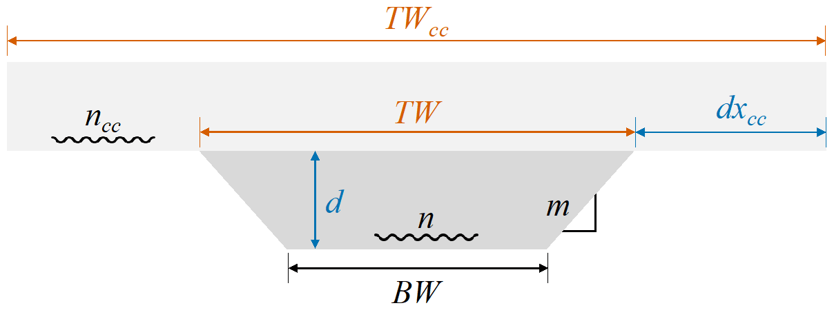
Figure 1Cross-sectional diagram of the trapezoidal channel schematic used in the channel routing module of the NWM. This compound channel representation consists of a main channel (dark gray) and a floodplain (light gray) which becomes inundated in times of overbank flooding in the main channel. Parameters in blue were used to compute the parameters in orange for consistency among inputs for the sensitivity analysis. Parameters in black remained unchanged.
2.3 Sensitivity analysis
A sensitivity analysis was conducted to establish the influence of channel parameters on model streamflow output (Pianosi et al., 2016). To generate combinations of values within the parameter set, a Latin hypercube sampling (LHS) method was used to systematically sample across a hyperdimensional space. LHS is based on the Latin square design, which contains a single sample in each row and column of a hypothetical square with edges representing the ranges of two parameters (McKay et al., 1979). In this method, cumulative density functions (CDFs) for each parameter are divided into equal partitions, and data points within each partition are selected and randomly combined with other selected parameter values. LHS was chosen as it offers an advantage over random sampling techniques by ensuring representativeness of the real variability among the parameters of each randomly selected combination.
Given a lack of strict boundary conditions for the parameter values, inputs were instead varied as a function of their nominal values developed from regional curve relationships with drainage area (for estimating geometry parameters), following Blackburn-Lynch et al. (2017) and the expert opinion scaled by Strahler stream order (for estimating Manning's n parameters). These were compared to the resulting variation in model output expressed as a fraction of the output under the default parameterization. Parameters were modified between a factor of 0.1 and 10 of their nominal values in an effort to encompass the range of possible error in parameter values. Uniform distributions of parameter scalars in the [0.1,10] space were generated and combined using the randomLHS function of the lhs R package (Carnell, 2020) and subsequently multiplied with the relevant default parameters. Here, d and dxcc were calculated from the original data using Eqs. (1)–(2), combined with multipliers, and transformed back to the original parameter space.
We employ the variance-based method of Sobol' (2001) for analysis of the NWM channel routing module parameter sensitivity, following the precedent set by many prior sensitivity analyses of hydrologic models (e.g., Abebe et al., 2010; Baroni and Tarantola, 2014; Cibin et al., 2010; Herman et al., 2013; Massmann and Holzmann, 2012; Nossent et al., 2011; Pappenberger et al., 2008; Reusser et al., 2011; Song et al., 2012; Tang et al., 2007; Wagener et al., 2009; Yang, 2011; Zelelew and Alfredsen, 2013). Specifically, we follow the method of Saltelli (2002), using the sobolSalt function within the sensitivity R module (Iooss et al., 2021) to estimate the first-order (the influence of each parameter alone) and total effect (first order plus all interactive effects) indices, which implements a Monte Carlo estimation of the Sobol' indices at a cost of evaluations, where n is sample size, and p is the number of parameters.
A total of n=3360 unique channel parameter sets (70 groups of 48 members each) for p=6 parameters were tested in each of 12 basins distributed across CONUS over an 8-year period from 1 October 2010 to 30 September 2018 (Fig. 2). Because running the analysis over all of CONUS is computationally prohibitive, these basins were selected to represent variability in NWM calibration basins over CONUS. Calibration basins minimize volume errors, while the 12 basins span a wide range of climate, land cover, and terrain conditions.
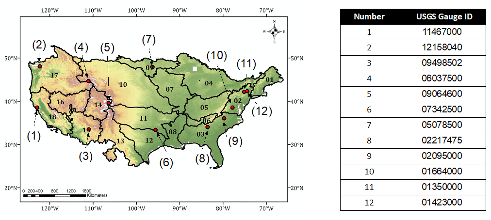
Figure 2Map of study domains, with red points showing locations for 12 representative basins dispersed across CONUS used for the channel routing module sensitivity analysis. These numbers correspond to the USGS gauge IDs listed in the table. Numbers and boundaries on the map correspond to the 18 designations and the extents of Hydrologic Unit Code (HUC)2 regions.
A collection of output metrics describing model fit to observed data, including normalized mean bias (NMB; Yu et al., 2006), Nash–Sutcliffe efficiency (NSE; Nash and Sutcliffe, 1970), and Richards–Baker flashiness index (R–B index; Baker et al., 2004), were used to reduce the model output time series to scalar values more readily comparable to the input parameter set. Equations for these metrics are provided below, as follows:
where M is the model streamflow, O is observed streamflow, i is the time step, and N is the total number of time steps. The optimal value for NMB is 0 %, the optimal value for NSE is 1, and the optimal R–B index is 1, which matches observations. Normalized mean bias provides an unbiased, symmetric measure of tendency to overpredict or underpredict scaled by the output flow values, NSE is a widely used measure of model GOF to the overall observational time series, and R–B index flashiness evaluates how short-term changes in streamflow are affected by the channel routing parameterization. These metrics were selected as they each provide unique insights into model performance and have previously been effectively used for the evaluation of hydrologic models in similar applications (e.g., Avellaneda and Jefferson, 2020; McInerney et al., 2018; Wu et al., 2012; Yeste et al., 2020).
2.4 Channel parameter development
Channel parameters were first estimated at HyG-associated NHD reach segments and then subsequently estimated at all CONUS river reaches through a regression-based regionalization approach. The at-a-station hydraulic geometry of a channel (AHG) was calculated by relating the cross-sectional variation in stream discharge with width, depth, and velocity using power law relationships (Leopold and Maddock, 1953), as follows:
where w is width, d is depth, v is velocity, Q is discharge (equal to the product of w, d, and v), a, c, and k are fitted coefficients which must multiply to 1, and b, f, and m are fitted exponents which must sum to 1. Using the field measurements of Q available in HyG, we first estimated the fitted coefficients (a, c, and k) and exponents (b, f, and m) at each HyG location. For a given flow percentile, variables w, d, and v were then calculated using the fitted values in Eqs. (6)–(8).
Manning's n was estimated using w, d, v, and longitudinal slope (S) via Eqs. (9) and (10), as follows:
where R is the hydraulic radius. Equation (10) is a version of the Manning's equation. Generally, longitudinal water surface slope is not measured at USGS and state stream gauging locations. Instead, values for slope were obtained from the NHDPlus dataset attribute ElevSlope, a longitudinally smoothed slope product produced from topographic data (USGS, 2001).
For estimating the channel geometry parameters of BW and m used in the NWM routing model, a half-channel conceptualization was used. For a given gauge, field measurements of and d together allow for calculation of the channel side slope. This was fit through a linear regression, as follows:
and the point where d=0 along this fitted line is taken to be (BW). The slope of this fit is the channel side slope (m). TW was estimated as the width of the channel at a high percentile flow (e.g., 99th or 99.9th), which was analyzed through the model validation described in Sect. 2.6.
2.5 Regionalization analysis
We conducted an analysis of the regionalization method using the Manning's n parameter as a representative for the full suite of channel parameters described in Fig. 1, given the importance of roughness defined in prior studies. Manning's n was regionalized to unobserved channels in the stream network using a regression-based method. We fit linear regressions between log-transformed Manning's n and S at a flow percentile, i, as follows:
where m is the slope of the regression line, and b is the intercept.
Training of the regionalization regression equations for Manning's n was performed at three spatial scales, i.e., HUC4, HUC2, and the full CONUS-wide domain. For each scale, only the observed data available within each spatial unit of that scale were used to estimate at reaches within that unit. The purpose of this multiscale analysis was to attribute error in estimated Manning's n to variation in scale. In other words, maximization of available observations to fit the Eq. (9) regression and minimization of regression error are competing objectives, such that the scale which results in the least error may vary by location. Similarly, because Manning's n may vary based on the flow percentile used to estimate them (e.g., Eq. 8), the regionalization was conducted using a range of flow percentiles at HyG locations, including the 50th, 75th, 90th, 95th, and 99th percentile flow values. The variation across three spatial scales and five flow percentiles results in a 3×5 matrix of estimated Manning's n values at HyG locations.
To facilitate a standardized method for evaluating the regionalization, a k-fold cross-validation (CV) was performed using a value of k=10 folds. In this approach, training data were randomly divided into 10 equal-sized groups, and we systematically withheld one group at a time while training the model with the remaining nine. We then predicted Manning's n for the withheld group and compared regression-predicted values with the HyG-derived estimates.
2.6 CONUS-wide evaluation experiments
To understand the regional- and national-scale implications of new channel parameters, the NWM routing module was run across the entirety of the 2.7×10⁶ CONUS reaches, over a period of 8 years from 1 October 2010 to 30 September 2018. As only the routing module was run (i.e., not the LSM), total channel inflow volumes remained fixed across experiments, such that any variation may be attributable to routing parameterization. Here, nine channel parameter set configurations were used, in addition to the v2.1 default configuration, for a total of 10 experimental trials. These configurations included parameter sets with Manning's n regionalized at HUC4, HUC2, and full CONUS-wide domain spatial scales using 95th percentile flows. Channel geometry sets included default parameter values along with HUC4-scale regionalized estimates, with TW calculated using either the 99th (TW99) or 99.9th (TW99.9) percentile flows. This creates a 3×3 matrix of Manning's n and geometry combinations in addition to the default parameterization (Fig. 3).
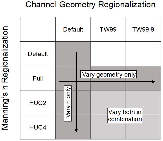
Figure 3Summary of Manning's n and channel geometry configurations used for the routing module simulations conducted across CONUS. Dark gray boxes indicate configurations where only Manning's n or channel geometry were updated from the default parameterization, and light gray boxes indicate configurations where both were modified.
The experimental trials were evaluated with the objective of identifying whether errors affecting the GOF metrics performance were reduced relative to the default configuration. This evaluative approach was used because the routing module only controls the flow routing through the system rather than total flow volume. We compared the hourly streamflow output of each trial at observed reaches CONUS-wide, using available gauge observations, and also conducted a closer examination of simulated flows for a selection of individual gauges from the 12 representative basins (Fig. 2). For the CONUS-wide analysis, GOF metrics such as percent bias (Eq. 3), NSE (Eq. 4), and R2 were calculated at each stream gauge. The difference between median experimental trial output metrics and default output metrics was used to quantify where and how updates to channel parameterization resulted in the greatest differences. The variance among experimental trial output metrics was also examined to further characterize agreement among trials.
3.1 Sensitivity analysis
Across all calculated metrics and domains, Manning's n was shown to hold the highest first-order and total effect sensitivity indices, indicating a higher sensitivity of the model output to Manning's n (Fig. 4). The difference between Manning's n and other channel parameter sensitivities varied considerably across these dimensions, however. Normalized bias in comparison to gauge observations showed increased sensitivity for other parameters relative to Manning's n across all basins, particularly BW and ncc, for total effect sensitivity.
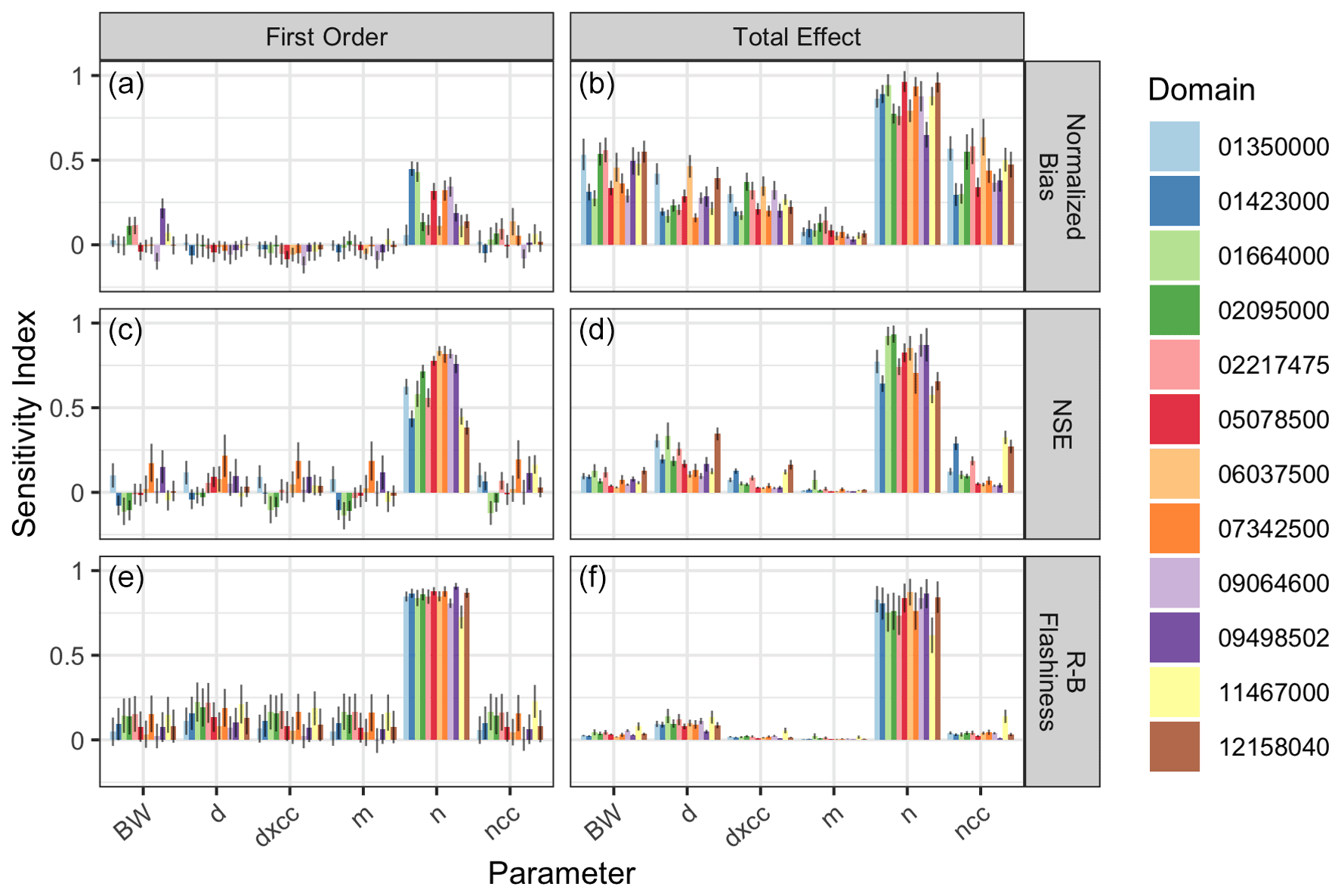
Figure 4Sensitivity analysis results for the NWM channel routing module in 12 representative basins (Fig. 1). Estimated first-order indices are listed in panels (a), (c), and (e), and total effect indices are in panels (b), (d), and (f). Indices closer to 1 indicate higher sensitivity, and values less than 0 occur due to numerical instabilities within insensitive variables. Rows represent each of three metrics used to reduce the flow time series to scalar values. Bar plot colors correspond to the domains for which the indices to apply.
3.2 Channel geometry regionalization
The regression fit between log (S) and log (ni) varied by location and scale (Fig. 5). The CONUS-wide log-transformed regression fit with 5777 observation points yielded an R2=0.29. At the HUC2 regionalization level, R2 varied from 0.12 in the Texas–Gulf region (12) to 0.66 in the Great Basin region (16), with an overall median R2=0.37 and median observation count of 290 points in each HUC2. At the HUC4 level, the variance was even greater, with R2 falling between and 0.9 for subregions 0302 and 0704, respectively. Overall, the median R2=0.45 and median observation count was 26 points per spatial unit. At this scale, there is also an apparent east to west gradient of decreasing error, largely due to the presence of low R2 HUC4 basins in the Texas–Gulf (12) and South Atlantic–Gulf (03) regions. Kernel density plots for errors in Manning's n subdivided by regionalization scale and HUC2 region are shown in Fig. A1.
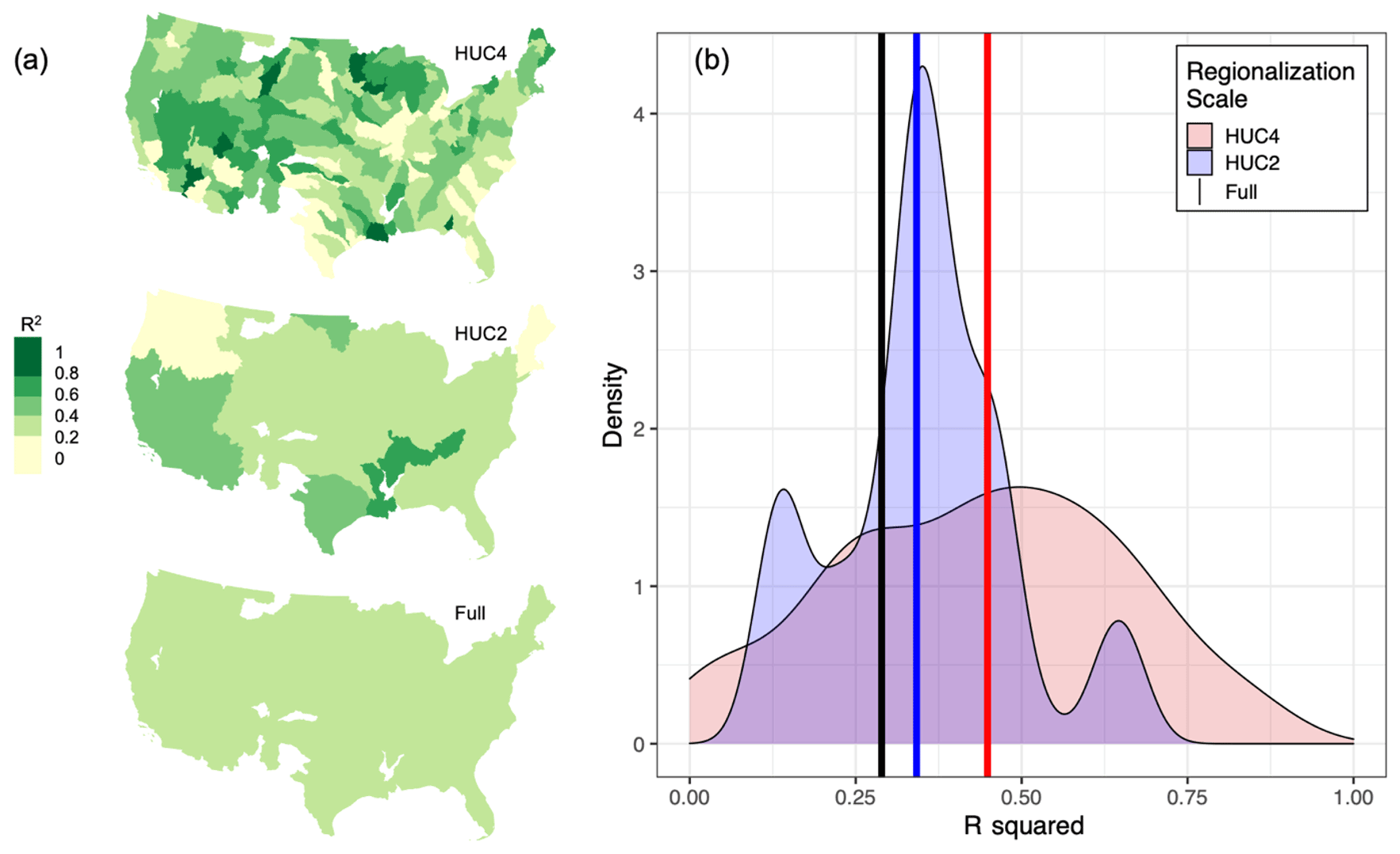
Figure 5Summaries of R2 values resulting from the regression fit of Manning's n as a function of channel longitudinal slope at HUC4, HUC2, and full CONUS domain regionalization scales. Panel (a) shows a spatial breakdown of R2 values at units within each scale, and panel (b) shows kernel density plots for regressions made at the HUC4 and HUC2 scales, with vertical lines denoting the R2 from the full CONUS-wide fit and the median values for the HUC4 and HUC2 scales.
CV results from the 3×5 matrix of regionalization scale and flow percentile combinations are summarized in Fig. 6. General patterns of decreasing error with increasing flow percentile and finer scale were evident, with some exceptions. For example, the regression determined from 90th percentile flow yielded the smallest Manning's n error in the California region (18), whereas the smallest error in the Tennessee region (06) was achieved at the full CONUS-wide regionalization scale. However, channels in mountainous west HUC2 regions (e.g., 13–17) were poorly represented by the regression made at the full CONUS-wide scale, as evident by the relatively strong underestimation of Manning's n.
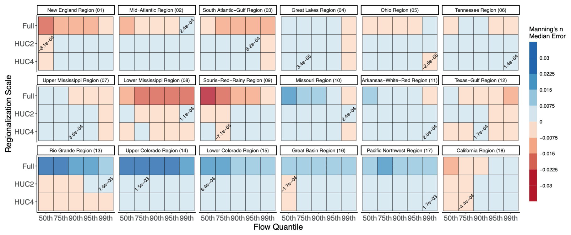
Figure 6A summary of median error in Manning's n resulting from a k-fold CV (k=10) across the matrix of tested regionalization scale and flow percentile combinations. HUC2 regions are shown in each facet, and boxes with text indicate the combination that resulted in the lowest error, which is shown within the box.
Overall, nearly half of the HUC2 regions (8 of 18) showed the 99th percentile as the optimal flow percentile. However, the optimal regression fit was relatively balanced between the HUC2 and HUC4 regionalization scales, with eight regions minimizing the error at HUC2 scale and nine regions minimizing the error at the HUC4 scale. Variability in the error was highest in the lower Mississippi region (08), where the ratio between slope and Manning's n varied greatly among observed locations and there were fewer observations (Fig. A2). In the western regions (e.g., 13–17), a strong positive bias in the estimated Manning's n at the full CONUS-wide regionalization scale was evident.
3.3 CONUS-wide channel parameters
In comparison to the default parameterization, the experimental parameter combinations described in Fig. 3 resulted in substantial differences to both the estimated Manning's n and channel cross-sectional area (Fig. 7), with the HUC4 regionalization and TW99.9 geometry configuration presenting the greatest differences from the default version. The majority of the channels (76 %) are represented in the default NWM version by a Manning's n value of 0.06. The regionalized Manning's n updated these values to a new range between 0.006 and 0.537 (median =0.077), most noticeably in mountainous headwaters regions, where roughness increased by approximately 200 % under the HUC4 regionalization scheme. Similar changes were also apparent under the HUC2 (0.007 to 0.436; median =0.076) and full regionalization schemes (0.012 to 0.436; median =0.072), albeit to a lesser extent. Overall, the variance of Manning's n across CONUS increased with smaller regionalization spatial scales. Similar magnitudes of change were evident in the channel cross-sectional area. Compared to the default geometry parameterization cross-sectional area (0.018 to 1990 m2; median =2.03 m2), the TW99 configuration ( to 8610 m2; median =0.927 m2) and TW99.9 configuration ( to 7150 m2; median =2.08 m2) both resulted in wider ranges, though the median area for TW99 was reduced by an order of magnitude, and this reduction was largely observable at reaches located across the west. However, in the lower Mississippi region (08), the cross-sectional area of the channel increased by approximately 200 % under the new regionalization schemes.

Figure 7Spatial maps illustrating default parameterizations, updated parameterizations, and their percent differences across CONUS for Manning's n and the channel-geometry-derived cross-sectional area at a random subsample of 1 % of the 2.7×10⁶ NHD-derived reaches across CONUS. Panels (a) and (b) describe the default and HUC4-regionalized Manning's n parameter, panels (d) and (e) describe the default and TW99.9 configuration cross-sectional area, and panels (c) and (f) show the percent differences between default and updated parameterizations for Manning's n and cross-sectional area, respectively.
Across the 6841 USGS gauge locations with continuous information across the experimental period, the median percent difference between default Manning's n and the HUC4-regionalized Manning's n was approximately −9 %, with a standard deviation σ=61 % (HUC2 – median % and σ=52 %; full – median % and σ=49 %). For the channel cross-sectional area using 99th percentile flow to estimate top width (TW99), this difference was −32 %, with a standard deviation σ=47 % (TW99.9 – median =17 % and σ=88 %). Generally, the median channel size was reduced in the TW99 configuration and increased in the TW99.9 configuration (Fig. 8).
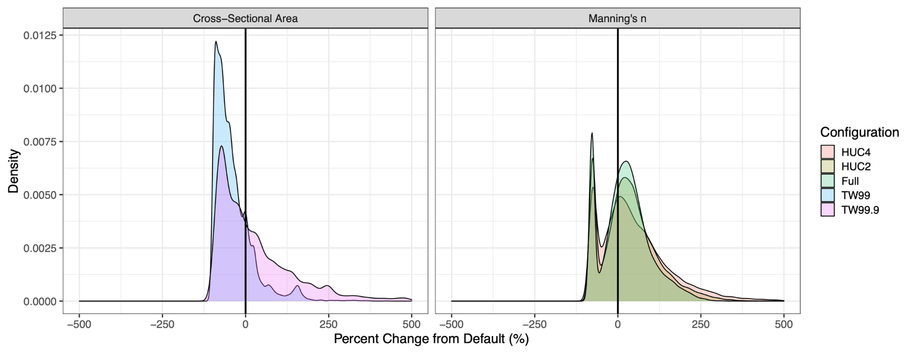
Figure 8Density plots of percent changes in cross-sectional area and Manning's n from default parameter values across CONUS under experimental trial configurations.
3.4 CONUS-wide evaluation experiments
Among the experimental trials, variance was generally low (approx. ) in the bulk GOF metrics calculated from the model output at gauge locations, indicating little difference in model output among the updated channel parameter sets resulting from modifying routing module parameterization alone. Yet, differences between median experimental trial output metrics and the default output metrics yielded some measurable differences, particularly for the agreement index () and R2 () metrics. Effects on performance were negligible across most gauges, with the median value for each metric approximately 0 in all cases (Fig. 9). Spatial maps for other metrics are provided in Fig. A3.
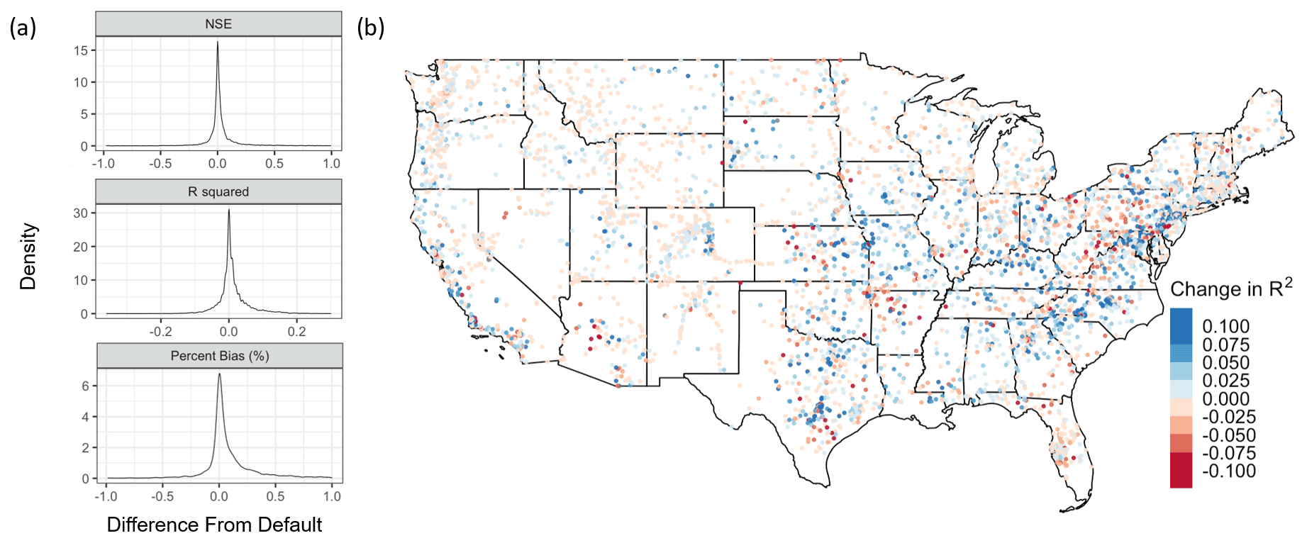
Figure 9Summary metrics at 4655 USGS gauge locations for the HUC4 regression scale and the TW99.9 combination experimental trial calculated across CONUS-wide gauge locations. Panel (a) shows faceted density plots for each difference in that metric from the default parameterization, and panel (b) shows the Pearson correlation among the metrics.
Overall, mean R2 across gauges increased from the default parameterization (mean R2=0.479) for all experimental trials (from a mean R2=0.489 for the full TW99 configuration to a mean R2=0.494 for the HUC4 TW99.9 configuration). The HUC4 TW99.9 configuration also resulted in the largest overall influence on the model output overall (i.e., regardless of whether performance improved or worsened), which is consistent with the degree of perturbation made to the channel parameters relative to other configurations.
3.5 Analysis at selected gauges
Of the 12 representative basins (Fig. 2), two gauges at outlets were selected for further examination based on the relatively high degree and opposing directions of change made to the parameterization of Manning's n and channel geometry relative to the default parameterization and differences in basin physiography and climate. The first is USGS gauge 09064600 at Eagle River near Minturn, CO. This gauge is located in the mountainous headwaters region of the Colorado River basin (elevation 2467 m) and monitors flow over a drainage area of 482 km2. From a default value of 0.055, Manning's n was increased for this gauged reach to 0.078, 0.073, and 0.097 for HUC4, HUC2, and full regionalization scales, respectively. The cross-sectional area was reduced from a default of 19.9–4.9 and 6.4 m2 for TW99 and TW99.9 configurations, respectively. The second is USGS gauge 01664000 at Rappahannock River near Remington, VA. This gauge is located at a lower elevation (92 m) and monitors flow over a greater drainage area of 1603 km2. In contrast to the Colorado gauge, the default value of 0.050 for Manning's n was decreased for this channel to 0.017, 0.015, and 0.015 for HUC4, HUC2, and full regionalization scales, respectively. The cross-sectional area was altered from a default of 37.5–35.4 and 65.7 m2 for TW99 and TW99.9 configurations, respectively.
Noticeable differences in the behavior across the experimental scenario results exist between the two selected gauges (Fig. 10). While NSE, R2, and RMSE were relatively consistent across experimental trials for gauge 09064600, there is a noticeable trend of decreasing performance from the default parameterization run and updated Manning's n runs when the channel geometry is updated. The highest differences across experiments were those where channel geometry alone was perturbed. NSE was 0.50 for the default parameterization and 0.51, 0.44, and 0.41 for the default geometry with updated Manning's n only, the TW99 channel geometry parameterization, and the TW99.9 channel geometry parameterization, respectively. By contrast, experimental performance among trials where only Manning's n was perturbed were relatively consistent and higher than the default parameterization for both gauges. For gauge 09064600, R2 increased from the default parameterization (R2=0.77) for all runs, with the highest increase seen for the HUC4 TW99.9 run (R2=0.81).
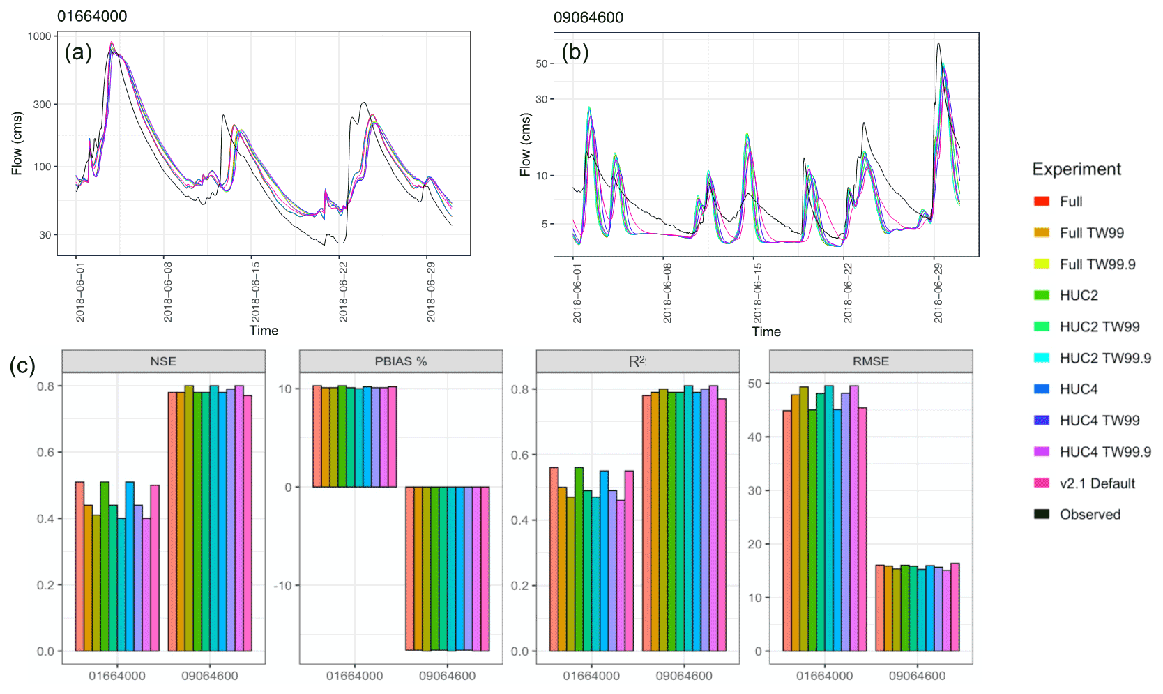
Figure 10A summary of experimental results at two gauge locations. Panels (a) and (b) describe hydrographs for USGS gauge 09064600 and USGS gauge 01664000, respectively, for 1 example month in June 2018, and panel (c) shows metric results computed across the entire hydrograph at each gauge location for NSE, percent bias, R2, and RMSE.
Results from the sensitivity analysis showed that channel roughness (Manning's n) holds a stronger influence on modeled streamflow than channel dimensions in the routing module. This finding is supported by prior literature suggesting that Manning's n is a significant determinant of flood wave celerity (Anderson et al., 2006) and serves to attenuate and delay the arrival of peak discharge at the catchment outlet (Wolff and Burges, 1994; Woltemade and Potter, 1994). In the NWM, attenuation is modeled through the Muskingum–Cunge method of flood routing (Cunge, 1969), which uses a diffusion wave representation subject to attenuation as it propagates through a channel network. The relative sensitivity of model output variance to Manning's n suggests that the most efficient optimization strategy for improving representation in the channel routing module is one that is focused on updating Manning's n. However, the overall results from the experimental simulations showed that runs where channel geometry was varied in isolation generally yielded a higher variance in model output than runs where Manning's n was varied in isolation. Such results show that combinatory effects among the channel geometry parameters may result in a stronger influence over the model hydrograph in comparison with varying the Manning's n parameter alone. The case for updating all geometry parameters is strengthened by the fact that the HUC4 TW99.9 configuration, containing the most extreme perturbations of all parameters, was found to increase R2 by the largest degree.
Though the results were largely conclusive, several aspects of the sensitivity analysis may be modified in potential future studies. For example, the selected boundary conditions ranged from 0.1 to 10 times the nominal parameter values, which may not be reflective of the true uncertainty in these parameter values. The possibility also exists that parameter sensitivity is flow dependent, which may be most obvious in the case of the parameters TWcc and ncc, as flow depth is often too low to reach the floodplain. Consideration for observational error in channel parameters and/or running the model in data assimilation mode may address this possibility and provide added value in future analyses.
The regionalization of channel parameters was performed using a HUC-based approach, where discrete regions were used to define the regression curves used to estimate channel parameters within those regions. The principal finding in comparing regionalization scales was that a smaller scale typically results in the lowest error (e.g., Fig. 6), and the magnitude of this difference is likely dependent on the inherent spatial variability in the region in which the regressions were developed. For example, the relatively poor performance of the full regression in the topographically variable, mountainous HUC2 regions demonstrate the non-representativeness of regressions developed using all measurements across CONUS for these unique and topographically complex areas. Furthermore, the strong performance of the HUC4 regionalization scale relative to HUC2 in the Missouri region (10) speaks to the diversity of terrain conditions within this region, as it encapsulates both mountainous terrain in the west and flatter plains in the east. Overall, these findings underscore the importance of taking into account the spatial variability in the Manning's n and longitudinal slope relationship. Additional variables which demonstrate strong relationships with channel properties may also be viable for future regressions. For example, height above nearest drainage (HAND) has been used to derive hydraulic properties for reaches along a river network and generate synthetic rating curves relating flow to water level (Zheng et al., 2018).
The HUC-based discretization method, coupled with differences in observational data uncertainty and availability, naturally creates discontinuities at HUC boundaries in the regression parameters. Alternative regionalization approaches may help to alleviate or even remove the errors arising from these discontinuities; for example, a downstream hydraulic geometry (DHG)-based regionalization approach that takes into account observational data from nested gauges within the network to generate channel parameters along a flow path is one possibility that has seen previous success (Allen et al., 2018; Neal et al., 2015).
The estimation of regional regression curves for Manning's n was performed across multiple flow percentiles, as it was found that the regression parameters varied depending on flow. Here, the objective was to identify a singular optimal flow percentile that resulted in the lowest error in the regionalized Manning's n parameter. However, in nature, the celerity and attenuation of a flood wave varies nonlinearly with flow, despite standard engineering practice typically involving the use of the Muskingum–Cunge flood wave representation due to ease of implementation (i.e., a constant Manning's n), which is the case for the NWM. Future improvements to the NWM may consider allowing Manning's n to vary with flow, as this may achieve a better representation of channel hydraulics.
With only a modest sensitivity of model output to channels parameters, results from both the sensitivity analysis and simulations demonstrate the limited influence of the channel routing module to improve GOF metrics within the overall NWM framework. In most cases, low variability in GOF metrics among trials is evident; though in some instances, such as at USGS gauge 09064600, there is some identifiable improvement from the default parameterization. Yet, even here, model hydrographs were unable to match observations. This is expected, as total volume is unaffected by the routing module, and thus the mass is conserved regardless of channel parameterization. However, in the course of model improvement, an appropriate philosophy is to do no harm, which largely characterizes the outcome of these experiments.
Parameters within the Noah-MP LSM not included in the sensitivity analysis or regionalization are likely the source of a large percentage of error, with meteorology and physics representations representing other potential sources. A previous sensitivity analysis conducted on the Noah-MP model indicated high sensitivities for output states and fluxes such as sensible and latent heat, soil moisture, and net ecosystem exchange derived from soil and vegetation parameters (Arsenault et al., 2018). Another showed sensitivity for latent heat and total runoff attributable to two-thirds of applicable standard parameters and the highest sensitivity derived from a hard-coded parameter value in the model used in the formulation of soil surface resistance for direct evaporation (Cuntz et al., 2016). Given these results, future efforts focused on the joint calibration of the Noah-MP LSM and channel routing module may result in noticeable GOF metrics improvements.
This analysis explored the effects of modifying channel routing parameters in the National Water Model streamflow simulations using a regionalized hydraulic geometry and Manning's n dataset. Based on a sensitivity analysis conducted on a selection of channel parameters in the routing module, it can be concluded that the Manning's n roughness coefficient holds an outsized effect on modeled flow relative to parameters which describe the channel geometry. Yet, results from experimental simulations of nine alternative parameter configurations showed that the interactive effects among geometry parameters in some geographic regions may be greater than the Manning's n parameter alone.
New estimates of NWM channel parameters following a regression-based regionalization approach generally results in a larger distribution of channel characteristics over the NWM v2.1 default parameterization. Overall, variance in both Manning's n and cross-sectional area among channels CONUS-wide increased from the default parameterization, which also accompanied a modest increase to median R2 across gauge locations as well, from 0.479 to 0.494 for the HUC4 TW99.9 configuration.
For Manning's n, approximately 76 % of channels in the default parameterization are currently represented by the same nominal value of 0.06 (18 % with a value of 0.055 and lesser percentages at further intervals of 0.005) and are not based on observations but rather expert opinion, which is scaled by the Strahler stream order. A new HyG-based Manning's n representation provides an observational foundation for Manning's n, which consequently increases roughness across mountainous headwaters regions and decreases roughness in lowlands and coastal areas to a new range between 0.006 and 0.537 (median 0.077), qualitatively changing the distribution.
Channel geometry updates resulted in a longitudinal gradient in the percent change in the cross-sectional area. In the east, and particularly in the lower Mississippi region, the cross-sectional area increased, while a decrease in area is visible throughout smaller streams in the more arid west.
The influence of the routing module over modeled streamflow GOF metric performance is limited compared to other components of the NWM framework, such as the land surface model and meteorological input data. Future approaches towards the calibration of the NWM may yield the largest benefits through a more holistic approach to calibrating the overall framework, i.e., a comprehensive evaluation and calibration of all model components. Towards this objective, our characterization of the overall effects of strengthening channel routing module parameter representativeness may serve as an important foundation for the further improvement of the NWM and hydrologic modeling in CONUS. In turn, the NWM becomes better positioned to meet the stated goal of providing quality, actionable guidance for the mitigation of flood-related damages.
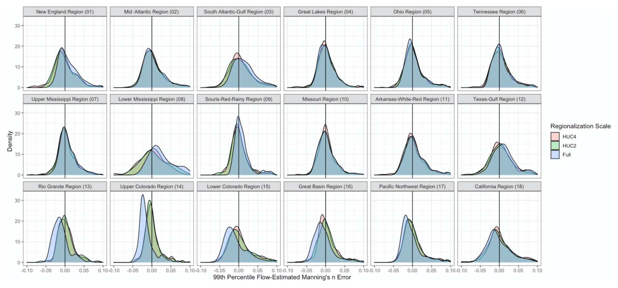
Figure A1Kernel density plots showing the range of Manning's n error resulting from each regression-based regionalization scale at gauge locations, including full CONUS-wide (blue), HUC2 (green), and HUC4 (red). Facets indicate the HUC2 region in which the gauges are located.
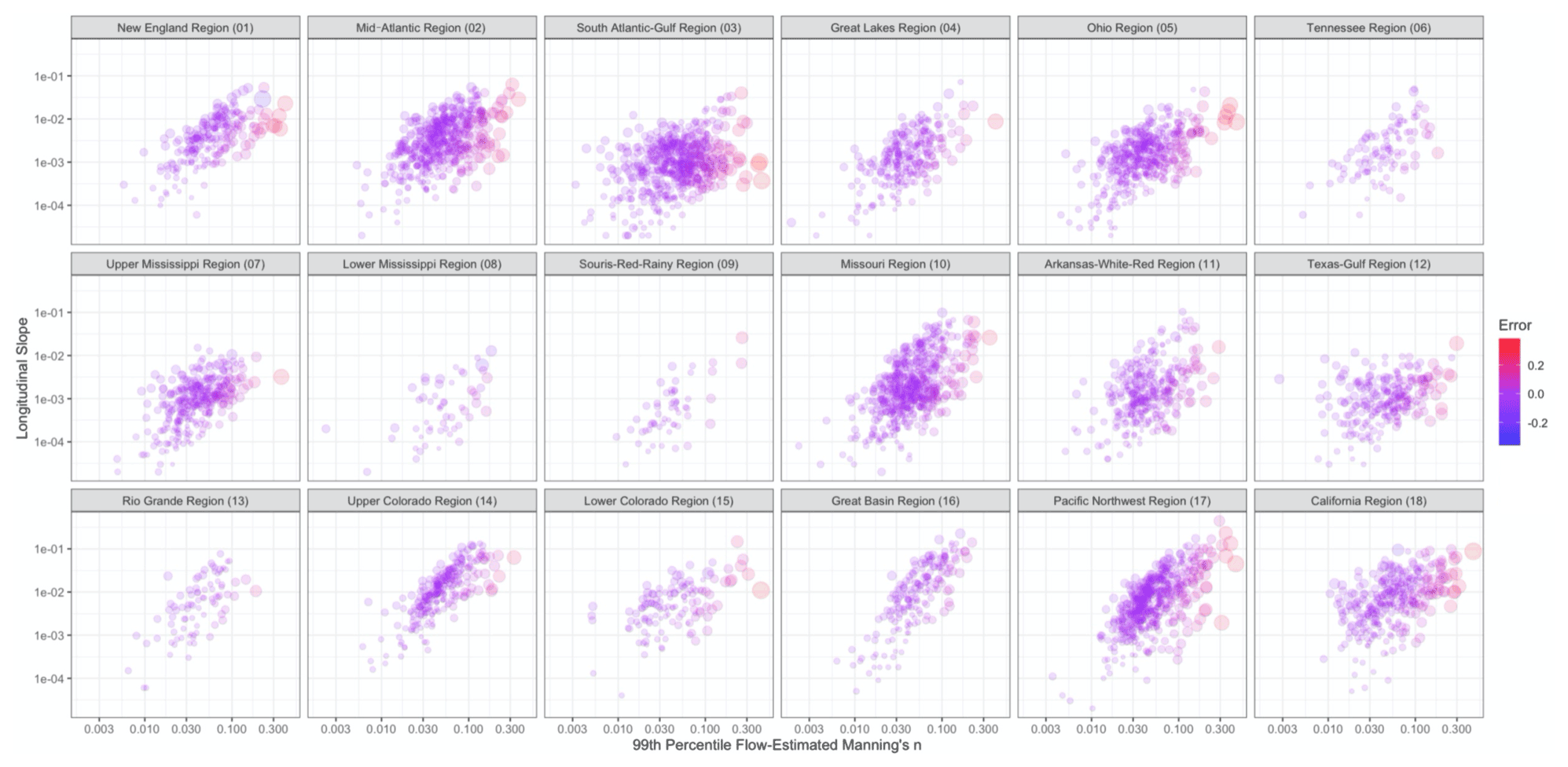
Figure A2Scatterplots of log-transformed longitudinal slope (S) and Manning's n (n) estimated at 99th percentile flows for HyG locations in each HUC2 region are shown. The size of the points indicate the magnitude of error in the regression, and color indicates an underestimate (blue) or overestimate (red).

Figure A3Spatial maps describing change in the agreement index, NSE, bias, and percent bias from default parameterization performance at USGS gauge locations across CONUS.
The underlying code and data are available upon request from the corresponding author.
AH conducted the evaluation and wrote the manuscript. BL provided advice and edited the manuscript. JM and LR provided model output data and served as points of contact for model operations. JK edited the manuscript. TM provided the dataset used in the evaluation and gave advice.
The contact author has declared that none of the authors has any competing interests.
Publisher’s note: Copernicus Publications remains neutral with regard to jurisdictional claims in published maps and institutional affiliations.
This research has been supported by the National Oceanic and Atmospheric Administration (grant no. NA18OAR4590391).
This paper was edited by Pieter van der Zaag and reviewed by two anonymous referees.
Abdulla, F. A. and Lettenmaier, D. P.: Development of regional parameter estimation equations for a macroscale hydrologic model, J. Hydrol., 197, 230–257, https://doi.org/10.1016/S0022-1694(96)03262-3, 1997.
Abebe, N. A., Ogden, F. L., and Pradhan, N. R.: Sensitivity and uncertainty analysis of the conceptual HBV rainfall–runoff model: Implications for parameter estimation, J. Hydrol., 389, 301–310, https://doi.org/10.1016/j.jhydrol.2010.06.007, 2010.
Allen, G. H., Pavelsky, T. M., Barefoot, E. A., Lamb, M. P., Butman, D., Tashie, A., and Gleason, C. J.: Similarity of stream width distributions across headwater systems, Nat, Commun,, 9, 610, https://doi.org/10.1038/s41467-018-02991-w, 2018.
Anderson, B. G., Rutherfurd, I. D., and Western, A. W.: An analysis of the influence of riparian vegetation on the propagation of flood waves, Environ. Modell. Softw., 21, 1290–1296, https://doi.org/10.1016/j.envsoft.2005.04.027, 2006.
Arsenault, K. R., Nearing, G. S., Wang, S., Yatheendradas, S., and Peters-Lidard, C. D.: Parameter Sensitivity of the Noah-MP Land Surface Model with Dynamic Vegetation, J. Hydrometeorol., 19, 815–830, https://doi.org/10.1175/jhm-d-17-0205.1, 2018.
Avellaneda, P. M. and Jefferson, A. J.: Sensitivity of Streamflow Metrics to Infiltration-Based Stormwater Management Networks, Water Resour. Res., 56, e2019WR026555, https://doi.org/10.1029/2019WR026555, 2020.
Ayzel, G. V., Gusev, E. M., and Nasonova, O. N.: River runoff evaluation for ungauged watersheds by SWAP model. 2. Application of methods of physiographic similarity and spatial geostatistics, Water Resour., 44, 547–558, https://doi.org/10.1134/S0097807817040029, 2017.
Baker, D. B., Richards, R. P., Loftus, T. T., and Kramer, J. W.: A New Flashiness Index: Characteristics and Applications to Midwestern Rivers and Streams, J. Am. Water Resour. As., 40, 503–522, https://doi.org/10.1111/j.1752-1688.2004.tb01046.x, 2004.
Baroni, G. and Tarantola, S.: A General Probabilistic Framework for uncertainty and global sensitivity analysis of deterministic models: A hydrological case study, Environ. Modell. Softw., 51, 26–34, https://doi.org/10.1016/j.envsoft.2013.09.022, 2014.
Biancamaria, S., Lettenmaier, D. P., and Pavelsky, T. M.: The SWOT Mission and Its Capabilities for Land Hydrology, in: Remote Sensing and Water Resources, edited by: Cazenave, A., Champollion, N., Benveniste, J., and Chen, J., Springer International Publishing, Cham, 117–147, https://doi.org/10.1007/978-3-319-32449-4_6, 2016.
Bieger, K., Rathjens, H., Allen, P. M., and Arnold, J. G.: Development and Evaluation of Bankfull Hydraulic Geometry Relationships for the Physiographic Regions of the United States, J. Am. Water Resour. As., 51, 842–858, https://doi.org/10.1111/jawr.12282, 2015.
Blackburn-Lynch, W., Agouridis, C. T., and Barton, C. D.: Development of Regional Curves for Hydrologic Landscape Regions (HLR) in the Contiguous United States, J. Am. Water Resour. As., 53, 903–928, https://doi.org/10.1111/1752-1688.12540, 2017.
Burnash, R. J. C., Ferral, R. L., and McGuire, R. A.: A Generalized Streamflow Simulation System: Conceptual Modeling for Digital Computers, U.S. Department of Commerce, National Weather Service, and State of California, Department of Water Resources, 220 pp., 1973.
Canova, M., Fulton, J., and Bjerklie, D.: USGS HYDRoacoustic dataset in support of the Surface Water Oceanographic Topography satellite mission (HYDRoSWOT), U.S. Geological Survey [data set], https://doi.org/10.5066/F7D798H6, 2016.
Carnell, R.: lhs: Latin Hypercube Samples, https://cran.r-project.org/web/packages/lhs/index.html (last access: 26 September 2022), 2020.
Cibin, R., Sudheer, K. P., and Chaubey, I.: Sensitivity and identifiability of stream flow generation parameters of the SWAT model, Hydrol. Process., 24, 1133–1148, https://doi.org/10.1002/hyp.7568, 2010.
Cunge, J. A.: On The Subject Of A Flood Propagation Computation Method (Musklngum Method), J. Hydraul. Res., 7, 205–230, https://doi.org/10.1080/00221686909500264, 1969.
Cuntz, M., Mai, J., Samaniego, L., Clark, M., Wulfmeyer, V., Branch, O., Attinger, S., and Thober, S.: The impact of standard and hard-coded parameters on the hydrologic fluxes in the Noah-MP land surface model, J. Geophys. Res.-Atmos., 121, 10676–10700, https://doi.org/10.1002/2016JD025097, 2016.
Dunne, T. and Leopold, L. B.: Water in Environmental Planning, Macmillan, 852 pp., ISBN-13: 978-0716700791, 1978.
Fares, A., Awal, R., Michaud, J., Chu, P.-S., Fares, S., Kodama, K., and Rosener, M.: Rainfall-Runoff Modeling in a Flashy Tropical Watershed Using the Distributed HL-RDHM Model, J. Hydrol., 519, 3436–3447, https://doi.org/10.1016/j.jhydrol.2014.09.042, 2014.
Gall, M., Borden, K. A., Emrich, C. T., and Cutter, S. L.: The Unsustainable Trend of Natural Hazard Losses in the United States, Sustainability, 3, 2157–2181, https://doi.org/10.3390/su3112157, 2011.
Gitau, M. and Chaubey, I.: Regionalization of SWAT Model Parameters for Use in Ungauged Watersheds, Water, 2, 849–871, https://doi.org/10.3390/w2040849, 2010.
Gochis, D. J., Barlage, M., Cabell, R., Casali, M., Dugger, A., FitzGerald, K., McAllister, M., McCreight, J., RafieeiNasab, A., Read, L., Sampson, K., Yates, D., and Zhang, Y.: The WRF-Hydro® modeling system technical description, Version 5.1.1, NCAR Technical Note, 107 pp., https://ral.ucar.edu/sites/default/files/public/WRFHydroV511TechnicalDescription.pdf (26 September 2022), 2020.
He, L. and Wilkerson, G. V.: Improved Bankfull Channel Geometry Prediction Using Two-Year Return-Period Discharge1, J. Am. Water Resour. As., 47, 1298–1316, https://doi.org/10.1111/j.1752-1688.2011.00567.x, 2011.
Herman, J. D., Kollat, J. B., Reed, P. M., and Wagener, T.: Technical Note: Method of Morris effectively reduces the computational demands of global sensitivity analysis for distributed watershed models, Hydrol. Earth Syst. Sci., 17, 2893–2903, https://doi.org/10.5194/hess-17-2893-2013, 2013.
Heuvelmans, G., Muys, B., and Feyen, J.: Regionalisation of the parameters of a hydrological model: Comparison of linear regression models with artificial neural nets, J. Hydrol., 319, 245–265, https://doi.org/10.1016/j.jhydrol.2005.07.030, 2006.
Iooss, B., Veiga, S. D., Pujol, A. J. and G., Broto, with contributions from B., Boumhaout, K., Delage, T., Amri, R. E., Fruth, J., Gilquin, L., Guillaume, J., Idrissi, M. I., Gratiet, L. L., Lemaitre, P., Marrel, A., Meynaoui, A., Nelson, B. L., Monari, F., Oomen, R., Rakovec, O., Ramos, B., Roustant, O., Song, E., Staum, J., Sueur, R., Touati, T., and Weber, F.: sensitivity: Global Sensitivity Analysis of Model Outputs, https://cran.r-project.org/web/packages/sensitivity/ (26 September 2022), 2021.
Kay, A. L., Jones, D. A., Crooks, S. M., Calver, A., and Reynard, N. S.: A comparison of three approaches to spatial generalization of rainfall–runoff models, Hydrol. Process., 20, 3953–3973, https://doi.org/10.1002/hyp.6550, 2006.
Koren, V., Reed, S., Smith, M., Zhang, Z., and Seo, D.-J.: Hydrology laboratory research modeling system (HL-RMS) of the US national weather service, J. Hydrol., 291, 297–318, https://doi.org/10.1016/j.jhydrol.2003.12.039, 2004.
Leopold, L. B. and Maddock Jr., T.: The hydraulic geometry of stream channels and some physiographic implications, The hydraulic geometry of stream channels and some physiographic implications, U.S. Government Printing Office, Washington, D.C., https://doi.org/10.3133/pp252, 1953.
Li, M., Shao, Q., Zhang, L., and Chiew, F. H. S.: A new regionalization approach and its application to predict flow duration curve in ungauged basins, J. Hydrol., 389, 137–145, https://doi.org/10.1016/j.jhydrol.2010.05.039, 2010.
Livneh, B., Rosenberg, E. A., Lin, C., Nijssen, B., Mishra, V., Andreadis, K. M., Maurer, E. P., and Lettenmaier, D. P.: A Long-Term Hydrologically Based Dataset of Land Surface Fluxes and States for the Conterminous United States: Update and Extensions, J. Climate, 26, 9384–9392, https://doi.org/10.1175/JCLI-D-12-00508.1, 2013.
Massmann, C. and Holzmann, H.: Analysis of the behavior of a rainfall–runoff model using three global sensitivity analysis methods evaluated at different temporal scales, J. Hydrol., 475, 97–110, https://doi.org/10.1016/j.jhydrol.2012.09.026, 2012.
McInerney, D., Thyer, M., Kavetski, D., Githui, F., Thayalakumaran, T., Liu, M., and Kuczera, G.: The Importance of Spatiotemporal Variability in Irrigation Inputs for Hydrological Modeling of Irrigated Catchments, Water Resour. Res., 54, 6792–6821, https://doi.org/10.1029/2017WR022049, 2018.
McKay, M. D., Beckman, R. J., and Conover, W. J.: A Comparison of Three Methods for Selecting Values of Input Variables in the Analysis of Output from a Computer Code, Technometrics, 21, 239–245, https://doi.org/10.2307/1268522, 1979.
Nash, J. E. and Sutcliffe, J. V.: River flow forecasting through conceptual models part I – A discussion of principles, J. Hydrol., 10, 282–290, https://doi.org/10.1016/0022-1694(70)90255-6, 1970.
Neal, J. C., Odoni, N. A., Trigg, M. A., Freer, J. E., Garcia-Pintado, J., Mason, D. C., Wood, M., and Bates, P. D.: Efficient incorporation of channel cross-section geometry uncertainty into regional and global scale flood inundation models, J. Hydrol., 529, 169–183, https://doi.org/10.1016/j.jhydrol.2015.07.026, 2015.
Niu, G.-Y., Yang, Z.-L., Mitchell, K. E., Chen, F., Ek, M. B., Barlage, M., Kumar, A., Manning, K., Niyogi, D., Rosero, E., Tewari, M., and Xia, Y.: The community Noah land surface model with multiparameterization options (Noah-MP): 1. Model description and evaluation with local-scale measurements, J. Geophys. Res., 116, D12109, https://doi.org/10.1029/2010JD015139, 2011.
Nossent, J., Elsen, P., and Bauwens, W.: Sobol' sensitivity analysis of a complex environmental model, Environ. Modell. Softw., 26, 1515–1525, https://doi.org/10.1016/j.envsoft.2011.08.010, 2011.
Pappenberger, F., Beven, K. J., Ratto, M., and Matgen, P.: Multi-method global sensitivity analysis of flood inundation models, Adv. Water Resour., 31, 1–14, https://doi.org/10.1016/j.advwatres.2007.04.009, 2008.
Pianosi, F., Beven, K., Freer, J., Hall, J. W., Rougier, J., Stephenson, D. B., and Wagener, T.: Sensitivity analysis of environmental models: A systematic review with practical workflow, Environ. Modell. Softw., 79, 214–232, https://doi.org/10.1016/j.envsoft.2016.02.008, 2016.
Reusser, D. E., Buytaert, W., and Zehe, E.: Temporal dynamics of model parameter sensitivity for computationally expensive models with the Fourier amplitude sensitivity test, Water Resour. Res., 47, W07551, https://doi.org/10.1029/2010WR009947, 2011.
Saltelli, A.: Sensitivity Analysis for Importance Assessment, Risk Anal., 22, 579–590, https://doi.org/10.1111/0272-4332.00040, 2002.
Sobol', I. M.: Global sensitivity indices for nonlinear mathematical models and their Monte Carlo estimates, Math. Comput. Simulat., 55, 271–280, https://doi.org/10.1016/S0378-4754(00)00270-6, 2001.
Song, X., Zhan, C., Xia, J., and Kong, F.: An efficient global sensitivity analysis approach for distributed hydrological model, J. Geogr. Sci., 22, 209–222, https://doi.org/10.1007/s11442-012-0922-5, 2012.
Tang, Y., Reed, P., Wagener, T., and van Werkhoven, K.: Comparing sensitivity analysis methods to advance lumped watershed model identification and evaluation, Hydrol. Earth Syst. Sci., 11, 793–817, https://doi.org/10.5194/hess-11-793-2007, 2007.
USGS: National Hydrography Dataset (NHD), U.S. Geological Survey [data set], Reston, VA, https://doi.org/10.3133/70046927, 2001.
Wagener, T., van Werkhoven, K., Reed, P., and Tang, Y.: Multiobjective sensitivity analysis to understand the information content in streamflow observations for distributed watershed modeling, Water Resour. Res., 45, W02501, https://doi.org/10.1029/2008WR007347, 2009.
Wolff, C. G. and Burges, S. J.: An analysis of the influence of river channel properties on flood frequency, J. Hydrol., 153, 317–337, https://doi.org/10.1016/0022-1694(94)90197-X, 1994.
Woltemade, C. J. and Potter, K. W.: A watershed modeling analysis of fluvial geomorphologic influences on flood peak attenuation, Water Resour. Res., 30, 1933–1942, https://doi.org/10.1029/94WR00323, 1994.
Wu, H., Lye, L., and Chen, B.: A design of experiment aided sensitivity analysis and parameterization for hydrological modeling, Can. J. Civil Eng., 39, 460–472, https://doi.org/10.1139/l2012-017, 2012.
Yang, J.: Convergence and uncertainty analyses in Monte-Carlo based sensitivity analysis, Environ. Modell. Softw., 26, 444–457, https://doi.org/10.1016/j.envsoft.2010.10.007, 2011.
Yeste, P., García-Valdecasas Ojeda, M., Gámiz-Fortis, S. R., Castro-Díez, Y., and Esteban-Parra, M. J.: Integrated sensitivity analysis of a macroscale hydrologic model in the north of the Iberian Peninsula, J. Hydrol., 590, 125230, https://doi.org/10.1016/j.jhydrol.2020.125230, 2020.
Yu, S., Eder, B., Dennis, R., Chu, S.-H., and Schwartz, S. E.: New unbiased symmetric metrics for evaluation of air quality models, Atmos. Sci. Lett., 7, 26–34, https://doi.org/10.1002/asl.125, 2006.
Zelelew, M. B. and Alfredsen, K.: Sensitivity-guided evaluation of the HBV hydrological model parameterization, J. Hydroinform., 15, 967–990, https://doi.org/10.2166/hydro.2012.011, 2013.
Zheng, Z., Molotch, N. P., Oroza, C. A., Conklin, M. H., and Bales, R. C.: Spatial snow water equivalent estimation for mountainous areas using wireless-sensor networks and remote-sensing products, Remote Sens. Environ., 215, 44–56, https://doi.org/10.1016/j.rse.2018.05.029, 2018.