Machine-learning-based downscaling of modelled climate change impacts on groundwater table depth

There is an urgent demand for assessments of climate change impacts on the hydrological cycle at high spatial resolutions. In particular, the impacts on shallow groundwater levels, which can lead to both flooding and drought, have major implications for agriculture, adaptation, and urban planning. Predicting such hydrological impacts is typically performed using physically based hydrological models (HMs). However, such models are computationally expensive, especially at high spatial resolutions.

This study is based on the Danish national groundwater model, set up as a distributed, integrated surface–subsurface model at a 500 m horizontal resolution. Recently, a version at a higher resolution of 100 m was created, amongst others, to better represent the uppermost groundwater table and to meet end-user demands for water management and climate adaptation. However, the increase in resolution of the hydrological model also increases computational bottleneck. To evaluate climate change impacts, a large ensemble of climate models was run with the 500 m hydrological model, while performing the same ensemble run with the 100 m resolution nationwide model was deemed infeasible. The desired outputs at the 100 m resolution were produced by developing a novel, hybrid downscaling method based on machine learning (ML).

Hydrological models for five subcatchments, covering around 9 % of Denmark and selected to represent a range of hydrogeological settings, were run at 100 m resolutions with forcings from a reduced ensemble of climate models. Random forest (RF) algorithms were established using the simulated climate change impacts (future – present) on water table depth at 100 m resolution from those submodels as training data.

The trained downscaling algorithms were then applied to create nationwide maps of climate-change-induced impacts on the shallow groundwater table at 100 m resolutions. These downscaled maps were successfully validated against results from a validation submodel at a 100 m resolution excluded from training the algorithms, and compared to the impact signals from the 500 m HM across Denmark.

The suggested downscaling algorithm also opens for the spatial downscaling of other model outputs. It has the potential for further applications where, for example, computational limitations inhibit running distributed HMs at fine resolutions.

1 Introduction

Groundwater accounts for a substantial part of the active hydrological cycle, and exhibits a wide range of interactions with ecosystems, food and energy security, as well as climate and flood regulation (Gleeson et al., 2016). Interactions with the land surface and other components of the hydrological cycle are particularly pronounced where the uppermost groundwater table is found within a few metres of the surface. Such high groundwater tables affect up to a third of the Earth's land surface (Fan et al., 2013; Soylu and Bras, 2022). Moreover, across many parts of the world, groundwater resources are not only affected by human interactions, but also changing due to climate change (Rodell et al., 2018).

Denmark, with its gentle topography and temperate climate, has particularly high groundwater tables. The uppermost groundwater table (which we hereafter refer to as shallow groundwater) is located only a few metres to decimetres below the surface across large parts of Denmark (Koch et al., 2021; Henriksen et al., 2020a); see Fig. 1. This is also reflected in roughly 50 % of agricultural land in Denmark being artificially drained (Olesen, 2009; Møller et al., 2018). Along with rising precipitation in future climate (Pasten-Zapata et al., 2019), the shallow groundwater levels are generally expected to rise (Refsgaard et al., 2016; Henriksen et al., 2020b; van Roosmalen et al., 2007). The projected rise in groundwater level is most pronounced in winter, where groundwater levels are highest to start with, due to increased precipitation. During summer, the picture is more complex for shallow groundwater levels, with some areas showing falling groundwater tables due to increased temperature and evapotranspiration. More extreme and higher groundwater levels in the future pose significant challenges for infrastructure, agriculture, and ecosystems (Halsnæs et al., 2022). Due to the considerable small-scale variability of shallow groundwater levels (Koch et al., 2021), which are mainly controlled by topographic variability and hydrogeology, high-resolution information is required for purposeful groundwater management and climate adaptation.

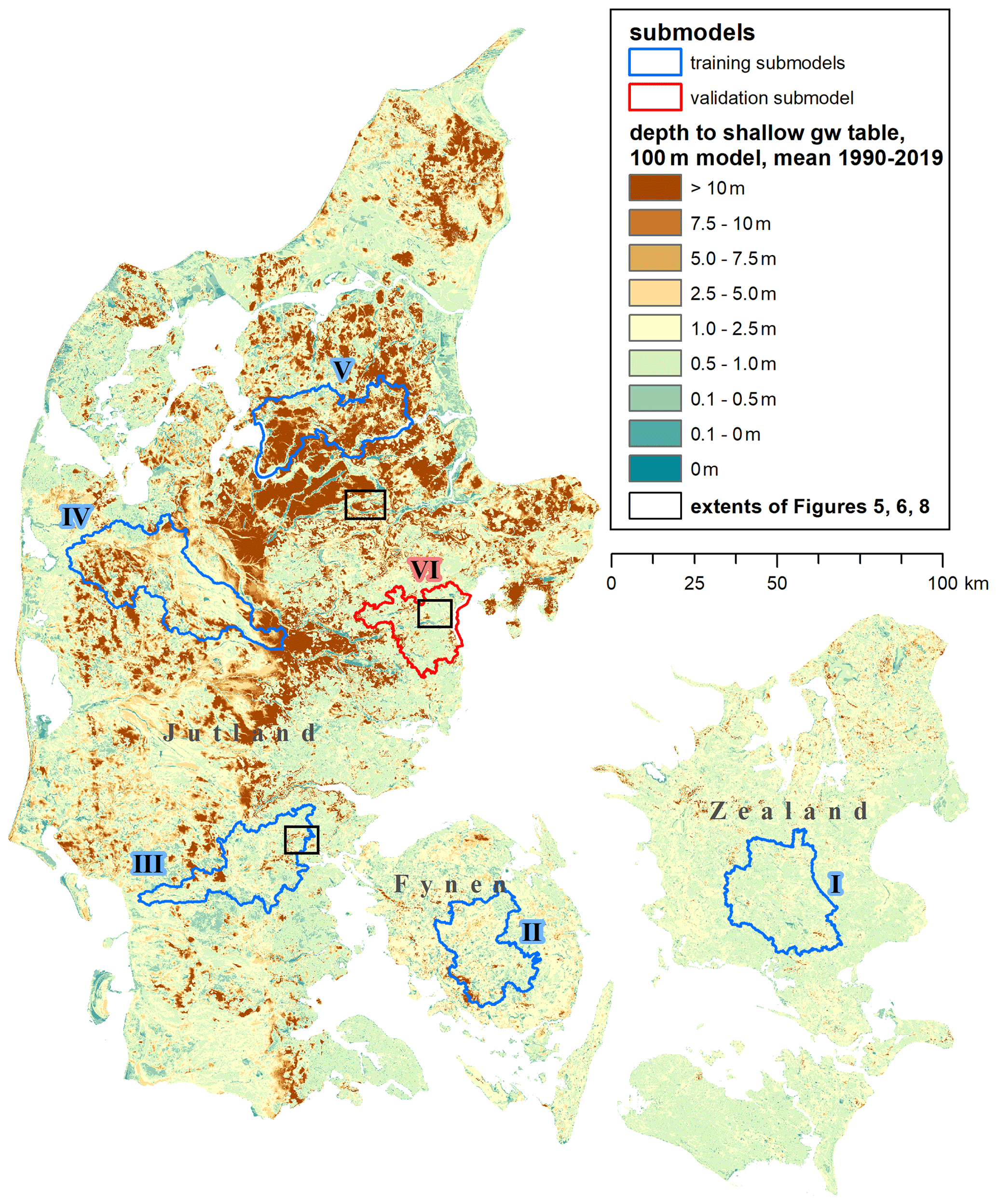
Figure 1 Denmark with the mean depth of the shallow groundwater table, as simulated by the DK-model HIP at a 100 m resolution for the period 1990–2019. The submodels used for training and validation of the downscaling algorithm are outlined in blue and red. The extents of the detail maps shown in Figs. 5, 6, and 8 are indicated as black rectangles.

This requirement for high-resolution data is particularly relevant when evaluating climate-change-induced impacts on the shallow groundwater table. The national water resource model of Denmark (the so-called DK-model) is based on a distributed, coupled surface–subsurface model at a 500 m horizontal resolution, and recently at a higher-resolution 100 m version with specific focus on surface-near processes. As forcing for climate change impact studies, a large ensemble of locally bias-corrected climate models is available (Pasten-Zapata et al., 2019). Ideally, national hydrological impact assessments would be based on the high-resolution version of the hydrological model (HM). However, the 25-fold increase in computational nodes for the 100 m model compared to the 500 m model makes such a modelling task infeasible due to the computational burden.

In order to obtain national impact projections at high resolution based on a large climate ensemble, but with a minimized computational cost, it is proposed to develop a downscaling method based on machine learning (ML) to refine impact simulations from the computationally feasible 500 m HM to a resolution of 100 m.

Within other fields such as remote sensing, ML-based spatial downscaling algorithms have been explored and used for several years, for example in the DisALEXI modelling system (Anderson et al., 2004, 2021). Here, the background is often to bridge gaps between coarse-resolution imagery from some satellites that typically have a frequent revisit time, and high-resolution imagery from other satellites with lower temporal resolution (Yang et al., 2017; Im et al., 2016). Moreover, image-sharpening techniques that build scale-independent models are utilized to increase the spatial resolution of satellite data (Guzinski and Nieto, 2019). Similarly, spatial downscaling is widely applied for weather predictions and climate models (e.g. Cheng et al., 2020; Sun and Tang, 2020). We hypothesize that applying similar techniques on outputs from complex HMs, combining the information of physically based models with various high-resolution spatial data and ML methods will increase relevance of HM outputs. This is a relatively new field with a few applications so far. For example, Koch et al. (2021) used HM outputs as covariates in ML algorithms predicting groundwater table depth at high spatial resolution, or Zhang et al. (2021) downscaled GRACE total water storage data with the help of HM output from the Global Land Data Assimilation System (GLDAS). Here, the presented research is contributing to the further integration of physically based HMs with ML techniques. This can also contribute to the discussion of further development of knowledge-guided or theory-informed ML techniques in hydrological science (Nearing et al., 2021).

Hence, the objective of this work is to develop a ML-based algorithm for spatial downscaling of physically based HM outputs. This is applied to the downscaling of climate change impact predictions on the simulated depth of the shallow groundwater table for Denmark, downscaling from a resolution of 500 to 100 m. We favour an ML-based approach over simple interpolation methods or topography-driven downscaling, because ML has the capability to effectively learn multivariate relationships which we expect to be highly relevant for a complex variable like the shallow groundwater table. Even though running the DK-model nationwide at the fine 100 m resolution with a full ensemble of climate models is computationally too expensive, it is feasible to run some selected submodels at a 100 m resolution and utilize their high resolution outputs as training data for the ML-based downscaling. In addition, a single national-scale deterministic run with historic climate is possible at 100 m, which can serve as valuable information to the downscaling algorithm. Also, all the relevant model input data are available at a resolution of at least 100 m.

2 Data and methods

2.1 DK-model HIP

The national water resource model for Denmark, the DK-model, covers most of the Danish land surface area of approximately 43 000 km². It has been developed continuously over several decades (Højberg et al., 2013; Henriksen et al., 2003; Stisen et al., 2019) and has been used in various research projects (recent examples: Koch and Schneider, 2022; Noorduijn et al., 2021; Schneider et al., 2022; Soltani et al., 2021), public consultancy as well as in relation to the EU Water Framework Directive. It targets, for example, questions of water resource availability, water quality, and future impacts on the hydrological cycle due to climate and land use change. Most versions of the DK-model have a horizontal resolution of 500 m, while a version at 100 m horizontal resolution was created as part of the Danish Hydrologic Information and Prognosis system (HIP; Henriksen et al., 2020b). This most recent version, hereafter referred to as DK-model HIP, is the basis of the presented work. Figure 1 displays mean historic depths of the shallow groundwater table as simulated by the DK-model HIP: Shallow groundwater levels are within the first 1–2 m from the surface for large parts of the country, with variations mostly controlled by topography and geology.

The importance of the location of the shallow groundwater table, and it being controlled by small-scale variations in topography and geology, is also one of the main motivations for the creation of the finer 100 m resolution DK-model HIP (see also the 10 m resolution map of average groundwater tables developed in the same project by Koch et al., 2021).

2.1.1 General hydrological model setup in MIKE SHE

The DK-model HIP is an integrated, distributed surface water–groundwater model setup in the MIKE SHE model code (Abbott et al., 1986; DHI, 2020). MIKE SHE is used to couple 3D subsurface flow, 2D overland flow, a simple two-layer description of the unsaturated zone, and 1D kinematic routing of flow in the stream network. It is run as a transient model with daily climate forcing and a maximum time step of 24 h.

The description of the DK-model is kept short here, as the model itself and its development is not the focus of this paper. For more details on model setup, input, and parameterization, the readers are referred to the provided literature in the following two sections.

2.1.2 Input data and conceptualization

The DK-model HIP exists in two distinct horizontal resolutions of 500 and 100 m, with all relevant input data available at 100 m resolution. The saturated zone is divided into 9–11 computational layers of varying thickness, depending on the region. The 3D unit-based parameterization of the subsurface is based on a nationwide hydrogeological model, with the exception of the uppermost computational layer with a constant thickness of 2 m which is parameterized based on the Danish soil map (Jakobsen et al., 2015).

Human water use is included to the extent that groundwater extractions for drinking water and irrigation are included; sewage plant outflows are also added to the model. Moreover, the model includes a representation of (subsurface) drainage, which is widespread in Denmark (as described in Schneider et al., 2022).

As historic climate forcing for precipitation, temperature, and potential evapotranspiration, the gridded, daily data from the Danish Meteorological Institute is used (Scharling, 1999a, b). Temperature and potential evapotranspiration are provided at 20 km resolution and precipitation at 10 km, and interpolated to the respective HM resolution of 100 or 500 m. Daily precipitation is corrected as described by Stisen et al. (2011).

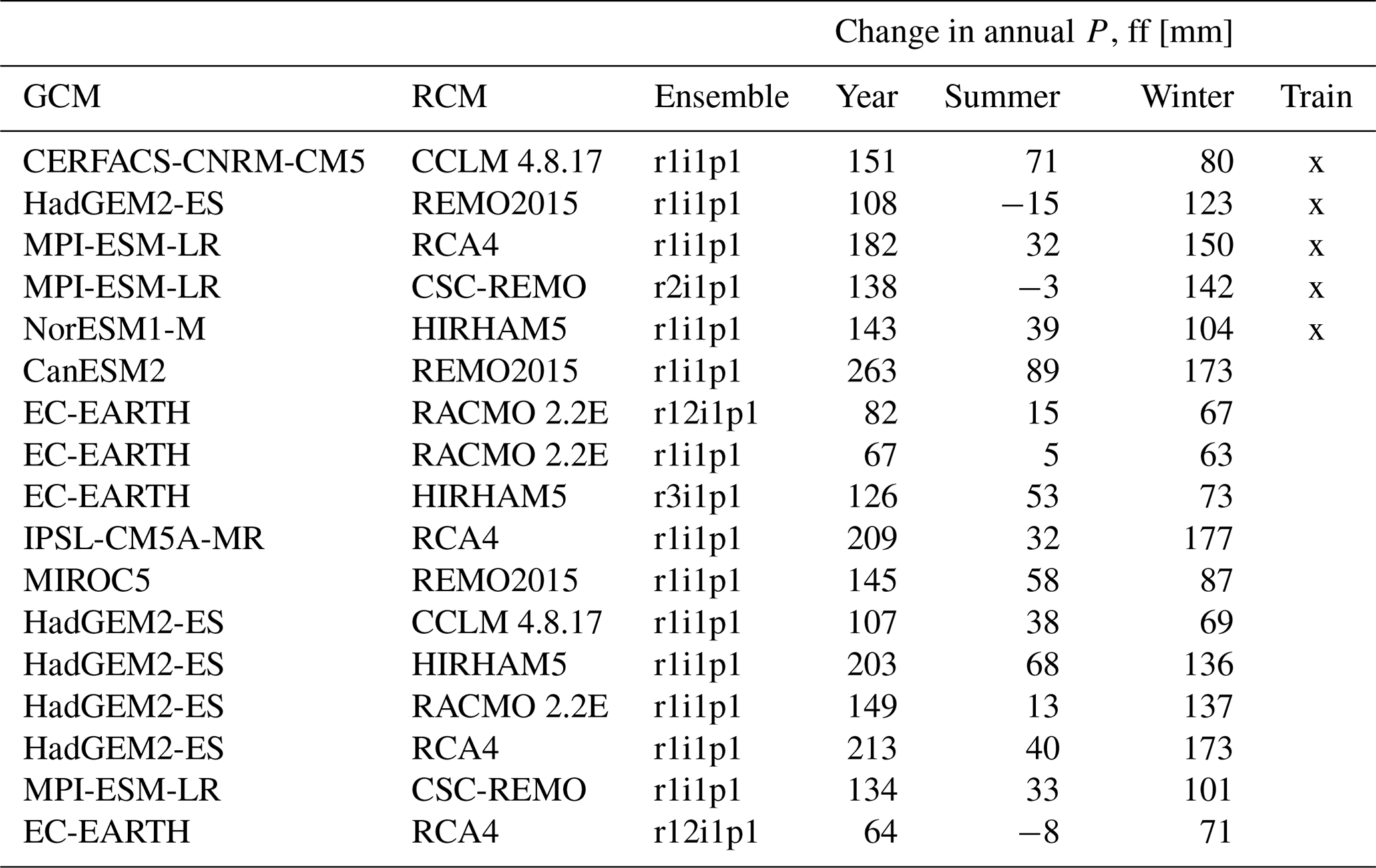
Table 1 Overview over the 17 used bias-corrected RCMs. The training models are marked. Changes to projected precipitation (P) are given for the far future (ff) relative to the reference period, yearly as well as separately for the summer and winter half year.

2.1.3 Model calibration

The national DK-model HIP was calibrated in its 500 m version, against observations of groundwater heads and streamflow for the period 2000 to 2010, and validated from 1990 to 1999 and 2011 to 2019. For calibration, the model optimization tool PEST (Doherty, 2015) was used with its implementation of the Gauss–Marquardt–Levenberg algorithm. Again, due to excessive computational effort, it was not possible to conduct such a calibration, requiring a large number of model runs, with the full 100 m national model. However, through a validation comparison, it was deemed feasible to directly transfer the calibrated parameters from the 500 m version of the model to its 100 m version without loss of performance. On the contrary, especially the performance for shallow groundwater heads was improved moving from the 500 m to the 100 m version. A recalibration of a limited set of parameters for 10 subcatchments in 100 m yielded no substantial additional improvement in model performance. Details regarding the model calibration are beyond the scope of this paper and can be found in Henriksen et al. (2020a).

2.2 Input data for future climate scenarios

2.2.1 Climate models

An ensemble of regional climate models (RCMs) from the Euro-CORDEX initiative (Jacob et al., 2014) was used in this work. Those RCMs were locally bias corrected for Denmark and remapped to the same 10 and 20 km resolutions of the historical climate data as described in Pasten-Zapata et al. (2019). All RCMs cover the years 1971 to 2100 with daily time steps. For the work presented here, we used 17 RCMs representing the RCP8.5 greenhouse gas concentration scenario (van Vuuren et al., 2011) shown in Table 1. Out of that ensemble of 17 RCMs, we selected a subset of 5 RCMs. Those 5 RCMs were selected based on their ranges of projected precipitation, to cover a wide range of future climates, ensuring that the median precipitation predictions across the 5 selected RCMs are close to the median precipitation predictions of the entire ensemble of 17, as well as cover variances in changes between summer and winter precipitation. This subset of 5 RCMs was used with the 100 m submodels (Fig. 1), producing the training data for the downscaling.

2.2.2 Further input data for future scenarios

Besides climate forcing, some further input data were adapted to account for future conditions: sea level is included as fixed head boundaries along sea boundaries of the HM. For the historic model runs, the sea level is kept constant at an elevation of 0 m. For the future scenarios, sea-level rise was accounted for as projected by the Danish Meteorological Institute (Thejll et al., 2021).

Changes in groundwater abstraction rates, sewage plant outflows, and land use were not projected, but current historic values and maps were assumed for the future period. Irrigation is simulated demand driven in the model; hence, it automatically accounts for climatic changes.

2.3 Climate change impact runs with the hydrological models

An overview of the different climate change impact runs performed with the HMs is given in Table 2. Due to computational limitations, we ran the full ensemble of 17 RCMs with the 500 m national HM only (C; B is a subset of C). Besides that, we selected five training subcatchments, covering about 9 % of Denmark's surface area in total, and ran those with five selected RCMs at 100 m resolution (D). To allow for a fully independent validation, a sixth validation submodel was run at 100 m resolution, with the full RCM ensemble (E). Finally, the DK-model HIP was also run for all of Denmark with observed climate forcing, for the period 1990 to 2019. These historic runs were performed both at 500 and 100 m resolutions (A and *). Relevant HM outputs were initially stored at daily time steps and then aggregated as described below in Sect. 2.3.1.

Table 2 Overview of the performed HM runs with different climate inputs for Denmark and different submodels. A – used as covariate. B – to be downscaled, in training, and as additional training data (auxiliary points). C – to be downscaled, in validation. D – training data. E – validation data. ^*: Not directly used in this study.

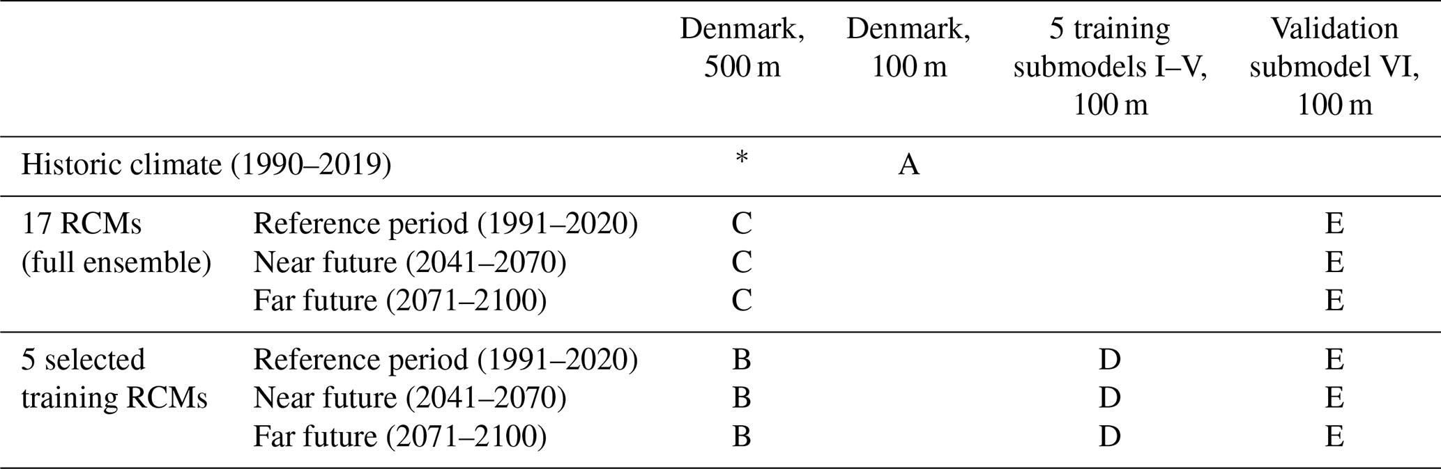
For the climate change impact evaluation, the HMs were run using each individual member of the ensemble of RCMs as forcing, for three different periods: the reference period, serving as baseline, as well as the near future period (nf), and the far future period (ff). For the reference period, model outputs were extracted from 1 January 1991 to 31 December 2020, for the near future from 1 January 2041 to 31 December 2070, and for the far future from 1 January 2071 to 31 December 2100. The HMs were started with initial conditions taken from a continuous run of the corresponding HM across the entire period of 1991 to 2100, using conditions from the same date as the respective simulation start. A warmup period of 4 years prior to the start dates for result extraction was allowed for each of the HM runs.

2.3.1 Climate-change-induced changes to the shallow groundwater table

Finally, the climate change impacts of interest were the average conditions across each of the future 30-year periods, subtracted from the reference 30-year period. These climate change impacts on the shallow groundwater table are hereafter also referred to as to-be-downscaled-variables (TBDVs).

That means we focus on changes to the groundwater table caused by future climate change, as opposed to absolute values, as changes can be more useful than absolute values when comparing present-day to future conditions. This is mostly because changes to the groundwater table are typically small compared to the absolute depth of the groundwater table and the uncertainties in the modelled absolute depth. Hence, when evaluating future conditions, an absolute value predicted by the HM can only be used in direct comparison to present-day output of the same HM. If being used in different contexts, for example in comparison with more detailed local HM results or observations of the groundwater table, the discrepancies between these absolute values will dominate and potentially mask the projected changes. When using predicted changes between reference and future period HM outputs with the same HM setup, those projected changes can be attributed with high confidence to the changes in climate.

Hence, we downscale projected climate-change-induced changes to the shallow groundwater table. Different aggregated statistics were chosen, and changes were calculated for both the nf and ff periods. The chosen aggregated statistics are the changes to the mean, 1st percentile, and 99th percentile of the simulated groundwater table (high and low groundwater tables, respectively), as well as changes to the 1 m exceedance probability. The latter represents the fraction of time the groundwater table is closer than 1 m to terrain during the given period. The 1 m threshold was chosen based on user feedback (Stisen et al., 2018), and is relevant due to issues with infrastructure and agriculture caused by high groundwater levels, many of which are expected to start if the groundwater is closer than 1 m to the surface (e.g. the typical depth of tile drains around 1 m). This results in a total of eight statistics to be downscaled (TBDV, see also Table 3). For example, the change to the 1st percentile depth of the groundwater table for the nf period Q01_nf g is calculated as

$$\begin{array}{}\text{(1)}& Q{\mathrm{01}}_{\mathrm{nf}\mathrm{g}}=\mathrm{median}(Q\mathrm{01}{\left({\mathrm{nf}}_i\right)}_{\mathrm{g}}-Q\mathrm{01}{\left({\mathrm{ref}}_i\right)}_{\mathrm{g}}),\end{array}$$

where Q01(nf_i)_g is the 1st percentile of depth of the groundwater table simulated in each of the HM's grid cells g individually, across all daily values of the 30-year nf period, and Q01(ref_i)_g is the respective value for the 30-year reference period; i refers to each of the individual members of the RCM ensemble used, and the actual TBDV is then the median change across the RCM ensemble. The subscript g is omitted in the following for ease of readability. In equivalent manner, all the eight TBDVs mean_nf, mean_ff, Q01_nf, Q01_ff, Q99_nf, Q99_ff, ex1m_nf, and ex1m_ff are calculated. Moreover, in the same manner as the TBDVs were calculated based on the 500 m national DK-model HIP outputs, the respective training data were calculated based on the 100 m submodels.

2.3.2 National climate change impact runs at 500 m

The full national DK-model HIP was run at 500 m resolution with the full ensemble of 17 RCMs (which includes the 5 selected training RCMs). This 500 m model output represents the data that are to be downscaled to the finer 100 m resolution with the presented method.

2.3.3 Submodel runs at 100 m

Six submodels distributed across Denmark (outlined and marked in Fig. 1), each representing a hydrologic subcatchment and setup at 100 m resolution, were chosen to produce training and validation data for the downscaling algorithm:

• I

  Suså

• II

  Odense Å

• III

  Kongeå/Kolding Å

• IV

  Storå

• V

  Simested Å/Mariager Fjord

• VI

  Aarhus Å/Aarhus (validation only)

The five submodels I to V were used as training data, whereas submodel VI was used as a fully independent validation dataset. To reduce computational effort spent on HMs, the five training models were run with the five selected RCMs, i.e. the training data are based on the reduced RCM ensemble. For the validation, to address the extrapolation capability of the downscaling algorithm, the validation model was also run with the full ensemble of 17 RCMs. The submodels were run with the same general model setup, periods, and warmup as for the national model described at the start of Sect. 2.3. Along the land boundaries of the submodels, dynamic boundary conditions were applied based on the simulated groundwater heads in the corresponding 500 m national HM.

The five training submodels, along with the sixth validation model, were deliberately selected to cover a representative range of geologic, topographic, and hydrologic variability occurring across Denmark. The ML methods are known to perform poorly when used to extrapolate data beyond the range of data they are trained against (Meyer and Pebesma, 2021). Figure 2 displays the histograms of one of the variables to be downscaled (TBDV), together with some important covariates. The values covered by the five training submodels closely resemble the distribution and ranges seen across all of Denmark; i.e. the submodels are considered representative of all of Denmark. Similarly, the validation submodel also covers comparable covariate ranges.

Table 3 Overview of the covariates.

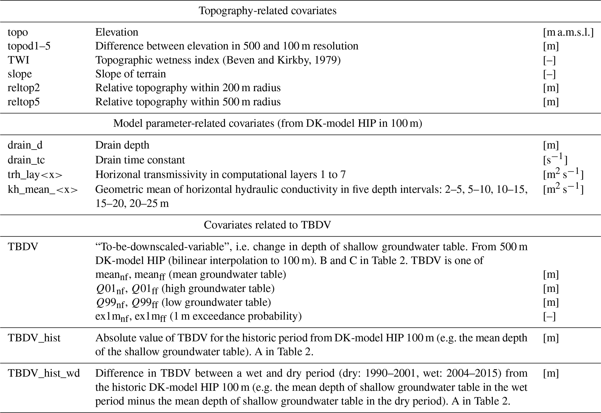
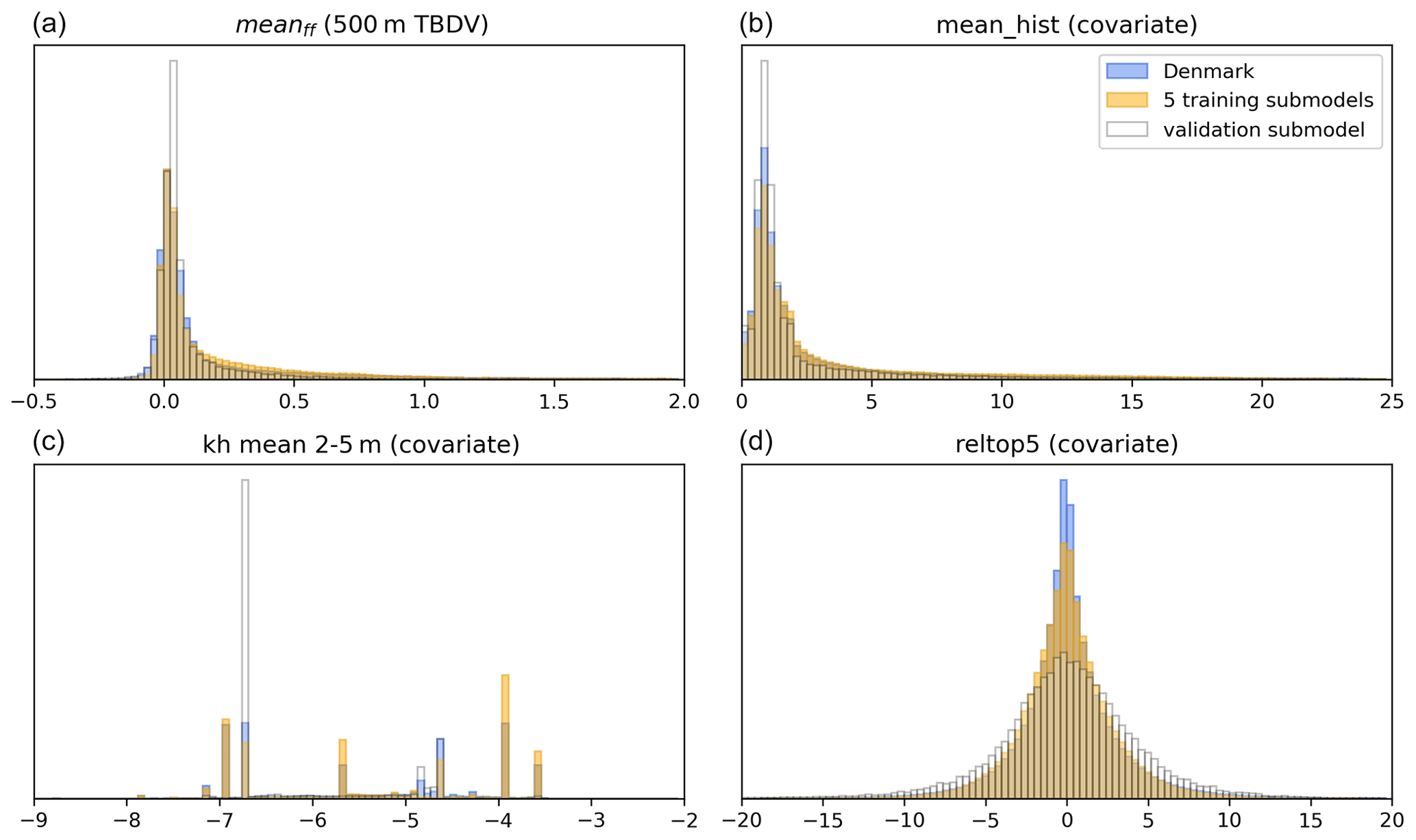
Figure 2 Histograms of covariate ranges covered by the five training and the validation submodels, compared to all of Denmark. Shown for the example of TBDV mean_ff. (a) Change in mean depth of shallow groundwater from the 500 m model (i.e. the TBDV) [m]. (b) Mean depth of shallow groundwater from the historic 100 m model (the respective most important covariate) [m]. (c, d): kh mean 2–5 m ([m s⁻¹], log-transformed) and reltop5 [m] as two more covariates.

2.4 ML-based downscaling

2.4.1 Covariates

Table 3 presents an overview of the covariates used in the downscaling algorithm. The first type of covariates is topography-related, and contains six different covariates. Secondly, 14 covariates derived from the DK-model HIP parameters were used: this group contains the horizontal transmissivities for the uppermost 7 computational layers of the model's saturated zone, and the mean horizontal hydraulic conductivities across 5 depth intervals, as well as the spatially distributed drain depths and drain-time constants used in the model. The last group contains the actual 500 m change to the groundwater table that is to be downscaled (the TBDV). Besides that, the respective absolute value corresponding to each TBDV from the 100 m historic HM is included. Furthermore, the differences in TBDVs between a historic dry and wet period were included. For the wet period, the 12 consecutive years between 2004 and 2015 were used (average yearly precipitation of 852 mm), and for the dry period, the years 1990 to 2001 were used (average yearly precipitation of 817 mm). The differences between wet and dry historic periods were calculated in the same manner as the changes between future and reference periods, and are assumed to be a proxy for expected changes with future, generally wetter, climates.

All covariates are available at the target resolution of 100 m for all of Denmark, to allow the application of the downscaling algorithm to the entire country. The only exception obviously is the TBDV itself, which is only available at 500 m nationwide. It was resampled from its native resolution to 100 m using bilinear interpolation: initial tests showed performance improvements of the downscaling algorithm if interpolated TBDVs were used; using resampled TBDVs without interpolation lead to visible artefacts at the 500 m grid boundaries in the 100 m outputs.

More covariates have been used in preliminary tests. Analyses of covariate importance and collinearity, excluding non-informative and strongly correlated covariates, lead to the final set of 23 covariates.

2.4.2 Random forest regressor

For the downscaling task at hand, we decided to use a random forest (RF) regressor. The RF goes back to Breiman (2001) and over time has proven to be a powerful and versatile data-driven modelling tool for a range of applications in environmental sciences. For example, RF was used in the context of groundwater pollution (Rodriguez-Galiano et al., 2014; Tesoriero et al., 2017), data analysis and predictions in large-sample hydrology (Addor et al., 2018; Ghiggi et al., 2019), as well as some of the remote-sensing downscaling models mentioned in Sect. 1. Examples from related Danish contexts include the prediction of groundwater level changes based on well observations (Gonzalez and Arsanjani, 2021), modelling of the historic depth of shallow groundwater and redox boundary (Koch et al., 2019b, a), or the modelling of artificial drainage properties (Motarjemi et al., 2021; Møller et al., 2018).

RF is a supervised ML method, requiring labelled training data. Based on the training dataset, an RF regressor model learns about relationships between a set of covariates and the target (training) data values. In the next step, predictions at unsampled locations beyond the training data can be made. Tyralis et al. (2019) provide a concise overview of the theory behind and the use of RF in hydrological contexts.

We used the implementation of RF regressors in Python 3.8 from the scikit-learn package, version 1.0.2 (https://scikit-learn.org/1.0/modules/generated/sklearn.ensemble.RandomForestRegressor.html?highlight=random forest regressor#sklearn.ensemble.RandomForestRegressor, last access: 17 November 2022).

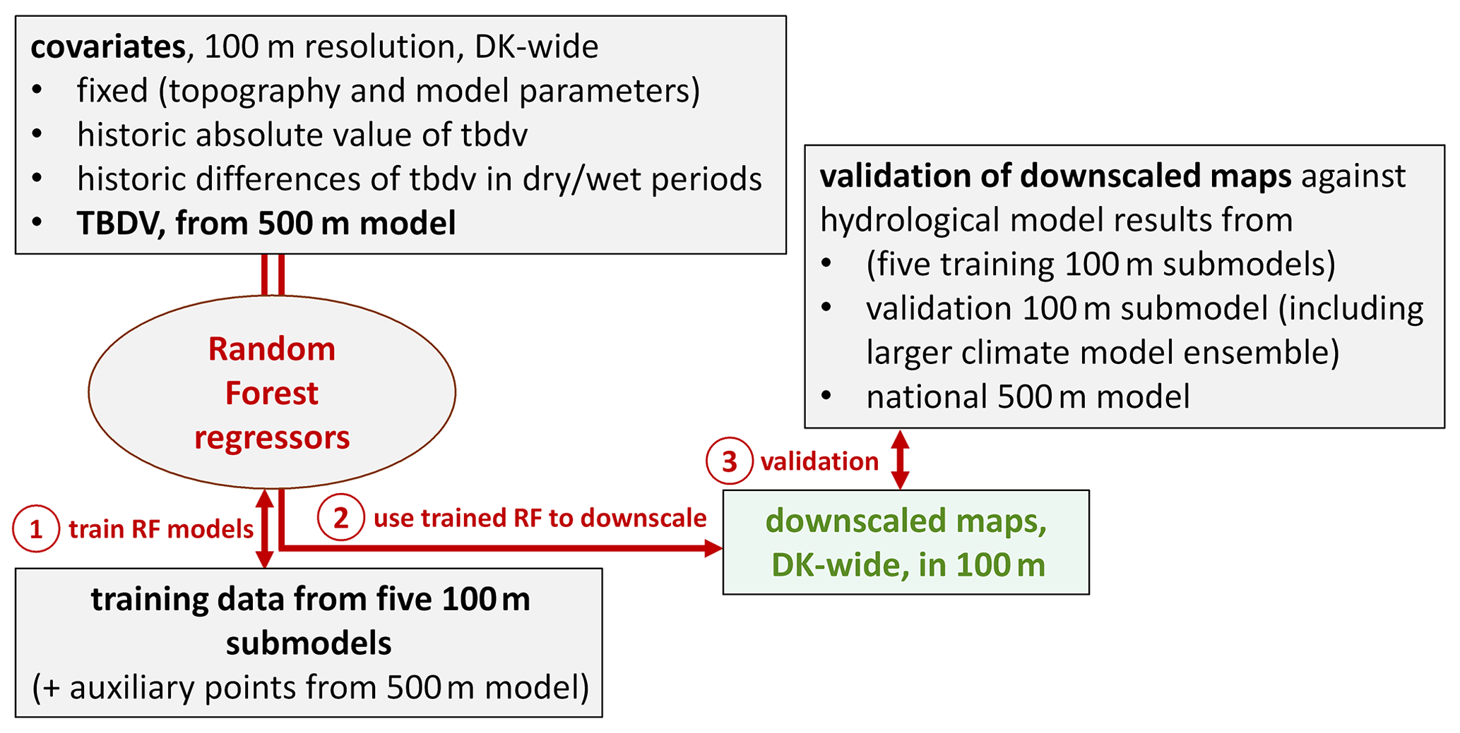
In Fig. 3, a workflow diagram of the downscaling algorithm is shown: all covariates exist at 100 m resolution for all of Denmark, with the exception of the actual TBDV, which originates from the 500 m HM. The TBDV exists at the finer target resolution of 100 m for the five training submodels – these data are used as training data for the RF downscaling regressors, alongside some auxiliary points from the 500 m HM (see below). After training, the RF regressors are used to produce Denmark-wide maps of the TBDV at 100 m. The downscaled outputs are validated against both national HM output, the training data, and a sixth, independent validation submodel at 100 m. Details are presented in the following sections.

Figure 3 Diagram of the downscaling algorithm.

2.4.3 Auxiliary points for RF training

Initial tests with spatial cross validations of the downscaling algorithm showed issues with the predictions for the spatial hold-out, i.e. with spatial transferability of the algorithm to areas not covered by the training data. To improve spatial transferability, it was decided to include additional training data sampled from the entirety of Denmark outside the training submodels, which enhance the spatially limited training dataset. These points were sampled randomly in space. The actual training target – the TBDV at 100 m – is lacking for those points, and instead the TBDV at 500 m was used as training target. Hence, we refer to these points as auxiliary points. The inclusion of such auxiliary points increases the robustness of the RF downscaling outside the training data areas; for example, we experienced some areas where the downscaling incorrectly reversed the direction of change to the groundwater table without using auxiliary points, which was alleviated after including auxiliary points. Despite the covariate ranges being adequately covered by the training catchments (Fig. 2), the auxiliary points still inform the algorithm by adding covariate values and likely combinations of covariates (the latter being a focus of the work on ML algorithm transferability by Meyer and Pebesma, 2021). However, the more auxiliary points are included, the closer the downscaled output resembles the original TBDV at 500 m, which is undesired. Considering this trade-off, we tested different amounts of auxiliary points, and settled on an optimal number of 20 000 auxiliary points covering all of Denmark to be included in the training data. This adds 5 % to the total number of data points in the training dataset comprised of the 5 training submodels, where all 100 m HM grids were included in the training data (approximately 400 000 points).

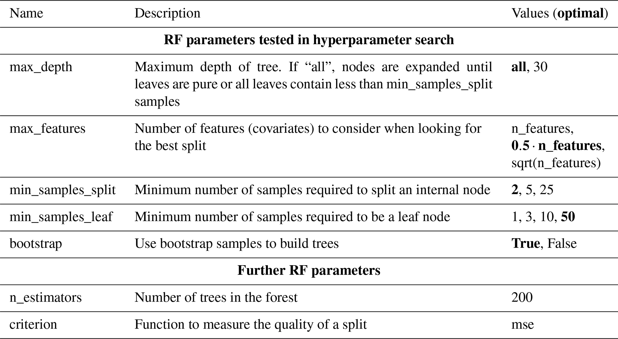
Table 4 The parameters used for the RF regressors. The first section presents the tested hyperparameters, where the selected values for each parameter are marked in bold. Further parameters are reported in the second section.

2.4.4 Training the RF regressors

The four different climate change impact statistics regarded in this work – i.e. changes to the depth of the groundwater table in average (mean), high (Q01), and low (Q99) conditions, as well as the probability of the groundwater table exceeding 1 m below terrain (ex1m) – are expected to be controlled by different properties. Hence, it was decided to train a separate RF downscaler for each of the four TBDVs. However, to ensure the consistency across near and far future and to increase the robustness of the downscaler by increasing the amount of training data, each of the downscalers was trained against data from both nf and ff periods simultaneously. That means that four RF downscaler models were trained; one for each mean, Q01, Q99, and ex1m.

The training was performed using the 100 m target values from the five fine-scale submodels (D in Table 2), based on the reduced RCM ensemble, as well as the auxiliary points from the 500 m HM. The respective TBDV at 500 m was taken from the national HM (B in Table 2). Beyond the training data at 100 m and the TBDV at 500 m, the other covariates presented in Table 3 were used.

Based on the training data, the importance of each of the covariates was evaluated: the information content (importance) that each covariate delivers to the RF regressors is determined by randomly perturbing each of the individual covariates one by one, retraining the model, and observing the decrease in model fit. Moreover, as covariate collinearity can lead to misleading results of such an analysis, the importance analysis was also performed by perturbing whole groups of related covariates at a time (e.g. Koch et al., 2019a).

2.4.5 RF hyperparameter search

Random forest regressors have built-in parameters controlling model behaviour and complexity, the so-called hyperparameters. To fine-tune and optimize the RF regressor performance, a hyperparameter search was performed using the standard grid-search procedure. The tested parameter values, resulting in 144 unique combinations, are listed in Table 4. For each of the parameter combinations, and each of the TBDVs, the following was performed:

• i

  An evaluation of the ability of the RF regressor to reproduce the 100 m HM results by determining Pearson's R was performed in a spatial cross-validation test, where the RF regressor was trained against four of the five training submodels. Its results were validated against the hold-out submodel, looping through all five permutations of train/hold-out submodels.

• ii

  An evaluation of the Denmark-wide bias introduced by the downscaling. Here, the RF regressor was trained against all five training submodels, and then used for predictions for all of Denmark. Those predictions were compared against the national 500 m HM results.

In this setup, (i) presents an indication of the RF regressor's ability to reproduce the fine-scale 100 m results, whereas (ii) represents an indication of the transferability and robustness of the RF regressor, with decreasing performance in the case of overfitting. Based on averaging these results across all TBDVs, a hyperparameter set representing an optimal trade-off was determined. These hyperparameters, marked bold in Table 4 alongside the other reported parameters, were then used in all subsequent tasks.

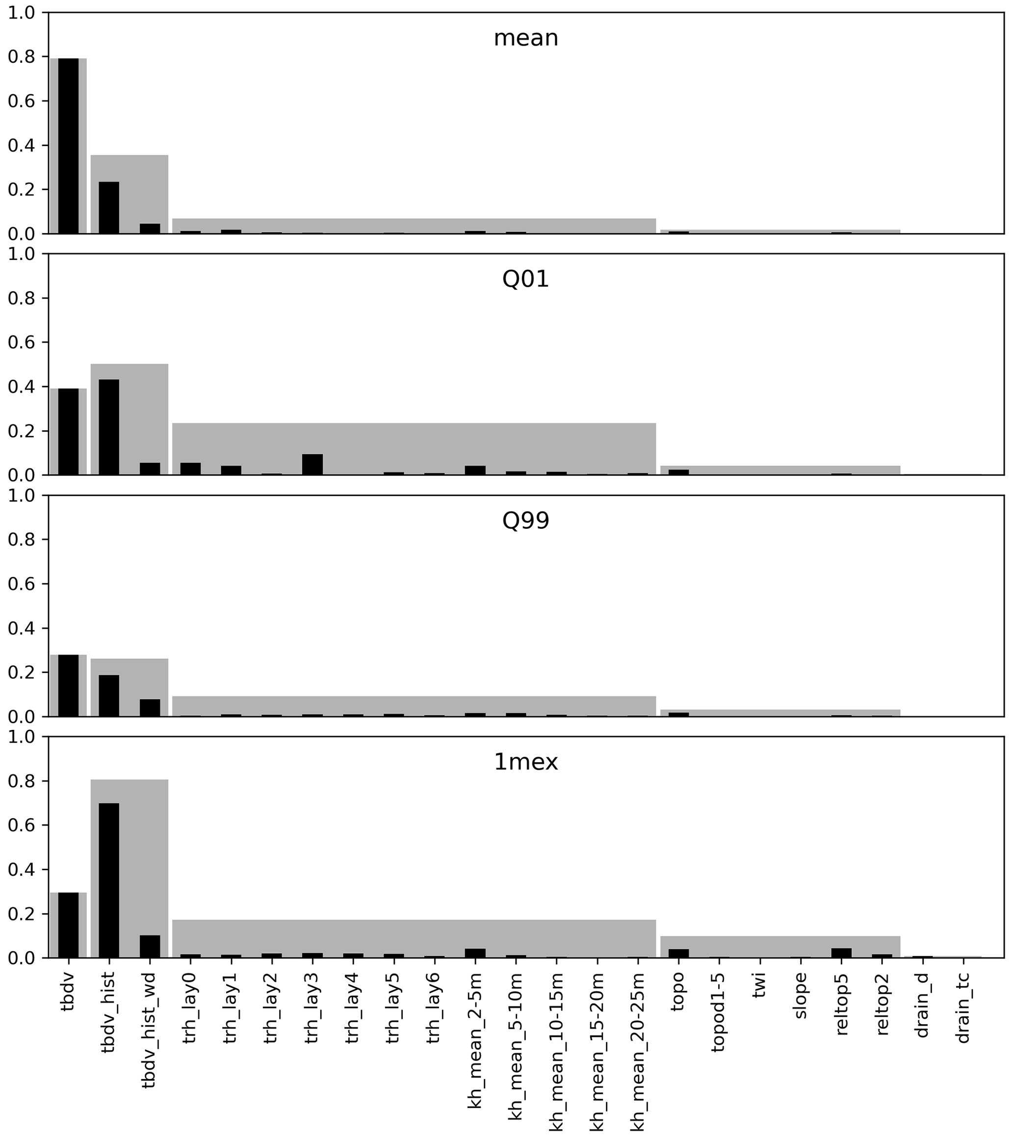
Figure 4 Permutation covariate importance for the four RF downscaling regressors, for each covariate (see Table 3 for an overview). The higher the reduction in R², the higher the importance of the covariate. Each importance is provided permuting one covariate at a time (black bars), and permuting whole groups of covariates (grey bars).

2.4.6 Validation of the RF regressors' downscaled outputs

Subsequent to training the RF regressors with the optimal hyperparameters, they were applied to produce predictions for the entirety of Denmark. That means that the four RF downscaler models were used to downscale the national 500 m HM outputs to 100 m, separately for both the nf and ff periods, and for both the ensemble of 5 RCMs used in the training as well as for the full ensemble of 17 RCMs. The only difference in downscaling for the different periods and RCM ensembles is in the used TBDV at 500 m, which always represents the corresponding period and RCM ensemble.

Validation of the downscaled results at 100 m was then performed in two distinct ways. First, against the national 500 m HM output, verifying that the downscaling does not introduce an overall bias. Second, against the 100 m HM output from the validation submodel VI, which was not used in the training process.

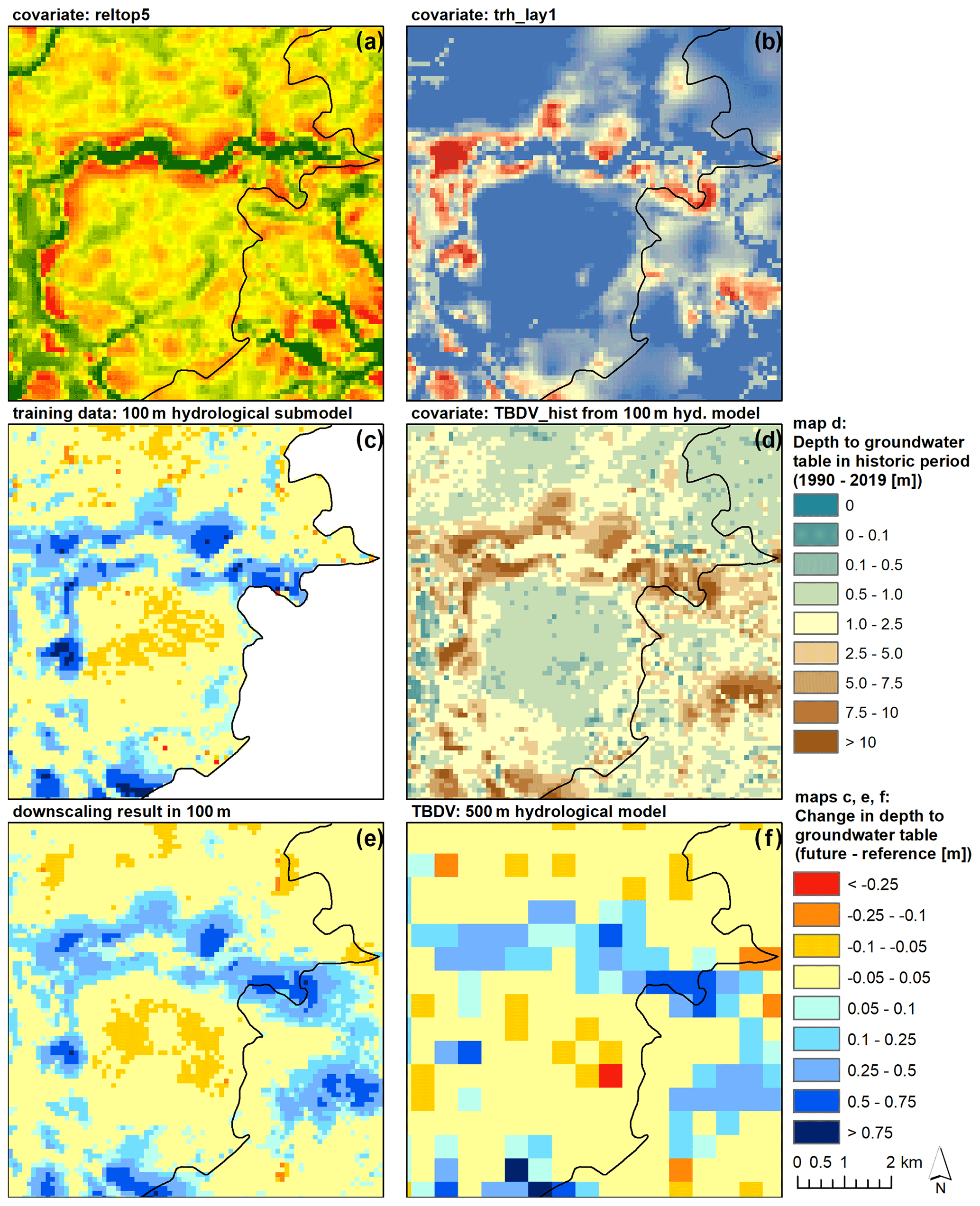
Figure 5 Example of downscaling results for changes to the mean depth of the groundwater table for the far future period (mean_ff). All panels show the same extent. (a, b) Examples for covariates (reltop5 and trh_lay1). (c) 100 m HM submodel results (training data). (d) 100 m historic absolute values (covariate). (e) 100 m downscaling result. (f) 500 m HM results (TBDV).

3 Results and discussion

3.1 Covariate importance

Figure 4 summarizes the results of the covariance importance analysis, for each of the final trained RF downscalers. Results are shown separately for individual covariate importance, as well as for covariate group importance. The groups in order of decreasing importance were as follows: (i) the TBDV itself, (ii) the historic TBDV from the 100 m model, (iii) the geology-related covariates, (iv) the topography-related covariates, and (v) the drain parameterization-related covariates. It is noteworthy that on average, the TBDV turns out as the most important covariate, followed by the respective historic absolute value of the TBDV and the difference between historic dry and wet periods. That means that the downscaling is largely guided by information on the TBDV itself, which is desired since our aim was to develop a downscaling algorithm. Turning to the topography-related and model parameter-related covariates, and comparing the different downscalers, it can be seen that Q01 (high groundwater tables) is more strongly guided by the hydraulic conductivities in the uppermost layers (the four most important covariates from that group being trh_lay0, trh_lay1, trh_lay3, and kh_mean_2–5 m). On the other hand, Q99 (low groundwater tables) is more guided by hydraulic conductivity from lower layers (the four most important covariates from that group being kh_mean_2–5 m, kh_ mean_5–10 m, trh_lay5, and try_lay1). In general, the topography-related covariates show a lower importance than the geology-related covariates, stressing the need for integrating geologic knowledge when modelling groundwater levels.

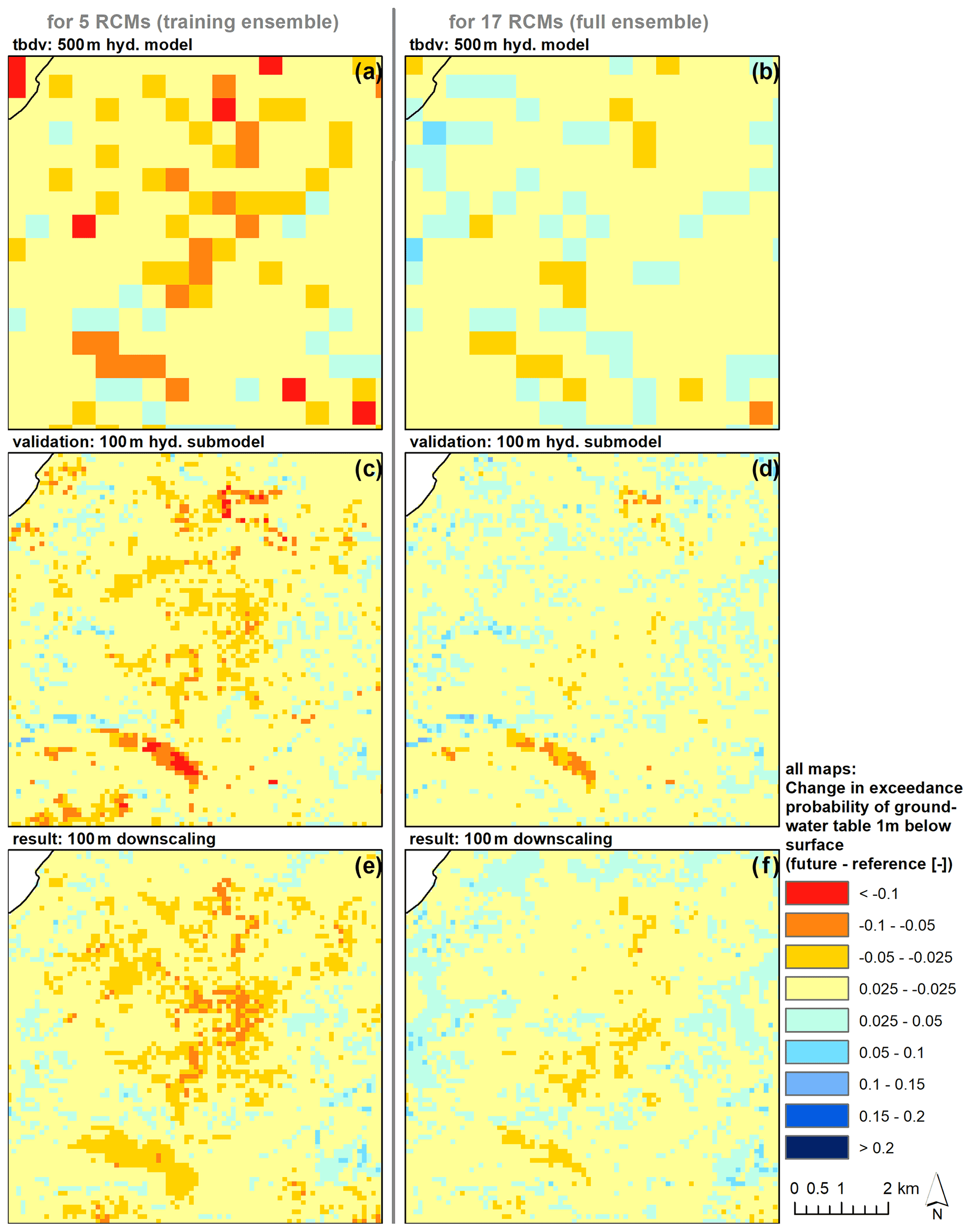
Figure 6 Downscaling outputs for validation submodel VI, for the example of ex1m_nf. Left column: The RF downscaling was trained to downscale the median change of the five RCMs from the 500 m HM (a) with the 100 m HM training data (c; however, submodel VI is not included in the training). Downscaling results are shown in (e). If applied for the full RCM ensemble (b, d, f), the downscaling results (f) also align with the truth (d).

3.2 Downscaled output

Figure 5 presents different input data and results for the same area located at the north-eastern edge of submodel III Kongeå/Kolding Å (extent indicated in Fig. 1), for the example TBDV mean_ff. The top row (panels (a) and (b)) shows examples for two of the used covariates, the relative topography, and the horizontal hydraulic transmissivity in the second layer of the HM. Panel (d) shows the simulated mean groundwater heads from the historic 100 m HM, which is used as a covariate. In panel (c), the used training data from the 100 m hydrological submodel can be seen, whereas panel (e) shows the corresponding downscaled result at 100 m resolution. Comparing those two panels, together with the actual TBDV in panel (f), i.e. the results from the HM at 500 m resolution, gives a good visual example of the capability of the downscaling algorithm to reproduce the details at 100 m resolution from the 500 m coarse-resolution input. It also emphasizes the value of the fine-scale information. As can be seen, the 100 m HM output resolves significant variations in both the absolute values of the depth of the groundwater table as well as the climate-change-induced changes to the groundwater table that are completely lost at 500 m resolution. The complexity of the fine-scale variations also goes beyond what can be achieved by merely interpolating the coarser 500 m to the finer 100 m resolution. Rather, it becomes apparent that local variations in groundwater levels and level changes are controlled by an interplay of topography and geology.

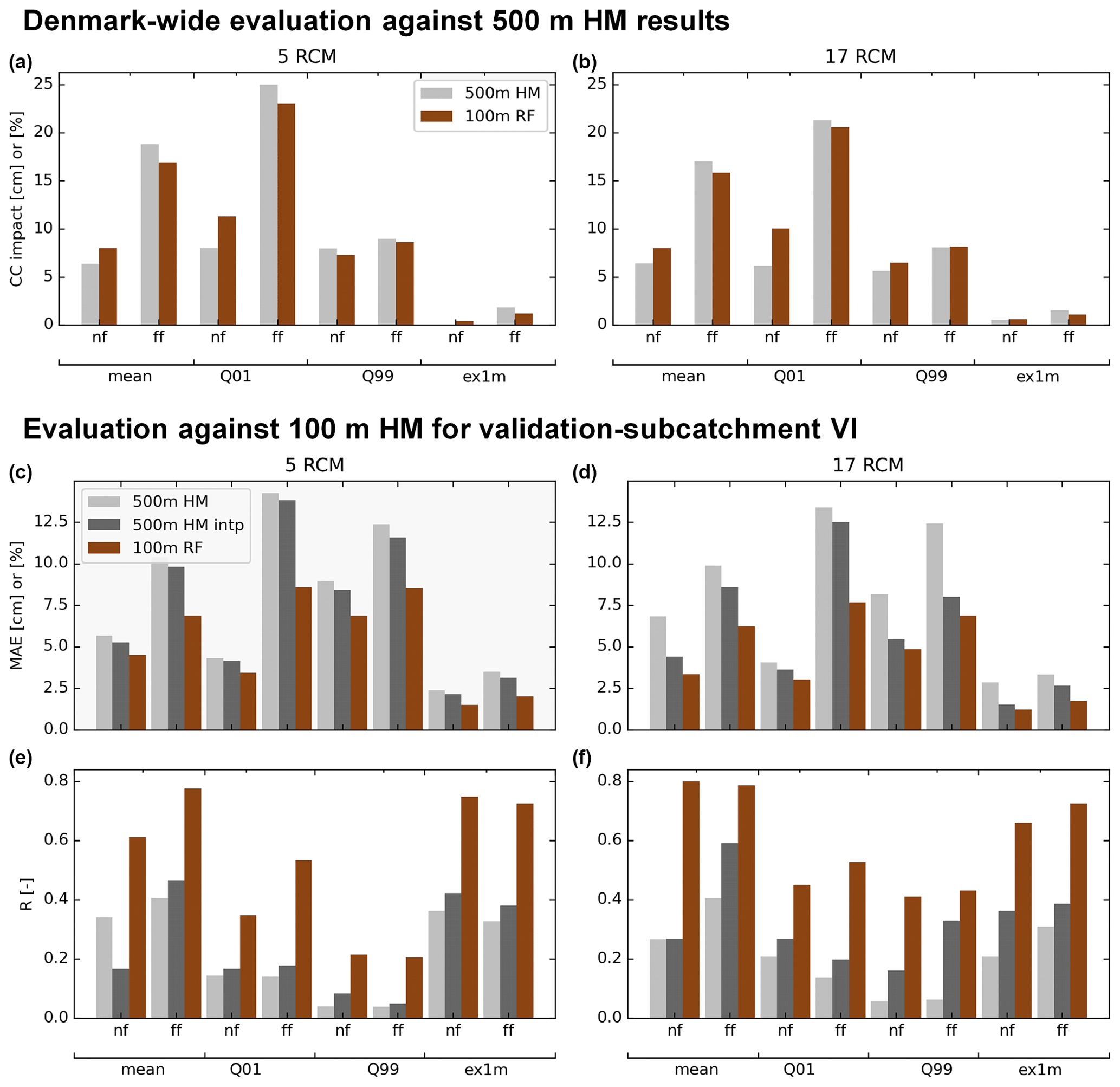
Figure 7 Overview of the validation results of the RF downscaling algorithm. (a, b) Climate change impact on the TBDV. (c, d, e, f) MAE and Pearson's R between the 100 m HM from the validation submodel and the corresponding 500 m HM, both in its original resolution and using bilinear interpolation to 100 m (“500 m HM intp”), as well as the 100 m RF results. Values along the y axis are given in cm for mean, Q01, and Q99, and in % for ex1m, for both near (nf, 2041–2070) and far future (ff, 2071–2100).

Figure 6 illustrates downscaling results for the fully independent validation submodel VI Aarhus Å/Aarhus (extent indicated in Fig. 1), for the example of TBDV ex1m_ff. The left column shows the median change of the five RCMs used in the training exercise, where the top row displays the TBDV from the 500 m HM (B in Table 2). The middle row shows the respective TBDV as simulated by the 100 m HM submodel (E in Table 2). The bottom row then displays the respective downscaling results in 100 m. The right column shows the corresponding results for the full RCM ensemble of 17 models. These 17 RCMs were not used in training, but only in validation. Even if confronted with a different climate signal (compare the differences between the 500 m HM outputs in panels (a) and (b) in Fig. 6), and used outside the area of training data, the downscaling algorithm still works well. That means it is robust enough to be trained based on a (small) RCM ensemble, and then be applied to HM output based on a different (larger) RCM ensemble, which is also in line with the findings from the covariate importance analysis, where the corresponding TBDV showed to be the most important covariate.

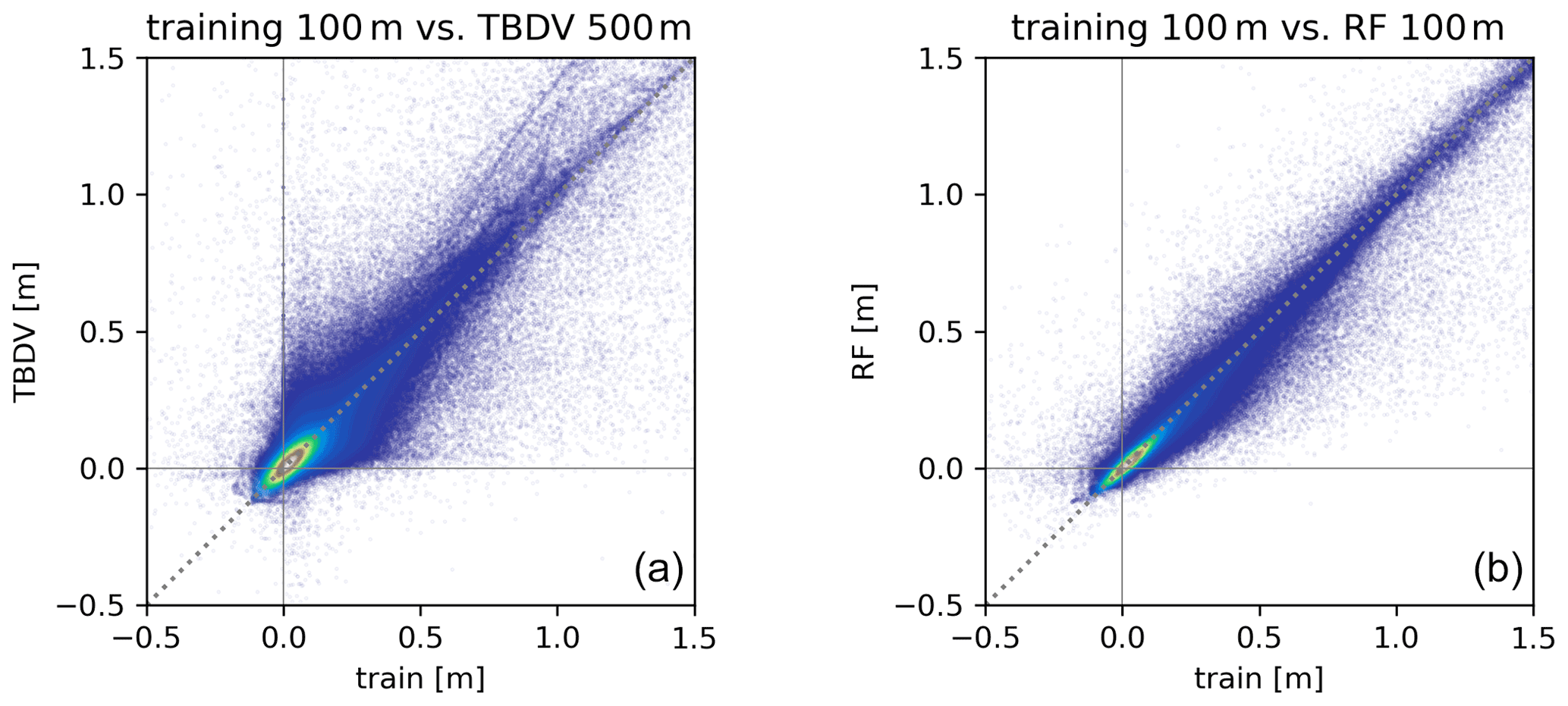
Figure 8 Scatterplots for the example of TBDV mean_ff: comparing the training data (i.e. the TBDV in 100 m) with the actual TBDV in 500 m (a), and with the RF downscaling results in 100 m (b) for the five training submodels.

These visual evaluations of the downscaling outputs can be confirmed quantitatively – Fig. 7 presents an overview. The top row presents a Denmark-wide evaluation of the climate-change-induced changes to the shallow groundwater table. The bars present the mean changes across all of Denmark for each of the eight TBDVs (i.e. mean, Q01, Q99, and 1mex for both near and far future), as predicted by the 500 m national HM runs, and the downscaled outputs in 100 m, respectively. It can be observed that generally, the downscaling does not introduce overall biases to the predicted changes, but remains true to the general picture predicted by the coarser national HM. This applies to both the ensemble of 5 RCMs, as well as the full RCM ensemble with 17 models. The bottom two rows of Fig. 7 display validation results of the downscaling output against 100 m HM outputs for submodel VI, i.e. this is a fully independent validation of the 100 m RF downscaling output versus 100 m HM outputs. Spatial transferability to independent areas without training data is a well-known weakness of the used ML techniques. However, our RF downscaling model proves to be robust also in this context: Pearson correlation coefficients between the 100 m RF output and the 100 m HM output are consistently higher than correlation coefficients between 500 m HM output and 100 m HM output. It can also be seen that the RF downscaling adds more information than a simple interpolation, as results are given separately for the 500 m HM outputs and a bilinear interpolation of the 500 m HM outputs. The latter is considered the benchmark to be beaten to determine whether a downscaling algorithm actually delivers additional information over the coarse-scale HM outputs. The same applies to the mean absolute error (MAE) between the 100 m RF downscaling output and the 100 HM, which is consistently smaller than the MAE between the 500 m HM and 100 m HM.

For the example of the TBDV mean_ff, per-pixel data are presented in scatterplots in Fig. 8. The left panel shows a comparison of the 100 m training data from the HM of the five training submodels against the corresponding TBDV from the 500 m HM. Most values range between roughly −10 and 30 cm, which means that the mean groundwater table for the far future period is predicted to mostly be between 10 cm lower to 30 cm higher than in the reference period. There is good general agreement between the 500 and 100 m HMs and no general bias, but a considerable scatter caused by the differences in resolution. This is in line with the previously discussed lack of bias in the predicted changes from the 500 and 100 m HMs as apparent from the top row of Fig. 7. The right panel shows a comparison of the 100 m training data and the RF downscaling predictions in 100 m. Here it can be seen that the downscaled results follow the 100 m HM outputs more closely than the 500 m HM outputs, with a much narrower scatter.

Finally, Fig. 9 displays Denmark-wide results of the downscaling algorithm, for all four TBDVs of the far future period mean_ff, Q01_ff, Q99_ff, and ex1m_ff. Each of the detailed maps shows the same extent: they serve as a good illustration that groundwater tables (and changes to them) are controlled by small-scale landscape features, such as topography and geology. If only 500 m information was available, many details would be lost that are apparent in the 100 m resolution. For many purposes, e.g. agriculture, information on the groundwater table at the coarse scale of 500 m is inappropriate – a grid size of 25 ha is larger than typical field size. However, with a resolution of 100 m, i.e. 1 ha, we move into more relevant, near-field-size resolutions. Furthermore, as the downscaled outputs are still based on physically based HMs, fine-scale physical information is added on the interplay of controls such as topography and geology on the groundwater table.

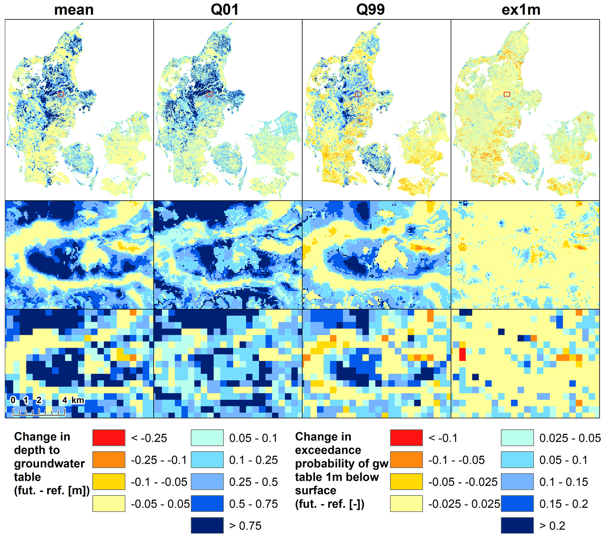
Figure 9 Results of the downscaling, for the far future of all four TBDVs. Top row: Downscaling results in 100 m for all of Denmark. Middle row: Detail of the 100 m downscaling results (extent indicated in top row). Bottom row: Same detail for the corresponding TBDV in 500 m.

Moreover, Fig. 9 also displays the initially mentioned tendency to more extreme groundwater levels: the low groundwater tables (Q99), typically occurring during the summer months, are projected to fall across many regions of the country, especially across Zealand and southern Jutland where groundwater levels are very shallow and affected by evapotranspiration. The high groundwater tables (Q01), typically occurring during the wetter winter months, are simulated to rise further for most of the country. Some of the highest rises are simulated for areas in central Jutland where the shallow groundwater levels are deep below surface (compare Fig. 1). Moderate rises are also simulated in regions where the groundwater tables are very shallow (within the first 1 or 2 m below surface), such as parts of Zealand and Funen.

3.3 Overarching discussion

Despite the discussed capabilities of ML techniques in exploiting large datasets at high spatial resolution, physically based HMs are still needed to predict climate-change-induced changes to the hydrological cycle. Purely data-driven methods (often based on ML algorithms) struggle with predicting previously unobserved states, which holds true for both spatial and temporal extrapolation (Meyer and Pebesma, 2021; Mai et al., 2021; Koch and Schneider, 2022). As an attempt to overcome the computational burden of high-resolution, complex HMs, Tran et al. (2021) have developed an ML-based emulator of an HM. Read et al. (2019) and Koch and Schneider (2022) showed that guiding ML models with simulation data from a physically based model enhanced the capability of the ML model to extrapolate. The downscaling algorithm presented in this work increases the resolution of HM outputs, guided by fine-resolution HM outputs.

As our method is based on output from distributed, physically based HMs, we (i) are able to obtain fully distributed climate change impact evaluations, and (ii) have higher confidence in extrapolating the models to values outside observed ranges, which is unique and, for example, goes beyond recent efforts with purely data-driven extrapolations of climate change impacts on groundwater levels for selected wells across Germany (Wunsch et al., 2022). Our developed downscaling algorithms were shown to be robust, transferrable in space, and also transferrable to a different climate signal, i.e. transferable to a different RCM ensemble.

Acknowledging computational limitations, we based our 100 m training data on five HM subcatchments, representing around 9 % of Denmark, which were run with forcings from a reduced ensemble of five RCMs. This meant that the computational time for hydrological model runs was reduced to less than 3 % of what would be required for a nation-wide full ensemble run at 100 m. The size of the training dataset was chosen to be sufficiently large to allow for extrapolation beyond the area of the training data. We also assume that the careful choice of the training submodels, covering a variety of different hydrogeological settings across Denmark, facilitated the spatial transferability of the downscaling algorithm. For other applications of similar downscaling algorithms, the necessary size of the training data also depends on the specific application – an algorithm used for predictions to a limited area or within the training data requires a smaller training dataset than an algorithm used for extrapolation beyond areas with training data.

The downscaling was facilitated by the consistency of parameter sets between the 500 and 100 m HM setups: we do not intend to compensate for potential discrepancies in simulated groundwater heads due to differences in parameter values, but merely want to downscale the 500 m national HM results to a finer scale as simulated by the corresponding model in higher resolution. The same applies for all the other input data: for both 100 and 500 m HMs, the same input data were being used, with the only exception of scale.

4 Conclusions

We successfully designed and tested an RF-based spatial downscaling algorithm for outputs from distributed HMs. The usage of ML techniques in spatial downscaling is widespread in fields such as remote sensing, however, still limited in hydrologic modelling. The developed downscaling algorithm is based on the existence of a coarse-scale HM for the full domain of interest, together with equivalent fine-scale HMs for limited parts of the domain. Furthermore, covariates in fine scale are required for the full domain. We trained the RF regressor based on the selected, representative fine-scale HMs covering only around 9 % of the full domain, significantly reducing computational effort on the complex HMs. Furthermore, using the downscaling algorithm in the context of an ensemble of RCMs, we could show that it is possible to train the downscaling algorithm based on a smaller ensemble of RCMs, and apply it to the full ensemble, further reducing computational effort on HMs. The downscaling results were successfully validated against the output from a fully independent fine-scale validation HM, as well as the full-domain results of the coarse-scale HM.

The presented framework is envisioned to be transferrable to the downscaling of other spatial output from hydrological and environmental models in general, also beyond aggregated statistics (i.e. also in transient manner). It is generally acknowledged that there is a disparity between the – computationally possible – spatial resolution of HM output, and what is desired or required by users of the data, such as authorities, consultants or citizens (Samaniego et al., 2019). Also from a scientific point of view, we are commonly dealing with HM resolution issues and spatial aggregation beyond what is appropriate, hindering process understanding (Wood et al., 2011; Nijzink et al., 2016).

This also applies to the greater context of this paper, the Danish HIP4Plus project (Henriksen et al., 2020b). Within this project, a larger dataset of climate-change-induced changes to the shallow groundwater table was generated based on the presented framework. This includes predictions for different greenhouse gas concentration scenarios (RCP4.5 and RCP8.5), further statistics, and monthly as well as seasonally aggregated values; a total of 236 variables (as compared to the 8 presented here). All downscaled maps and further data can be accessed via the HIP data portal https://hip.dataforsyningen.dk/ (last access: 17 November 2022). Due to computational limits, the spatial resolution of HMs is, in many cases as in the presented example, below what is requested by end-users and decision makers. Downscaling can help to bridge the gap to make HM output more relevant, in this case within the context of climate change impact evaluation and adaptation, to deliver valuable input to urban and infrastructure planning, or agriculture and future needs for artificial drainage or water pollution risks.