Technical note: Modeling spatial fields of extreme precipitation – a hierarchical Bayesian approach

We introduce a hierarchical Bayesian model for the spatial distribution of rainfall corresponding to an extreme event of a specified duration that could be used with regional hydrologic models to perform a regional hydrologic risk analysis. An extreme event is defined if any gaging site in the watershed experiences an annual maximum rainfall event and the spatial field of rainfall at all sites corresponding to that occurrence is modeled. Applications to data from New York City demonstrate the effectiveness of the model for providing spatial scenarios that could be used for simulating loadings into the urban drainage system. Insights as to the homogeneity in spatial rainfall and its implications for modeling are provided by considering partial pooling in the hierarchical Bayesian framework.

1 Introduction

For an existing urban drainage network, a proper consideration of the spatial structure of extreme rainfall events is important for an assessment of the effectiveness of the network for handling urban flooding subsequent to rainfall events of varying duration, especially as concerns regarding the resilience of the system under a changing climate emerge. Often, investigators focus on return period analysis of extreme rainfall at a site considering annual maxima or peaks over threshold for a specific rainfall duration. In a regional context, spatial models of annual maximum rainfall are sometimes considered (Renard et al., 2006; Renard and Lang, 2007; Dyrrdal et al., 2015). However, since the annual maximum is unlikely to occur for a given event at all sites, these models do not represent the actual structure of potential extreme rainfall events. Thus, existing models for spatial rainfall extremes cannot be used to provide forcing for the performance of an existing drainage network (natural or constructed) under an extreme rainfall event. We address this situation in this note by considering that the rainfall events of interest for a specified duration are ones where any one of the sites in the region experiences an annual maximum event; the spatial field or rainfall of interest is then the field associated with each such event.

In the exploratory analyses performed for New York City, we noted that the structure of storms that lead to annual maximum events at different gages in the region may not be the same and that the basic statistics of rainfall vary across sites. We assemble a dataset of the annual maximum rainfall for each specified duration at each station. Let us denote this as A_djt for duration d, site j, and year t. These events may not occur on the same day of each year across the stations. Second, we consider the rainfall field at all stations associated with the annual maximum at any one station and call this the “spatial field” (SF), R_djki, where i is identified as an event such that R_dkki=A_dkt for site k=j for year t. R_djki then has the rainfall at all sites j for the event where site k has an annual maximum. As a result, the total number of events, i, may be much larger than the total number of years of data, N. A spatial event field of rainfall is thus conditional on the occurrence of an annual maximum rainfall for any station. Of interest is f(R_djki|A_dkt)f(A_dkt), where f(.|.) and f(.) refer to a conditional and marginal probability distribution, respectively. For example, in 1979, the annual maximum 12 h rainfall for the Central Park rainfall gage was 3.29 inches. At this time of the day, eight other rainfall stations around New York City had 12 h rainfall accumulations of 1.70 inches (Essex Fells), 2 inches (JF Kennedy International Airport), 2.73 inches (LaGuardia Airport), 0.79 inches (Newark International Airport), 1.68 inches (New Brunswick), 0.67 inches (New Milford), 0.98 inches (Staten Island), and 0.87 inches (Watchung), respectively. However, not all of those other accumulations were annual maximum events in their respective sites. Hence, A_12-CP-1979= 3.29 inches, and R_12-j-CP-i= [3.29, 1.70, 2.00, 2.73, 0.79, 1.68, 0.67, 0.98, 0.87]. This is similar to the issue noted by Asquith and Famiglietti (2000). See Table A1 in the Appendix for a full example of the spatial rainfall fields in 1979. The hierarchical Bayesian models developed consider the spatial field SF with the goal of providing an approach for stochastically generating representative spatial fields of rainfall for a specified duration, such that at least one site in the region experiences an annual maximum event. This is fundamentally different from the traditional rainfall frequency analysis which models annual maximum data at each site independently or using a covariance structure from the annual maximum data at all sites. In this paper, we formulated and tested a simple model that could directly explore whether or not and to what extent there was opportunity to pool regional information on extreme rainfall events to describe plausible spatial fields of extreme rainfall.

In Sect. 2, we present the data and the context for the application to the greater New York area. In Sect. 3, we describe the details of the multivariate hierarchical Bayesian models. The results are discussed in Sect. 4. Finally, in Sect. 5, we present a summary and conclusions.

2 Data description

2.1 Greater New York area context

The greater New York City area has a high density of man-made infrastructure and hence a complex hydrological landscape. Like many older cities, sanitary and industrial wastewater, rainwater, and street runoff are collected in the same sewers and conveyed together to treatment plants. Approximately 60 % of NYC's drainage area is served by these combined sewers. Flooding and combined sewer overflows (CSOs) are a concern, and innovative solutions for using the sewer system itself as flood storage by pumping water to different areas during a storm has been suggested. Such hydrologic system upgrades need to be informed by the spatial variability of extreme precipitation.

There are very few rain gage records that are longer than 20 or 30 years. Persistent data quality issues further reduce the available data. This challenge of reconciling sparse data with spatially variable hydrological networks and meteorological phenomena is common to many urban areas. Widely accepted design standards are derived from a set of intensity–duration–frequency curves developed using daily rainfall records from the period 1903–1951 (The New York City Department of Environmental Protection, 2008). An analysis of precipitation extremes for the region is offered in Wilks and Cember (1993), using daily rainfall data, and in McKay and Wilks (1995), using hourly rainfall data. None of these analyses consider the spatial correlation of rainfall.

2.2 Precipitation data

The precipitation data was obtained from the National Climatic Data Center (National Climate Data Center, 2013). Rain gages were selected based on their proximity to New York City, data quality, and length of the historical record. Twenty-nine stations were initially identified as lying within a 100-mile radius of Central Park, with over 25 years of continuous hourly rainfall records. Sixteen stations were excluded, since the resulting data quality was too poor. The final dataset consists of the remaining nine stations (Table 1); abbreviations for each station used in the figures throughout are provided in the first column.

Table 1 Rain gage stations in New York City and surroundings.

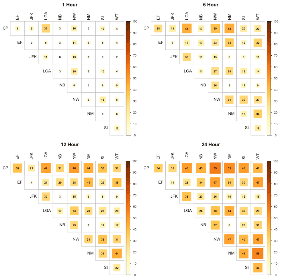
Figure 1 Percent of simultaneous or near-simultaneous annual maxima events shown for the site-by-site comparison for nine sites and 1, 6, 12, and 24 h storms.

2.3 Diagnostics and spatial concordance

The Shapiro–Wilks test (Shapiro and Wilk, 1965; Royston, 1992) was applied to the log-transformed annual maxima series at each station for each storm duration from 1 to 24 h. For these 216 time series, the null hypothesis of the appropriateness of the log-normal distribution was not rejected for 98 % of the sites at the 1 % level, 88 % at the 5 % level, and 81 % at the 10 % level. Though other distributions – such as the generalized extreme value (GEV), Pearson, and log-Pearson type III (LP3) – are popular for extreme precipitation modeling, in our application to the spatial field of rainfall, only one of the sites experiences the annual maximum event, and others may not be extreme values. In such a setting, the log-normal distribution can often be an appropriate representation (Raiford et al., 2007), as seen here. Consequently, to illustrate the idea, we consider a log-normal distribution with spatial correlation across the sites for the NYC example. Other choices could very well be made.

A heat map showing the fraction of annual maximums that occur simultaneously is provided in Fig. 1. For these plots, we define simultaneous storms to be those beginning within ±n hours of each other (where n is a multiple of the event duration) to allow for the movement of a storm event over the area and to identify distinct, independent rainfall events. We see that precipitation extremes, even within a relatively local area, are frequently not simultaneous. As expected, the simultaneous fraction of concurrent area increases as the storm duration increases. However, even for a 24 h duration, less than 60 % of the events are concurrent. This is true even for the four closest stations – JFK, LGA, Central Park, and Staten Island – that are typically used to inform hydrologic design in New York City.

This diagnostic analysis highlights the importance of considering the spatial structure of extreme rainfall for an event with a specified duration.

3 Methodology

A hierarchical Bayesian approach that provides the ability to partially pool model parameters across the rain gage sites was developed. Full pooling would imply that a parameter (e.g., the mean or variance of the distribution) was homogeneous across the sites. No pooling would imply that each site was independent. Partial pooling is an intermediate step that allows information to be shared across sites at a level informed by the data. This results in a multi-level model, where model parameters are estimated at each site but are assumed to be drawn from the parameters of distributions that are specified at the regional level for each parameter (Gelman and Hill, 2007). Such an approach has been implemented for hydrometeorological extremes in Lima and Lall (2010) and in Kwon et al. (2008), and for paleoclimate reconstructions by Devineni et al. (2013).

3.1 Spatial fields hierarchical model conditioned on the site experiencing an annual maximum

In this model, we consider a conditional process – where site k has experienced an annual maximum event – and the corresponding rainfall amounts R_djki at all sites are observed. The logarithm of rainfall is considered to be normally distributed, and a multivariate normal distribution is specified for each site k where an annual maximum has occurred. For each such condition, we consider partial pooling of the mean rainfall across all sites and consider the spatial covariance across sites. We consider that the spatial field of rainfall may actually be different depending on which site experiences an annual maximum. The hierarchical model is described as below:

$$\begin{array}{}\text{(1)}& \begin{array}{rl}& {\mathbf{Y}}_k\sim \mathrm{MVN}\left({\mathit{\mu }}_k{\mathbf{\Sigma }}_k\right)\\ & {\mathit{\mu }}_{kj}\sim N\left({\mathit{\omega }}_k,{\mathit{\sigma }}_k^{\mathrm{2}}\right)\\ & \text{Priors}\\ & {\mathbf{\Sigma }}_k\sim \text{Inv-Wishart}(\mathbf{\Delta },\mathit{\nu })\\ & {\mathit{\omega }}_k\sim N\left(\mathrm{0},\mathrm{1000}\right)\\ & {\mathit{\sigma }}_k^{\mathrm{2}}\sim U\left(\mathrm{0},\mathrm{100}\right).\end{array}\end{array}$$

Y_k is the log of the rainfall field R_djki across all sites corresponding to when station k has an annual maximum. For the New York City application, it is a matrix of 64 (years) by 9 (stations) for a given duration and station k. Y_k is assumed to follow a multivariate normal distribution, with a vector of station means μ_k and covariance across stations specified by a 9-by-9 matrix Σ_k. At the second level of the model, the station-specific means μ_j are assumed to be normally distributed, with a common mean ω_k and variance ${\mathit{\sigma }}_k^{\mathrm{2}}$. This is a partial pooling approach with no covariates, as outlined in Gelman and Hill (2007). A non-informative conjugate prior, the inverse-Wishart distribution, is assumed for Σ_k, where Δ is the scale matrix and ν is the degrees of freedom (Gelman et al., 2004). If Σ_k is a j-by-j matrix, we assume ν equivalent to (j+1) and Δ equal to the j-by-j identity matrix (I). This is equivalent to a uniform prior on each variance element of the correlation matrix (Gelman and Hill, 2007). We give ${\mathit{\sigma }}_k^{\mathrm{2}}$ a non-informative uniform prior and ω_k a non-informative conjugate normal prior for computational convenience (Gelman and Hill, 2007; Gelman et al. 2004).

There are nine stations, and therefore there are nine distinct datasets Y_k and nine distinct models for each storm duration. For extreme rainfall events, i.e., those that exceed a nominal design return period, we outline a simulation strategy from these models that pools simulated fields that represent regional extreme events together.

3.2 Spatial fields single-level model

We consider a subset of the previous model where the assumption that the mean log rainfall drawn from a common spatial mean is relaxed. This leads to the simpler, no-pooling model represented below:

$$\begin{array}{}\text{(2)}& \begin{array}{rl}& {\mathbf{Y}}_k\sim \mathrm{MVN}({\mathit{\mu }}_{ks},{\mathbf{\Sigma }}_{\mathbf{ks}})\\ & {\mathit{\mu }}_{kjs}\sim N\left(\mathrm{0},\mathrm{1000}\right)\\ & {\mathbf{\Sigma }}_{ks}\sim \text{Inv-Wishart}(\mathbf{\Delta },v).\end{array}\end{array}$$

As in the hierarchical model, Y_k is the log of the SF when station k is at an annual maximum. The vector of precipitation means across j stations (including station k) is μ_ks, with a subscript s to indicate single-level model.

3.3 Spatial fields simulation for a regional T-year return period

The spatial fields model can be used to simulate rainfall fields corresponding to an annual maximum occurring at any one of the sites, k. Next, if we are interested in design rainfall fields represented by the T-year return period across the domain, we follow a two-step process. First, based on the model that is fit, we identify the T-year return period annual maximum rainfall event for each site, k. Then, from simulations of the multivariate rainfall fields using the model, we identify all cases where the rainfall at site k exceeds the T-year event for that site and take the corresponding simulated rainfall field across all sites, j. The process is outlined below:

• i.

  Threshold calculation. For each return period (T) and rainfall duration (D), a precipitation threshold is computed for each station using the posterior mean and variance from the station k's hierarchical Bayesian model. The threshold was computed using frequency factors K for the normal distribution (Guo, 2006) and the equation below:

  $$\begin{array}{}\text{(3)}& \log \left(Y_{T,dk}\right)=\stackrel{\mathrm{̃}}{{\mathit{\mu }}_k}+K\left(T\right)\ast \stackrel{\mathrm{̃}}{{\mathrm{\Sigma }}_{kk}}.\end{array}$$

  For example, letting k= 1 for Central Park, we compute the SF model from Y₁. We extract μ₁₁, the Central Park mean, and Σ₁₁, the Central Park variance, and use them in Eq. (3) above.

• ii.

  Simulate multivariate field for Y_k. From the hierarchical Bayesian model defined in Eq. (1), we simulate a large number of realizations M (e.g., equal to 10 000) of the rainfall fields Y_k corresponding to the case when site k has an annual maximum. These are based on draws from the posterior distributions of the parameters, and hence, they incorporate a consideration of parameter uncertainty.

• iii.

  Extract subset of simulations that exceed the T-Year event at site k. Retain a subfield Z_k from Y_k, such that Y_dkkm > Y_T,dk and that m= 1 … M is the index of the simulation.

• iv.

  Pool the T-year return period fields. The Z_k are subsamples of rainfall fields from each of the nine models, such that an equal number of draws from each of the k fields is selected. For T= 100 years, on average, 100 such samples will be generated from each station for M= 10 000, and 900 total fields are then available for our application to the New York City data for design or reliability analyses. For our illustrations here, we sampled the same number of fields that are obtained from applying steps (i) to (iv) on the observed rainfall fields data. In essence, the spatial fields corresponding to a T-year return period event are first derived from observed rainfall fields data; these T-year return period spatial rainfall fields then form the baseline to which the simulated T-year return period spatial rainfall fields derived from the posterior runs of the hierarchical model are compared. Note that, since there may be multiple sites with annual maxima per event i in the original R_djki data, and since these are contained in each random field indexed by k, and since we modeled this spatial field, the concurrence of high rainfall at those sites will also be reproduced in the simulations. Similarly, the incidence of high rainfall at multiple stations will also be correctly reproduced across the pooled data across the K simulations.

3.4 Model fitting and convergence

Two hundred and sixteen models (one for each duration and each site) were fitted using JAGS (Just Another Gibbs Sampler) (Plummer, 2003; Denwood et al., 2016). It uses a Markov chain Monte Carlo (MCMC) simulation algorithm (a Gibbs Sampler for the current example) to simulate the posterior probability distribution of parameters. A random normal distribution was used for the vector of station means (μ, μ_k, μ_ks), and a random Wishart distribution was used for the precision. Similarly, a non-informative conjugate normal prior for ω_k and a non-informative uniform prior for ${\mathit{\sigma }}_k^{\mathrm{2}}$ are assumed. In JAGS, the normal distribution is parameterized in terms of precision instead of covariance ($\mathbf{\Sigma },{\mathbf{\Sigma }}_k,{\mathbf{\Sigma }}_{\mathbf{ks}}$), as is noted by convention in the model formulas above. We simulated four chains, ran the model for 20 000 iterations, and the first half of the simulations were discarded as burn-in.

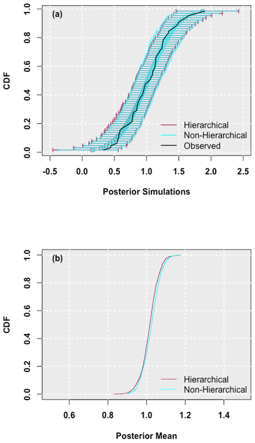
Figure 2 Empirical cumulative distribution function of the posterior distribution of (a) simulations and (b) mean parameters for the Central Park 12 h hierarchical and non-hierarchical SF model. Posterior means and simulations are shown on an untransformed scale (i.e., the mean is the log mean). The empirical cumulative distribution function derived from the observed data is also shown in panel (a) along with the band that depicts the 99 % credible interval of the posterior simulations.

4 Results and analysis

4.1 Bayesian model checking

For each model, the convergence of the posterior distribution of each parameter was checked using the shrink factor proposed by Gelman and Rubin (1992) – values under 1.1 for all parameters suggest that the model has converged. Convergence plots (showing the mixing of the four chains) were visually checked for all cases. All models converged appropriately, with each parameter attaining a shrink factor between 1.0 and 1.1 and with the large majority reaching 1.0.

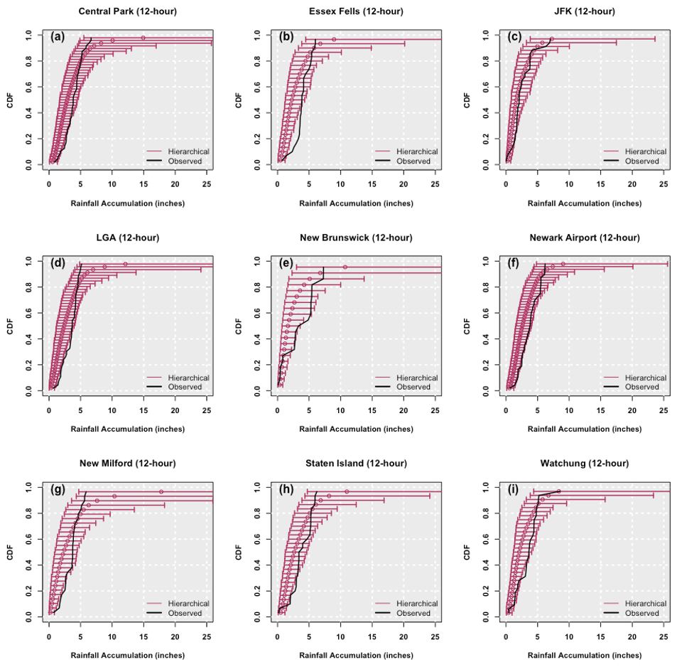
Figure 3 Empirical cumulative distribution function of the 12 h 10-year return period event from SF hierarchical models for the nine stations (Central Park, LGA, New Milford – top to bottom, left panel; Essex Fells, New Brunswick, Staten Island – top to bottom, middle panel; JFK, Newark, Watchung – top to bottom, right panel). The empirical cumulative distribution function derived from the observed 12 h 10-year return period field is also shown. The band depicts the 99 % credible interval of the posterior simulations.

We compare the performance of the two SF models using the deviance information criterion (DIC) and pD, as recommended in Gelman et al. (2004). The scores were virtually identical for the two types of SF models for each rainfall duration. Next, we considered whether the common mean in the hierarchical model converged as successfully as other parameters; it did. Gelman and Hill (2007) suggest that, when there are only a small number of groups and when the group-level standard deviation is large, multi-level modeling may not add much information. The resulting model will not necessarily perform worse and will likely resemble the model without pooling (as it does here). The posterior parameters for the resulting simulations are essentially identical (Fig. 2a), and the posterior for the mean shrunk only very slightly (Fig. 2b).

Figure 4 Empirical cumulative distribution function of 5-year return period events for 1 h (a), 6 h (b), 12 h (c), and 24 h (d) storms from Staten Island SF hierarchical model simulations. The empirical cumulative distribution function of the observed 5-year return period event fields at the respective durations are also shown. The band depicts the 99 % credible interval of the posterior simulations.

Next, we consider how the return period spatial rainfall fields identified in the SF hierarchical models compare to observed return period spatial fields. We do so by plotting the empirical cumulative distribution function of the return period event field estimated from the hierarchical model and by comparing it with the empirical cumulative distribution function of the return period event field derived from the observed data. The 99 % credible interval obtained from the posterior simulations of the hierarchical models is also presented to represent the uncertainty. Though the Bayesian models can easily simulate any return period, the reliability of the empirical estimate is dependent on the length of the record, so it is only reliable as a goodness-of-fit measure for shorter return periods. Results from all nine stations for the 10-year 12 h accumulated rainfall are presented in Fig. 3. The plots for all nine stations at the 1 and 24 h durations and the 10-year return period are provided in Figs. A1 and A2, respectively, of the appendix.

The observed 10-year 12 h return period fields for all stations are within the 99 % credible interval of the simulations, for the most part. The SF model simulated tails that are much greater in magnitude than the observed, as expected. The uncertainty band is also wider at the tail end of the distribution. New Milford is an exception, with slight underprediction of the left tail. These differences are amplified at the left tail for higher durations (i.e., the 24 h storms). The shorter durations (1 h storms) seem to be modeled well, albeit with wider credible intervals.

Figure 4 presents a slightly different view of the results, with a focus on how well various durations for a shorter return period event (5-year events) are simulated for a specific station – Staten Island. While 1 h 5-year return period storm fields are well simulated, there seems to be a bias (with the observed field's left tail falling outside the 99 % credible interval of the simulated) with increasing durations. It is difficult to identify exactly why this might be the case without significant additional exploratory analysis of the Staten Island data. However, we note that the simulations reflect additional information provided by the other stations in the model. In this application, the Staten Island site record is 20 years shorter than the record at the other sites, and the shift in the simulations reflects the shift in the rainfall in the other sites over this period. Thus, the pooling strategy is instrumental in using the joint distribution across sites from the common period of record to provide simulations that cover the shift in the period. Of course, if the correlation across sites has also changed over the period of missing data, the algorithm is incapable of replicating such a change.

5 Summary and conclusions

For larger cities, a consideration of the drainage network and the spatial dependence in rainfall at different durations is important to consider, at least from the perspective of assessing the performance and resilience of the network and perhaps also for design considerations. We were interested in formulating and testing a simple model that could directly explore whether or not and to what extent there was opportunity to pool regional information on extreme rainfall events to describe plausible spatial fields of extreme rainfall. This led to postulating and testing a Bayesian model that considers the spatial field of rainfall associated with an annual maximum occurrence at any site. We considered the application of the model to relatively long rainfall time series from the New York City region. Initial exploratory analyses suggested that the rainfall characteristics and storm tracks varied by event and by season across the region, such that distinct clusters could be identified, suggesting that the region had a heterogeneous spatial structure with respect to extreme rainfall (Hamidi et al., 2017). Our applications further clarified the nature of this heterogeneity. It is interesting to also note from the New York City analysis that there is support for pooling the spatial covariance of rainfall across all sites (irrespective of which one experienced an annual maximum rain event for a given duration), even though, often, the exceedance probability distributions of rainfall for a given duration may differ across sites, even after partial pooling. The hierarchical Bayesian framework permits a consideration of the uncertainty in parameter and model structure and helps us to identify the level of homogeneity that may be appropriate for representing the processes underlying a particular dataset.

Rain gages are the preferred data source for extreme event modeling because of their long record, but incorporating radar in addition to rain gages could provide the spatial density needed to explore how event rainfall characteristics relate to specific meteorological phenomena or to provide comparable simulations to existing stochastic models. The radar information would contain considerably more spatial detail necessary for building the type of model exemplified here. However, radar rainfall records are much shorter, and consequently, one needs to develop a methodology to appropriately blend the shorter but spatially richer radar data with the longer but spatially sparse gage data. Our algorithm can be readily applied to a mix of radar and rain gage data. However, some extensions need to be pursued to address the very different record lengths of each data source.

We used a log-normal distribution applied to rainfall for each duration to illustrate our approach. The goodness-of-fit tests support this assumption, and this permits some confidence in the kind of conclusions we drew from the applications to the New York City data. However, other models – such as the GEV or generalized Pareto or other choices for the distribution – could very well be considered. The point here was to highlight the need to consider spatial covariance and an appropriate blending of local and regional data sources through partial pooling.

Appendix A: Auxiliary figures

This appendix includes Table A1 and Figs. A1 and A2. Table A1 provides an example derivation of extreme rainfall fields. Figures A1 and A2 provide the results and baseline comparisons of the 1 and 24 h 10-year return period events from the SF models for the nine stations in and around New York City.

Table A1 Illustration of spatial rainfall fields for an example year, 1979, for 12 h accumulated rainfall. Anchor station column is the condition where annual maximum rainfall is identified (A_dkt). The corresponding row presents the rainfall for other stations when the anchor station is experiencing an annual maximum event (R_djki|A_dkt). For instance, the third row shows the spatial rainfall field when JF Kennedy International Airport had an annual maximum event in 1979 (2.03 inches of 12 h rainfall is shown in bold font to indicate the annual maximum rainfall at the conditioning station). The 12 h rainfall recorded at the other stations simultaneously are presented across, in the row. Notice that none of those other stations' recorded rainfall is the at-site annual maximum event.

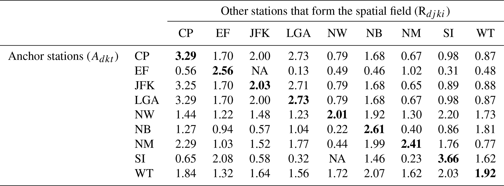
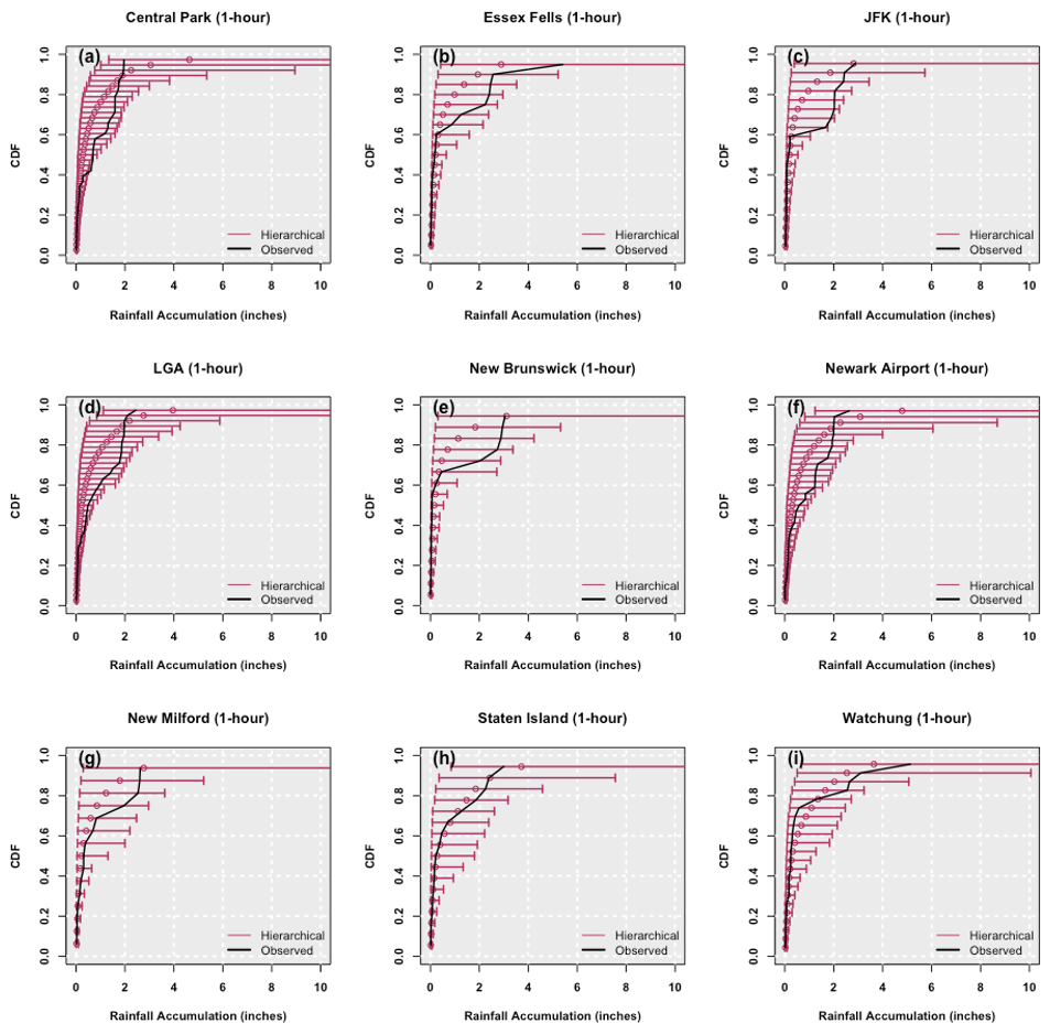
Figure A1 Empirical cumulative distribution function of the 1 h 10-year return period event from SF hierarchical models for the nine stations (Central Park, LGA, New Milford – top to bottom, left panel; Essex Fells, New Brunswick, Staten Island – top to bottom, middle panel; JFK, Newark, Watchung – top to bottom, right panel). The empirical cumulative distribution function derived from the observed 1 h 10-year return period field is also shown. The band depicts the 99 % credible interval of the posterior simulations.

Figure A2 Empirical cumulative distribution function of the 24 h 10-year return period event from SF hierarchical models for the nine stations (Central Park, LGA, New Milford – top to bottom, left panel; Essex Fells, New Brunswick, Staten Island – top to bottom, middle panel; JFK, Newark, Watchung – top to bottom, right panel). The empirical cumulative distribution function derived from the observed 24 h 10-year return period field is also shown. The band depicts the 99 % credible interval of the posterior simulations.