Seamless streamflow forecasting at daily to monthly scales: MuTHRE lets you have your cake and eat it too

Subseasonal streamflow forecasts inform a multitude of water management decisions, from early flood warning to reservoir operation. Seamless forecasts, i.e. forecasts that are reliable and sharp over a range of lead times (1–30 d) and aggregation timescales (e.g. daily to monthly) are of clear practical interest. However, existing forecast products are often non-seamless, i.e. developed and applied for a single timescale and lead time (e.g. 1 month ahead). If seamless forecasts are to be a viable replacement for existing non-seamless forecasts, it is important that they offer (at least) similar predictive performance at the timescale of the non-seamless forecast.

This study compares forecasts from two probabilistic streamflow post-processing (QPP) models, namely the recently developed seamless daily Multi-Temporal Hydrological Residual Error (MuTHRE) model and the more traditional (non-seamless) monthly QPP model used in the Australian Bureau of Meteorology's dynamic forecasting system. Streamflow forecasts from both post-processing models are generated for 11 Australian catchments, using the GR4J hydrological model and pre-processed rainfall forecasts from the Australian Community Climate and Earth System Simulator – Seasonal (ACCESS-S) numerical weather prediction model. Evaluating monthly forecasts with key performance metrics (reliability, sharpness, bias, and continuous ranked probability score skill score), we find that the seamless MuTHRE model achieves essentially the same performance as the non-seamless monthly QPP model for the vast majority of metrics and temporal stratifications (months and years). As such, MuTHRE provides the capability of seamless daily streamflow forecasts with no loss of performance at the monthly scale – the modeller can proverbially “have their cake and eat it too”. This finding demonstrates that seamless forecasting technologies, such as the MuTHRE post-processing model, are not only viable but also a preferred choice for future research development and practical adoption in streamflow forecasting.

1 Introduction

Subseasonal streamflow forecasts (with lead times up to 30 d) can be used to inform a range of water management decisions, from flood warning and reservoir flood management at shorter lead times (e.g. up to a week) to river basin management at timescales up to a month. The uncertainty in these forecasts is often represented using ensemble and probabilistic methods. Probabilistic streamflow forecasts have traditionally been developed and applied at only a single lead time and timescale (e.g. Gibbs et al., 2018; Mendoza et al., 2017; Souza Filho and Lall, 2003; Pal et al., 2013; Hidalgo-Muñoz et al., 2015). However, since different applications require forecasts over a range of lead times and timescales, recent research has focussed on producing “seamless” forecasts, i.e. forecasts from a single product that are (statistically) reliable and sharp across multiple lead times and aggregation timescales (McInerney et al., 2020). For seamless forecasts to be a viable replacement for more traditional “non-seamless” forecasts (i.e. forecasts for a single lead time and timescale), it is important to establish that the performance of seamless forecasts is competitive with their non-seamless counterparts at the native timescale of the latter.

Recent research by McInerney et al. (2020) has shown that seamless subseasonal forecasting is achievable. McInerney et al. (2020) developed the Multi-Temporal Hydrological Residual Error (MuTHRE) model for post-processing daily streamflow forecasts in order to improve reliability across a range of timescales. Using a case study with 11 catchments in the Murray–Darling basin, Australia, it was concluded that subseasonal forecasts generated using the MuTHRE streamflow post-processing model are indeed seamless because daily forecasts are consistently reliable (i) for lead times between 1 and 30 d and (ii) when aggregated to the monthly scale.

Seamless subseasonal forecasts are reliable over a wide range of aggregation timescales (e.g. daily to monthly) and lead times (1–30 d). In contrast, non-seamless forecasts are either (i) only available at a single timescale (e.g. a post-processing model developed directly at the monthly scale does not generate daily forecasts) or (ii) cannot be reliably aggregated to longer timescales (e.g. from daily to monthly). The practical benefits of seamless forecasts are as follows.

1. Seamless forecasts can be used to inform decisions at a range of timescales. Forecast users can utilise seamless subseasonal forecasts to inform a wide range of decisions, including the following:

   • flood warning, where short-term forecasts (up to 1 week) on individual days are of practical interest (Cloke and Pappenberger, 2009),

   • managing hydropower systems, which can utilise forecasts of inflow between 7 and 15 d to increase production in the electricity grid (Boucher and Ramos, 2019),

   • managing reservoirs for rural water supply, where forecast volumes over long aggregation scales (e.g. weeks/months), and at long lead times (up to 1 month), are required due to long travel times (Murray-Darling Basin Authority, 2019), and

   • operating urban water supply systems, where monthly forecasts are of value (Zhao and Zhao, 2014).

2. Seamless daily forecasts are easily integrated into river system models used for real-time decision-making. Perhaps the greatest potential for seamless forecasts is their use as input into real-time decision-making tools used by urban and rural water authorities. These tools include river system models (e.g. eWater Source; Welsh et al., 2013), which run natively at the daily scale and are used to inform resource management decisions over larger timescales. Non-seamless streamflow forecasts cannot be used as input into these models because they do not match the timescale of the river system model or are not reliable when aggregated to longer timescales (e.g. from daily to monthly).

3. Seamless forecasts simplify forecasting systems, as a single seamless product can serve a range of forecast requirements at different timescales. As forecasts are often required at multiple timescales (e.g. daily to monthly), non-seamless forecast strategies require developing models (e.g. hydrological, statistical, or post-processing) for each timescale of interest (e.g. a daily model and a monthly model). Seamless forecasts offer practical benefits to forecast providers, such as the Australian Bureau of Meteorology, as they reduce the need to develop multiple non-seamless forecasts for different applications. A seamless forecasting system offers a single product that can serve a wide range of forecast requirements.

These practical benefits of seamless forecasts provide a clear motivation for their development and use. However, for seamless forecasts to be a viable replacement for non-seamless forecasts, it is important that they do not come at the cost of a substantial loss of performance at the native timescale of the non-seamless forecast. For example, if aggregated forecasts from a seamless daily model were considerably worse than monthly forecasts from an existing non-seamless model, then users of the monthly forecasts would prefer to continue using forecasts from the non-seamless model. In general, one might expect forecasts from a non-seamless model, developed and calibrated at single timescale, to provide superior performance compared to forecasts from a seamless model calibrated at shorter timescale and then aggregated. While the non-seamless model has only one job to do, which is to provide quality forecasts at a single timescale, the seamless model is expected to produce good performance over a range of lead times and aggregation timescales. Herein lies a major challenge of seamless forecasting.

Our interest in comparing the performance of aggregated seamless forecasts with non-seamless forecasts at their native timescale has similarities to previous research in aggregating deterministic streamflow predictions. For example, Wang et al. (2011) found that the Wapaba monthly rainfall–runoff model produced similar/better performance than aggregated predictions from the SIMHYD and AWBM daily rainfall–runoff models, despite only using observed monthly forcing data. Yang et al. (2016) compared daily and sub-daily versions of the SWAT model (with daily and sub-daily observed rainfall inputs) and found large differences in the partitioning of baseflow and direct runoff. However, to the best of the authors' knowledge, no studies have compared aggregated probabilistic forecasts from a seamless model against probabilistic forecasts from a non-seamless model.

The aim of this study is to establish whether aggregated forecasts from a (probabilistic) seamless model achieve comparable performance to those from a non-seamless (probabilistic) model at its native timescale. This aim is achieved by comparing the monthly forecast performance of the seamless MuTHRE post-processing model (aggregated from daily to monthly) against the non-seamless monthly streamflow post-processing model used in the Australian Bureau of Meteorology's dynamic forecasting system (Woldemeskel et al., 2018).

The remainder of the paper is organised as follows. Section 2 describes the forecasting methods, with a focus on the streamflow post-processing models, Sect. 3 introduces the case study methods, Sects. 4 and 5 present and discuss case study results, and Sect. 6 provides concluding remarks.

2 Forecasting methods

The forecasting methods investigated in this study share a similar general structure but differ in the streamflow post-processing (QPP) model. To facilitate the presentation, this section is organised as follows. The general structure is outlined in Sect. 2.1. Common features of the post-processing models are described in Sect. 2.2. Specific details of the MuTHRE and monthly QPP models are described in Sects. 2.3 and 2.4.

2.1 General structure

The forecasting methods in this study employ a deterministic hydrological model forced with an ensemble of rainfall forecasts and combined with a streamflow post-processing model. This general structure is illustrated schematically in Fig. 1 and detailed next.

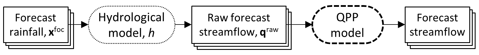
Figure 1 Illustration of general approach used to produce streamflow forecasts. Layers represent ensemble members.

The deterministic hydrological model, $h({\mathit{\theta }}_h;{\mathit{x}}_t,{\mathit{s}}_{t-\mathrm{1}})$, has a (single) set of parameters θ_h, inputs x_t (including forecast rainfall x^foc), and states s_t−1 at time t−1. In general, any rainfall–runoff model can be used for this purpose; in our case study, we employ the rainfall–runoff model GR4J (Perrin et al., 2003; see Sect. 3.2).

The streamflow forecasts are obtained in two steps. First, an ensemble of N_foc rainfall forecasts $\mathit{\{}{\mathit{x}}^{\text{foc}\left(f\right)};f=\mathrm{1},\mathrm{\dots },N_{\text{foc}}\mathit{\}}$ generated by a numerical weather prediction model are propagated through the deterministic hydrological model to generate a corresponding ensemble of raw streamflow forecasts, $\mathit{\{}{\mathit{q}}^{\text{raw}\left(f\right)};f=\mathrm{1},\mathrm{\dots },N_{\text{foc}}\mathit{\}}$. Second, a probabilistic streamflow post-processing model is applied to the raw forecasts to generate the (post-processed) streamflow forecasts $\mathit{\{}{\mathit{q}}^{\left(f\right)};f=\mathrm{1},\mathrm{\dots },N_{\text{foc}}\mathit{\}}$.

The streamflow post-processing models are constructed using the residual error modelling approach. They comprise a deterministic component and a residual error model. The residual error model employs a streamflow transformation to represent the heteroscedasticity and skew of the errors, an autoregressive term to represent error persistence, and components to capture other features of errors such as seasonality.

We consider two forecasting methods which differ in the structure and details of the streamflow post-processing model as follows, with a schematic representation of these models shown in Fig. 2a:

• Seamless MuTHRE streamflow post-processing model (McInerney et al., 2020). The residual error model is formulated at the daily scale and is applied directly to (daily) raw streamflow forecasts. Conceptually, the ensemble of raw streamflow forecasts accounts for forecast rainfall uncertainty and the residual error model accounts for hydrological uncertainty.

• Non-seamless monthly streamflow post-processing (QPP) model (Woldemeskel et al., 2018). The residual error model is formulated at the monthly scale. It is applied to raw streamflow forecasts aggregated to the monthly scale and collapsed to their median value. Conceptually, the residual error model accounts for both hydrological and forecast rainfall uncertainty.

The post-processing models also differ in their parameter estimation (calibration) procedure. Figure 2b shows that the MuTHRE model is calibrated using observed daily rainfall and observed daily streamflow, whereas the monthly QPP model is calibrated to forecast daily rainfall and observed monthly streamflow (see Sects. 2.3.4 and 2.4.4 for details).

Figure 2 Conceptual diagrams of the seamless MuTHRE model and the non-seamless monthly QPP model. Ensemble components are indicated with multiple layers. Panel (a) shows the post-processing model structure, including the deterministic component and the residual error model (REM). Panel (b) shows the calibration approach to estimate the parameters of the streamflow post-processing model. Panel (c) illustrates the key distinction between the forecasting products generated by the models, where the MuTHRE model produces seamless daily streamflow forecasts that can be used at a range of lead times and aggregation periods (e.g. daily, weekly, fortnightly, and monthly), whereas the monthly QPP model produces only monthly forecasts.

Figure 2c illustrates the key operational distinction between the models. The MuTHRE model produces seamless daily streamflow forecasts that can be used at a range of lead times and aggregation periods (e.g. daily, weekly, fortnightly, and monthly). In contrast, the monthly QPP model produces only 1-month-ahead non-seamless monthly forecasts.

The next section presents common features of the post-processing models before moving to specific model details.

2.2 Streamflow post-processing model

2.2.1 Deterministic component

The deterministic component $q_t^{\text{det}}$ is obtained from the raw streamflow forecasts (Fig. 2a). The deterministic component used in the seamless MuTHRE and non-seamless monthly streamflow post-processing approaches are detailed in Sects. 2.3.2 and 2.4.2 respectively.

2.2.2 Residual error model

The residual error model describing the relationship between the probabilistic streamflow estimate Q_t and the deterministic component $q_t^{\text{det}}$ is formulated as additive in transformed space, as follows:

$$\begin{array}{}\text{(1)}& z(Q_t;{\mathit{\theta }}_z)=z(q_t^{\text{det}};{\mathit{\theta }}_z)+{\mathit{\eta }}_t,\end{array}$$

where η_t is a random residual error term.

The transformation z, with parameters θ_z, is used to reduce the heteroscedasticity and skewness in residuals. We choose the Box–Cox transformation (e.g. Box and Cox, 1964),

$$\begin{array}{}\text{(2)}& z(q;\mathit{\lambda },A)=\left\{\begin{array}{ll}\frac{(q+A{)}^{\mathit{\lambda }}-\mathrm{1}}{\mathit{\lambda }}& \text{if }\mathit{\lambda }\ne \mathrm{0}\\ \log (q+A)& \text{otherwise},\end{array}\right.\end{array}$$

with parameters ${\mathit{\theta }}_z=\mathit{\{}\mathit{\lambda },A\mathit{\}}$. The power parameter λ is set to 0.2 in both streamflow post-processing models (McInerney et al., 2017). In the seamless MuTHRE model, the offset parameter A is inferred as part of the hydrological model calibration (McInerney et al., 2020), while in the non-seamless monthly QPP model, it is set to 1 % of the mean observed monthly streamflow, i.e. $A=\mathrm{0.01}\times \text{mean}\left({\stackrel{\mathrm{̃}}{\mathit{q}}}^{\text{mon}}\right)$ (Woldemeskel et al., 2018).

The residual error term η_t is standardised and then modelled as a first-order autoregressive (AR1) process, as follows:

$$\begin{array}{}\text{(3)}& {\displaystyle }{\mathit{\nu }}_t={\displaystyle \frac{{\mathit{\eta }}_t-{\mathit{\mu }}_t}{{\mathit{\alpha }}_t}}\text{(4)}& {\displaystyle }{\mathit{\nu }}_t={\mathit{\varphi }}_{\mathit{\eta }}{\mathit{\nu }}_{t-\mathrm{1}}+y_t,\end{array}$$

where μ_t and α_t are the (time-varying) mean and scaling factor of η_t, ϕ_η is the lag-1 autoregressive parameter, and y_t is the random component (referred to as the innovation) at time t.

When generating forecasts, recent streamflow observations are used to update errors via the AR1 model and reduce uncertainty in η_t for short lead times.

2.3 Seamless MuTHRE model

2.3.1 Model structure

The seamless MuTHRE post-processing model operates at the daily timescale. Uncertainty due to forecast rainfall and hydrological errors is represented using the ensemble dressing approach (Pagano et al., 2013). The ensemble of daily raw streamflow forecasts, q^raw, obtained by propagating an ensemble of rainfall forecasts through the hydrological model h, accounts for forecast rainfall uncertainty. A randomly generated replicate of the residual term, η, is then added to each of the N_foc raw streamflow forecast ensemble members to account for hydrological uncertainty. This produces an ensemble of N_foc post-processed streamflow forecasts (see the schematic in Fig. 2a). Note that this approach to capturing forecast rainfall and hydrological uncertainty requires the rainfall forecasts to be reliable in order to produce reliable streamflow forecasts (Verkade et al., 2017).

2.3.2 Deterministic component

In the context of Eq. (1), the deterministic component in the MuTHRE model at its daily time step t is as follows:

$$\begin{array}{}\text{(5)}& q_t^{\text{det}}=q_t^{\text{raw}\left(f\right)}=h({\mathit{\theta }}_h;{\mathit{x}}_t^{\left(f\right)},{\mathit{s}}_{t-\mathrm{1}}),\end{array}$$

i.e. the residual error model is applied directly to each ensemble member of the raw forecasts (Fig. 2a).

2.3.3 Residual error model

The MuTHRE model assumes that the mean of the residual error – μ_t in Eq. (3) – varies in time due to seasonality and dynamic biases (associated with hydrologic non-stationarity), as follows:

$$\begin{array}{}\text{(6)}& {\mathit{\mu }}_t={\mathit{\mu }}_{d\left(t\right)}^{\text{(s)}}+{\mathit{\mu }}_t^{\text{(b)}}+{\mathit{\mu }}^{\ast }.\end{array}$$

The seasonality component ${\mathit{\mu }}_{d\left(t\right)}^{\text{(s)}}$ describes the mean value of μ on the day-of-the-year d(t), the dynamic bias term ${\mathit{\mu }}_t^{\text{(b)}}$ describes the mean value of μ (after removing seasonality) over the preceding N_b d (N_b=30 is used), and μ^∗ is a constant to capture the remaining bias. Full details of these terms are provided in McInerney et al. (2020).

The scaling factor – α_t in Eq. (3) – is constant (set to 1 for simplicity).

Innovations are modelled using a two-component mixed Gaussian distribution as follows:

$$\begin{array}{}\text{(7)}& y_t\sim {\mathcal{N}}_{\text{mix}}({\mathit{\mu }}_{\mathrm{1}},{\mathit{\sigma }}_{\mathrm{1}}^{\mathrm{2}},{\mathit{\mu }}_{\mathrm{2}},{\mathit{\sigma }}_{\mathrm{2}}^{\mathrm{2}},w_{\mathrm{1}}),\end{array}$$

where μ₁ and μ₂ are the means of the two components, which are set to zero, σ₁ and σ₂ are the standard deviations of the components, and w₁ is the weight of the first component. Compared to a standard Gaussian distribution, the mixed Gaussian distribution allows for fatter tails (i.e. excess kurtosis) in the distribution of innovations, which has been shown to improve reliability of daily forecasts at short lead times (Li et al., 2016). Note that the mixed Gaussian distribution does not offer benefits at longer lead times, nor when aggregating forecasts to the monthly scale (McInerney et al., 2020).

2.3.4 Calibration of residual error model

The parameters of the residual error model $\mathit{\{}{\mathit{\mu }}^{\text{(s)}},{\mathit{\mu }}^{\text{(b)}},{\mathit{\mu }}^{\ast },{\mathit{\varphi }}_{\mathit{\eta }},{\mathit{\sigma }}_{\mathrm{1}}^{\mathrm{2}},{\mathit{\sigma }}_{\mathrm{2}}^{\mathrm{2}},w_{\mathrm{1}}\mathit{\}}$ are estimated from the following daily scale data (see Fig. 2b):

1. daily hydrological model simulations q^sim forced with observed rainfall $\stackrel{\mathrm{̃}}{\mathit{x}}$

2. daily observed streamflow $\stackrel{\mathrm{̃}}{\mathit{q}}$.

Seasonality (μ^(s)) and dynamic bias (μ^(b)) terms are calculated using moving averages, parameters μ^∗ and ϕ_η are estimated as the sample mean and lag-1 auto-correlation of the detrended residuals, while the mixed Gaussian parameters $\mathit{\{}{\mathit{\sigma }}_{\mathrm{1}}^{\mathrm{2}},{\mathit{\sigma }}_{\mathrm{2}}^{\mathrm{2}},w_{\mathrm{1}}\mathit{\}}$ are estimated using maximum likelihood. Full details of the calibration procedure are provided in McInerney et al. (2020).

2.4 Non-seamless monthly QPP model

2.4.1 Model structure

The non-seamless monthly QPP model operates at the monthly timescale. The raw forecasts are aggregated from daily to monthly scale and collapsed to their median value yielding q^det,mon, i.e. the uncertainty from the raw streamflow ensemble is discarded. The combined forecast rainfall uncertainty and hydrological uncertainty are represented through the residual error term η. Monthly streamflow forecasts are obtained from q^det,mon by adding N_foc replicates of η (see the schematic in Fig. 2a).

2.4.2 Deterministic component

The deterministic component in the non-seamless model at its monthly time step t is computed as follows:

$$\begin{array}{}\text{(8)}& {\displaystyle }{q}_t^{\text{raw,mon}\left(f\right)}=\text{average}(q_{t^{\ast }}^{\text{raw}\left(f\right)};t^{\ast }\in T(t\left)\right)\text{(9)}& {\displaystyle }{q}_t^{\text{det}}=\text{median}(q_t^{\text{raw,mon}\left(f\right)};f=\mathrm{1},\mathrm{\dots },N_{\text{foc}}),\end{array}$$

where T(t) is averaging window (range of days) corresponding to the monthly time step t.

2.4.3 Residual error model

The residual error model is applied at the monthly scale after collapsing the ensemble of raw forecasts to a single time series.

The monthly residual error model captures seasonality in residuals by varying the mean μ_t and scaling factor α_t in Eq. (3) by month. Innovations are assumed to be independent and identically distributed Gaussian, as follows:

$$\begin{array}{}\text{(10)}& y_t\sim \mathcal{N}(\mathrm{0},{\mathit{\sigma }}_y^{\mathrm{2}}),\end{array}$$

where σ_y is the standard deviation of the innovations.

2.4.4 Calibration of residual error model

The parameters of the monthly residual error model $\mathit{\{}{\mathit{\varphi }}_{\mathit{\eta }},{\mathit{\sigma }}_y^{\mathrm{2}},\mathit{\{}{\mathit{\mu }}_m,{\mathit{\alpha }}_m;m=\mathrm{1},\mathrm{\dots },\mathrm{12}\mathit{\left\}}\mathit{\right\}}$ are estimated from the following monthly scale data (see Fig. 2b):

1. monthly deterministic forecasts q^det,mon obtained using forecast rainfall (as described in Sect. 2.4.2)

2. monthly observed streamflow ${\stackrel{\mathrm{̃}}{\mathit{q}}}^{\text{mon}}$.

All parameters are calibrated using the method of moments. Full details are provided in Woldemeskel et al. (2018).

3 Case study

3.1 Catchments and data

The case study uses a set of 11 catchments from the Murray–Darling basin in Australia, including four catchments on the Upper Murray River (New South Wales and Victoria) and seven catchments on the Goulburn River (Victoria). These catchments have winter-dominated rainfall which leads to higher streamflow between June and October (see Fig. 3) and have less than 5 % of days with no flow. Catchment properties are summarised in Table 1. This same set of catchments was used to extensively evaluate the MuTHRE model in McInerney et al. (2020).

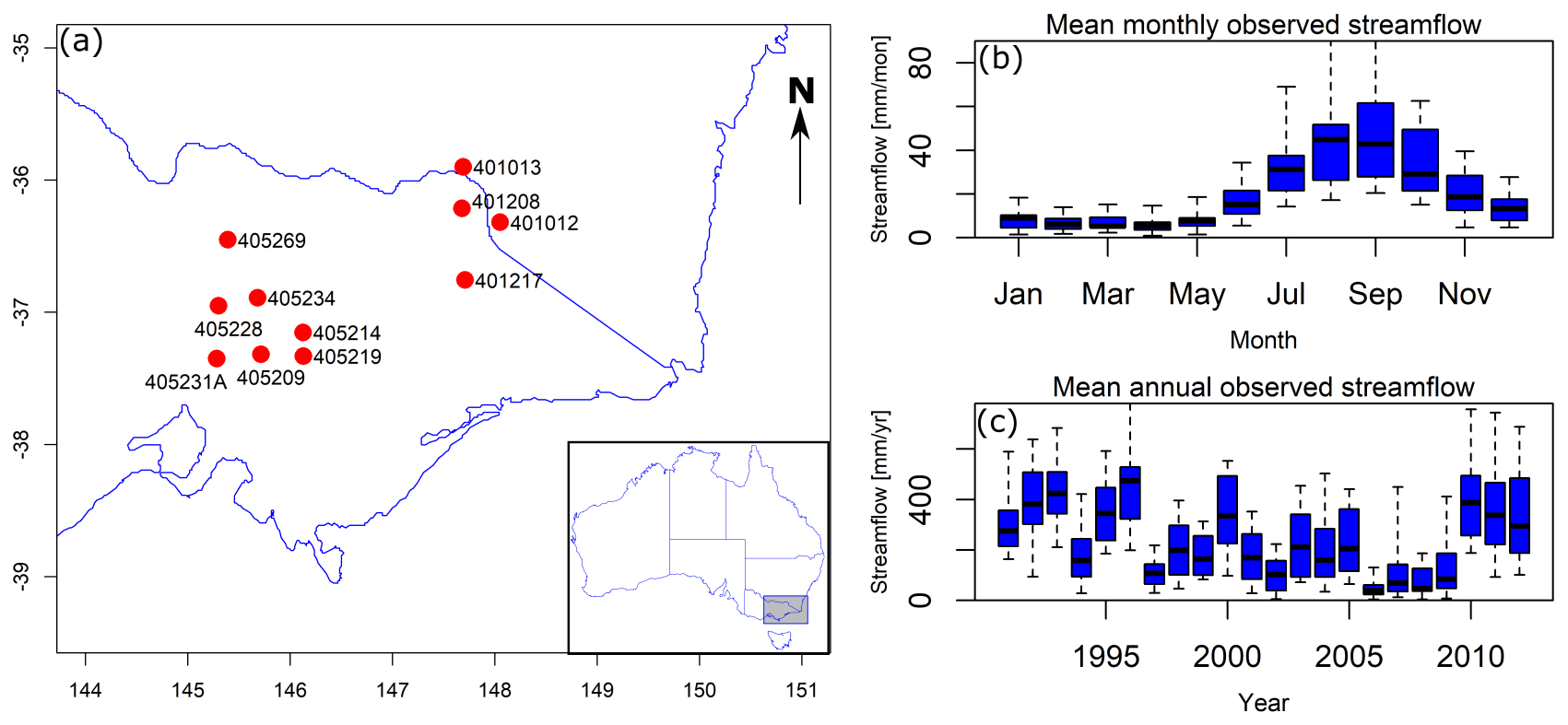
Figure 3 Location of the 11 case study catchments (a) and mean observed streamflow for each month (b) and each year (c). Box plots in panels (b) and (c) show distributions of mean observed streamflow over the 11 catchments.

Table 1 Properties of the 11 case study catchments.

Time series of daily observed streamflow over a 22-year period between 1991 and 2012 are obtained from the Hydrologic Reference Stations (HRS) dataset (http://www.bom.gov.au/water/hrs, last access: 8 November 2022). Observed rainfall and potential evapotranspiration (PET) data over the same period are obtained from the Australia Bureau of Meteorology's climate data service (http://www.bom.gov.au/climate, last access: 8 November 2022), with a climatological average used for PET (McInerney et al., 2021a).

Rainfall forecasts are provided by the Australian Community Climate and Earth System Simulator – Seasonal (ACCESS-S; Hudson et al., 2017). The ACCESS-S rainfall forecasts are pre-processed using the method of Schepen et al. (2018) in order to reduce biases and improve the reliability in comparison to observed rainfall. An ensemble of 100 pre-processed rainfall forecasts that begin on the first day of each month and extend out to a maximum lead time of 1 month are used.

3.2 Hydrological model

The conceptual rainfall–runoff model GR4J (Perrin et al., 2003) is used as the deterministic hydrological model h for simulating daily streamflow from rainfall and PET inputs (see Sect. 2.1). GR4J has been widely used and evaluated over diverse catchment climatologies and physical characteristics (Perrin et al., 2003; Hunter et al., 2021). GR4J represents the processes of interception, infiltration, and percolation and has four calibration parameters, where x₁ is the capacity of the production store (mm), x₂ is the water exchange coefficient (mm), x₃ is the capacity of the routing store (mm), and x₄ is the time parameter of the unit hydrograph (d).

3.3 Calibration/evaluation procedure

Calibration of model parameters and evaluation of forecasts is performed using a leave-1-year-out cross validation procedure (McInerney et al., 2020). For each calendar year j, hydrological and residual error model parameters are calibrated using observed streamflow data from the entire evaluation period, except for year j and the subsequent years j+1 to j+4 (which are excluded to reduce the influence of system memory on model evaluation, as described in Pokhrel et al., 2013). Hydrological model parameters are estimated using likelihood maximisation based on the BC0.2 error model (McInerney et al., 2020), implemented using a quasi-Newton optimisation algorithm run with 100 independent multistarts (Kavetski and Clark, 2010). Methods for estimating residual error model parameters are described in Sects. 2.3.4 and 2.4.4.

Note that, in this work, we do not consider parametric uncertainty (in the hydrological and residual error models), which is expected to be a (relatively) minor contributor to total forecast uncertainty, given the long data period used in the estimation; this simplification is common in contemporary forecasting implementations (e.g. Engeland and Steinsland, 2014; Verkade et al., 2017).

For each year j, calibrated hydrological and error models are used to generate an ensemble of 100 streamflow forecasts. Daily forecasts from the MuTHRE model begin on the first day of each month and extend out to a maximum lead time of 1 month (which is the same as the rainfall forecasts).

This calibration/forecasting process is repeated for all 22 years, resulting in 22 sets of 1-year forecasts, which are subsequently merged into a single 22-year forecast to facilitate evaluation against streamflow observations.

3.4 Forecast evaluation

3.4.1 Performance metrics

Streamflow forecasts are evaluated using numerical metrics for the following attributes:

• Reliability refers to the degree of statistical consistency between the forecast distribution and the observed data. It is evaluated using the reliability metric of Evin et al. (2014). Lower metric values are better, with 0 representing perfect reliability and 1 representing the worst reliability.

• Sharpness refers to the spread of the forecast distribution, with sharper forecasts being those with lower spread. We use the sharpness metric of McInerney et al. (2020), which is based on the ratio of the average 90 % interquantile range (IQR) of the forecasts and a climatological distribution (described below). Lower values are better, with 0 representing a deterministic forecast (with no spread) and 1 representing the same sharpness as climatology. In contrast to the other attributes considered here, sharpness is a property of the forecast only and does not depend on the observed data.

• Volumetric bias refers to the long-term water balance error. It is quantified using the metric of McInerney et al. (2017) as the relative absolute difference between total observed streamflow and the total forecast streamflow (averaged over the forecast ensemble). Lower values are better, with 0 representing unbiased forecasts.

• Combined performance is quantified using the continuous ranked probability score (CRPS). The CRPS is defined as the sum of squared differences between forecast cumulative distribution function (CDF) and the empirical CDF of the observation. Note that the CRPS can be decomposed into terms representing individual performance aspects, namely reliability, and uncertainty/resolution (related to sharpness; Hersbach, 2000). We express this metric as a skill score (CRPSS) relative to the climatological distribution. Higher CRPSS values are better, with a value of 1 representing a perfectly accurate deterministic forecast and 0 representing the same skill as the climatological distribution.

The climatological distribution represents the distribution of daily streamflow for a given time of the year based solely on previously observed streamflow at that time of the year. It is constructed using a 29 d moving window approach, which is described in detail in McInerney et al. (2020).

3.4.2 Aggregation and stratification

The study focuses on the performance of the streamflow post-processing models at the monthly scale. The monthly MuTHRE forecasts are obtained by aggregating daily forecasts to the monthly scale. The monthly QPP model generates monthly forecasts directly.

Overall evaluation of monthly forecasts is performed using data from the entire evaluation period, i.e. all months and years, with more detailed stratified performance evaluation performed for individual months and years.

We also demonstrate the ability of the MuTHRE model to produce seamless forecasts, which are reliable over a range of lead times and aggregation scales. This is achieved by evaluating both (i) daily forecasts stratified by lead times from 1 to 28 d and (ii) cumulative flow forecasts for periods of 1–28 d. The forecast is considered to be seamless if reliability metrics are similar across all lead times and aggregation scales. The evaluation of cumulative flow forecasts expands on the analysis of McInerney et al. (2020), who evaluated only daily and monthly forecasts, and provides and important demonstration of seamless forecasting over the entire range of timescales from 1 to 28 d. We note that cumulative flow forecasts over 1 month correspond to monthly forecasts.

3.4.3 Evaluation of practical significance of differences between streamflow post-processing models

Forecast performance of the two streamflow post-processing models is compared across multiple catchments using practical significance tests, as described next. For each combination of performance metric (e.g. reliability) and stratification (e.g. month), a statistical test is used to determine whether differences in metric values over the range of catchments exceed a predefined margin representing practical significance (relevance).

The statistical tests are performed using the paired Wilcoxon signed rank test (Bauer, 1972), with controls applied to reduce the false discovery rate to 5 %, corresponding to a confidence level of 95 % (Wilks, 2006; Benjamini and Hochberg, 1995). The practical significance margin is taken as 20 % of the median metric value for the non-seamless monthly QPP model (following McInerney et al., 2020).

4 Results

4.1 Demonstration of seamless forecasting capabilities of the MuTHRE model

4.1.1 Daily forecasts

Figure 4 illustrates the streamflow forecast time series in the Biggara catchment (catchment ID 401012; see Fig. 3). Daily forecasts from the seamless MuTHRE model for a representative time period beginning on 1 May 2002 are shown in Fig. 4a. The observed daily streamflow lies within the 90 % probability limits of the MuTHRE forecasts for each lead time. As expected, the probability limits are tight for short lead times (when forecast rainfall uncertainty and hydrological uncertainty are small) and widen for longer lead times.

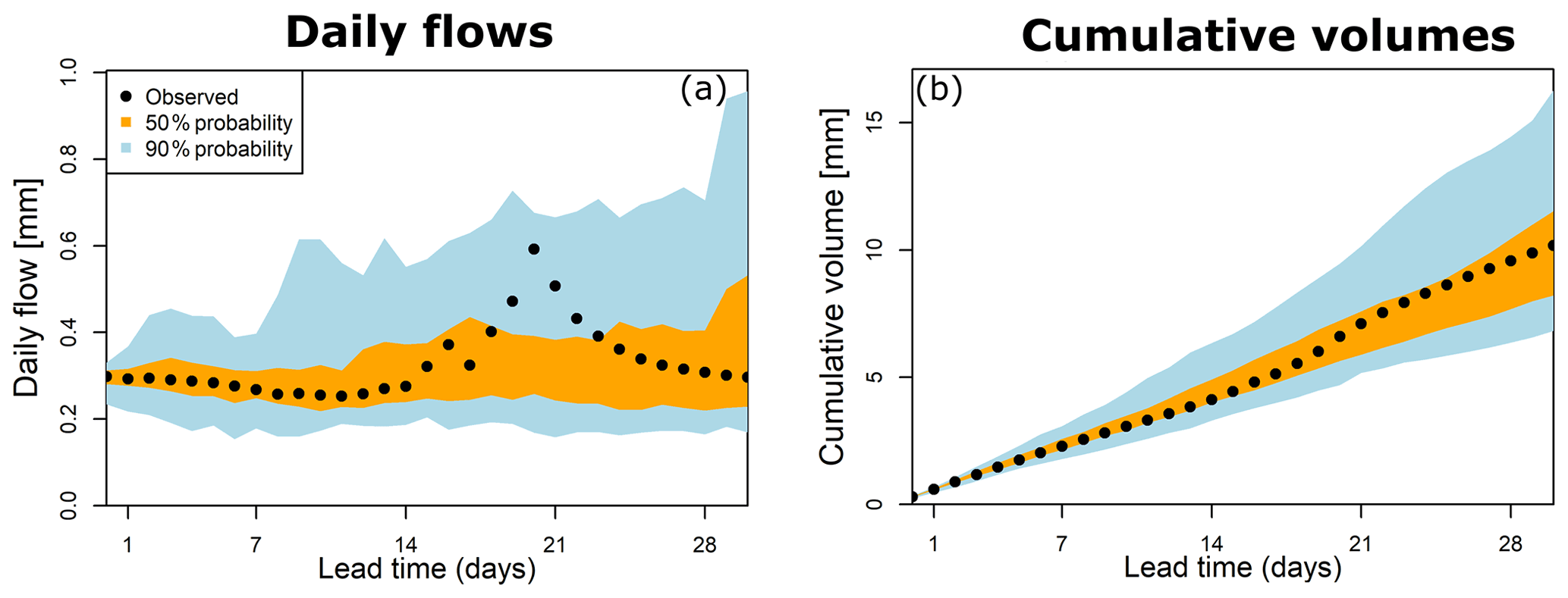
Figure 4 Time series of daily and cumulative probabilistic forecasts from the seamless MuTHRE model for the Murray River at Biggara (401012; see Fig. 3) for May 2002. The non-seamless monthly QPP model does not have the capability to produce these forecasts.

Figure 5 (left column) shows the performance of daily forecasts from the MuTHRE model for lead times of 1 to 28 d, evaluated over all case study catchments. The key finding from this analysis is that reliability is relatively constant over all lead times, with median metric values lying in the tight range of 0.04–0.06 (Fig. 5a). We also note that forecasts are sharper and have better CRPSS at short lead times and that bias is relatively constant.

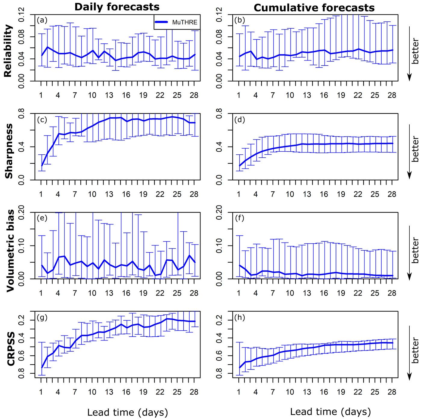
Figure 5 Performance of MuTHRE forecasts in terms of daily streamflow (a, c, e, g) and cumulative flow (b, d, f, h). Metrics are shown for reliability (a, b), sharpness (c, d), volumetric bias (e, f), and CRPSS (g, h). The bars indicate the full range of metric values across the 11 case study catchments, and the line indicates the median metric values. Note the inverted y axis, for CRPSS, for visual consistency with the other metrics.

4.1.2 Cumulative flow forecasts

Figure 4b shows cumulative flow forecasts out to 28 d in the Biggara catchment for the representative time period. The cumulative flows based on observed streamflow lie well within the 90 % probability limits of the MuTHRE forecasts for all lead times.

Figure 5 (right column) shows the performance of cumulative flow forecasts from the MuTHRE model for lead times of 1 to 28 d over all catchments. Again, we see that reliability is relatively constant over all lead times, with median metric values between 0.04 and 0.06 (Fig. 5b). We also note that sharpness, volumetric bias, and CRPSS metrics are typically better for cumulative forecasts than for daily forecasts (compare the left and right columns in Fig. 5).

In summary, the forecasts from the MuTHRE model are seamless because they are reliable over (a) the range of lead times and (b) multiple aggregation scales, from the shortest scale of 1 d to the longest scale of 1 month, and everything in between. This result confirms and extends previous findings in McInerney et al. (2020), who focused on daily and monthly scales only. In contrast to the seamless MuTHRE model, the non-seamless monthly QPP model does not have the capability to produce forecasts of daily streamflow and cumulative flows for time periods below 1 month.

4.2 Comparison of monthly forecasts

Figure 6 compares monthly forecasts from the seamless MuTHRE model and non-seamless monthly QPP model for the Biggara catchment. While there are some minor differences between the two forecasts (e.g. the monthly QPP model produces larger spread than the MuTHRE model during 2010), the two forecasts are clearly very similar.

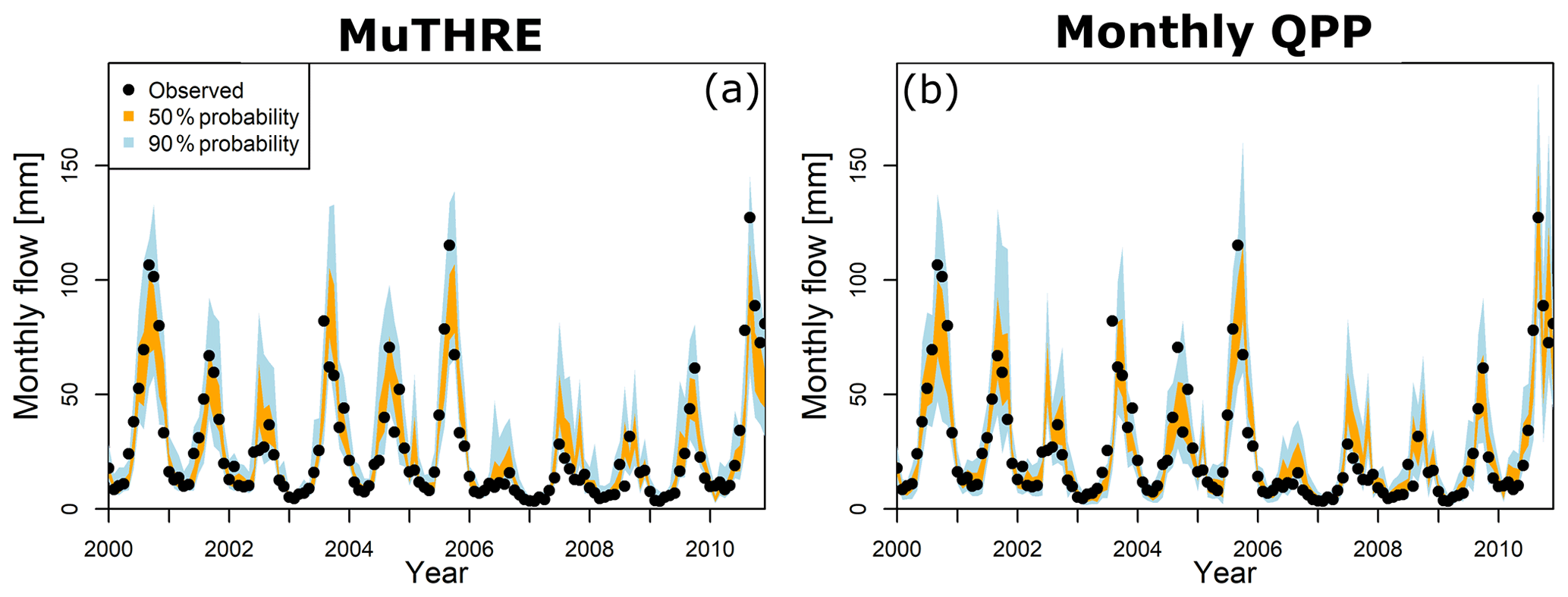
Figure 6 Time series of monthly probabilistic forecasts for Murray River at Biggara (401012; see Fig. 3), for the seamless MuTHRE model and non-seamless monthly QPP model. Results are shown between the years 2000 and 2011.

Figure 7 compares monthly forecasts from the MuTHRE and monthly QPP models in terms of overall performance (left column) and when stratified by month (middle column) and year (right column). The key findings are as follows.

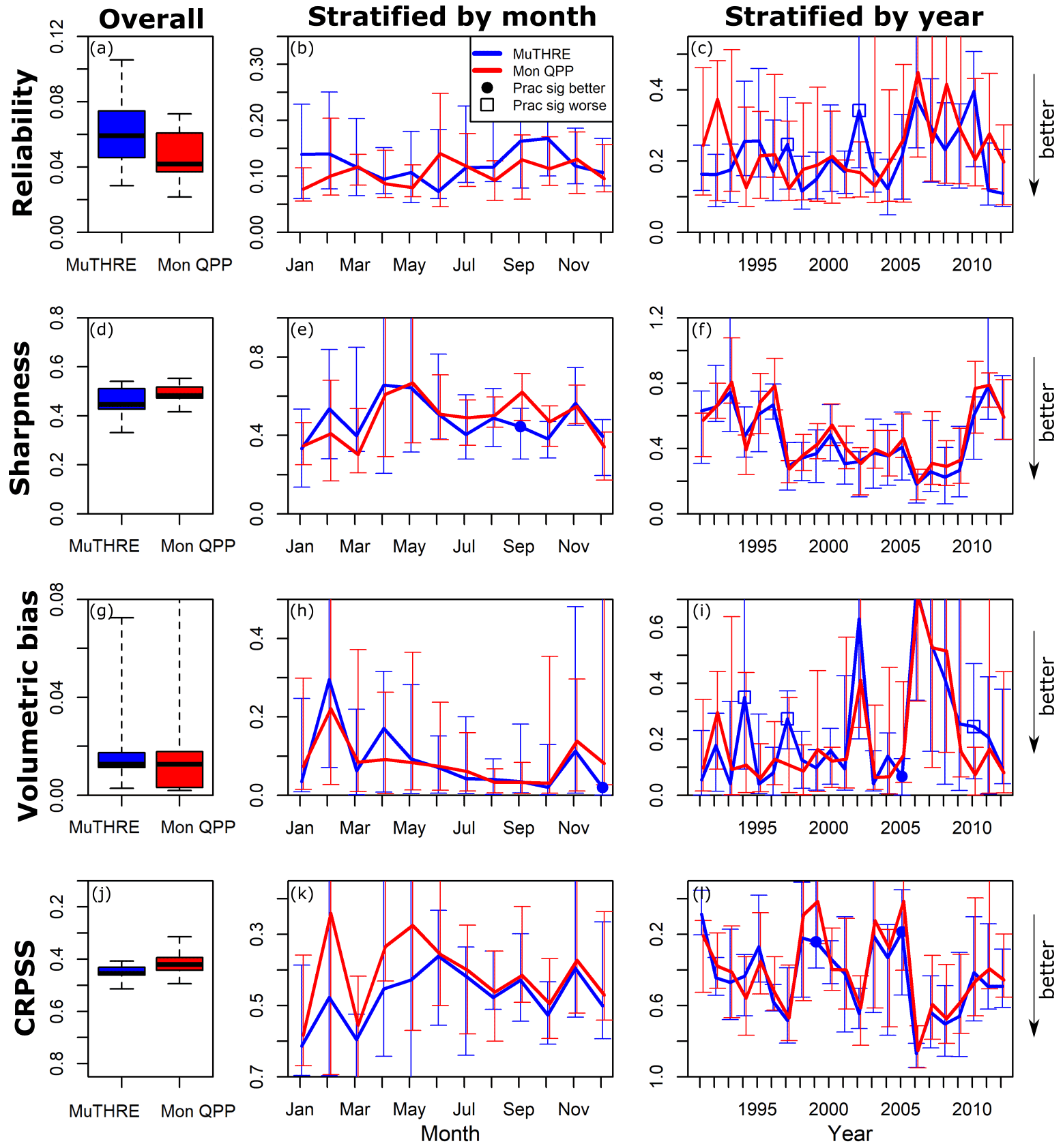
Figure 7 Overall performance (all months and years; a, d, g, j), performance stratified by month (b, e, h, k), and performance stratified by year (c, f, i, l) of monthly forecasts from the seamless MuTHRE and non-seamless monthly QPP models. Results are shown for reliability (a–c), sharpness (d–f), volumetric bias (g–i), and CRPSS (j–l). Box plots in the left column (a, d, g, j) show the distribution of metric values over the 11 catchments. In the other columns (b, c, e, f, h, i, k, l), vertical bars indicate the full range of metric values across the catchments, the line indicates the median metric values, and circles/squares indicate that the MuTHRE model performs practically significantly better/worse than the monthly QPP model.

Reliability. Figure 7a shows similar overall reliability of monthly forecasts from the MuTHRE and monthly QPP models. While the median metric value of 0.06 for the MuTHRE model is worse than the median value of 0.04 for the monthly QPP model, these differences are not practically significant (based on the test described in Sect. 3.4.3). Figure 7b shows that, when performance is stratified by month, the two models have similar reliability (i.e. not practically significant) for all 12 months. When stratified by year, the MuTHRE model achieves similar reliability to the monthly QPP model for 20 out of the 22 years, while the monthly QPP model achieves practically significant improvements in 2 of the 22 years (Fig. 7c).

Sharpness. Figure 7d shows that the overall sharpness of monthly forecasts from the MuTHRE model is slightly better than the monthly QPP model (median metric values of 0.44 compared with 0.49), although differences are not practically significant. Figure 7e shows that, when sharpness is stratified by month, the MuTHRE model provides practically significant improvement in September and similar performance in the other 11 months. Figure 7f shows that the sharpness stratified by year is similar for both models for all years.

Volumetric bias. Figure 7g shows that the overall volumetric bias from both models is similar (median of 0.01). Figure 7h shows that, when stratified by month, the MuTHRE model produces practically significant improvements in December and similar performance in the remaining 11 months. Figure 7i shows that, when stratified by year, the MuTHRE model produces practically significant improvements in 1 year (2005), and the monthly QPP model provides practically significant improvements in 3 years, with similar performance in the remaining 18 years.

CRPSS. In terms of overall CRPSS, Fig. 7j shows that the MuTHRE model (median metric value of 0.45) provides slight improvement over the monthly QPP model (median metric value of 0.42), although these differences are not practically significant. Figure 7k shows that, when stratified by month, the MuTHRE model provides similar performance in all 12 months. Figure 7i shows that, when performance is stratified by year, the MuTHRE model provides practically significant improvements in CRPSS in 2 out of 22 years, with a similar performance in the remaining 20 years.

In summary, aggregated forecasts from the seamless MuTHRE model offer similar (not practically significant) and, in some cases, superior performance to forecasts from the non-seamless monthly QPP model, for the vast majority of performance metrics and stratifications considered in this study.

5 Discussion

5.1 Interpretation of key findings

The empirical results show that the seamless MuTHRE model achieves essentially the same performance as the non-seamless monthly QPP model at the monthly timescale and even provides improvement in some aspects. At first glance, this outcome may seem surprising for the following reasons:

• The seamless MuTHRE model is required to produce reliable forecasts over a range of lead times and aggregations scales, whereas the non-seamless monthly QPP model is only required to produce reliable monthly streamflow forecasts.

• The seamless MuTHRE model is calibrated at the daily scale, using only observed daily streamflow during calibration, while the non-seamless monthly QPP model is calibrated to match the observed monthly streamflow.

• The seamless MuTHRE model does not see the forecast rainfall during calibration, whereas the non-seamless monthly QPP model does.

The subsections below describe how the seamless MuTHRE model is able to achieve comparable/better performance than the non-seamless monthly QPP model despite these apparent challenges.

5.1.1 Timescale of forecasting/calibration

The seamless MuTHRE model produces daily forecasts that can be aggregated from timescales of 1 d to 1 month, whereas the non-seamless monthly QPP model produces forecasts only at the monthly scale. One might expect the enhanced capability obtained from the seamless MuTHRE model to come at some cost in performance at the monthly scale. Encouragingly, this is not the case.

The ability to reliably aggregate daily forecasts to the monthly scale demonstrates that the seamless MuTHRE model is adequately capturing temporal persistence in daily forecasts. The MuTHRE model represents temporal persistence in hydrological errors using the daily Eq. (1) model and the (30 d) dynamic bias component. This is important because neglecting temporal persistence in hydrological errors can result in an underestimation of hydrological uncertainty for aggregated predictions/forecasts (Evin et al., 2014). The reliability of aggregated forecasts also suggests that the (pre-processed) rainfall forecasts are capturing the day-to-day temporal persistence of the observed rainfall required to produce reliable monthly rainfall forecasts (see Sect. 5.1.2).

The seamless MuTHRE model is not calibrated to optimise performance at the monthly scale, as it uses only observed daily streamflow during calibration. On the other hand, the non-seamless monthly QPP model is calibrated to match the observed monthly streamflow, which could lead to improved performance at the monthly scale compared to the seamless MuTHRE model. As such, the comparable performance of the MuTHRE model at the monthly scale is particularly encouraging given that monthly data are not used in its calibration.

5.1.2 Use of observed vs. forecast rainfall used in calibration

Both approaches use the same deterministic hydrological model calibrated using observed rainfall and streamflow data. However, due to structural differences in their representation of residual errors, the seamless MuTHRE and non-seamless monthly QPP models differ in the approach used to calibrate the residual error model parameters. The residual error model in the non-seamless monthly QPP model represents combined rainfall and hydrological uncertainty. It uses forecast rainfall during calibration and can (in theory) correct for biases and under-/overdispersion in rainfall forecasts. In contrast, the seamless MuTHRE model represents only hydrological uncertainty and is calibrated using observed rainfall. Uncertainty due to forecast rainfall is represented by propagating rainfall forecasts through the hydrological model. Since the MuTHRE model does not correct for forecast rainfall errors, this approach requires rainfall forecasts to be reliable in order to produce reliable streamflow forecasts (Verkade et al., 2017).

In this study we have used rainfall forecasts from the ACCESS-S numerical weather prediction model (Hudson et al., 2017), which were pre-processed at the catchment scale with the aim of reducing biases and over-/underdispersion at the daily scale and capturing the temporal persistence in rainfall (Schepen et al., 2018). As a result, these pre-processed rainfall forecasts are reliable and sharp at both the daily and monthly scale and do not have a detrimental impact on the performance of the seamless MuTHRE model.

Since the seamless MuTHRE model uses only observed rainfall in calibration, it does not require recalibration if an improved rainfall forecast product becomes available, which is a useful advantage in operational settings. In contrast, the monthly QPP model is calibrated using forecast rainfall and must be recalibrated whenever a new rainfall forecast is to be used. Note that this is a benefit of the ensemble dressing approach used in the MuTHRE model, rather than of the forecasts being seamless.

5.1.3 Use of daily vs. monthly streamflow observations to update forecasts

The MuTHRE and monthly QPP models differ in their use of recently observed streamflow data. The MuTHRE model uses daily streamflow observations to update both (i) the dynamic bias component of the error model, to account for monthly errors, and (ii) the daily AR1 model to account for recent daily errors and improve sharpness of forecasts for short lead times. In contrast, the monthly model only uses monthly aggregated streamflow observations to update the monthly AR1 model. The ability to utilise the most recent time series of daily streamflow observations provides the MuTHRE model with a potential advantage over the monthly QPP model (which see only monthly totals) and may be another reason why the MuTHRE model performs so well compared with the monthly QPP model.

5.2 Summary of practical benefits of seamless MuTHRE forecasts

The key practical benefits that the seamless MuTHRE model provide over the non-seamless monthly QPP model are summarised below:

1. Seamless forecasts can be used to inform decisions at a range of timescales.

2. Seamless daily forecasts are easily integrated into river system models used for real-time decision-making.

3. The forecasting system is simplified as a single seamless product can serve a range of forecast requirements at different timescales.

4. Improvements in rainfall forecasting are easily integrated into the forecasting system (as described in Sect. 5.1.2).

The competitive performance of the seamless MuTHRE model, even at the native scale of the non-seamless monthly QPP forecasts, is clearly encouraging – it indicates that seamless forecasts do not require a compromise between capability (range of available forecast timescales) and performance. Proverbially speaking, a user of seamless forecasts can “have their cake and eat it too”. This finding provides further motivation to adopt seamless forecasts in research and practical work.

5.3 Future work

Future work is recommended on the following aspects:

• Further testing and development of the MuTHRE model on a wide range of catchments. The monthly QPP model has been comprehensively evaluated on 300 catchments around Australia (Woldemeskel et al., 2018), whereas the MuTHRE model has currently been evaluated on 11 catchments in the Murray–Darling basin. Evaluation of the MuTHRE model over a wide range of hydroclimatic conditions is required to ensure the findings of this study are robust. Potential enhancements of the MuTHRE model, including specialised treatment of zero flows in ephemeral catchments (McInerney et al., 2019; Wang et al., 2020), may be required to ensure the MuTHRE model remains competitive with the monthly QPP model over a wider range of flow regimes.

• Deeper understanding of the reasons for the MuTHRE model matching the monthly QPP model at the monthly scale. For example, systematic testing of different combinations of MuTHRE and monthly QPP model components could help diagnose the specific reasons why the MuTHRE model performs so well.

• Evaluation of how the quality of rainfall forecasts impacts on the performance of the seamless MuTHRE model. This includes impacts on its ability to match/improve on the performance of the non-seamless monthly QPP model at the monthly scale.

6 Conclusions

Subseasonal streamflow forecasts at timescales ranging from daily to monthly are of major interest in water management. This study compares two streamflow post-processing (QPP) models, namely the seamless daily Multi-Temporal Hydrological Residual Error (MuTHRE) model and the more traditional non-seamless monthly QPP model used in the Australian Bureau of Meteorology's dynamic forecasting system. The MuTHRE model is designed at the daily scale and can be aggregated up to the monthly scale, whereas the monthly QPP model is designed directly at the monthly scale and does not produce forecasts at the daily scale. A case study with 11 catchments in southeastern Australia, the GR4J conceptual rainfall–runoff model, and pre-processed ACCESS-S rainfall forecasts are reported.

The key finding is that the seamless MuTHRE model achieves essentially the same monthly scale performance as the non-seamless monthly QPP model for the majority of metrics (reliability, sharpness, bias, and CRPSS) and stratifications (monthly and yearly). Remarkably, the seamless post-processing model achieves high-quality forecasts (based on the metrics considered in this study) at its native daily scale and matches the performance of the non-seamless monthly model at the monthly scale, despite not being calibrated at that timescale.

Seamless subseasonal forecasts, which are reliable over a wide range of lead times (1–30 d) and timescales (daily–monthly), offer numerous practical benefits over non-seamless forecasts. For users, seamless subseasonal forecasts can inform a wide range of management decisions, from flood warning to water supply operation, while for service providers, seamless forecasts will reduce the number of forecast products that require development and operation. As such it represents a single modelling tool with great versatility. The encouraging results from this study help motivate broader adoption of seamless forecasts, as they offer additional capability without a loss in performance.