Effects of passive-storage conceptualization on modeling hydrological function and isotope dynamics in the flow system of a cockpit karst landscape

Conceptualizing passive storage in coupled flow–isotope models can improve the simulation of mixing and attenuation effects on tracer transport in many natural systems, such as catchments or rivers. However, the effectiveness of incorporating different conceptualizations of passive storage in models of complex karst flow systems remains poorly understood. In this study, we developed a coupled flow–isotope model that conceptualizes both “fast-flow” and “slow-flow” processes in heterogeneous aquifers as well as hydrological connections between steep hillslopes and low-lying depression units in cockpit karst landscapes. The model tested contrasting configurations of passive storage in the fast- and slow-flow systems and was optimized using a multi-objective optimization algorithm based on detailed observational data of discharge and isotope dynamics in the Chenqi Catchment in southwestern China. Results show that one to three passive-storage zones distributed in hillslope fast-/slow-flow reservoirs and/or depression slow-flow reservoirs provided optimal model structures in the study catchment. This optimization can effectively improve the simulation accuracy for outlet discharge and isotope signatures. Additionally, the optimal tracer-aided model reflects dominant flow paths and connections of the hillslope and depression units, yielding reasonable source area apportionment for dominant hydrological components (e.g., more than ∼ 80 % of fast flow in the total discharge) and solute transport in the steep hillslope unit of karst flow systems. Our coupled flow–isotope model for karst systems provides a novel, flexible tool for more realistic catchment conceptualizations that can easily be transferred to other cockpit karst catchments.

1 Introduction

Karst areas cover extensive areas of the Earth's surface and provide important water resources. For example, the karst region in southwestern China is one of the world's largest continuous karst areas, covering ∼ 540 × 10³ km² over eight provinces and providing water resources for more than 100 million people (Chen et al., 2018). The strong dissolution of carbonate rocks in the humid tropics and subtropics of southwestern China creates unique cockpit karst landscapes, covering an area of ∼ 140× 10³–160 × 10³ km². Such cockpit karst morphology also occurs in areas in Southeast Asia, Central America and the Caribbean. In polje/tower karst systems, depression areas are interconnected with isolated towers scattered throughout the terrain (Lyew et al., 2007). As hillslope runoff is regarded as a “water tower”, often supplying agriculture in the depression, the development of hydrological models representing the hillslope and depression hydrological functionality is a necessary prerequisite for water resource management in cockpit karst landscapes.

A wide range of hydrological models have been developed for karst areas, ranging from lumped models at the catchment scale to (semi-)distributed models with hydrological function parameterized for grid scales or landscape unit scales (Martínez-Santos and Andreu, 2010; Hartmann et al., 2013; Husic et al., 2019; Dubois et al., 2020; Ollivier et al., 2020; Xu et al., 2020; Jeannin et al., 2021; Wunsch et al., 2022). A key function of karst hydrological models is to capture the dual- or multi-phase flows in a complex porous medium, thereby capturing low velocities in the matrix and small fractures as well as very high velocities in large fractures and conduits (White, 2007; Worthington, 2009; Jourde et al., 2018; Ding et al., 2020). Model structures endowed with process-based conceptualization of complex distributed flow systems often lead to overparameterization and large uncertainties in the resulting simulations (Perrin et al., 2001; Beven, 2006; Adinehvand et al., 2017). More generally, in recent years, isotope-aided hydrological models have been developed to fully couple hydrological processes with stable isotope dynamics (Birkel and Soulsby, 2015). These coupled models are effective in quantifying hydrological functions, such as water storage, flux and ages (Long and Putnam, 2004; Carey and Quinton, 2004; Delavau et al., 2017; Chacha et al., 2018; Z. Zhang et al., 2020; Elghawi et al., 2021; Mayer-Anhalt et al., 2022), which are useful metrics to characterize the karst critical zone and associated flow systems.

In isotope-aided hydrological models, flow routing is driven by pressure gradients, creating a dynamic (active) water storage that is influenced by water balance considerations (Fenicia et al., 2010; Soulsby et al., 2011), while tracer mixing, attenuation and transport require additional storage volumes (passive storage), such as unsaturated storage below field capacity (Birkel et al., 2011b) or saturated storage at depths far below the stream or water table. The conceptual combination of active storage with passive storage in isotope-aided hydrological models enhances solute mixing and resultant tracer retardation. As summarized in Table 1, previous tracer-aided hydrological models incorporate at least one passive storage. Generally, the number of passive storages increases with the subdivision of storage according to landscape units. For example, simple models with one (unsaturated/saturated or total) storage unit have one passive-storage parameter (Barnes and Bonell, 1996; Fenicia et al., 2010; Ala-aho et al., 2017). For more complex models with at least two geographical units of uplands and lowlands, the number of passive storages could increase to between two and five (Birkel et al., 2011a; Capell et al., 2012; Birkel et al., 2015; Mayer-Anhalt et al., 2022). Although these studies have provided a useful proof of concept, assessment of alternative configurations of passive-storage functions has rarely been systematically tested.

For the complex flow systems in cockpit karst landscapes, a few studies have recently incorporated passive storage into coupled flow–isotope models for simulating hydrological and solute transport processes. For example, Zhang et al. (2019) developed a semi-distributed conceptual model for capturing discharge and isotope dynamics in the Chenqi Catchment. The model has a function for passive storage to affect isotope mixing only within a conceptual hillslope unit, but it does not incorporate any passive storages in fast and slow reservoirs in the depression unit. Chang et al. (2020) compared lumped model structures with different connections of epikarst and the underlying slow and fast reservoirs according to observations of spring discharge and electrical conductivity (EC) in the Yaji Catchment in southwestern China. They set a passive storage for the fast-flow reservoir but neglected passive storage in the slow-flow system. These previous model structures with only one passive storage (Zhang et al., 2019; Chang et al., 2020) may not always be sufficient to simulate the distributed functioning of chemical mixing between active and passive storages and the hillslope flow–depression flow interconnections. Moreover, previous coupled models (listed in Table 1) are mostly calibrated and validated only against daily and/or weekly streamflow and isotope signatures. In karst catchments, as discharge responses and isotope concentrations can vary extremely rapidly, the coarse-resolution field data cannot capture the hydrological and isotopic dynamics.

The overall aim of this study is to evaluate the effectiveness of alternative ways of incorporating passive storage into a generic coupled flow–isotope model for cockpit karst landscapes. The specific objectives were to (1) develop a model that characterizes the functions of fast- and slow-flow paths from hillslope to depression units for water and tracer transport in cockpit karst landscapes; (2) systematically test alternative passive-storage configurations into the generalized model structure using a multi-objective optimization algorithm based on detailed observational data of discharge and isotope dynamics in the Chenqi Catchment in southwestern China; and (3) identify the most appropriate model structures that most efficiently describe the hydrological functioning of the catchment in terms of simulating the streamflow and tracer responses.

Table 1 Summary of the previous studies that account for passive storages in hydrological models using at least one isotopic tracer.

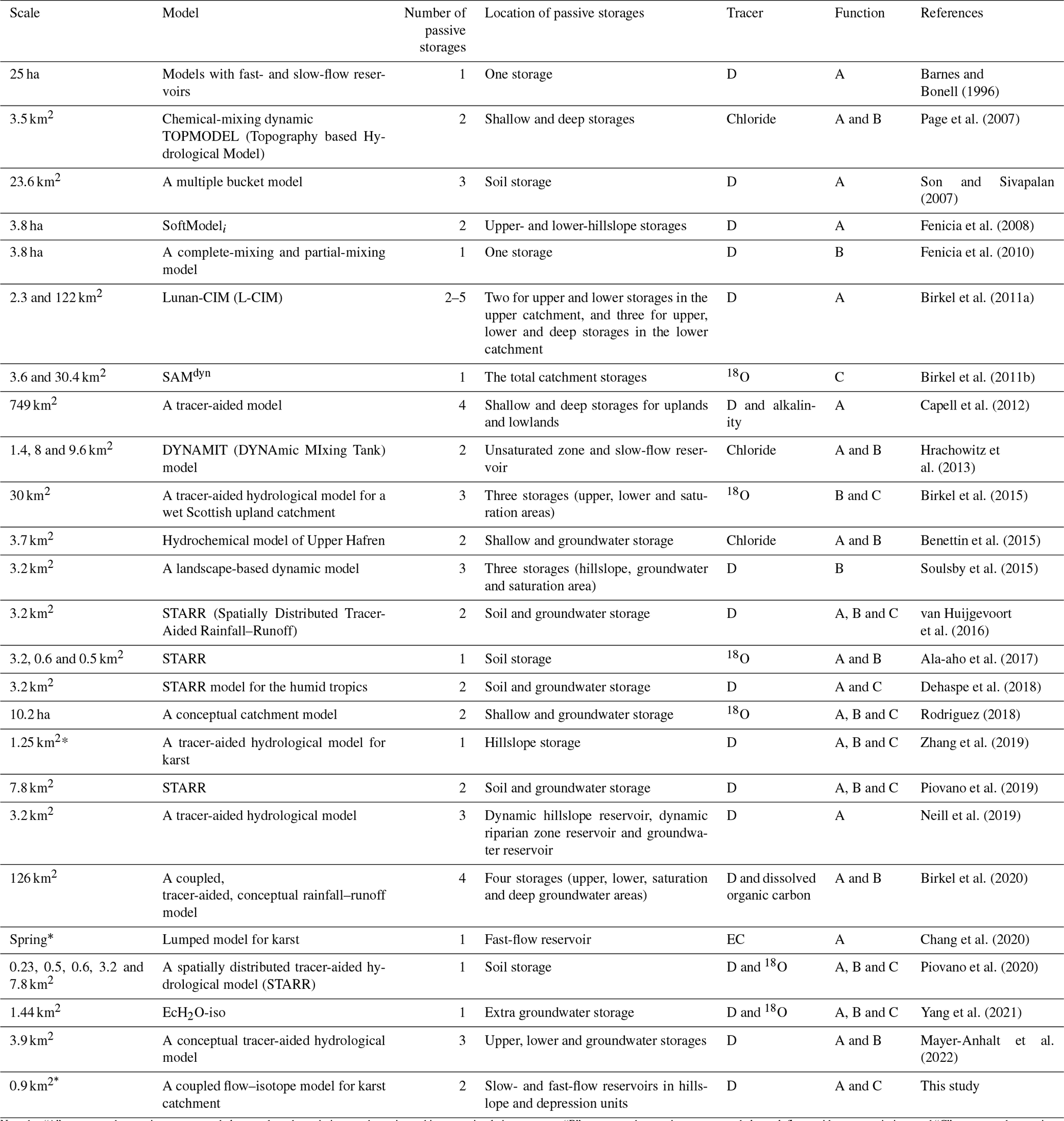
Note that “A” represents that passive storage can help reproduce the main isotope dynamics and improve simulation accuracy; “B” represents that passive storage can help track flux, resident or transit time; and “C” represents that passive storage can help estimate catchment storage. “D” is the abbreviation for deuterium. “^*” refers to application in a karst catchment.

2 Study area and data descriptions

2.1 Study area

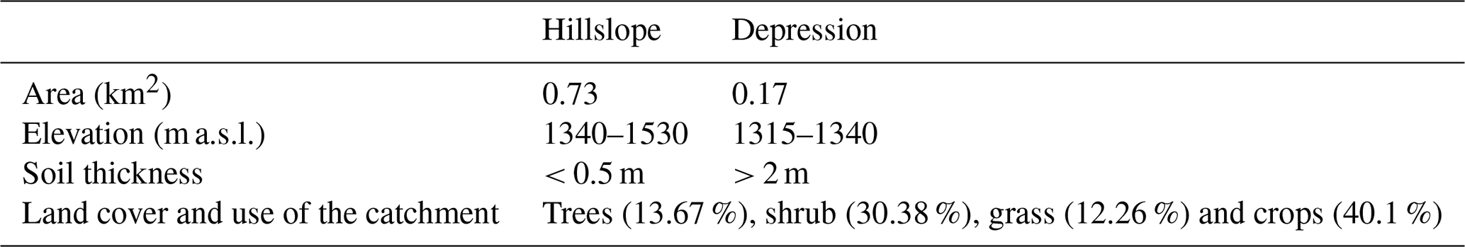
Chenqi is a small karst catchment located at the Puding Karst Ecohydrological Observation Station, Guizhou Province, southwestern China (Fig. 1). Chenqi is situated in the subtropical monsoon climate zone and experiences a mean annual temperature of 14.2 ^∘C, a mean annual rainfall of 1140 mm and a mean annual humidity of 78 %. Precipitation mainly occurs in the rainy season (May–August), accounting for more than 80 % of the annual amount. The catchment is a typical karst peak cluster landform, in which a central depression is surrounded by hillslopes with elevations ranging from 1340 to 1530 m. Considering its distinct topographic features, the catchment is conveniently divided into two dominant geomorphic units: hillslopes and depressions. These two units comprise an area of 0.73 and 0.17 km², respectively (Table 2). Due to the peak cluster depression landforms, runoff generated from hillslopes mostly flows into depression aquifers prior to contributing to streamflow at the catchment outlet (Zhang et al., 2019; R. Zhang et al., 2020).

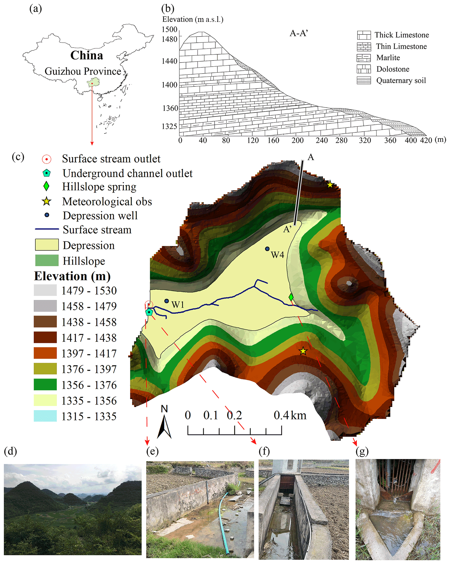
Figure 1 The location of Chenqi Catchment (a); the stratigraphic profile (b) and topography of the catchment (c); a photo taken in the catchment (d); and photos of the observation sites at the surface stream outlet (e), the underground channel outlet (f) and the hillslope spring (g).

Table 2 The catchment characteristics of the two landscape units at Chenqi.

2.2 Hydrogeological properties

Geological characteristics of the catchment include Quaternary soil, thick and thin limestone, dolostone, and marlite. The limestone formations with a thickness of 150–200 m lie above an impervious marlite formation (see the A–A' profile in Fig. 1b) (Chen et al., 2018). On hillslopes, field investigations have shown a rich fracture zone (epikarst) that has a thickness of 7.5–12.6 m (Zhang et al., 2011). Quaternary soils consist of mostly sand (56 %–80 %), fine sand (20 %–40 %), and calcareous soil and silt (1 %–10 %). The soils are thin (less than 30 cm) and irregularly developed on carbonate rocks. Outcrops of carbonate rocks cover 10 %–30 % of the hillslope area. In some specific areas where a shallow impermeable layer (marlite) exists, hillslope springs appear on lower hillslopes. Deciduous broadleaved trees and shrubs mostly grow on the upper and middle parts of hillslopes, and corn is grown at the foot of the gentle hillslopes (Chen et al., 2018).

In the low-lying depressions, the accumulated soils are thicker (∼ 2 m), and they are cultivated for corn or used as rice paddies. The underlying limestone is strongly dissolved, producing underground conduits. These are sporadically distributed in the upper depression areas in connection with hillslope flows and are gradually concentrated towards the catchment outlet (Cheng et al., 2019). The bedrock comprising the impervious marlite is located at depths of 30–50 m. Meanwhile, there are depression ditches that drain flood flow when the groundwater level is higher than the ditch bottom (see surface stream in Fig. 1). Thus, the total outlet discharge is predominantly composed of underground conduit flow in the study catchment, with surface channel flow only present during larger events.

2.3 Observational dataset of hydrometry and stable isotopes

An automatic meteorological station (Fig. 1c) was installed in the Chenqi Catchment to continuously record rainfall, temperature, air pressure, wind speed, humidity and solar radiation. These data were used to calculate the potential evaporation via the Penman formula. Discharge at a hillslope spring and the catchment outlet was measured by v-notch weirs with a time interval of 15 min. All observational datasets were collected from 8 October 2016 to 12 June 2018.

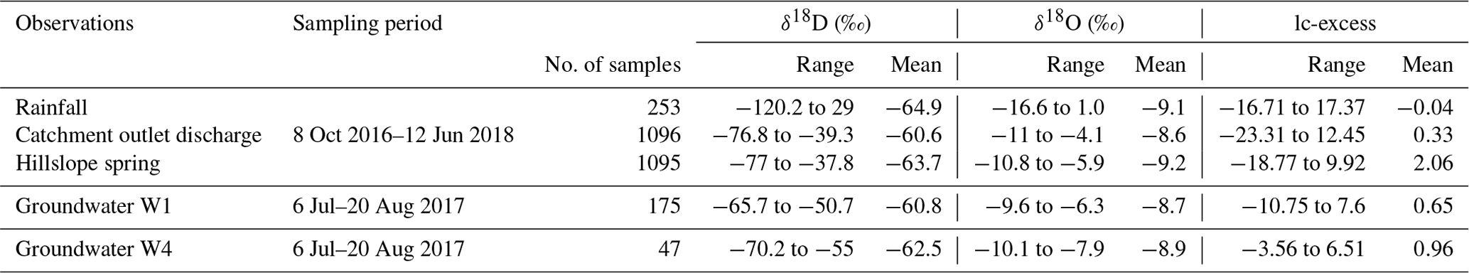
For stable isotope analysis, the hillslope spring, the catchment outlet flows and rainfall were sampled using an autosampler set. The sampling frequency was daily in the dry season (September–April) and hourly in the rainy season (May–August). In total, we collected 253 rainfall samples, 1095 hillslope spring samples and 1096 water samples at the catchment outlet of the underground channel during the study period (Table 3).

As shown in Fig. 1c, there are two observation wells (W1 and W4) near the catchment outlet and the upstream depression. W1 is located in a locally confined aquifer, consisting of extensively fractured carbonate rock surrounded by rock with low secondary porosity. W4 is located in an unconfined aquifer with the vertical permeability decreasing from a large rock fracture and high secondary porosity to low secondary porosity (Chen et al., 2018). The depression groundwater in the two wells (W1 and W4 in Fig. 1c) was manually sampled. Samples were taken at depths of 35 and 13 m for W1 and W4, respectively, with a sampling frequency of two occasions before and after the four rainfall events from 6 July to 20 August 2017.

The sampled water was sealed by using plastic bags to avoid evaporation. Water samples were taken to the laboratory every day and stored at about 4 ^∘C. The water samples were tested and analyzed by a MAT 253 laser isotope analyzer (instrument precision was ±0.5 ‰ for δD and ±0.1 ‰ for δ¹⁸O) at the State Key Laboratory of Hydrology and Water Resources of Hohai University.

2.4 Characteristics of the observed hydrograph and stable isotope dynamics

The observed surface, subsurface and total outlet flow (discharge) are shown in Fig. 2. The discharge response to rainfall is rapid, characterized by a sharp rise and decline in hydrographs. During the study period, the surface flow and underground flow are 43 % and 57 % of the total discharge, respectively. Various lines of evidence have demonstrated the hillslope–depression fast-flow connection, particularly during heavy-rainfall events. In the mid-season, after extremely heavy rainfall, hillslope spring discharge is highly synchronized with outlet flow, and the relationship between hillslope spring discharge and outlet discharge approaches a monotonic function (details in R. Zhang et al., 2020). It is worth noting that, due to the impact of agricultural irrigation, there were unreasonable sudden declines in surface and subsurface flow in June.

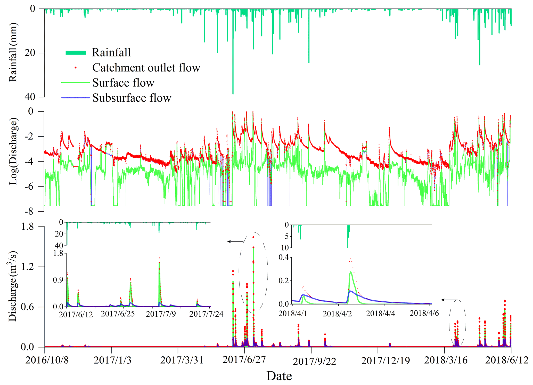
Figure 2 The observed surface, subsurface and catchment total outlet flow (discharge) during the study period.

The mean values of δD and δ¹⁸O (Table 3) clearly show that the isotopic composition of water in the catchment becomes more enriched from the hillslope spring to the depression groundwater and the catchment outlet discharge. This implies increased mixing with more enriched groundwater affected by evaporative fractionation over the course of water flow paths from the hillslopes towards the outlet (Zhang et al., 2019; R. Zhang et al., 2020). This is also illustrated by the fact that the δD–δ¹⁸O regression lines for hillslope spring and outlet discharge deviate from the local meteoric water line (LMWL) (δD = 8.18δ¹⁸O + 9.52), as shown in Fig. 3. Additionally, the regression line of hillslope flow is close to that of the catchment outlet discharge, inferring that hillslope flow is a primary source of outlet discharge. The strong connection between hillslope flow and outlet discharge is attributed to the wide spread of the high-permeability zone in depressions (e.g., at W4). The more depleted isotope signals at W4 show that the groundwater there receives more new water (fast flow) from the hillslope spring and rainfall. By contrast, some older water in the less-permeable area of depressions (e.g., at W1) still contributes to the outlet discharge. The more enriched δ¹⁸O and δD values at W1 show that flow there seldom mixes with new water (rainfall) (Chen et al., 2018), which could lead to a marked departure from the LMWL (Fig. 3).

The monthly statistical summaries of δD and lc-excess (lc-excess =δD-a ⋅ δ¹⁸O − β) are shown in Fig. 4. In the wet season, from May to October, δD is gradually depleted, reflecting rainfall inputs; in contrast, in the dry season, from November to April, δD is gradually enriched. This indicates that both the hillslope spring and outlet discharge change from receiving more new rainwater in wet season to being dominated by older water in the dry season. Meanwhile, δD is more depleted and the lc-excess is more positive for the hillslope flow, compared with the outlet discharge. This means that additional flow sources in the depression join the hillslope flow. This depression flow is older but undergoes less evaporation because of the flat topography and thicker soils. Nevertheless, the additional depression flow has little influence on discharge variability at the catchment outlet, as the various patterns of δD and lc-excess at the catchment outlet closely correspond to those of the hillslope spring.

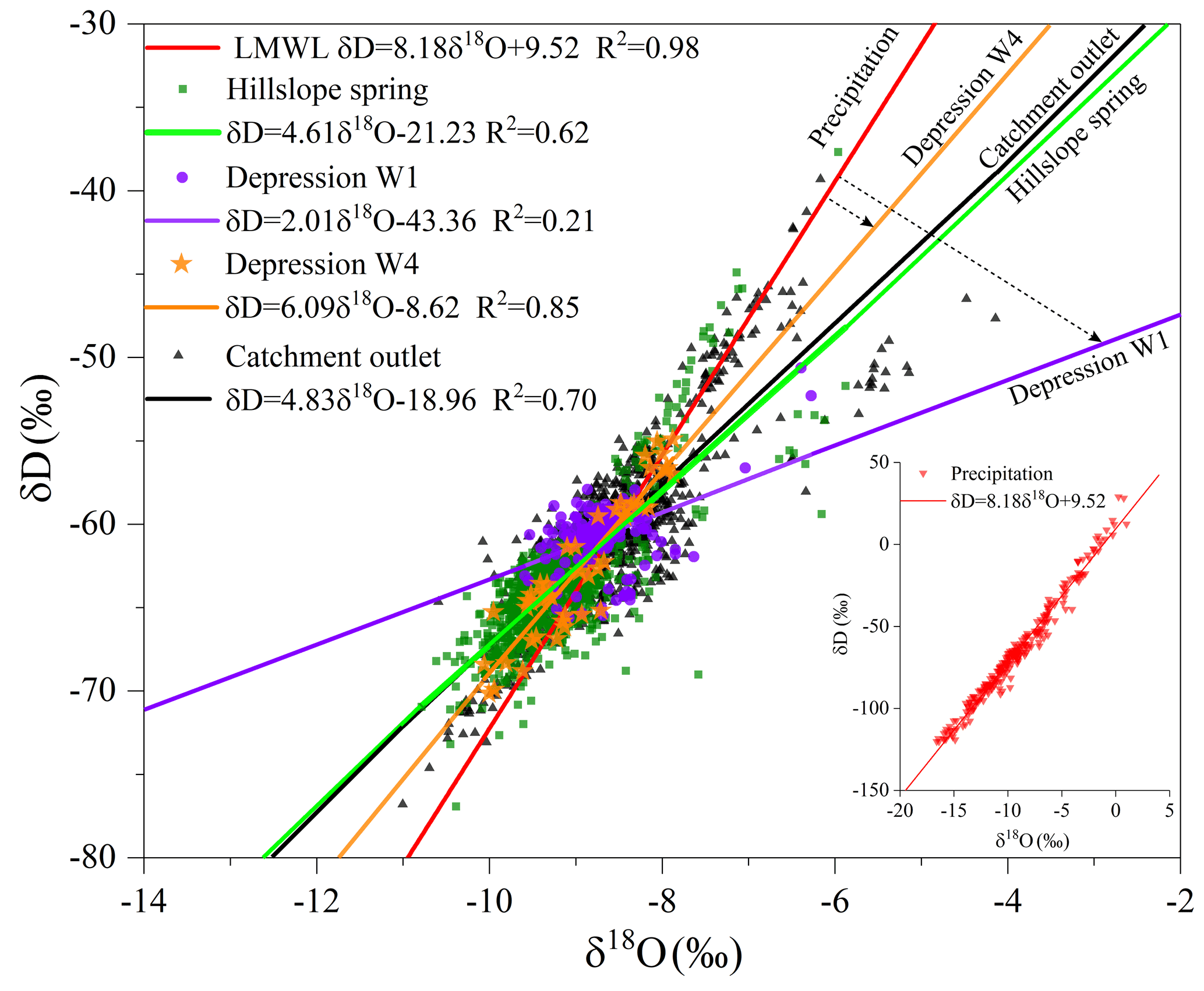
Figure 3 Plot of δ¹⁸O–δD for rainwater, catchment outlet discharge, hillslope spring and depression groundwater at wells W1 and W4. The correlation between δ¹⁸O and δD at W1 is 0.21 (tested to be significant at the significance level of p < 0.001).

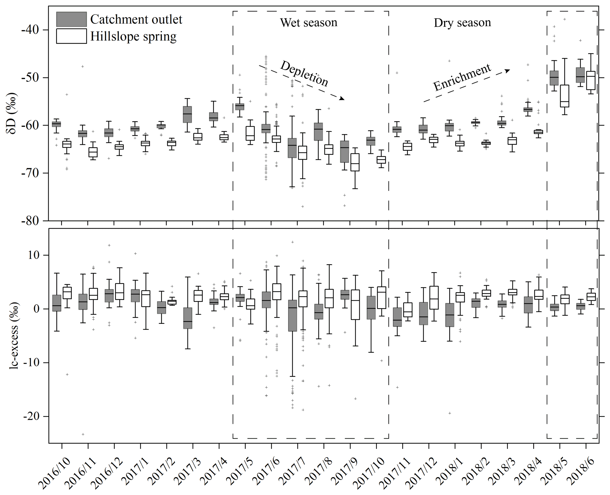
Figure 4 Monthly summaries of observed δD and lc-excess of outlet discharge and the hillslope spring during the study period.

Table 3 Statistical characteristics of isotope data for rainfall, hillslope spring, catchment outlet discharge and depression groundwater during the study period.

3 Model development

3.1 Conceptual model structure

Considering the contrasting features of the catchment landscape, the catchment area is conveniently subdivided into hillslope and depression units, and the model structure can be conceptualized by focusing on the hydrologic connectivity of the “hillslope–depression–stream” continuum (R. Zhang et al., 2020). In each of the hillslope and depression units, the vertical profile is separated into an unsaturated zone, comprising the soil and epikarst layers, and a saturated zone, representing the deep aquifer (Fig. 5). The effect of spatial heterogeneity on hydrological functions is described by a distribution curve of storage in the unsaturated zone, and a dual-flow system in the saturated zone. The distribution curve of storage, like a set of compartments in the VarKarst model (Hartmann et al., 2013), has functions to quantify various recharge mechanisms (e.g., diffusive and concentrated allogenic and autogenic recharge). The dual-flow system consists of a fast-flow reservoir and a slow-flow reservoir that are interconnected and can be used for groundwater routing (Hartmann et al., 2013; Zhang et al., 2019).

The steep hillslope flow moves to the low-lying depression with the following possible connections: hillslope fast flow to depression fast/slow flow (HF–DF/DS), and hillslope slow flow (HS) to depression fast/slow flow (Fig. 5). As hillslope fast flow is primarily concentrated into depression conduits, the connection of HF–DS is neglected in this study.

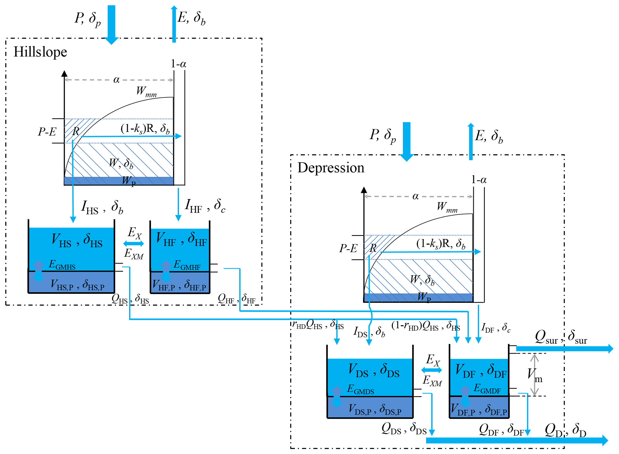
Figure 5 Conceptualized structure for the coupled flow–isotope model. The light blue shades indicate active storage, and the dark blue shades indicate passive storage. Detailed descriptions of the model parameters are given in Table 5.

3.1.1 Hydrological routing

In each of the hillslope and depression units, the spatial heterogeneity of unsaturated storage volumes is described by a distribution curve of the storage capacity, such as the Xinanjiang model in Fig. 5 (Zhao, 1992), following:

$$\begin{array}{}\text{(1)}& {\displaystyle \frac{f}{F}}=\mathrm{1}-{\left(\mathrm{1}-{\displaystyle \frac{W_{{\mathrm{m}}^{\prime }}}{W_{\mathrm{mm}}}}\right)}^b,\end{array}$$

where f represents the free water yield area, F represents the total of the area (α), $W_{{\mathrm{m}}^{\prime }}$ is the areal mean tension water storage at f, W_mm is the maximum value of $W_{{\mathrm{m}}^{\prime }}$ and b is a parameter.

Based on Eq. (1), the initial areal average storage W is an integration of $W_{{\mathrm{m}}^{\prime }}$ within 0−A in the area ($\mathrm{1}-f/F$):

$$\begin{array}{}\text{(2)}& W=\underset{\mathrm{0}}{\overset{A}{\int }}{\left(\mathrm{1}-{\displaystyle \frac{W_{{\mathrm{m}}^{\prime }}}{W_{\mathrm{mm}}}}\right)}^b\mathrm{d}{W}_{{\mathrm{m}}^{\prime }}={\displaystyle \frac{W_{\mathrm{mm}}}{\mathrm{1}+b}}\times \left[{\left(\mathrm{1}-{\displaystyle \frac{A}{W_{\mathrm{mm}}}}\right)}^{\mathrm{1}+b}\right].\end{array}$$

When A=W_mm, the storage in the entire area reaches storage capacity. Thus, the mean storage capacity W_m is equal to $\frac{W_{\mathrm{mm}}}{\mathrm{1}+b}$ (Zhao, 1992).

When the net precipitation (P–E) > 0 and P–E+A < W_mm, the water yield R is

$$\begin{array}{}\text{(3)}& R=P-E-W_{\mathrm{m}}+W+W_{\mathrm{m}}\times {\left(\mathrm{1}-{\displaystyle \frac{P-E+A}{W_{\mathrm{mm}}}}\right)}^{\mathrm{1}+b}.\end{array}$$

Note that P is precipitation, and E is actual evaporation estimated by $E=k_{\mathrm{c}}\times E_{\mathrm{P}}\times \frac{W}{W_{\mathrm{mm}}}$, where k_c is a coefficient of evapotranspiration, and E_P is potential evapotranspiration.

If $P-E+A\ge W_{\mathrm{mm}}$, the water yield R is

$$\begin{array}{}\text{(4)}& R=P-E-W_{\mathrm{m}}+W.\end{array}$$

The water yield R recharges the deep aquifer, which is separated into diffusive recharge I_S and concentrated allogenic and autogenic recharge I_F. The I_S recharges the slow-flow reservoir of the matrix or the small fracture area with a ratio to hillslope or depression area of α (i.e., I_S=k_s × R × α, where k_s is the ratio of water yield into slow-flow reservoir). The I_F is the remaining runoff ((1−k_s) × R × α) and rainfall P falling on the swallow holes (1−α), which directly recharges the fast-flow reservoir (i.e., I_F= P× (1−α) + R × (1−k_s) × α).

Consequently, in the saturated zone, the water balance in the fast and slow reservoirs is

$$\begin{array}{}\text{(5)}& {\displaystyle \frac{\mathrm{d}{V}_{\mathrm{S}}}{\mathrm{d}t}}=I_{\mathrm{S}}-E_{\mathrm{X}}-Q_{\mathrm{S}},\text{(6)}& {\displaystyle \frac{\mathrm{d}{V}_{\mathrm{F}}}{\mathrm{d}t}}=I_{\mathrm{F}}+E_{\mathrm{X}}-Q_{\mathrm{F}}.\end{array}$$

Here, V_S and V_F are storages of the slow- and fast-flow reservoirs, respectively; Q_S and Q_F are discharges from the slow and fast reservoirs, respectively; and E_X is flux between fast-flow and slow-flow reservoirs.

E_X is estimated as the difference in the saturated storages (or water heads) between the fast-flow and slow-flow reservoirs (i.e., E_X =k_e × (V_S−V_F), where k_e is a coefficient of exchange flux between the slow- and fast-flow reservoirs). Q_S and Q_F are estimated according to the linear relationship between storage V and discharge (i.e., Q_S=η_S × V_S, and Q_F=η_F × V_F, where η_S and η_F are outflow coefficients of the slow- and fast-flow reservoirs, respectively).

3.1.2 Isotopic tracer routing

In each of the hillslope and depression units, the isotope mass balance in the unsaturated zone storage can be expressed as

$$\begin{array}{}\text{(7)}& {\displaystyle \frac{\mathrm{d}(W_U\times {\mathit{\delta }}_b)}{\mathrm{d}t}}=P\times {\mathit{\delta }}_p-R\times {\mathit{\delta }}_b-E\times (\mathrm{1}+l_s)\times {\mathit{\delta }}_b,\end{array}$$

where $W_U(W_U=W+W_{\mathrm{P}}$) is the moisture storage consisting of active storage W or mobile water (Sprenger et al., 2017; Sprenger et al., 2018) and passive storage W_P; l_s is the coefficient of evaporation fractionation; and δ_p and δ_b are the stable isotope ratios of rainwater (P) and moisture (and water yield R), respectively. Equation (7) assumes instantaneous mixing of rainwater (P), water yield (R) and soil moisture (W), and complete mixing of the active storage (W) with passive storage (W_P) in the area (α) because soils are very thin.

For the deeper aquifer, the mass balance in the slow- and fast-flow reservoirs is given by

$$\begin{array}{}\text{(8)}& {\displaystyle \frac{\mathrm{d}(V_{\mathrm{S}}\times {\mathit{\delta }}_{\mathrm{S}})}{\mathrm{d}t}}=I_{\mathrm{S}}\times {\mathit{\delta }}_b-E_{\mathrm{XM}}-E_{\mathrm{GMS}}-Q_{\mathrm{S}}\times {\mathit{\delta }}_{\mathrm{S}},\text{(9)}& {\displaystyle \frac{\mathrm{d}(V_{\mathrm{F}}\times {\mathit{\delta }}_{\mathrm{F}})}{\mathrm{d}t}}=I_{\mathrm{F}}\times {\mathit{\delta }}_c+E_{\mathrm{XM}}-E_{\mathrm{GMF}}-Q_{\mathrm{F}}\times {\mathit{\delta }}_{\mathrm{F}}.\end{array}$$

Here, E_XM is the exchange mass between the slow-flow and fast-flow reservoirs (estimated by k_e × (V_S−V_F) × δ_S for E_XM > 0 and by k_e × (V_S−V_F) × δ_F for E_XM ≤ 0); E_GMS and E_GMF represent the mixing of the solute between the active and passive storages for the slow- and fast-flow reservoirs, respectively; and δ_S and δ_F are the stable isotope δ of the slow flow and fast flow, respectively.

As I_F comes from percolation of both unsaturated zone and direct rainfall recharge, the recharge water mass I_F × δ_c is equal to

$$\begin{array}{}\text{(10)}& I_{\mathrm{F}}\times {\mathit{\delta }}_c=P\times {\mathit{\delta }}_P\times (\mathrm{1}-\mathit{\alpha })+{\mathit{\delta }}_b\times R\times (\mathrm{1}-k_{\mathrm{s}})\times \mathit{\alpha }.\end{array}$$

The mass balance of the passive storage (V_P × δ) affected by E_GMS and E_GMF for slow- and fast-flow reservoirs is

$$\begin{array}{}\text{(11)}& {\displaystyle \frac{\mathrm{d}(V_{\mathrm{S},\mathrm{P}}\times {\mathit{\delta }}_{\mathrm{S},\mathrm{P}})}{\mathrm{d}t}}=E_{\mathrm{GMS}},\text{(12)}& {\displaystyle \frac{\mathrm{d}(V_{\mathrm{F},\mathrm{P}}\times {\mathit{\delta }}_{\mathrm{F},\mathrm{P}})}{\mathrm{d}t}}=E_{\mathrm{GMF}}.\end{array}$$

Here, V_S,P and V_F,P are the passive storage of the slow-flow and fast-flow reservoirs, respectively; δ_S,P and δ_F,P are the stable isotope δ of passive storage for the slow-flow and fast-flow reservoirs, respectively; and E_GMS=ϕ_S × V_S × (${\mathit{\delta }}_{\mathrm{S}}-{\mathit{\delta }}_{\mathrm{S},\mathrm{P}})$ and E_GMF=ϕ_F × V_F × (${\mathit{\delta }}_{\mathrm{F}}-{\mathit{\delta }}_{\mathrm{F},\mathrm{P}})$, where ϕ_S and ϕ_F are the exchange coefficient between the active and passive storages for slow flow and fast flow, respectively.

The above Eqs. (8) and (11) describe partial mixing between V_S and V_S,P for the slow-flow reservoir, and Eqs. (9) and (12) describe partial mixing between V_F and V_F,P for the fast-flow reservoir. Moreover, the partial mixing could be static or dynamic depending on whether the exchange coefficients between active and passive storages (ϕ_S and ϕ_F) are constant or vary over time, respectively (Hrachowitz et al., 2013).

3.1.3 Hillslope–depression connectivity and schematic model structures incorporating passive storage

The hillslope fast flow is assumed to fully connect with fast pathways in the depression (i.e., HF–DF in Table 4), whereas the hillslope slow flow passes through both the slow matrix and fast pathways in the depression (i.e., HF–DF/DS in Table 4). Therefore, the storages of V_S and V_F in the depression unit receive additional recharge from the hillslope slow flow. Hence, the hillslope slow- or fast-flow contribution to the depression slow or fast flow is $r_{\mathrm{HD}}\times \frac{A_{\mathrm{H}}}{A_{\mathrm{D}}}\times Q_{\mathrm{S}}$ or $(\mathrm{1}-r_{\mathrm{HD}})\times \frac{A_{\mathrm{H}}}{A_{\mathrm{D}}}\times Q_{\mathrm{S}}+\frac{A_{\mathrm{H}}}{A_{\mathrm{D}}}\times Q_{\mathrm{F}}$, respectively, where r_HD is a ratio of hillslope slow flow into depression slow flow, and A_H and A_D are hillslope and depression areas, respectively. Correspondingly, V_S × δ_S and V_F × δ_F in the depression are influenced by the isotope composition of the hillslope inputs ($r_{\mathrm{HD}}\times \frac{A_{\mathrm{H}}}{A_{\mathrm{D}}}\times Q_{\mathrm{S}}\times {\mathit{\delta }}_{\mathrm{S}}$ and $(\mathrm{1}-r_{\mathrm{HD}})\times \frac{A_{\mathrm{H}}}{A_{\mathrm{D}}}\times Q_{\mathrm{S}}\times {\mathit{\delta }}_{\mathrm{S}}+\frac{A_{\mathrm{H}}}{A_{\mathrm{D}}}\times Q_{\mathrm{F}}\times {\mathit{\delta }}_{\mathrm{F}}$ from the hillslope slow flow and fast flow, respectively).

Table 4 Different model structures that incorporate passive storages into fast-flow and/or slow-flow reservoirs at hillslope and/or depression units.

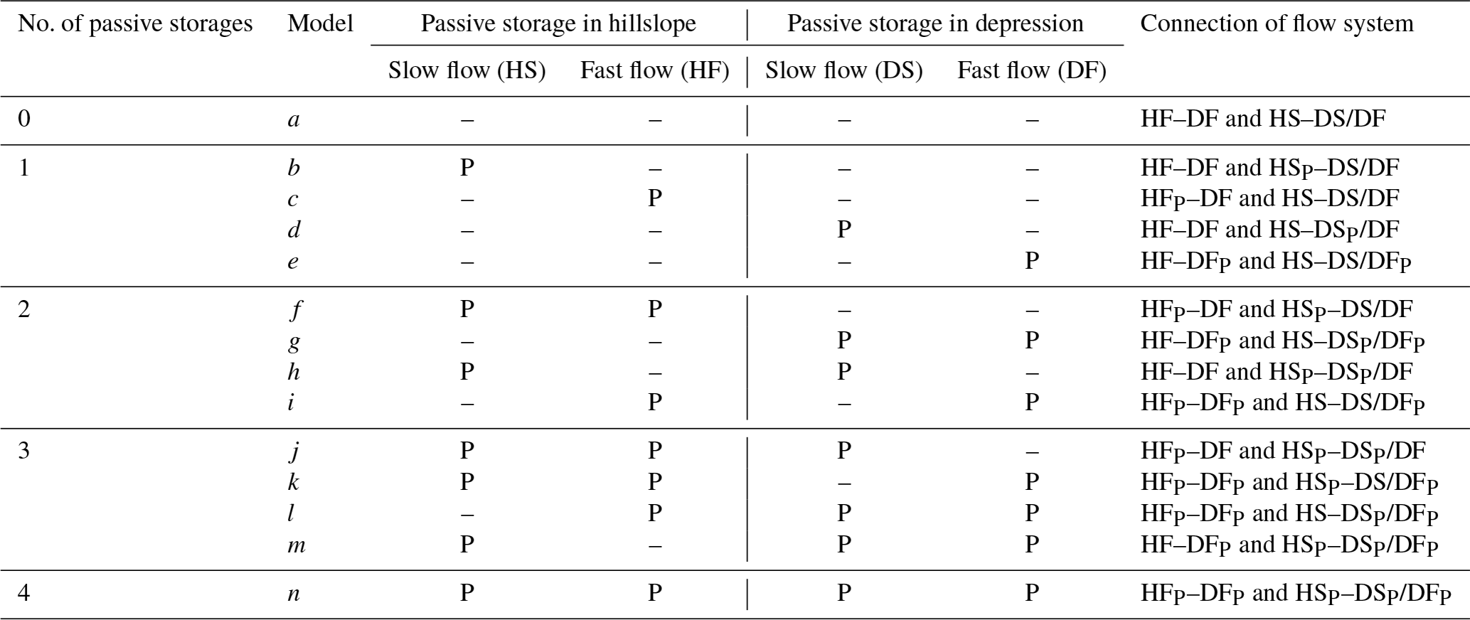
Note that “P” and “–” represent the fast- and slow-flow reservoirs with and without passive storage, respectively.

There is a dual-drainage system, comprising both a surface stream and underground channel, in the depression. Here, we set a critical volume V_m in the depression. The catchment flow drains from the surface stream Q_sur only when the depression groundwater storage meets V_DF > V_m (i.e., $Q_{\mathrm{sur}}=\frac{(V_{\mathrm{DF}}-V_{\mathrm{m}})\times A_{\mathrm{D}}}{\mathrm{\Delta }t}$). As a consequence, the total flow discharge at the catchment outlet Q is composed of fast flow (Q_F) and slow flow (Q_S) in the subsurface, with additional contributions from the surface stream Q_sur.

Passive storage may exist in any flow system (fast and slow flow) or geographical unit (hillslope and depression) in karst catchments (Fig. 5). To optimize the number and positions of passive storage in the flow system, we set 14 schemes (scenarios) that incorporate zero to four passive storages in different positions of the fast and slow reservoirs for hillslope and depression units (indicated by the subscript “P” in Table 4). The model parameters and their definitions are listed in Table 5.

Table 5 The definitions of model parameters with their ranges.

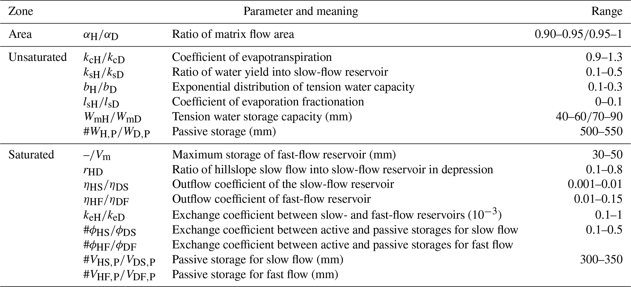
Note that the upper and lower parameters in values separated by “${}^{*}{/}^{*}$” represent the hillslope and depression, respectively. The parameters indicated by “#” refer to those used for isotope concentration simulation. “–” represents not available.

3.2 Model calibration and validation

The observational data were used separately for the calibration and validation periods. More specifically, the model parameters were calibrated against the observed discharge and isotope concentration (δD) from 8 October 2016 to 30 October 2017. Afterwards, the model was validated against observations from 1 November 2017 to 12 June 2018. Note that, as δD and δ¹⁸O fluctuated with virtually the same dynamic over time and both were driven by the same hydrological factors, only δD was used for calibration. The flow–isotope coupled models with different combinations of the active and passive storages (Table 4) were run at hourly time steps.

In this study, the multi-objective optimization algorithm, i.e., the non-dominated sorting genetic algorithm II (NSGA-II) proposed by Deb et al. (2002), was applied for the model parameter calibration. The NSGA-II algorithm (Kollat and Reed, 2006), based on the NSGA algorithm, can identify sets of Pareto-optimal solutions. As Pareto-optimal sets of solutions are not dominated by any one of the factors, as a result of trade-off effects, the “best” solution is achieved by satisfying the demands of the performance objective functions, including the modified Kling–Gupta efficiency (KGE) and the absolute value of the bias (Abias_q) (Fenicia et al., 2007). The KGE criterion comprehensively considers the linear correlation and standard deviation between the numerical and observed values (Kling et al., 2012):

$$\begin{array}{}\text{(13)}& {\mathrm{KGE}}_i=\mathrm{1}-\sqrt{(r-\mathrm{1}{)}^{\mathrm{2}}+(\mathrm{SD}-\mathrm{1}{)}^{\mathrm{2}}+(\mathit{\mu }-\mathrm{1}{)}^{\mathrm{2}}}.\end{array}$$

Here, r is the linear correlation coefficient between the simulated and observed values; SD is the ratio of the standard deviation of the numerical and observed values; μ is the ratio of the average numerical value to the observed value; and $i=(q,c)$ represents the goodness of fit for flow discharge or isotope concentration, respectively. The closer KGE is to 1, the better the overall performance of the coupled model.

The Abias_q is

$$\begin{array}{}\text{(14)}& {\mathrm{Abias}}_q=\mathrm{|}{\displaystyle \frac{\sum _{i=\mathrm{1}}^n(S_i-O_i)}{\sum _{i=\mathrm{1}}^n{O}_i}}\mathrm{|},\end{array}$$

where S_i is the simulated discharge, and O_i is the observed discharge. The closer Abias_q is to 0, the better the performance of the model with respect to matching flow discharge at the outlet.

For a number of iterations (e.g., 1000 in this study), 50 parameter sets were initially retained. The remaining sets with an Abias_q value less than or equal to 0.2 in the 50 parameter sets were then sorted from largest to the smallest according to the sum of corresponding KGE_q and KGE_c. Finally, 30 sets were selected as the Pareto-optimal solution (Nan et al., 2021). The corresponding objective function values (average of the optimal solution sets) for both the calibration and validation periods were extracted.

The range of each parameter value is initially set for model calibration according to our previous investigations (Zhang et al., 2019; R. Zhang et al., 2020; Xue et al., 2019). The volumes of passive storages (W_H,P and W_D,P; V_S,P and V_F,P) are generally 1 order of magnitude larger than those of active storage (Dunn et al., 2010; Soulsby et al., 2011; Ala-aho et al., 2017). Thus, the ranges of W_H,P and W_D,P in the unsaturated zone are set as 500–550 mm, and the ranges of V_H,P and V_D,P in saturated zone are set as 300–350 mm. Considering the rapid hydrological response of the fast-flow system or the hillslope unit to precipitation, the initial values of active storage (V_HF, V_DF and V_HS) are set to 0 mm, whereas the initial value of V_DS is 20 mm (Xue et al., 2019). Meanwhile, the isotope ratios for deuterium are all initially set to the measurement at the catchment outlet (i.e., −61.3 ‰); this initialization contributes negligible errors because isotope transport is driven by the rainfall input boundary condition.

A regional sensitivity analysis (Freer et al., 1996) was executed to identify the most important model parameters. The sensitive parameters targeting KGE_q are the ratio of water yield into the slow-flow reservoir ($k_{\mathrm{sH}}/k_{\mathrm{sD}}$), the maximum storage of the fast-flow reservoir V_m and the outflow coefficient of the fast-flow reservoir in the hillslope unit (η_HF). There are other sensitive parameters when targeting KGE_c, including α_H, k_cH, k_sH, b_H, W_mH and η_HS in the hillslope unit as well as α_D, k_cD and η_DS in the depression unit. Overall, the parameters in the hillslope unit are more sensitive to discharge and isotopic ratios compared with those in the depression unit.

4 Results

4.1 Performance of models during calibration and validation periods

The 30 optimal solutions and their means for the objective functions of KGE_q, KGE_c and Abias_q are obtained from the parameter calibration of 14 models, as shown in Table 6 and Fig. 6. Most models obtain a higher KGE_q but a lower KGE_c, which has also been reported by other studies (Soulsby et al., 2015; Dehaspe et al., 2018; Mudarra et al., 2019; Birkel et al., 2020). For the models incorporating one to four passive storages in Table 4, the accuracy of the simulated discharge and isotopic concentration does not increase with the number of passive storages. Comparatively, models c, f and j give higher mean values for both KGE_q (> 0.65) and KGE_c (> 0.55) (Table 6), and models c and f also obtain a more constrained range of KGE_q and KGE_c from the 30 sets of optimal solutions (Fig. 6) in the calibration and validation periods. All three models showing better performance have a passive storage in the hillslope fast reservoir but do not incorporate any passive storage in the depression fast reservoir (see Table 4). This indicates that hillslope (fast) flow and isotope mixing control catchment outlet discharge and isotopic concentration are consistent with the inferences from the observational data analysis.

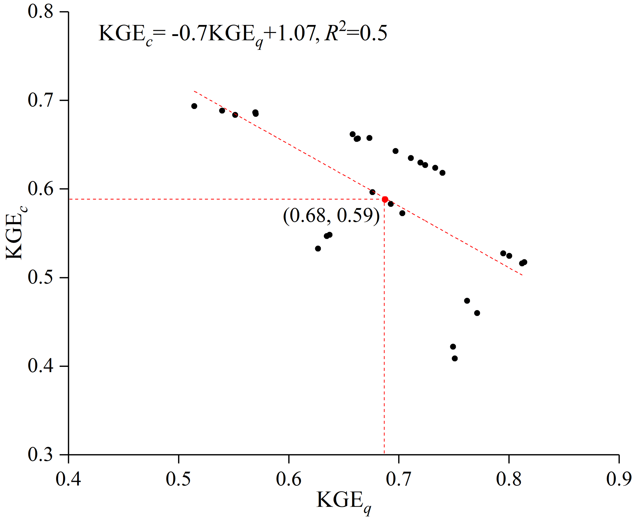
As an example, Figs. 7 and 8 show the respective outlet discharge and isotope (δD) variations simulated by model f. Model f can generally capture the flood peaks (Fig. 7) and the isotope (δD) variations (Fig. 8). The average KGE_q and KGE_c from model f are higher than 0.59 in the calibration and validation periods, and Abias_q is relatively small (Table 6). Figure 9 shows that KGE_q is negatively correlated with KGE_c according to the 30 optimal solution sets from the NSGA-II algorithm. Therefore, the multi-objective calibration gives a pair of high trade-off solution values for both KGE_q and KGE_c for the calibrated model f as well as for models c and j. The other models do not balance the trade-off between KGE_c and KGE_q as effectively. For example, model n, with four passive storages, obtains a high KGE_q (> 0.6) but low KGE_q (< 0.3) (Table 6).

Table 6 Model performance based on the average of 30 optimal solution sets for each individual model structure.

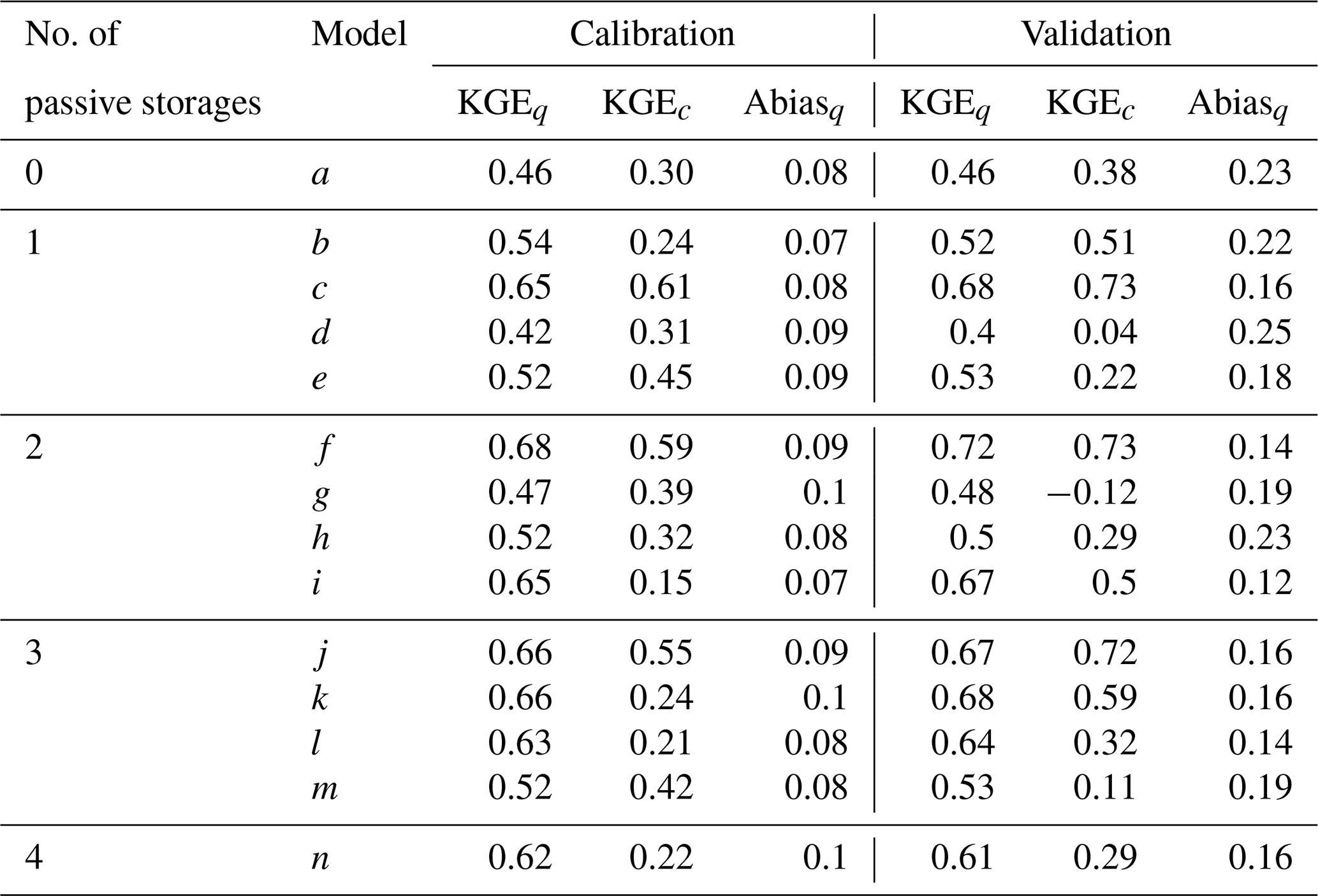
Figure 6 A box plot of the 30 optimal solutions for the objective functions of KGE_q, KGE_c and Abias_q obtained from the parameter calibration of 14 models.

Figure 7 Simulated discharge concentrations of the 30 sets of optimal solutions by model f in the calibration and validation periods. Note that the blue shades represent the simulated range of the 30 optimal solution sets, and the black dots represent the observed discharge (the total of surface and subsurface discharge) at the catchment outlet.

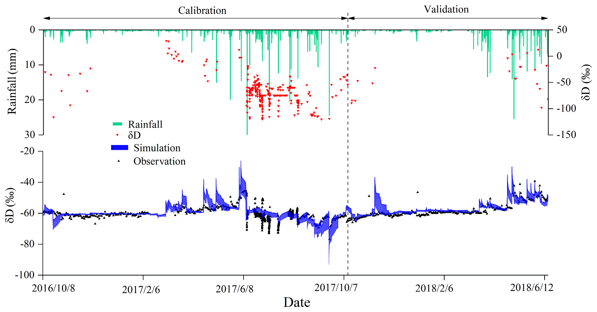
Figure 8 Simulated isotope concentrations of the 30 sets of optimal solutions by model f in the calibration and validation periods. Note that the blue shades represent the simulated range of the 30 optimal solution sets, and the black dots represent the observed isotope concentrations at the catchment outlet.

Figure 9 Relationship between KGE_q and KGE_c from the 30 optimal solution sets of model f.

4.2 Calibrated parameter values

The calibrated parameter values for the models with better performance, models c, f and j, are listed in Table 7. These parameter values reasonably delineate the hydrological features of karst landforms. For example, the calibrated k_s ranges from 0.13 to 0.24 in hillslope and depression units, suggesting that about 76 %–87 % of the net precipitation recharges the fast-flow reservoir through large fractures and sinkholes in terms of $I_{\mathrm{f}}/R=$ (1−α)$P/R+$(1−k_s)α. This high percentage is consistent with the numerical results of Zhang et al. (2011), which were independently derived using a distributed model that considered the role of sinkholes in facilitating fast-flow recharge into the aquifer in the studied catchment. Charlier et al. (2012) found that about 60 % of recharge water entered the conduit network (fast channelized flow paths) in a small karst system in the French Jura Mountains. Worthington et al. (2000) also revealed that more than 90 % of total flow is fast-flow component in four typical karst aquifers in Kentucky, USA. W_m, representing the soil moisture retention capacity, ranges from 52 to 58 mm for thin soils over hillslope, but it is substantially smaller than 81–90 mm for thick soils over depressions according to the calibrated results of the three models with better performance. The outflow coefficient of the fast-flow reservoir η_F (0.14–0.15$/$0.01–0.02 for the hillslope/depression) is much greater than that of the slow-flow reservoir η_S (0.002–0.004$/$0.003–0.005), especially for the hillslope unit. This suggests that fast-flow discharge is much more sensitive to active storage variability than slow-flow discharge because $Q={\mathit{\eta }}_{\mathrm{S}}\times V$. In addition, the optimized ratio of the hillslope slow-flow contribution to the depression slow flow r_HD is close for models c and f (0.37 and 0.39, respectively), which are smaller than the 0.55 reported for model j. The larger r_HD value for model j means more hillslope slow-flow allocation to the depression slow-flow reservoir.

Table 7 The mean values of model parameters for the 30 optimal solution sets from the three models with better performance.

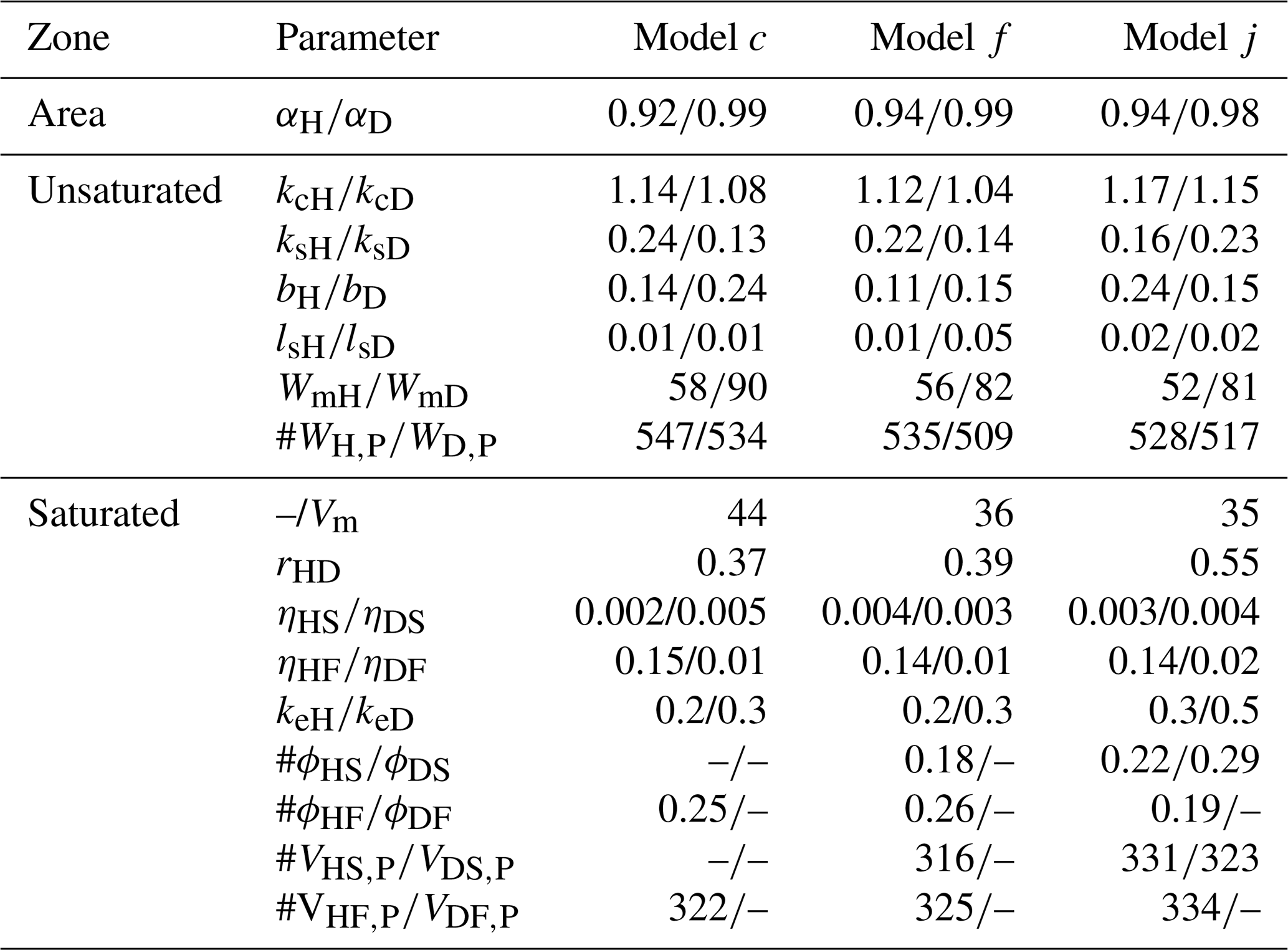
Note that the upper and lower parameters in values separated by “*$/$*” represent the hillslope and depression, respectively. The parameters indicated by “#” refer to those used for isotope concentration simulation. “–” represents not available in the models.

4.3 The effects of passive storage on simulated flow composition and isotopic concentration

We further compared the simulated flow components and their isotopic concentrations for the three models showing better performance (models c, f and j with one to three passive storages in Table 6). The results of model a without any passive storage are also used as a benchmark for comparison. The partitioning of the simulated outlet discharge by the four models is listed in Table 8. All three of the better models with passive stores set in the hillslope unit have a high proportion of discharge from the fast-flow system, particularly in the hillslope unit. In the hillslope unit, model a obtains 79 % of the fast-flow component and 21 % of the slow-flow component, while the three better models with passive stores in the hillslope give a higher proportion of discharge from the fast-flow system (87 %). In the depression unit and at the catchment outlet, the simulated slow-flow composition is slightly different, while the simulated proportions of the underground fast flow and surface flow are largely different in the three models. As shown in Table 8, model f gives 44 % of surface streamflow and 56 % of underground channel flow (the total of fast and slow flow), which are close to observed values at the surface stream (43 %) and underground channel (57 %) outlets. By contrast, models a, c and j (particularly model a) underestimate surface streamflow and overestimate underground channel flow.

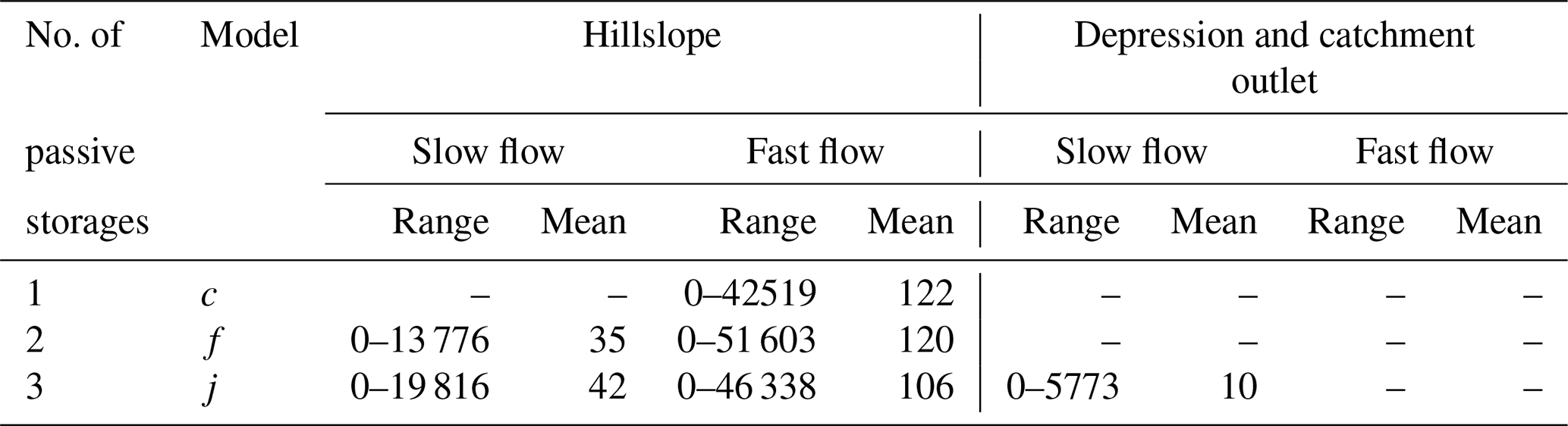
The simulated isotope values of the flow components in the hillslope–depression–outlet continuum are listed in Table 9. Compared with model a, models c, f and jwith passive storages increase isotope mixing and lead to a reduction in the δD variability (see the narrower range of δD for models c, f and j in Table 9). Meanwhile, as the number of passive storages increases in the models, the mixing of the fast flow and slow flow is enhanced, leading to the mean δD values of slow flow approaching that of fast flow. Nevertheless, for the three better models, the strengthened mixing of slow flow only has a limited effect on the mean δD of fast flow, as the mean δD of the catchment outlet flow is closer to that of fast flow. This further supports the hypothesis that hillslope fast-flow dynamics control the catchment flow and isotopic concentration at the outlet.

Table 8 The proportions of flow components in the hillslope–depression–outlet continuum for the 30 optimal solution sets of the selected representative models during the study period ( %).

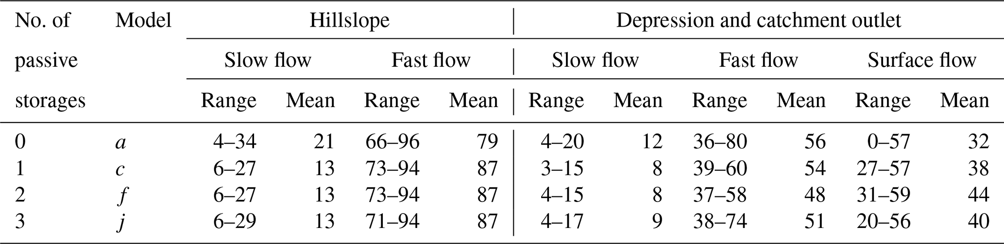
Note that the total flow at the catchment outlet is the sum of slow flow, fast flow and surface flow.

Table 9 The simulated isotope values (‰ ) of flow components in the hillslope–depression–outlet continuum for the 30 optimal solution sets from the selected representative models during the study period.

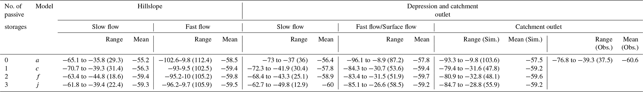
The numbers in parentheses refer to the range of δD.

5 Discussion

5.1 The importance of passive storage for tracer-aided hydrological modeling

Involving passive storage in a coupled flow–isotope model helped to improve the performance of the discharge simulations while also allowing one to capture tracer dynamics, which has been demonstrated by most previous studies (see Table 1). However, the exact configuration of how passive storage is involved in the model can be set in different positions in different models (Table 1) or even in a specific model. Using the STARR (Spatially Distributed Tracer- Aided Rainfall–Runoff) model as an example, van Huijgevoort et al. (2016), Dehaspe et al. (2018) and Piovano et al. (2019) added two passive storages for the soil and groundwater stores, whereas Ala-Aho et al.(2017) and Piovano et al. (2020) only used a passive storage in the soil store. Of all the studies listed in Table 1, only Fenicia et al. (2008) and Birkel et al. (2011b) compared the simulation effects of the model structure on discharge with and without passive storages.

Most previous studies have focused on non-karst catchments, and passive storages are usually represented in slow-flow reservoirs (Hrachowitz et al., 2013; Yang et al., 2021; see Table 1). Birkel et al. (2011a) and Hrachowitz et al. (2013) suggested that this passive storage can be interpreted as soil moisture below field capacity or groundwater below the dynamic storage. For more complex model structures, delineating flow components and connections in heterogeneous landscape units usually requires more flow routing compartments and, thus, additional passive storages. For example, Capell et al. (2012) identified that only three passive storages were necessary for a tracer-aided model with four possible passive storages in upland and lowland units in the North Esk Catchment in northeastern Scotland. They found that passive storage in the shallow zone for the upland unit was negligible, as sufficient damping was available in the dynamic (active) storage.

Required model structures are usually more complex in karst catchments due to different conceptualization of recharge and flow mechanisms. Most studies have demonstrated that the fast channelized flow paths control the sharp rise and decline in the hydrograph; thus, setting passive storage in the fast-flow reservoir can improve simulation accuracy of the catchment flow and tracer dynamics in karst catchments, particularly in cockpit karst landscapes. For example, Zhang et al. (2019) assumed that hillslope flow is rapid, and they showed that directly setting a passive storage in the hillslope flow reservoir can successfully capture the dynamics of flow discharge and stable isotopes in the same study catchment. Similarly, elsewhere, Chang et al. (2020) developed a model capturing the functioning of a dual-flow (fast-flow and slow-flow) system, showing that setting a passive storage in the fast-flow reservoir can reproduce the dynamics of flow discharge and spring EC.

Our study was novel in that we comprehensively analyzed the functioning of alternative configurations of passive storage in a complex model structure for cockpit karst catchments, based on a comparison of the performances of 14 different models. Through this comparison, we demonstrated that adding passive storage in the fast-flow reservoir in the hillslope unit is more efficient for simulating flow components and isotope dynamics, with three alternative choices to set passive storages in our developed model. The most parsimonious model is to add a passive storage in the hillslope fast-flow reservoir, as in model c. The “best” model is to add two passive storages in the fast-flow and slow-flow reservoirs of the hillslope unit, as is the case in model f. This best model can appropriately estimate flow components in addition to the total discharge and isotope concentration at the catchment outlet. Adding an additional passive storage in the depression slow-flow reservoir, such as in model j, does not further substantially increase the simulation accuracy, even though the model obtains higher KGE_q and KGE_c, as shown in Table 6.

5.2 The dominant transport processes: advection, dispersion or molecular diffusion?

Generally, the transport process is largely controlled by advection (with the tracer traveling with water), by molecular diffusion in the slow-velocity (or immobile) zone and by hydrodynamic dispersion in the fast-velocity (or mobile) zone (Karadimitriou et al., 2016; Schumer et al., 2003; Wang et al., 2020). In karst flow systems, larger fractures and conduit media have permeabilities that can be several orders of magnitude higher than those of matrix flow in micropores. In cockpit karst catchments, the hillslope unit has a higher flow velocity but longer flow paths to the outlet. Tracers input farthest from the stream at the hillslope unit will undergo more dispersion (Kirchner et al., 2001). In our study catchment, the hillslope unit has a higher flow velocity, as the outflow coefficient of fast flow in the modeled hillslope unit is much greater than that of the depression unit (Table 7) for the models showing the best performance (c, f and j). Meanwhile, configuring passive storage in the hillslope fast flow alone is sufficient to damp the δD variability effectively. This points to the fact that hydrodynamic dispersion dominates the chemical mixing. Indeed, the dominance of hydrodynamic dispersion has been widely reported in flow-conductive (preferential flow) zones (Roubinet et al., 2012). For example, Zhao et al. (2019, 2021) used a transient storage model (TSM) to study the tailing of breakthrough curves (BTCs) of tracers in karst conduits, with experimental results suggesting that the dispersion coefficient was positively correlated with the flow velocity.

Table 10 The simulated $\left|E_{\mathrm{GM}}\right|$ (m³ ×  ‰) of flow components in the hillslope–depression–outlet continuum for the 30 optimal solution sets from the selected representative models during the study period.

“–” represents not available.

The mass exchange fluxes (E_GMF and E_GMS in Eqs. 11 and 12) between active and passive storages are given in Table 10. The mass exchange flux of hillslope fast flow is greater than that of slow flow, and it is over 10 times larger than that of slow flow in the depression unit. This result also supports the fact that the hillslope unit has stronger dispersion effects. Therefore, the stronger variations in discharge and isotopes can only be better captured simultaneously when the functioning of the advection and dispersion of the hillslope unit is incorporated in the models.

5.3 Uncertainties in adding passive storage in the tracer-aided hydrological modeling

Our model uses a distribution curve of unsaturated storage capacity to describe the spatial heterogeneity of storage volumes, and it employs fast-flow and slow-flow systems to conceptualize dual-karst-flow systems on a large scale (e.g., hillslope and depression units). Optimizing the number of storages balances the need to minimize model complexity and uncertainty while also improving the simulation performance of both flow and tracers. Particularly for karst catchments, this optimization needs to be based on short-time-interval observation data, such as hourly data in our study catchment, to capture the rapid hydrological response. Only such fine-resolution data can capture the dramatic variability in the hydrograph and tracer dynamic and, thus, can be used to successfully optimize the model structure. Nevertheless, the optimized passive storages and model structures are not unique, as the three better models with one to three passive storages performed similarly well in the study catchment, in terms of the catchment input–output responses.

These uncertainties imply that additional observations are needed to enhance our ability to constrain complex model structures and the ranges of model parameters in karst catchments. These additional observations should include not only the catchment input–output responses but also some key hydrological internal state components and their isotope concentrations, such as water fluxes and isotope transport in micropore, fracture and conduit media in karst catchments. Moreover, detailed observations of human activities are also important to reduce the modeling uncertainties. As shown in our study catchment, the depression is occupied by agricultural land. Groundwater pumping for agriculture use causes sudden declines in streamflow and isotopic concentrations in June, as shown in Fig. 7, which makes that the model overestimates low flow.

Our study catchment at Chenqi is broadly representative of extensive regions of headwater catchments in cockpit karst landscapes, and while the model parameters still need to be calibrated for specific catchments, the model is generic and transferable to other areas. The approach also has the potential to be used in upscaling to large catchments, although the model would then need to incorporate river and channel routing, as these play an important role in regulating streamflow variations at larger scales.

6 Conclusions

In cockpit karst landscapes dominated by poljes and surrounding tower areas, depression areas are interconnected with isolated towers scattered throughout the terrain (Lyew et al., 2007). In this study, we developed and tested a coupled flow–tracer model for simulating discharge and isotope signatures for cockpit karst landscapes, represented using a “hillslope–depression–outlet” continuum. We tested 14 simulation cases with alternative model structures by varying the number and configuration of passive storage in the fast-/slow-flow reservoirs of hillslope/depression units. The model structures and parameters were optimized using a multi-objective optimization algorithm to match the observed discharge and isotope dynamics in the Chenqi Catchment in southwestern China.

We found that, for complex models developed for cockpit karst catchments, capturing the main hydrological flow paths and organizing passive storages in relation to these flow paths can efficiently improve model performance. In the Chenqi Catchment, the main hydrological pathways are hillslope flow and its connection with the catchment outlet. The models with one to three passive storages achieve similarly optimal results that are supported by the KGE_q, KGE_c and Abias_q values. All three models have a passive storage in the dominant flow domain (hillslope fast flow).

The optimal model structure is supported by the simulated discharge and tracer dynamics. The hillslope fast-flow system contributes about ∼ 80 % of the outlet discharge. The passive storages in the optimal models strengthen isotope mixing and, thus, constrain the δD and discharge variability. Further comparison of the simulated results by the three optimal models with one to three passive storages showed that the “best” model structure is to incorporate two passive storages in the fast- and slow-flow reservoirs of the hillslope unit. This best model can appropriately estimate flow components in addition to the total discharge and isotope fluctuations at the catchment outlet.

Characterizing the dynamics of flow paths and connections in complex geological settings karst landscapes is central to better understanding fluid flow and solute transport processes. This study provided evidence that the protection of hillslope environments is significant for the prevention of natural hazards, such as droughts, floods and contamination, in karst landscapes.