Improved understanding of regional groundwater drought development through time series modelling: the 2018–2019 drought in the Netherlands

The 2018–2019 drought in north-western and central Europe caused severe damage to a wide range of sectors. It also emphasised the fact that, even in countries with temperate climates, adaptations are needed to cope with increasing future drought frequencies. A crucial component of drought management strategies is to monitor the status of groundwater resources. However, providing up-to-date assessments of regional groundwater drought development remains challenging due to the limited availability of high-quality data. This limits many studies to small selections of groundwater monitoring sites, giving an incomplete image of drought dynamics. In this study, a time series modelling-based method for data preparation was developed and applied to map the spatio-temporal development of the 2018–2019 groundwater drought in the south-eastern Netherlands, based on a large set of monitoring data. The data preparation method was evaluated for its usefulness and reliability for data validation, simulation, and regional groundwater drought assessment. The analysis showed that the 2018–2019 meteorological drought caused extreme groundwater drought throughout the south-eastern Netherlands, breaking 30-year records almost everywhere. Drought onset and duration were strongly variable in space, and higher-elevation areas suffered from severe drought well into 2020. Groundwater drought development appeared to be governed dominantly by the spatial distribution of rainfall and the landscape type. The time series modelling-based data preparation method was found to be a useful tool to enable a spatially detailed record of regional groundwater drought development. The automated time series modelling-based data validation improved the quality and quantity of useable data, although optimal validation parameters are probably context dependent. The time series simulations were generally found to be reliable; however, the use of time series simulations rather than direct measurement series can bias drought estimations, especially at a local scale, and underestimate spatial variability. Further development of time-series-based validation and simulation methods, combined with accessible and consistent monitoring data, will be valuable to enable better groundwater drought monitoring in the future.

1 Introduction

In the summer of 2018, a severe drought hit large parts of north-western and central Europe. Extremely low precipitation coincided with high temperatures, both breaking multi-decadal records in many places (see Bakke et al., 2020; Philip et al., 2020; Toreti et al., 2019). Recurring drought in summer 2019 and early 2020 worsened the situation in large parts of the area. Drying soils and declining water reserves caused damage to agricultural production and natural ecosystems, problems with drinking water and energy production, and widespread forest fires, among other impacts (Bakke et al., 2020; Bastos et al., 2020; Buras et al., 2020; Philip et al., 2020). The kind of “hot drought” that occurred in 2018–2019 is expected to become more frequent in the future in central and northern Europe (Philip et al., 2020; Toreti et al., 2019).

The Netherlands was one of the countries most hit by these weather extremes (Bakke et al., 2020). The damage was felt mainly in the southern and eastern parts of the country (Van de Velde et al., 2019; Van den Eertwegh et al., 2019; Witte et al., 2020b). In a country traditionally more focused on discharging water surpluses, the drought of 2018–2019 was felt by many water managers as a wake-up call, sparking a widespread search for solutions to prepare water systems for increasingly frequent drought extremes (De Lenne and Worm, 2020; IenW, 2019; Witte et al., 2020a; Van de Velde et al., 2019). In the south-eastern Netherlands, as in many other parts of the world, groundwater is a crucial water source. Accordingly, much of the damage in 2018 was directly related to deep declines in groundwater levels (LCW, 2020). Among other effects, the groundwater shortages caused severe damage in peatland and brook ecosystems (Witte et al., 2020b) as well as concerns over the sustainability of increased irrigation and drinking water abstractions (Van de Velde et al., 2019; Van den Eertwegh et al., 2019). Groundwater is often the most persistent water store in the landscape, reacting latest as a meteorological drought propagates into the hydrological system (Van Loon, 2015). This makes proper management of the groundwater a crucial component of drought management strategies.

Previous studies have shown that the response of groundwater to meteorological drought can vary strongly in space. Variations in groundwater response are caused by differences in geology, water management, and other catchment characteristics (Bloomfield et al., 2015; Hellwig et al., 2020; Peters et al., 2006; Van Loon and Laaha, 2015). Therefore, to be able to mitigate and prevent drought damage, it is essential to understand how groundwater drought develops in both time and space. In recent years, water managers in the Netherlands have indeed expressed the need for more up-to-date, location-specific drought information and predictions to be able to take appropriate measures (IenW, 2019; Pezij et al., 2019; Witte et al., 2020a).

Multiple recent research efforts have aimed at better understanding the variations in groundwater drought and its impacts at national and European scales (Bakke et al., 2020; Hellwig et al., 2020; Margariti et al., 2019; Van Loon et al., 2017; Brauns et al., 2020). The 2018(–2019) drought in Europe has so far been studied at larger scales from a meteorological perspective (Bakke et al., 2020; Philip et al., 2020; Toreti et al., 2019) as well as from a hydrological perspective in Scandinavia and Switzerland, among others (Bakke et al., 2020; Brunner et al., 2019). For the Netherlands, some assessments of the drought with respect to groundwater have been made based on small numbers of measurement sites and physically based modelling studies (Van den Eertwegh et al., 2019). However, a more detailed image of how the 2018–2019 drought manifested itself in the groundwater and how this varied in space, based on measurement data, is still lacking. This could provide valuable insights into groundwater drought dynamics and mitigation options in the Netherlands and similar groundwater-dominated lowland regions.

Groundwater heads are widely monitored in observation wells. However, analysis of groundwater drought from these data over large areas is often challenged by data quantity or quality (Kumar et al., 2016). Firstly, data usually have to be obtained from multiple organisations, and they contain errors and other perturbations. Secondly, the length of measured time series is often not sufficient for drought analysis, for which at least 30-year series are recommended (Link et al., 2020). As a result, many groundwater drought studies have focused on relatively few measurement wells with near-natural, long series or on simplified proxies (Bakke et al., 2020; Van Loon et al., 2017; Van den Eertwegh et al., 2019; Kumar et al., 2016). This may give an incomplete image of the true variability in drought dynamics. In addition, the available data usually lag behind the present, hindering the up-to-date drought assessments that water managers need.

To deal with these challenges, several studies have developed methods for automated validation and lengthening of groundwater head time series (Marchant and Bloomfield, 2018; Peterson et al., 2018; von Asmuth et al., 2012). This is usually done with various types of statistical models (Peterson et al., 2018; Van Loon et al., 2017). One type of statistical modelling that has proven very useful for groundwater data is time series modelling with impulse-response functions (Bakker and Schaars, 2019; von Asmuth et al., 2002). These models describe groundwater head variations at a specific location as a function of driving variables, usually weather data, and a fitted impulse-response function. This type of impulse-response time series modelling (TSM) allows accurate simulations to be made without the need for information on site characteristics. The simulations can be used to identify errors and other atypical behaviour in the data as well as to lengthen and harmonise time series, as shown by studies such as Zaadnoordijk et al. (2019), Bartholomeus et al. (2008), and Marchant and Bloomfield (2018). As such, TSM can enable drought studies to use more observation points and to perform real-time monitoring, without the need for a complex physically based model. Marchant and Bloomfield (2018) were the first to develop a full time series model-based method to study groundwater drought over a large region in the UK. Although TSM-based analyses appear to be a valuable tool for groundwater drought assessment, their wider applicability for various cases has not yet been well explored. To be able to widely use TSM data preparation for drought studies, several questions need to be answered.

Figure 1 The study area, showing (a) elevation (AHN, 2019) and (b) soil types (WUR, 2006). The higher-elevation limestone–loess hill landscape in southern Limburg (LLH) and glacier-pushed sand ridges (GPR) are indicated.

Firstly, it is not yet clear which methods are optimal for groundwater data validation. Raw groundwater data sets are usually strongly influenced by errors and disturbances, which can hamper the reliability of analyses such as model calibration and calculation of groundwater characteristics (Post and von Asmuth, 2013; Peterson et al., 2018; Ritzema et al., 2018). Time series modelling can be used to identify time series influenced by disturbances after analysis (e.g. Marchant and Bloomfield, 2018) but also to remove irregularities from the data beforehand. In addition, TSM-based data cleaning can be combined with other more basic consistency checks, improving its effectiveness (Peterson et al., 2018). This validation method has not yet been evaluated for the case of groundwater drought analysis.

Secondly, the reliability of time series simulations for groundwater drought analysis has not been properly tested. To understand the added value of using TSM data preparation, the gain in spatial and temporal cover needs to be balanced with a potential loss of information by cleaning and simulation. Researchers have often used TSM simulations directly as replacement of the data. This may be justified, as these simulations often have a very good fit to observations (Bakker and Schaars, 2019; Zaadnoordijk et al., 2019); however, this approach inevitably also strips out part of the external influences that are not explicitly included in the model drivers (Peterson et al., 2018; Zaadnoordijk et al., 2019). Drought occurrence and development can be strongly affected by human impacts as well as by local-scale natural influences, such as surface water influence (Margariti et al., 2019; Van den Eertwegh et al., 2019). As such, excluding such external drivers of groundwater levels may provide an incomplete image of drought dynamics (Van Loon et al., 2016). In addition, models may have intrinsic difficulties to correctly represent groundwater behaviour during extreme drought conditions, which may cause deviating soil and groundwater flow processes (Hellwig et al., 2020; Avanzi et al., 2020). This is especially important when time series models are used for “nowcasting” groundwater observation series. Under extreme drought conditions, this (by definition) involves modelling system conditions not present in the calibration period and may give incorrect results. Therefore, it is important to understand how the use of TSM simulations rather than measurement series affects the assessment of drought behaviour.

Given these knowledge gaps, the current study aims to evaluate the usefulness of a time series modelling-based data preparation method for regional analysis of groundwater drought. A method is developed consisting of data validation, simulation, and drought assessment (Sect. 3) and is applied to the 2018–2019 groundwater drought in the south-eastern Netherlands in order to characterise its development and recovery in time and space (Sect. 4). The usefulness of the method is evaluated by its performance and reliability with regard to groundwater data validation and simulation as well as by its added value for the resulting regional drought assessment (Sect. 5).

2 Study area and data

The study area covers roughly the south-eastern half of the Netherlands (Fig. 1). This is a low-topography area above sea level, dominated by Pleistocene deposits. The study area has mainly sandy sediments at the surface but is also partially covered by river clays and loess deposits (Fig. 1b). The elevation is mostly between 0 and 30 m above mean sea level, with locally higher areas (Fig. 1a). Higher elevations occur in the limestone–loess hill landscape of southern Limburg and on glacier-pushed ridges in Utrecht and Gelderland (areas indicated in Fig. 1a). Land use is dominated by agriculture, while the glacial ridges are covered mainly with forest. The area has a temperate climate with a yearly precipitation surplus (precipitation of 700–950 mm yr⁻¹ and reference evapotranspiration of around 600 mm yr⁻¹). In addition, the groundwater system is affected by abstractions for drinking water and irrigation as well as by drainage systems in the lowest-lying parts of the study area.

Figure 2 Method workflow.

Groundwater head data were supplied by several regional water managing bodies. For some areas, additional series were obtained from the Dutch national groundwater database DINO (TNO, 2022). The data consist of groundwater head time series with a bimonthly to sub-daily frequency, mostly running until spring 2019. In addition, metadata of the monitoring wells were available, including location, filter depth, and surface level. Only data from the first filter of boreholes were used, generally representing the phreatic level. Those series were selected that contained ≥10 years of data, to ensure sufficient data for time series model fitting (see Zaadnoordijk et al., 2019), and that ended after 31 August 2018. The 2018–2019 meteorological drought peaked in summer 2018; therefore, summer 2018 was chosen as the focus period for model evaluation. This resulted in 2722 series for further analysis.

Daily precipitation (P) and reference evapotranspiration (ET_ref) were obtained from the Royal Netherlands Meteorological Institute (KNMI) for January 1990 to May 2020 (KNMI, 2020). Data were used from 15 general weather stations (for ET_ref) and 114 precipitation stations distributed homogeneously over the study area. Reference evapotranspiration is determined by KNMI following Makkink (1957). The ET_ref series did not always cover the full period of interest; gaps were filled with the nearest station that did have full data (maximum distance of around 50 km).

3 Methods

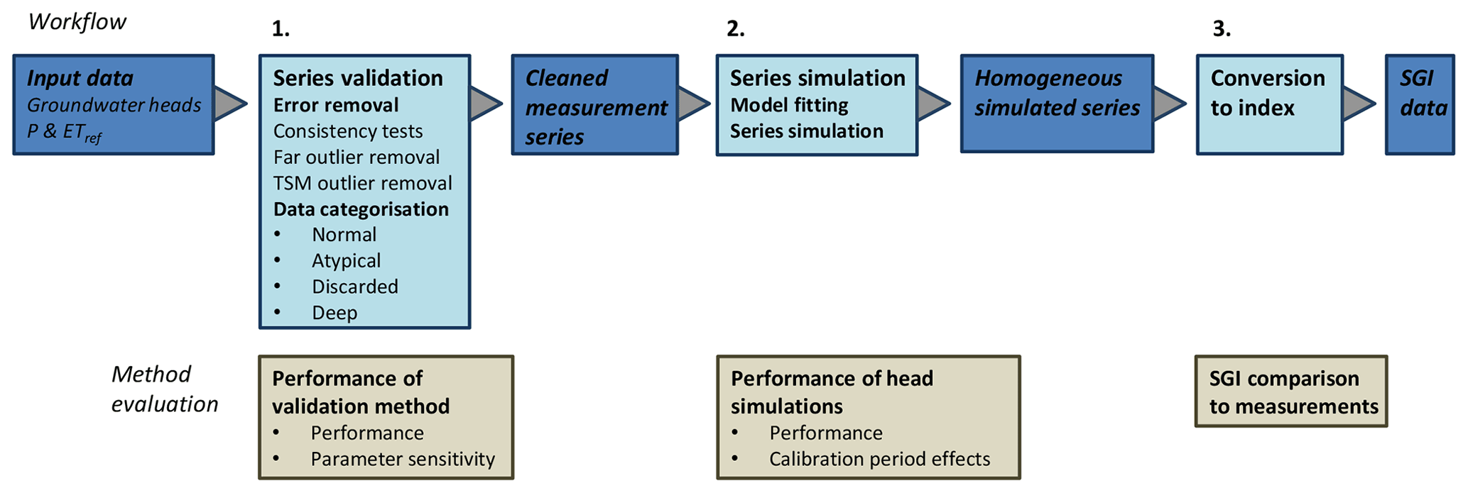
The method for data preparation and drought analysis consists of three components (Fig. 2): (1) validation of the observed groundwater heads, (2) simulation of groundwater heads, and (3) conversion to a standardised groundwater index (SGI). Each step is evaluated by one or more tests. In addition, the resulting drought assessment for the case study region is explored as an example of a regional-scale application.

3.1 Time series modelling method

This study has made use of time series modelling with predefined impulse-response functions, as developed by von Asmuth et al. (2002). Time series modelling was done with the Pastas package for Python developed by Collenteur et al. (2019). The used model set-up largely follows Collenteur et al. (2019) and is described in more detail in Appendix A. In short, groundwater levels (GWL) were simulated as a base level d, overlain by a temporal fluctuation in response to external stresses – in this case only recharge. Here, recharge is estimated as follows:

$$\begin{array}{}\text{(1)}& R\left(t\right)=P\left(t\right)+f\cdot {\mathrm{ET}}_{\mathrm{ref}}\left(t\right),\end{array}$$

where f is a calibration parameter. The use of the linear recharge model of Eq. (1) is a simplification that may not be optimal for all locations in this study (Collenteur et al., 2021; Bakker and Schaars, 2019). However, as linear recharge models have been successfully applied in many cases in the Netherlands (e.g. Zaadnoordijk et al., 2019; von Asmuth et al., 2012) and as we aimed to explore the potential of impulse-response time series modelling for drought studies rather than to compare different model set-ups, we chose to use the simplest model set-up possible (see Sect. 5.1.2 for further comments).

The response of groundwater to a recharge impulse is modelled by a scaled gamma function as in von Asmuth et al. (2002) and Collenteur et al. (2019) (see Appendix A). The variation in groundwater heads over time is calculated by convolution of this impulse-response function with the recharge time series.

This gives five parameters to be calibrated for each individual location. Parameter A represents the long-term response of the groundwater level to a constant recharge input of one unit, in this case 1 mm d⁻¹; a and n determine the shape of the recharge response function; f is the influence of ET_ref relative to precipitation; and d is the groundwater base level. For purposes of parameter calibration, an exponential noise model is also fitted to the residuals with the additional noise decay parameter α.

Table A1 gives the calibration settings used for each parameter. The default method for parameter optimisation was used, minimising the weighted squared noise using a least squares method (Collenteur et al., 2019).

3.2 Series validation

Raw groundwater data sets are usually strongly influenced by errors and disturbances. Often no information is available on potential sources of deviations, and these have to be identified from the groundwater data themselves (Post and von Asmuth, 2013; Peterson et al., 2018; Ritzema et al., 2018). Phreatic groundwater levels typically follow an annual cycle, overlain by faster fluctuations in response to rainfall and evapotranspiration. An actual series of measured groundwater heads will often show deviations from this expected pattern. Deviations may be of short duration, such as those caused by a typing error, temporary instrument failure, or short-term groundwater abstraction, and can be denoted outliers: a small number of measurements far from the expected level, occurring over a short period (days or weeks) relative to the general (seasonal) fluctuations in most groundwater series (e.g. Peterson et al., 2018). Deviations may also be structural, affecting the series' behaviour over months or longer. These are visible as level shifts, trends, and other abnormal patterns in the data series (see Sect. S1 in the Supplement). Such long-term deviations can be caused by errors, such as instrument drift; however, they can also reflect real groundwater behaviour caused by local natural or human influences, such as surface water influence or abstraction (Post and von Asmuth, 2013; Zaadnoordijk et al., 2019; Margariti et al., 2019). Logbook notes from data collectors available for a small subset of our data set indeed showed frequent disturbances such as short-term abstractions, changes in water management, sensor problems, relocation of wells, well maintenance, and other issues.

To prepare the data for the drought analysis, we used a validation set-up that treats short-term (outliers) and long-term deviations separately. The validation method aims to remove all important outliers: erroneous outliers will lead to incorrect conclusions on the occurrence of extremes, while real short-term disturbances in the groundwater heads are also less relevant for understanding the slow-developing impacts of drought, which is generally considered to occur on timescales of months to years (van Loon, 2015). Erroneous long-term deviations are also undesirable for drought analysis, as these disturb the groundwater level distribution on which drought thresholds are based (see Sect. 3.3). However, real long-term deviations in the groundwater level, such as those caused by long-term abstraction and land use effects, should ideally be retained to capture the real variability in drought behaviour (Van Loon et al., 2016). Whether atypical behaviour in a series is caused by errors or by real external influences is very difficult to distinguish by automated methods. Our approach is, therefore, to classify the series according to their long-term behaviour; this allows for the retention of some of the potentially influenced series in the analysis while also acknowledging their lower reliability.

Table 1 Parameters used for the series validation.

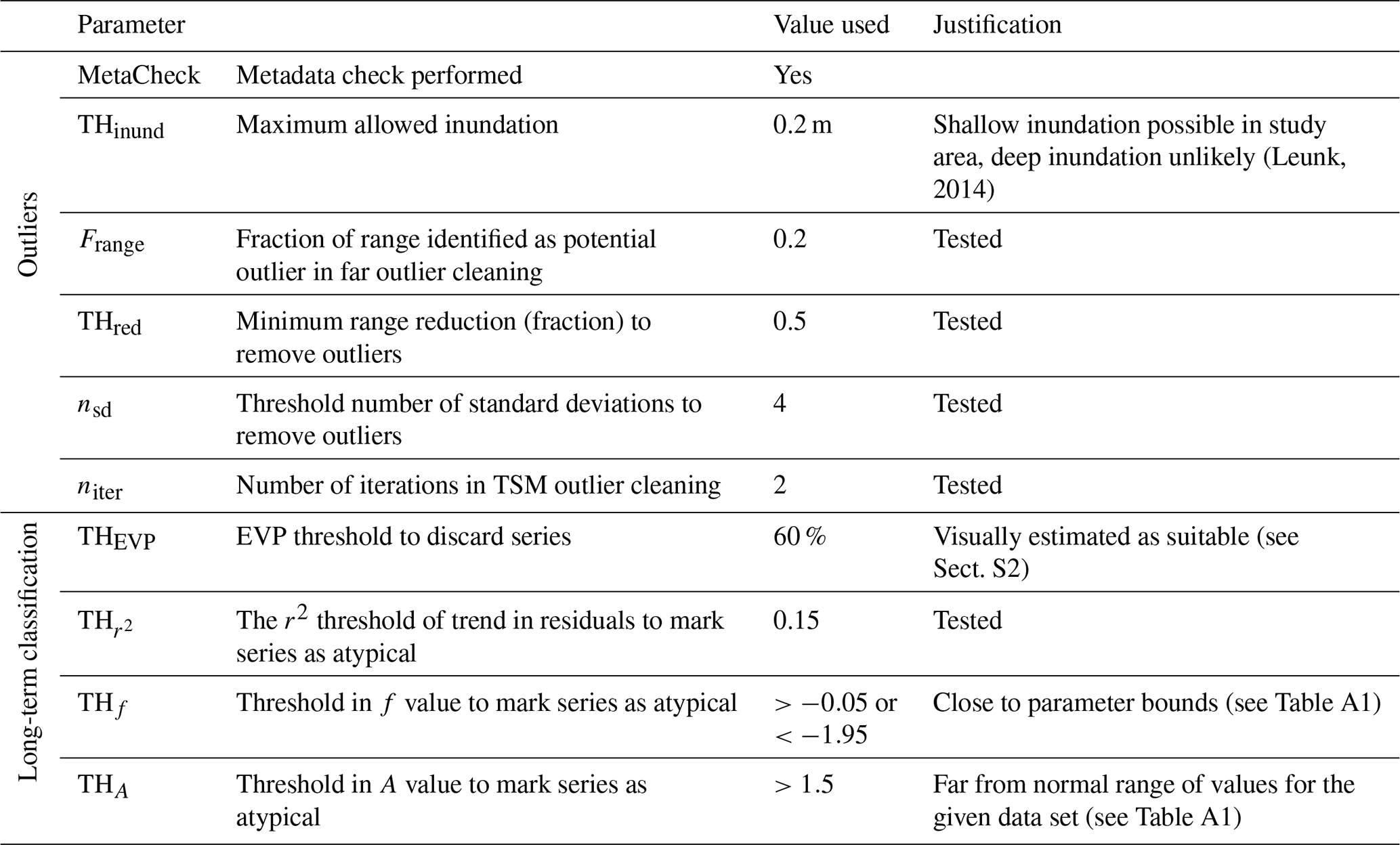
The outlier cleaning consisted of the following steps (see Table 1 for parameters):

1. Basic metadata consistency check. Measurements below the well filter or >TH_inund above the surface level were removed, as these are likely to point to erroneous measurements or metadata.

2. Removing far outliers by range. As a fast first cleaning step, far outliers were identified by isolating the top and bottom fraction of the measurement range (F_range) and identifying them as outliers if their removal caused a reduction in range of >TH_red.

3. Outlier removal by time series modelling. A model was fitted for each series using precipitation and ET_ref from the nearest weather stations. All measurements outside a range of n_sd times the standard deviation of the residuals around the simulation were removed. This step was repeated n_iter times to deal with outliers disturbing the model fitting (Peterson et al., 2018; Leunk, 2014).

For the long-term behaviour classification, a new time series model was fitted on the resulting cleaned series. The explained variance percentage (EVP, equal to r²⋅100) and model parameters A, f, and d were saved. In addition, a linear trend was fitted through the residual series, and the p value and r² of the trend were saved. Finally, the series were checked for consecutive periods with missing data of >4 years which would hamper the required 10-year data period (Sect. 2); if consecutive periods with missing data of >4 years were present, only the time period after the last data gap was used. Based on these indicators, the series were ordered into four categories of long-term behaviour (see Sect. S1 for examples):

1. Discarded series. These are series with very strong deviations from the expected behaviour (as indicated by EVP<TH_EVP) or insufficient data for analysis (<10 years, data gaps > 4 years, or no data over June–August 2018).

2. Deep-groundwater series. These are series with a mean water table depth (WTD) > 5 m that typically show a very slow, smoothed behaviour and often poor model fit; the used validation method is probably less suitable for these series.

3. Atypical series. These are series with mild deviations and EVP≥TH_EVP, but they contain a trend or atypical parameters. This points to potential errors, external (human) influence, or groundwater processes that deviate from the TSM assumptions used in this study. Locations were marked as atypical if they had a trend in the residuals with p<0.05 and $r^{\mathrm{2}}>{\mathrm{TH}}_{r^{\mathrm{2}}}$ or if they had unusual values for the f and A parameters (TH_f and TH_A).

4. Normal series. These are series with EVP≥TH_EVP and no other issues.

The cleaned measurement series of the normal, atypical, and deep categories were aggregated to daily means and saved for further use. Table 1 shows the validation parameters used for this study. Several parameters were chosen by initial trial-and-error testing; the sensitivity to these parameters was tested as explained in the following.

The performance of the validation method was evaluated on a test set of 180 randomly selected series (30 from each province). These series were visually checked for the occurrence of (1) outliers (series to clean); (2) serious long-term deviations, such as level shifts or strong trends (series to discard); and (3) milder long-term deviations, such as lighter trends (series to mark as atypical); see Figs. S1–S4 in the Supplement for examples.

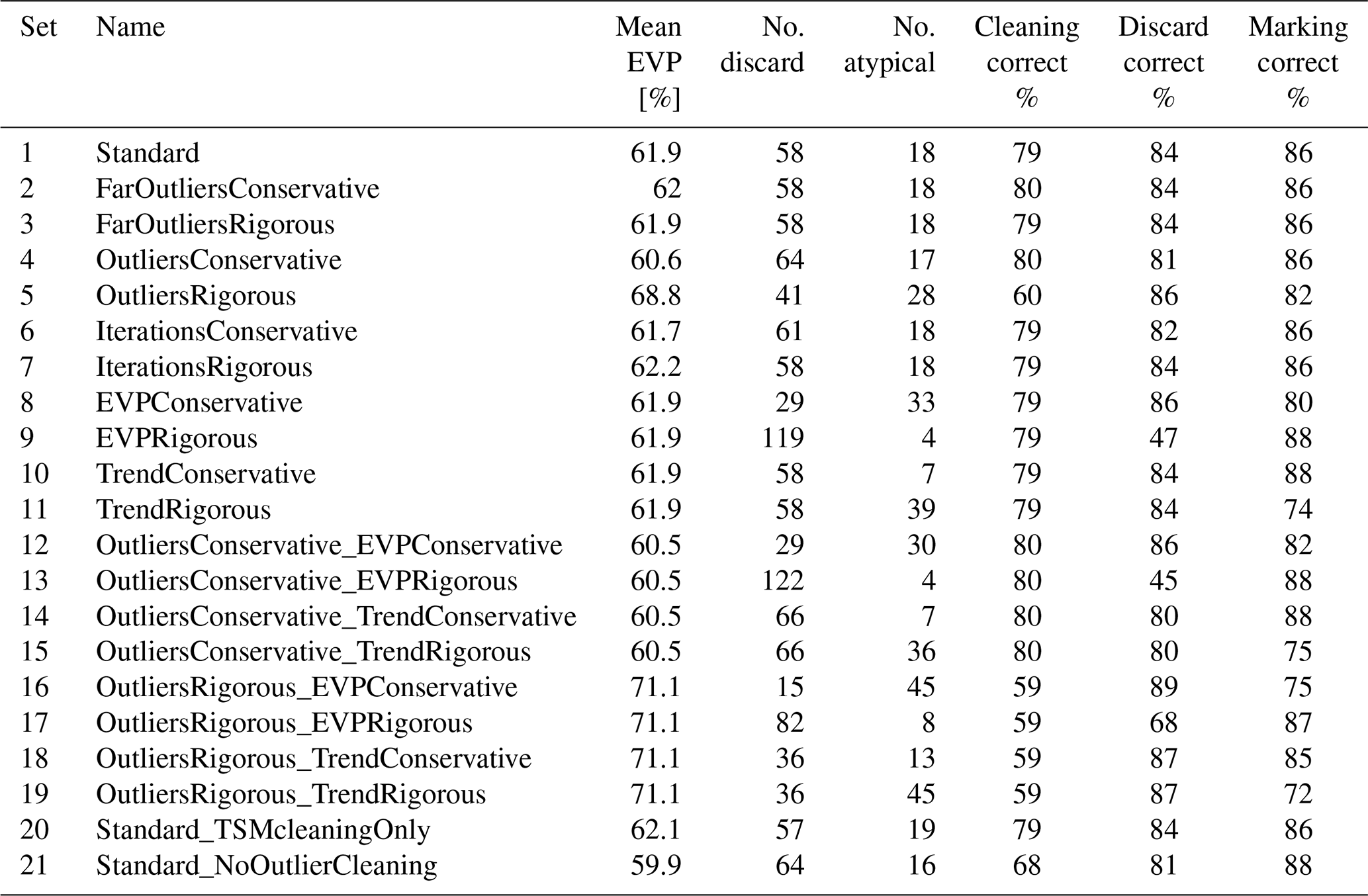
The validation routine was applied to the test set with the standard parameters shown in Table 1 and with 20 alternative parameter sets (Table S1 in the Supplement). In sets 2–11, the parameters were varied individually to more conservative (less cleaning and discarding) and more rigorous values (more cleaning and discarding); in sets 12–19, combinations of conservative and rigorous outlier cleaning as well as long-term deviation identification parameters were tested; and in sets 20 and 21, versions were tested with only TSM-based outlier cleaning (no basic cleaning step) and no outlier cleaning at all.

The validation results from all parameter sets were compared to the visual validation and scored by (1) correct identification of outliers (cleaned if needed), (2) correct identification of serious long-term deviations (discarded if needed), and (3) correct identification of mild long-term deviations (marked as atypical if needed). Scoring was done as true or false positive (deviations correctly recognised) and true or false negative (absence of deviations correctly recognised) for the three categories.

3.3 Series simulation

The cleaned series from the validation step were used to simulate groundwater heads for the drought analysis. It was chosen to use simulated series, rather than interpolating the measurement series with TSM (Marchant and Bloomfield, 2018), to ensure regular series without sudden level shifts and prevent influence of remaining outliers. A model was fitted on the cleaned measurement series (see Sect. 3.1 and Appendix A); for those models with an EVP >60 % (Table 1), a groundwater head series with a daily time step was simulated for the period of interest, in this case 1 January 1990 to 31 May 2020. As most measurement series originally ran until spring 2019, roughly 1 year of “nowcasting” was added to the data.

The performance of the simulations was assessed by the root-mean-square error (RMSE), the mean error (ME), and the rank correlation (Spearman's ρ) of the simulated groundwater levels (GWL) over the full length of the measurement series. ME was calculated as $\mathrm{ME}=\mathrm{mean}({\mathrm{GWL}}_{\mathrm{sim}}-{\mathrm{GWL}}_{\mathrm{obs}})$ to quantify bias. To assess model performance under dry conditions specifically, the measurements of each series were subdivided into “low-head periods” (measured head < 20th percentile), “medium-head periods” (20th to 80th percentile), and “high-head periods” (>80th percentile), and the RMSE and ME were recalculated for these periods. In addition, the RMSE and ME were determined specifically over July–November 2018, the period during which the meteorological and hydrological droughts peaked. The RMSE and ME were expressed both as the absolute value in metres and as a fraction of the mean water table depth at the location. The latter measure may give a better image of the scale of the errors, as the impact of a small change in groundwater head on vegetation and hydrological processes is generally much larger where groundwater levels are normally shallow (Bartholomeus et al., 2012; Witte et al., 2020b). Finally, average performance metrics were calculated for the three long-term behaviour categories (normal, atypical, and deep) separately.

The sensitivity of the simulation of drought conditions to the calibration period was also tested. Models were recalibrated on the period until the start of the 2018 growing season (1 April 2018), and the groundwater behaviour for the rest of 2018 was “nowcasted” with the available weather data. Simulation performance was again evaluated using the RMSE and ME over July–November 2018 and was compared with the simulations calibrated on the full period.

The groundwater behaviour at an individual measurement location can be summarised through the recharge response time, which can be derived from the fitted time series models. Here, the response time was defined as the time after which 50 % of the groundwater head response to a recharge event has occurred (e.g. Zaadnoordijk et al., 2019). It was derived by intersecting the step response function obtained from Pastas (function get_step_response) with the line 0.5 A. These response times are a characteristic of the full groundwater series, not just the drought period. Still, the response times and their spatial distribution give a further indication of the validity of the time series models and the drivers of groundwater drought development.

3.4 Drought index

To identify drought periods in time series of hydrological variables and to compare drought severity between locations, standardised drought indices are used. We quantified the development of meteorological drought over 2018–2020 using the standardised precipitation evaporation index, aggregated over 3 months (SPEI-3) (Vicente-Serrano et al., 2010). The study area was divided into four zones (see Fig. 2); the SPEI-3 for each zone was calculated from the average precipitation of all weather stations within the zone and the distance-weighted mean ET_ref of the three stations closest to the midpoint. This midpoint method was necessary to obtain representative values for each zone from the relatively few evapotranspiration stations present (15). The SPEI was calculated by a normal distribution transformation; the 3-month accumulation time was chosen because this most clearly showed the meteorological droughts at a timescale comparable to the variations in groundwater level.

For groundwater heads, the standardised groundwater index (SGI) was applied (Bloomfield and Marchant, 2013). The SGI method consists of transforming a measured groundwater head series at a specific location to a standard normal distribution; this produces a drought index series varying roughly between −3 and 3, indicating conditions from extremely dry to extremely wet compared with the normal situation. When analysing drought indices for multiple locations, a common reference period must be used. It is generally recommended to use a period of at least 30 years to ensure a proper estimation of the long-term “normal situation” (McKee et al., 1993; Van Loon et al., 2016; Ritzema et al., 2018). Here, the period from January 1990 to December 2019 is used throughout as the reference period.

For precipitation, the transformation step is usually done by fitting a gamma distribution function to the data (McKee et al., 1993). For groundwater heads, however, distribution shapes vary widely between locations (Bloomfield and Marchant, 2013; Dawley et al., 2019; Loáiciga, 2015). Fitting individual parametric distribution functions to each location based on the 30-year monthly series used here is likely to give unreliable results; for example, Link et al. (2020) found that more than 100 data points are needed for fitting reliable parametric distributions on hydrological series in most cases, while incorrect transformations give a high risk of biased drought index values (Svensson et al., 2017). Therefore, groundwater levels were transformed using a normal scores transform (see e.g. Bloomfield and Marchant, 2013). This is a non-parametric transformation method that has the advantage of being simple and transparent and also circumvents the risk of bias due to erroneous distribution fits. For each location, the simulated series was first aggregated to monthly mean levels. Transformation was then done separately for each calendar month. For each calendar month with n years of data, in this case 30, cumulative probability values are taken, uniformly spaced over the interval ($\mathrm{1}/\mathrm{2}n$) to ($\mathrm{1}-\mathrm{1}/\mathrm{2}n$); the corresponding SGI values are found by applying an inverse cumulative distribution function to these values. The resulting SGI values are assigned to the groundwater head measurements of the given calendar month by their rank from low to high. This method of calculating SGIs results in a limited number of “discrete” SGI values that correspond directly to the rank of the groundwater level compared to the rest of the reference period. Table 2 gives the SGI values and their corresponding rank and drought severity in this study. The drought severity classes follow the classification by McKee et al. (1993) that has been frequently used in drought studies. Note that the SGI, unlike the SPEI, is not aggregated over multiple months; therefore, the SGI values given here represent “SGI-1”.

Table 2 Categories used for the standardised groundwater index, with the corresponding groundwater level rank in a 30-year record.

The SGI values for the months outside the reference period (January–May 2020) were estimated by linearly interpolating the groundwater head–SGI relation for the calendar month. If the heads fell outside the range reached in the reference period, they were assigned the most extreme SGI value.

To test how the use of TSM simulations rather than measurement series affects drought analysis, SGI values were also calculated directly for a selection of locations that had long measurement series. To collect enough series for comparison while preventing the influence of differing time periods, a minimum of 27 years was used. All series with at least 27 years of data (starting before 1 January 1993) were selected from the cleaned measurement series, resulting in 531 series. The SGI values for 2018 were calculated in the same way as for the simulated series, with the SGI of a calendar month calculated only if at least 25 years of data were available. Thus, in some cases, the number of data points will be some smaller than for the simulation-based SGI. However, an n of 25 instead of 30 does not affect the classification for the lowest drought categories (as shown in Table 2); moreover, an exploratory test (not shown) indicated that the slight period mismatch did not affect the patterns in the resulting comparison. The simulation-based and measurement-based SGI values were compared by correlation (Spearman's ρ).

4 Results

4.1 Usefulness of the TSM method for drought data validation and simulation

4.1.1 Validation performance

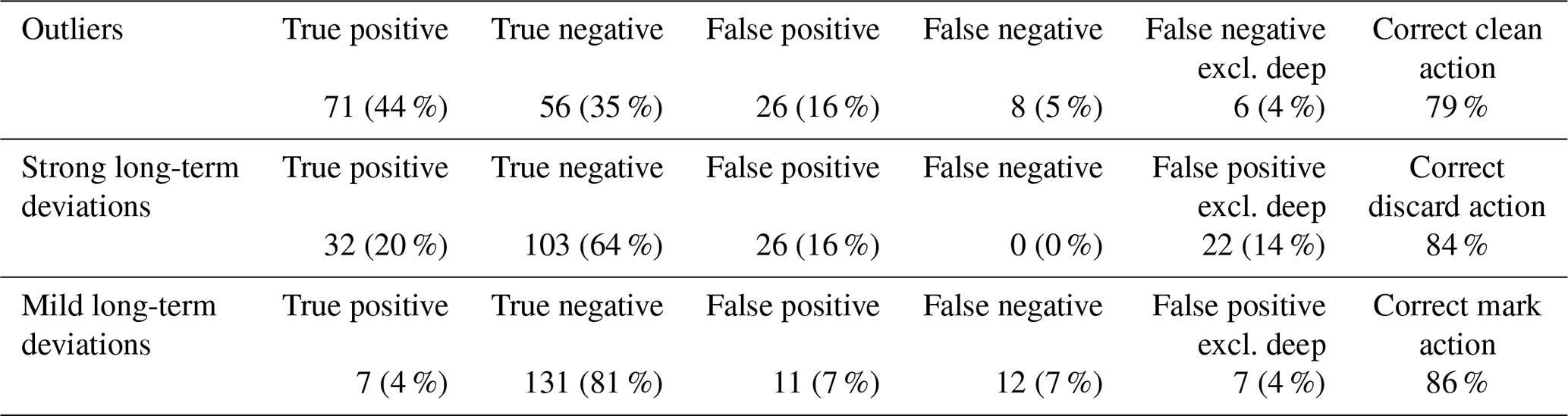
The validation performance for the standard validation parameter set is shown in Table 3. For a large majority of test series, the routine performed a correct action with regard to cleaning outliers, discarding strongly deviating series and marking atypical series. In the outlier cleaning, there is a relatively large fraction of false positives (removal of non-existing outliers). This mainly occurs for points in well-modelled series, without affecting the character of the series or the drought extremes. The false negatives (outliers not recognised) partly concerned influential outliers; another relatively frequent problem was the incomplete removal of a group of outliers (not shown in Table 3). With regard to the strong long-term deviations, there is a relatively large fraction of false positives (unduly discarded series). This is partly caused by the incomplete outlier cleaning for some of the series. The number of series marked as atypical by both the visual and automated validation is relatively small. This category is hard to identify consistently by visual inspection, which may explain the false positives and negatives.

Table 3 Validation performance for the standard parameter set (Table 1). The number of series with insufficient data is 19, so n_total=161. The terms used in the table are as follows: true positive – identified in both manual and automatic validation; true negative – not identified in either manual or automatic validation; false positive – identified in automatic validation but not in manual validation; false negative – identified in manual but not in automated validation; excl. deep – excluding deep-GWL series. The last column shows the percentage of series with outliers and long-term deviations correctly or reasonably identified.

The parameter sensitivity test (see Table 4 and Sect. S2) showed that the standard parameter set performed relatively well in comparison with other parameter sets. The sensitivity to the parameters of the far outlier cleaning (F_range, TH_red) and the number of iterations in the TSM outlier cleaning (n_iter) was low, while the standard deviation range for the TSM cleaning (n_SD) and the thresholds for discarding and marking series (TH_EVP and TH${}_{r^{\mathrm{2}}}$) did have a large effect. Applying an outlier cleaning step generally increased the simulation performance (mean EVP of 60 % to 62 %, set 1 vs. 21) and allowed more series to be retained for analysis (60 % to 64 % of series), with the TSM cleaning being responsible for most of the outlier cleaning. Taking a conservative low EVP threshold appears to give a good performance on the strong deviation identification (set 8 and 16), but the number of false negatives is high; in contrast, a strict EVP threshold of 80 % causes the majority of series to be discarded. Changing the threshold on the residual trend to mark series as atypical (set 10 and 11) caused either almost all or almost no series to be marked and did not substantially improve the performance.

Table 4 Summary results of validation parameter sensitivity test. No. discard and No. atypical refer to the number of series discarded or marked as atypical respectively. Cleaning correct %, discard correct %, and marking correct % refer to the percentage of series with correct action identified for cleaning, discarding, and marking respectively. See Table S1 for an explanation of the parameter sets.

When applied to the full study data set, the validation procedure discarded 31 % of the groundwater head measurement series, so that 1869 of the original 2722 series remained for analysis. A poor model fit was the most frequent cause for discarding measurement series. A total of 10 % of the series were maintained as atypical series, while another 12 % of locations had a deep groundwater table; these series were less suitable for the validation method used.

4.1.2 Simulation performance

In the simulation step, 1632 locations were modelled with sufficient quality (EVP > 60 %). Overall, these series were simulated with an average error of 14 cm, resulting on average in a 20 % error in the groundwater table depth (Table 5). The bias is low with a value of −1 mm. Subdivision into dry, normal, and wet conditions (0–20th, 20–80th, and 80–100th percentile of groundwater levels respectively) shows that the errors are larger for more extreme groundwater levels (dry and wet conditions). More precisely, the models tend to underestimate the extremes: there is a positive average bias in periods of low groundwater levels and a negative bias when groundwater levels are in their high ranges. Furthermore, during the main period of groundwater drought in July–November 2018, the simulation error is above average with a value of 18 cm. However, the ranking of the groundwater level is generally simulated well (mean Spearman's ρ 0.90), so that these absolute errors may not always propagate to the SGI values. Subdivision by the three quality types (bottom lines of Table 5) shows that the model performance decreases from normal to atypical to deep-groundwater series. For deep-groundwater locations, however, the errors lead to relatively small relative errors in WTD due to the large WTD at these sites.

Table 5 Performance of the groundwater head simulations for several subperiods and the three series types (Sect. 3.2). RMSE represents root-mean-square error, and ME is the mean error of simulations vs. measurements, given in metres and as fraction of the mean groundwater table depth (WTD).

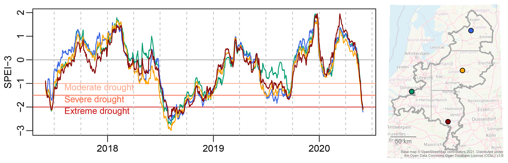
Figure 3 Development of the meteorological drought over 2018–2020 in the western, northern, central eastern, and south-eastern sections of the study area given by the 3-month SPEI. The map shows the four sections.

4.1.3 Calibration period sensitivity

In addition to the fully calibrated simulations, the sensitivity of the model simulations during drought to the calibration period used was tested (Table 5, last row of “Period”). When the 2018 drought summer was simulated with a TSM model calibrated until spring 2018, the average error in the predicted groundwater heads was 20 cm, giving a relative error in the groundwater depth of 31 % and, thus, performing slightly poorer than the fully calibrated simulations (error of 20 %). Similar to the fully calibrated simulations, there is a (small) negative mean error, indicating that the declines in groundwater level over summer and, thus, the severity of drought are slightly overestimated. This means that, as expected, the simulation of groundwater levels under extreme drought conditions outside the range of conditions in the model calibration has a relatively low reliability. However, the difference in average error is only 0.03 m, indicating that the effect is relatively small compared with the error already present in the fully calibrated simulations. There are no clear spatial patterns in the RMSE of the simulations (not shown). Thus, the sensitivity to the calibration period appears to be independent of specific catchment characteristics in the study area.

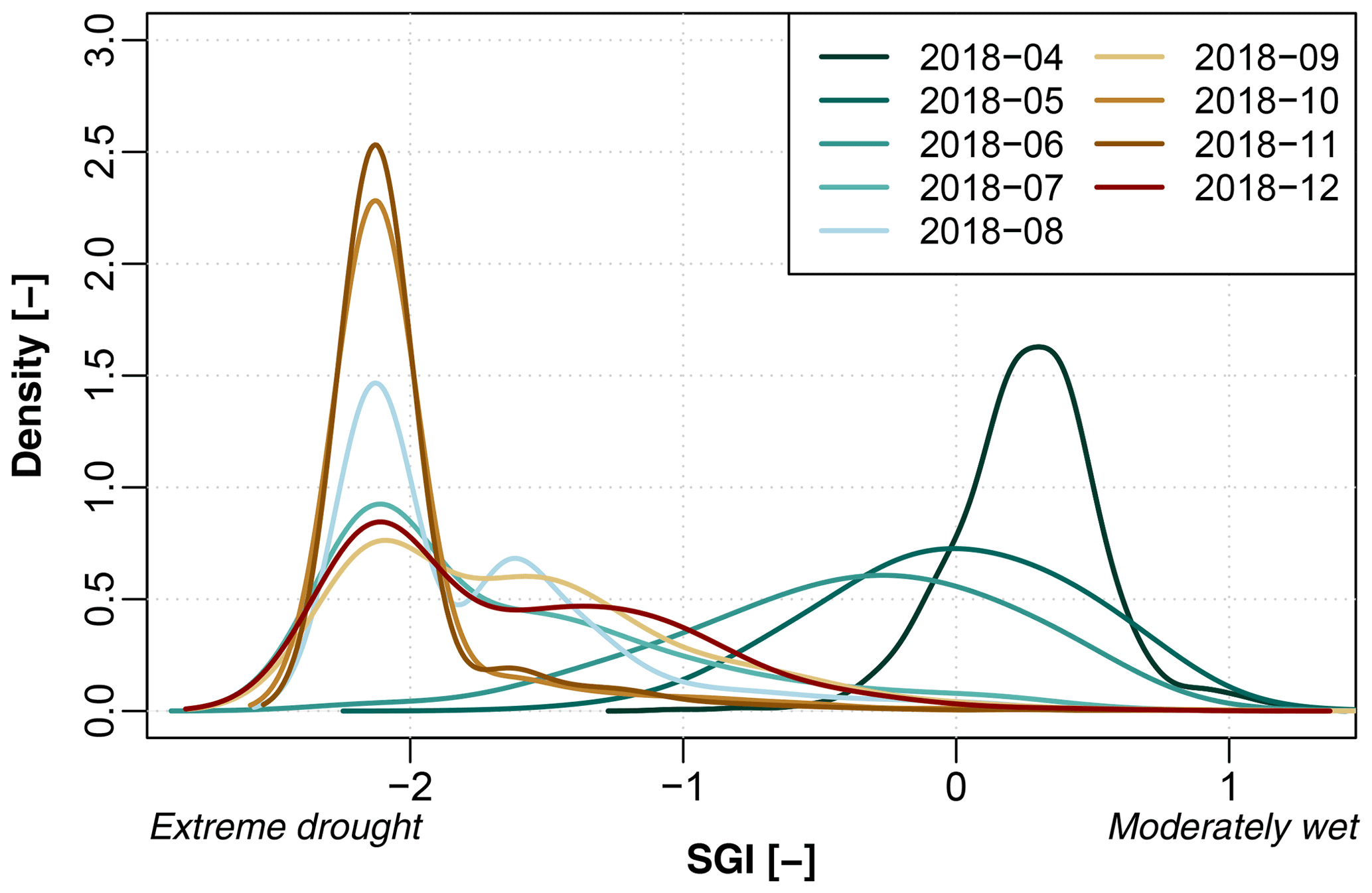
Figure 4 Monthly distributions of the standardised groundwater index over 2018 in the south-eastern Netherlands (months shown as yyyy-mm).

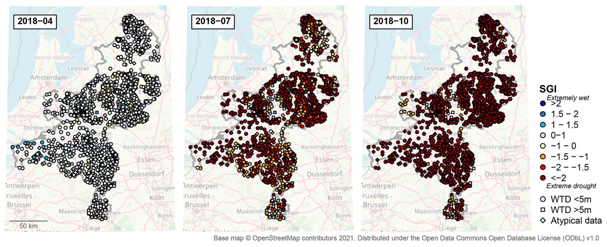
Figure 5 Groundwater drought development in 2018: SGI of simulated series in April, July, and October 2018. WTD denotes water table depth.

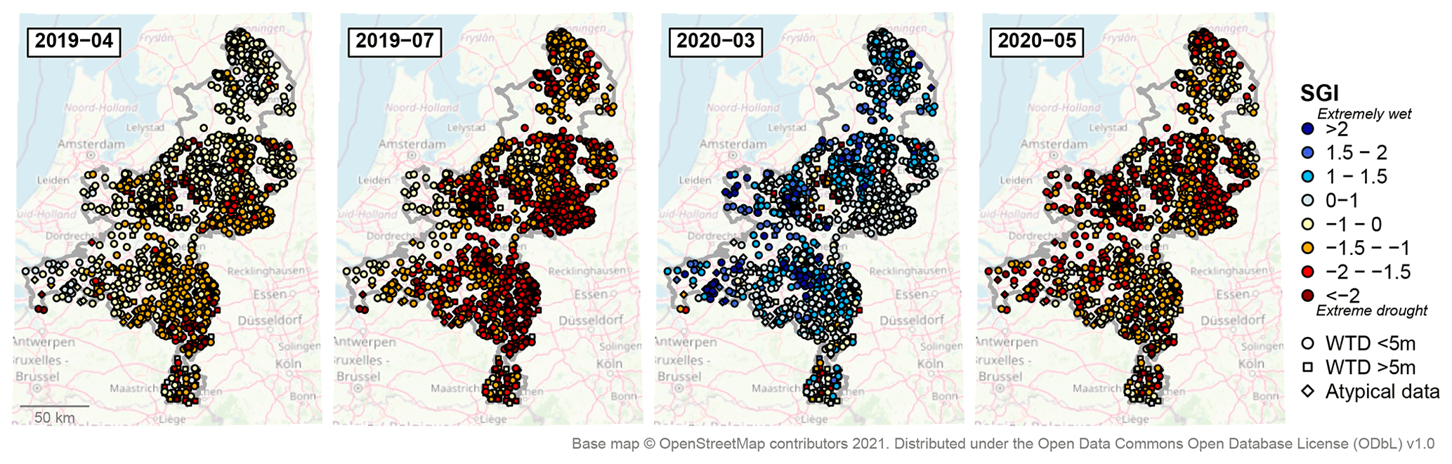
Figure 6 Groundwater drought over 2019–2020: SGI of extended groundwater series for April, July, March, and May 2019–2020. WTD denotes water table depth.

4.2 Development and recovery of the 2018–2019 groundwater drought in the Netherlands

The groundwater drought of 2018–2019 was driven by exceptionally dry weather conditions. The meteorological drought started in spring 2018 and peaked in late summer (Fig. 3). After a relatively normal winter, summer 2019 again showed moderate to severe drought. The winter of 2019–2020 was relatively wet, but exceptionally low rainfall in spring 2020 caused a return to extreme meteorological drought conditions. The meteorological drought was not spatially uniform. Especially in spring 2018 and summer 2019, the western part of the study area experienced less dry conditions than the east (Fig. 3).

The development of the groundwater drought in the south-eastern Netherlands over 2018 is visualised in Figs. 4 and 5. The 2018 growing season started with uniformly normal to high groundwater levels over the study area (Fig. 4). Drought started developing in May and June, with drought onset varying between locations. By July and August, severe to extreme groundwater drought occurred over most of the area. In September, heavy rain in the west of the study area slightly alleviated the drought conditions. However, the drought situation worsened again in autumn, reaching its height in October and November when the simulations show almost uniform extreme drought over the study area. By December, a slow recovery is visible.

The simulated data show distinct spatial patterns in the development of the groundwater drought (Fig. 5). Especially southern Limburg and the ridges in Utrecht and Gelderland with their distinct geology and topography (see Fig. 1) reacted more slowly than the rest of the study area and had not yet experienced drought conditions in 2018. Moreover, the fast recovery of the low-lying western Utrecht area in autumn stands out.

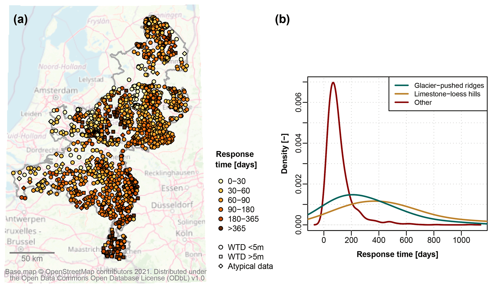
Figure 7 Response time to recharge as derived from the fitted response functions. See Fig. 1 for the location of subregions.

The simulations over 2019–2020 show that drought recovery was also strongly variable in space (Fig. 6). In spring 2019, groundwater heads in the west of the study area were again approaching normal levels, but the eastern regions had recovered poorly. By this time, extreme groundwater drought had also developed on the high ridges and in southern Limburg. The summer of 2019 again brought severe to extreme groundwater drought, this time clearly concentrated in the east of the study area, corresponding to the differences in meteorological drought. In March 2020, groundwater levels had returned to relatively high levels; however, the exceptionally dry weather in April rapidly resulted in a new severe drought situation by May.

The groundwater response times derived from the time series models are shown in Fig. 7. The response times are generally relatively short: 94 % of locations have a response time of less than 1 year. However, parts of the study area, especially the central ridges and the southern loess hills, show longer response times (Fig. 1). Thus, the spatial distribution of the response time corresponds with the topography and geology of the landscape. It also matches the patterns in the propagation speed of meteorological drought to groundwater drought in 2018–2020 (Figs. 5, 6).

4.3 Usefulness of the TSM method for regional drought assessment

For a subset of the locations (n=531), a long groundwater measurement series was available, and the SGI values resulting from the simulated series could be compared to those obtained directly from the cleaned measurement series (Fig. 8). The comparison shows that the simulations follow the same general drought behaviour as the measurement series, as the two follow a 1:1 line (Spearman's ρ=0.8). However, the simulations generally show a smaller spatial variation than the measurements. This is also visible in measurement-based SGI maps (Fig. 9), which show more scatter and local extremes than the simulation-based drought maps. In addition, the simulations for 2018 tend to slightly overestimate drought severity at the low ends of the drought (lower left in Fig. 8). This is contrary to the general tendency of the head simulations towards positive bias during drought periods (shown in Table 5).

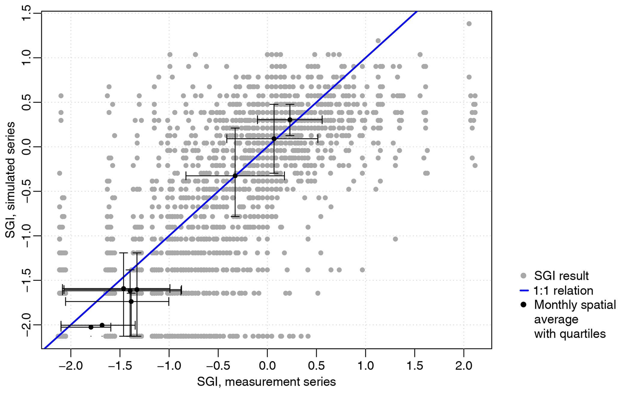
Figure 8 Comparison of SGI values over April–December 2018 based on cleaned long measurement series (x axis) and based on simulated series (y axis) for all location–month combinations (grey dots). Black dots show the average over all locations for each month, with quartiles (spatial variation).

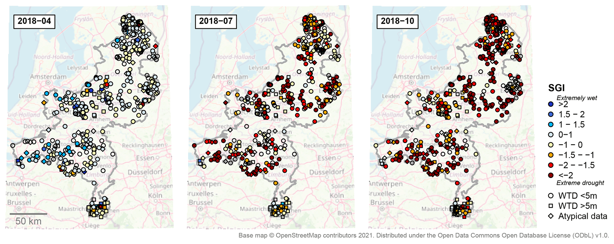
Figure 9 SGI for April, July, and October 2018 based directly on cleaned long measurement series. Empty symbols indicate insufficient data to enable drought index quantification.

5 Discussion

5.1 Usefulness of TSM data preparation for drought analysis

The performed study aimed to evaluate the usefulness of time series modelling-based data processing methods for groundwater drought studies. The application of a TSM-based method to the 2018–2019 drought in the Netherlands has provided new insights into how TSM methods can be used for data validation, how reliable they are for the quantification of extreme groundwater drought situations, and how they can contribute to regional groundwater drought assessments.

5.1.1 Validation methods for groundwater data

A validation method was applied that combines basic error tests with time series modelling-based identification of irregularities while also treating short-term outliers and long-term atypical behaviour separately. Pre-analysis outlier cleaning was found to improve the useability of series for the TSM simulations as well as the identification of long-term series' behaviour. Therefore, outlier cleaning is likely to improve results compared with performing a more limited validation or identifying impacted series only after simulation. The validation method performed reasonably with regard to outlier removal, although not optimally (Tables 3, S2). The time-series-based outlier cleaning appeared more effective in comparison with basic cleaning methods, although the latter can be valuable as a computationally cheap cleaning step for large data sets.

The TSM-based validation also appeared suitable for identifying long-term atypical behaviour in the head measurement series. However, the thresholds for separating series in different reliability classes (here “discard” and “atypical”) are likely to be dependent on the data used and the aim of the study, and they are difficult to set objectively. The current study aimed to provide a spatially detailed regional drought assessment, covering the range of site conditions; this requires retaining as many series as possible while also removing the most unreliable and disturbed series as well as identifying series with milder, potentially unreliable behaviour. The chosen parameters were found reasonable to reach this separation (see Figs. S5 and S6), but setting objective parameter values would require comparison with a large data set with detailed information on the sources of variations and errors, which was not available in this study.

In this study, we could not explicitly separate erroneous and real atypical patterns. Many of the long-term non-weather influences on the groundwater, such as structural abstractions and land use, are likely to be included implicitly in the simulations, as the time series models will model any external influence that correlates with weather or modifies the recharge response. Still, the validation is likely to retain some series with erroneous patterns and discard some real behaviour. The separation of errors could be improved by including additional driving factors in the time series modelling, such as surface water fluctuations (Bakker and Schaars, 2019; Van Loon et al., 2016; Zaadnoordijk et al., 2019); however, this requires substantially more data and modelling effort. Another potential approach is to make use of the spatial coherence of groundwater behaviour to separate errors. For example, Lehr and Lischeid (2020) and Marchant and Bloomfield (2018) used the spatial coherence of observed groundwater patterns as an indication of their reliability as well as to relate clusters of similar series to some external (human) impact. It would be valuable to explore such extensions of TSM to improve validation methods for groundwater drought analysis. This will allow for a better understanding of the different natural and human drivers of drought development.

Although the validation and simulation method generally performed well for the given data, it was less suitable for locations with deep groundwater tables (here >5 m), dominated by multi-year head fluctuations. Here, model fit was often low, leading to poor outlier identification and models being discarded for a large proportion of these locations (66 % discarded vs. 27 % for shallower locations). This issue was also found by Marchant and Bloomfield (2018) and Zaadnoordijk et al. (2019) for locations with thick unsaturated zones. To enable TSM simulation in such cases, measurement series are needed that are substantially longer than the minimum of 10 years used here in order to include several response cycles of the groundwater system.

5.1.2 Reliability of TSM groundwater level simulations during extreme drought

It was found that impulse-response function-based time series models on a general level produced reliable groundwater head simulations. They described most of the groundwater head series very closely, with a low overall bias (Table 5). The comparison of simulation- and measurement-based SGI values (Fig. 8) showed a good correlation (Spearman's ρ=0.8). Moreover, as discussed further below, the general patterns shown by the drought index maps match well with the experience of water managers during the 2018–2019 drought.

However, the model simulations also showed important deviations, especially at local scales and during the most severe drought periods. The simulation RMSE and mean errors amounted locally to high levels (Table 5), especially during more extreme conditions. Furthermore, relative errors, expressed as a fraction of the WTD, were often large (Table 5). This means that the application of the current TSM method could lead to misinterpretations of drought impacts at local scales, for example, on the survival of marsh vegetation or groundwater-dependent streams (Bartholomeus et al., 2012; Witte et al., 2020b). Generally, extreme conditions were underestimated somewhat by the time series models. This overall underestimation of extreme conditions was also found by Mackay et al. (2015) with a process-based groundwater model. Interestingly, the simulations for summer 2018 showed an overestimation of drought conditions, where the simulations appeared to miss the variability towards less-extreme drought that is visible in the measurements (Figs. 8, 9).

The model deviations during drought may be due to external influences not accounted for by the model, such as surface water influence and local irrigation, both of which are widespread in the study area. Indeed, local influences such as external water supply were found to alleviate groundwater drought locally in 2018 (Van den Eertwegh et al., 2019). In addition, the models may have underestimated the severity of earlier droughts; this would inflate the extremeness of the 2018 drought. Similar bias issues can be seen in Hellwig et al. (2020), who analysed groundwater drought in Germany using a physically based model. Their simulations overestimated drought severity during a drought in 1973, but not in 2003, confirming that bias can differ between individual drought events.

In addition, the deviations may be related to the model set-up itself. As noted before, we have worked with a simple linear recharge model here. Although this has been shown to suffice in many situations (e.g. Zaadnoordijk et al., 2019; von Asmuth et al., 2012), there are also various cases where linear recharge models were shown to be invalid (Bakker and Schaars, 2019; Collenteur et al., 2021). Non-linear or threshold responses in the soil–groundwater system may be especially important during extreme conditions, as evapotranspiration and deep percolation may become limited by low soil moisture or drainage may become disconnected (Bakker and Schaars, 2019; Aulenbach and Peters, 2018; Peterson and Western, 2014). Indeed, several studies have shown that non-linear recharge representations can improve model performance during (extreme) drought conditions (Berendrecht et al., 2006; Peterson and Western, 2014; Collenteur et al., 2021). The overestimation of drought severity in 2018 found here (Fig. 8) may, among other factors, be related to a lack of evapotranspiration limitation in the models (Collenteur et al., 2021). The effect of extreme drought on evapotranspiration and flow paths can be complex and spatially variable (Teuling et al., 2013; Avanzi et al., 2020). Therefore, further exploring the value of non-linear time series models for groundwater drought analyses in different situations is an important topic for future research.

The reliability of groundwater simulations during extreme drought was found to be sensitive to the calibration period used, with reliability decreasing when the calibration period lacked similarly extreme conditions. This is an important aspect for the application of TSM for groundwater level nowcasting for real-time drought assessment. However, the difference in simulation performance compared with simulations that did include the 2018 drought in their calibration was relatively small (Tables 5, 6). This suggests that the type of impulse-response time series models used in this study are relatively robust for series lengthening and nowcasting, even under drought conditions. This is also shown by the lengthened series over 2019–2020, which matched well with general observations provided by other studies and reports (LCW, 2020; Van den Eertwegh et al., 2019). Still, if water managers are to be provided structurally with up-to-date information on regional groundwater drought, any models have to be recalibrated frequently; hence, reliable, recent measurement data remain important.

Despite the potential loss of information caused by TSM-based data preparation, consisting of processes and external influences not included in the models, it also provides important gains. Given the spatial variability in hydrological drought dynamics and the need for long data series for drought identification, TSM methods can be especially useful in drought studies to increase the amount of data available without the need for additional site information. In this study, it enabled a regional image of drought development (Figs. 5, 6) that is far more detailed than that obtained by using direct measurement series only (Fig. 9). In addition, the model parameters gave additional insight in groundwater behaviour, for example, through the response time (Bakker and Schaars, 2019; Collenteur et al., 2019). Thus, TSM data preparation, especially if further developed, can likely be useful in many regional groundwater drought studies. However, in some cases, direct use of data, inclusion of more external drivers, or (a combination with) more physically based model methods will be more suitable (e.g. Bakker and Schaars, 2019), as may have been the case for more local scales in this study. Therefore, the application of TSM methods remains dependent on the aim and scale of a drought case study.

5.2 Analysis of the 2018–2019 groundwater drought in the Netherlands

5.2.1 Spatio-temporal development of groundwater drought in 2018–2019

The regional-scale analysis of the 2018–2019 groundwater drought in the south-eastern Netherlands provided a new, detailed image of the drought development in time and space. The analysis showed that extreme groundwater drought was widespread over the study region in 2018 and 2019, breaking 30-year records for the summer and autumn months almost everywhere (Fig. 4). However, the timing and duration of the drought varied strongly in space. In the western parts of the study area, drought was terminated before the end of 2018, whereas the higher-lying areas did not reach drought conditions until 2019 (Figs. 5, 6). This image corresponds well with how the drought was generally experienced by water managers. The Dutch commission on water allocation (LCW), which regularly surveys the drought status in the Netherlands based on input from water managers, reported widespread exceptional drops in groundwater levels, especially in the higher-lying sandy areas of the country, combined with a relatively fast recovery in the west (LCW, 2020). Moreover, the severe damage observed in groundwater-dependent ecosystems in the south-eastern Netherlands (Witte et al., 2020a) and widespread drying of groundwater-fed streams (Van den Eertwegh et al., 2019) match the assessment of an extreme groundwater situation.

The time series models made it possible to extend the available groundwater head measurement series beyond 2018 and obtain an estimate of drought recovery dynamics over 2019–2020. This showed that despite near-normal to high rainfall in the winters of 2018–2019 and 2019–2020 (Fig. 3), groundwater levels were restored only locally, and severe groundwater drought continued into 2019 or even 2020 over large parts of the study area (Fig. 6). These findings are consistent with general reports of the situation by local water managers (LCW, 2020; Van den Eertwegh et al., 2019). The results confirm that the drought should be viewed as a multi-year event rather than a single-year summer drought. The multi-year character increases the risk of lasting negative effects, especially in natural ecosystems. In addition, it stresses the importance of winter season groundwater management and water retention as determining factors in drought development. Both of these issues have already become apparent in the Netherlands after 2018 (De Lenne and Worm, 2020; Witte et al., 2020a, b).

5.2.2 Driving factors of spatial drought distribution

The current study did not aim to fully quantify the driving factors of the spatial variations in drought dynamics. However, the results suggest that the variation in drought severity, timing, and duration was governed mainly by the spatial distribution in rainfall and the landscape type. The influence of spatial variations in weather was visible in late 2018 and 2019. In this period, a gradient in meteorological drought towards the east caused groundwater drought to be concentrated in this area. The effect of the landscape type is visible for the higher-elevation parts of the study area, especially the glacial sand ridges and the limestone–loess hills, which clearly had a later, longer-lasting drought response than lower-lying areas (Figs. 5, 6). This pattern is also visible in the groundwater response times (Fig. 7). The slow drought response in the higher-elevation areas is likely explained by a thick unsaturated zone and low drainage density, whereas the fast recovery of the low-lying western parts may have been aided by thinner unsaturated zones and possibly some surface water influence. Other studies have found that these factors influence drought behaviour (Bloomfield et al., 2015; Hellwig et al., 2020; Peters et al., 2006; Van Loon and Laaha, 2015; Kumar et al., 2016). In addition, the elevation and geology in the study area correlate with variations in land use, soil type, and aquifer characteristics; these factors may have played an additional role.

The dominant role of landscape position in shaping drought development calls for locally adapted but also regionally coordinated mitigation strategies. The response times obtained from the time series analysis form a useful first indicator of the landscape characteristics that control the propagation of meteorological drought to groundwater drought. The response times found here are somewhat shorter than the drought response times reported by Van Loon et al. (2017) for part of the eastern Netherlands. However, they are very similar to those found by Zaadnoordijk et al. (2019), who performed time series analysis on groundwater series from the whole Netherlands. As they used different data and different model quality criteria, the similarity is reassuring and points to the stability of the time series models.

6 Conclusions

The performed study aimed to evaluate the usefulness of time series modelling-based data processing methods for regional-scale groundwater drought assessment. A TSM-based method was set up for data validation and drought quantification and applied to the regional 2018–2019 groundwater drought in the south-eastern Netherlands to test its usefulness and reliability. Automated TSM-based data validation was found to be able to improve the quality of input data. However, optimal validation parameters are likely to be context dependent. In addition, improvements in the validation method are desired, especially in the separation of real and erroneous head disturbances. The simulated groundwater head series were generally found to be reliable; however, it was shown that the use of time series simulations may bias drought estimations and underestimate spatial variability, producing large errors at a local scale. Still, the use of time series model simulations in drought analysis provides large advantages, as it enables a spatially detailed record of drought development that may be impossible to obtain with direct measurement series only.

The drought analysis for the south-eastern Netherlands provided a complete, detailed image of the development of the 2018–2019 groundwater drought in time and space. The findings confirm that the meteorological drought in 2018 caused extreme groundwater drought throughout the south-eastern Netherlands, starting in late spring and peaking in October–November of that year. The timing of drought onset and the duration of drought varied strongly in space. Drought development appeared to be governed dominantly by the spatial distribution of rainfall and the landscape type. In much of the area, the drought continued as a multi-year event into 2019 and 2020, especially in the eastern and higher-elevation regions.

Taken together, we conclude that time series modelling forms a useful tool to obtain a fast, detailed, and up-to-date image of drought development; however, for a proper understanding of the different driving factors of drought, the availability of recent and consistent monitoring data remains crucial.

Appendix A: Time series model set-up

Groundwater head modelling was done by impulse-response transfer function-noise models using the Pastas package in Python (Python 3.6, Collenteur et al., 2020). The model set-up used in this study largely follows Collenteur et al. (2019). The code for building and simulating the models, as applied in the validation and simulation steps in this study, is given in Fig. A1.

Figure A1 Python code used for building time series models with Pastas.

The working of impulse-response-type transfer function-noise models for groundwater series is explained in von Asmuth et al. (2002) and Collenteur et al. (2019). In principle, the method models groundwater heads as

$$\begin{array}{}\text{(A1)}& h\left(t\right)=\sum _{m=\mathrm{1}}^M{h}_m\left(t\right)+d+r\left(t\right),\end{array}$$

where h_m represents the variations in heads caused by one or several stresses m, d is the base level, and r is the residual at time t. Here, only recharge was used as an explanatory variable. Recharge is estimated as a linear combination of precipitation P and reference evapotranspiration ET_ref:

$$\begin{array}{}\text{(A2)}& R\left(t\right)=P\left(t\right)+f\cdot {\mathrm{ET}}_{\mathrm{ref}}\left(t\right),\end{array}$$

where f is a model parameter. The response of groundwater to a recharge impulse is calculated with a scaled gamma function (option ps.Gamma in Pastas):

$$\begin{array}{}\text{(A3)}& \mathit{\theta }\left(t\right)=A{\displaystyle \frac{t^{n-\mathrm{1}}}{a^n\mathrm{\Gamma }\left(n\right)}}{e}^{-t/a},\end{array}$$

where Γ is the Gamma function, A is a scale parameter, and a and n are shape parameters. The variation in groundwater heads over time h_m is obtained by convolution of this impulse-response function with the recharge time series.

Table A1 Parameter calibration settings: initial value and bounds during optimisation (default settings in Pastas); the range of values found in this study when modelling the initial 2723 cleaned series; and reliability bounds used for the series classification.

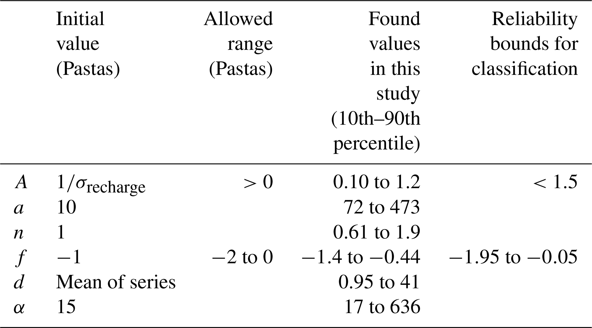
This gives five parameters to be fitted for each individual location. For purposes of parameter calibration, an autoregressive (AR-1) noise model is also fitted to the residuals, giving the additional noise decay parameter α. The default method for parameter optimisation was used, which minimises the sum of weighted squared noise by a least squares method (ps.LeastSquares). Table A1 gives the calibration settings for each of the parameters as well as the range found in the raw groundwater head series in this study. Based on these ranges, additional bounds were set for parameters A and f for the long-term behaviour classification (see Sect. 3.2); series with unusual parameters beyond these bounds were classified as “atypical” and potentially unreliable.

Except for the simulations used to test the calibration period effect, the full period of available data between 1990 and 2019 was used for calibration. Calibration was done at a weekly time step (recharge and observation series subsampled to a weekly frequency before optimisation) to allow for a more even spread of optimisation points over time. Simulation of series was done at a daily time step from 1 January 1990 to 31 May 2020.