Karst spring recession and classification: efficient, automated methods for both fast- and slow-flow components

Analysis of karst spring recession hydrographs is essential for determining hydraulic parameters, geometric characteristics, and transfer mechanisms that describe the dynamic nature of karst aquifer systems. The extraction and separation of different fast- and slow-flow components constituting a karst spring recession hydrograph typically involve manual and subjective procedures. This subjectivity introduces a bias that exists, while manual procedures can introduce errors into the derived parameters representing the system. To provide an alternative recession extraction procedure that is automated, fully objective, and easy to apply, we modified traditional streamflow extraction methods to identify components relevant for karst spring recession analysis. Mangin's karst-specific recession analysis model was fitted to individual extracted recession segments to determine matrix and conduit recession parameters. We introduced different parameter optimization approaches into Mangin's model to increase the degree of freedom, thereby allowing for more parameter interaction. The modified recession extraction and parameter optimization approaches were tested on three karst springs under different climate conditions. Our results showed that the modified extraction methods are capable of distinguishing different recession components and derived parameters that reasonably represent the analyzed karst systems. We recorded an average Kling–Gupta efficiency KGE > 0.85 among all recession events simulated by the recession parameters derived from all combinations of recession extraction methods and parameter optimization approaches. While there are variabilities among parameters estimated by different combinations of extraction methods, optimization approaches, and seasons, we found much higher variability among individual recession events. We provided suggestions to reduce the uncertainty among individual recession events and raised questions about how to improve confidence in the system's attributes derived from recession parameters.

1 Introduction

Groundwater from karst aquifers forms essential water sources globally (Stevanović, 2018; Goldscheider et al., 2020). Karst aquifers are characterized by a high degree of heterogeneity and complex flow dynamics resulting from the interplay of conduit and matrix drainage systems (Kiraly, 2003; Goldscheider and Drew, 2007). Groundwater flow is rapid in the highly conductive conduit system, whereas it is several orders of magnitude slower in the less conductive matrix system (Goldscheider, 2015). While both systems have significant storage capacities, the groundwater residence time is longer in the matrix than in the conduit system (Kovács et al., 2005). Several methods including detailed site-specific speleological investigation (Ford and Williams, 2007), tracer tests (Goldscheider and Drew, 2007; Goldscheider and Neukum, 2010), hydrograph analysis (Fiorillo, 2014; Kovács et al., 2005), and model ensembles (Fandel et al., 2021) are used to characterize groundwater flow dynamics in karst systems. Aside from hydrograph analysis, which usually requires only spring discharge time series data, other methods are either expensive to apply, time-consuming or require more input. This, therefore, makes time series analysis a commonly applied method for karst aquifer flow analysis and modeling (Ford and Williams, 2007).

Quantitative time series analysis provides lumped attributes of the karst aquifer system that are rather difficult to directly measure (Kovács et al., 2005). Karst spring recession analysis still remains a vital quantitative time series analysis tool for estimating aquifer parameters and geometric properties (Fiorillo, 2011). Discharge from karst springs reflects the complex interplay of conduit and matrix systems and provides insight into the characteristics of the aquifer which sustains the spring (Fiorillo, 2014; Kovács et al., 2005). This also provides essential information for flow prediction as the shape of the spring hydrograph reflects variable aquifer responses to different recharge pathways (Ford and Williams, 2007). Since the shape of the spring hydrograph describes in an integrated manner how different aquifer storages and processes control the spring flow (Jeannin and Sauter, 1998; WMO, 2008), analyzing individual recession limbs of spring hydrograph offers an extensive understanding of the structural, storage, and behavioral dynamics of the karst system's drainage (Bonacci, 1993).

Numerous studies have employed recession analyses of a karst spring hydrograph to characterize karst aquifers, evaluate aquifer properties, manage groundwater resources, predict low flow and estimate baseflow parameters (Padilla et al., 1994; Kovács et al., 2005; Fiorillo, 2014; Dewandel et al., 2003). Derived or estimated recession coefficients are also important parameters in karst models for simulating rainfall discharge (Mazzilli et al., 2019; Fleury et al., 2007) and other process-based modeling (Hartmann et al., 2013, 2014). Unlike porous media, karst systems cannot be represented by one single storage–discharge function (Ford and Williams, 2007). They comprise multiple subsystems of interconnected conduit and matrix reservoirs, each with its own storage–discharge characteristics (Jeannin and Sauter, 1998). Recession analysis models specifically developed for karst spring analysis are usually comprised of two (Mangin, 1975) or more (Fiorillo, 2011; Xu et al., 2018) independent storage–discharge transfer functions to describe drainage characteristics of different reservoirs and simulate recession flows. Dewandel et al. (2003) provide a general overview and main characteristics of commonly used recession models and those specifically applied to karst systems.

Even though recession analysis of spring hydrographs is cheaper in terms of resources required to explore the flow dynamics and geometry of the karst aquifer system, a major challenge in its application is the separation of the slow-flow (matrix-dominated) and quick-flow (conduit-dominated) components. The most commonly used karst spring hydrograph separation technique is the semi-logarithmic plot that usually reveals two or more segments. At least one of these segments, typically the last, represents linear reservoir drainage and is attributed to the slow-flow (matrix) component (Bonacci, 1993; Ford and Williams, 2007). The other segment represents the quick-flow (conduit) component – at times, a third segment representing the mixed component is also identified. However, this approach is visually supervised and subjectively applied, thereby resulting in imprecise and inconsistent estimations. The amount of time required for the visual supervision exercise also makes it impractical to apply this approach to a large number of hydrographs or multiple recession curves, especially if individual recession segment analysis is to be considered for parameter estimation.

However, in other fields of hydrology, there are a handful of automated recession extraction methods that have been developed for extracting streamflow recessions (Arciniega-Esparza et al., 2017). These traditional extraction methods aimed to explicitly identify baseflow recession periods by using different statistical indices to detect less variable flow conditions. During baseflow, streamflow is essentially supported by groundwater storage which provides a less variable flow condition. Contributions from runoff and other unregulated sources that produce highly variable flow during quick-flow recession are discarded by these extraction routines (Vogel and Kroll, 1996; Brutsaert, 2008). Although these methods were developed to extract baseflow recession from stream hydrographs, there is the possibility of adapting them for extracting matrix and conduit flow recessions of karst springs. In addition to identifying the slow-flow recession component, such adaptation will focus on recognizing the quick-flow component instead of discarding it. However, as these methods are based on different statistical indices for identifying the baseflow regime, they perform differently and produce differing recession parameters (Santos et al., 2019; Stoelzle et al., 2013). Therefore, while attempting to modify these routines, it is also important to explore and compare the differences in the estimated recession parameters that would result from adapting these commonly used traditional recession extraction methods.

Following the extraction of recession events, the estimation of recession parameters is done either by analyzing the individual recession segment (IRS) or constructing a master recession curve (MRC) from all events. The MRC approach is commonly used in karst hydrology studies to estimate spring recession parameters, though this approach is also considered to be very biased toward long recession events (Jachens et al., 2020). Also, the single parameters' value derived from this approach does not represent the actual dynamic nature and implicit heterogeneity of karst systems. However, parameters derived from IRS analysis better describe the range of the aquifer system dynamics as well as understanding the seasonal controls on recession behavior (WMO, 2008). While seasonal control on recession has been widely studied in porous media, studies assessing seasonal effects on karst spring recession are still rare. An advantage of the modified extraction methods presented in this study is that it allowed us to employ the IRS analysis for parameter estimation as well as project the analysis along seasonal dimensions.

Hence, this study aims to develop and test a robust and objective method for extracting karst spring recession components as well as determining the parameters associated with the different components of karst drainage systems. Therefore, in this study, we develop an automated karst recession extraction method that can identify matrix and conduit components of the karst spring recession hydrograph by modifying the traditional streamflow recession extraction routines. We then estimate conduit and matrix recession parameters of the IRS by using the combination of different modified recession extraction methods and parameter optimization approaches of the karst recession model. We explore the effect of seasonal influences on the karst conduit and matrix recession parameters as well as the aquifer system classification. Finally, the performances of the different combinations of modified extraction methods and karst recession model parameter optimization approaches were evaluated.

2 Data and methods

To develop an automatic karst-specific recession extraction and analysis procedure that is objective and applicable to large hydrograph samples, we first explored the applicability of traditional recession extraction procedures originally developed for non-karst streamflow recessions (Vogel and Kroll, 1992; Brutsaert, 2008; Aksoy and Wittenberg, 2011). Then we analyzed karst recession parameters using a two-reservoir parallel drainage recession model (Mangin, 1975). In the following subsections, the recession extraction and analysis model, parameter optimization approaches, as well as the various adaptations and modifications implemented are described. For consistency, we used the terms “quick flow” for the turbulent flow from highly conductive karst drainage pathways (synonymous with conduit and storm flow) and “slow flow” for the laminar flow contribution from less conductive fissures and pores (synonymous with matrix, diffuse, and base flow) (Atkinson, 1977; Larson and Mylroie, 2018).

2.1 Adapting streamflow methods to extract matrix and conduit recession components

Three streamflow recession extraction methods (Vogel and Kroll, 1992; Brutsaert, 2008; Aksoy and Wittenberg, 2011), herein called recession extraction methods (REMs), were adapted to extract matrix and conduit recession components (Table 1). To develop an automated baseflow recession extraction routine, Vogel and Kroll (1992) firstly smoothened the stream hydrograph using a 3 d moving average. Thereafter, the decreasing segments of the 3 d moving average are selected as the recession hydrographs. Only segments with 10 or more consecutive days are recognized as recession candidates. To exclude surface and storm runoff influence at the beginning of the recession, the first 30 % data points of each recession segment are deleted. Additionally, the difference between two consecutive streamflow values must be ≤30 % for the pairs to be accepted. All recession segments that satisfied these conditions are then accepted as slow-flow recession segments.

Table 1 Criteria for recession extraction methods (REMs).

To objectively determine a streamflow recession that is derived purely from a dry or low-flow period, Brutsaert (2008) introduced a stricter recession extraction method. For streamflow Q, during time t, the Brutsaert method eliminates data points with increasing or 0 values of $\mathrm{d}Q/\mathrm{d}t$ as well as points with abrupt $\mathrm{d}Q/\mathrm{d}t$ values. To exclude data points that might be influenced by storm runoff, three data points after a positive or 0 $\mathrm{d}Q/\mathrm{d}t$ are removed – in major events, an additional fourth data point is removed. While Brutsaert (2008) did not provide a description of a major event, Stoelzle et al. (2013) applied the Brutsaert method in their study and defined the major events as streamflow values exceeding 30 % frequency. Therefore, we used this definition of a major event from Stoelzle et al. (2013) in this study. Furthermore, the Brutsaert method also excludes the last two data points before a positive or 0 $\mathrm{d}Q/\mathrm{d}t$ and spurious data points with larger $-\mathrm{d}Q/\mathrm{d}t$ values.

Aksoy and Wittenberg (2011) extracted the baseflow component from the daily streamflow hydrograph during recession by comparing the coefficient of variation (CV) of the recession segment. All days with a decreasing or equal observed flow rate are considered part of the recession curve. Subsequently, a nonlinear reservoir model (Eq. 1) is iteratively fitted to the recession curve until the CV is ≤0.1. The CV is defined as the ratio of standard deviation between observed flow-rate measurements (Q) and calculated flow rate (Q_calc) to the mean of the observed flow rates as expressed by Eq. (2). A segment of the recession curve with CV ≤ 0.1 is selected as the real baseflow recession; otherwise, the segment is excluded. Only recession curves with 5 d periods or longer are considered. If the number of days becomes less than 5 during iterative curve fitting and CV ≤ 0.1 is not achieved, such a recession event is discarded (Aksoy and Wittenberg, 2011). To ensure consistency between the extraction method and the Mangin recession model used in this study (see Sect. 2.2), the value of b in Eq. (1) is set to 1, thereby making it a linear model.

$$\begin{array}{}\text{(1)}& {\displaystyle }& {\displaystyle }{Q}_t=Q_{\mathrm{0}}{\left[\mathrm{1}+{\displaystyle \frac{(\mathrm{1}-b)Q_{\mathrm{0}}^{\mathrm{1}-b}}{ab}}\right]}^{\frac{\mathrm{1}}{b-\mathrm{1}}}\text{(2)}& {\displaystyle }& {\displaystyle }\mathrm{CV}=\sqrt{{\displaystyle \frac{n^{\mathrm{2}}}{n-\mathrm{1}}}{\displaystyle \frac{\sum {\left(Q-Q_{\mathrm{calc}}\right)}^{\mathrm{2}}}{\sum (Q{)}^{\mathrm{2}}}}}\end{array}$$

The three recession extraction approaches (Vogel and Kroll, 1992; Brutsaert, 2008; Aksoy and Wittenberg, 2011) were specifically developed to extract streamflow recessions that are mainly from slow-flow contributions. The rules and exclusion criteria specified by each method are aimed at eliminating the quick-flow influences from the extracted recession segments. In karst systems, concentrated rapid flow through the conduit networks constitutes the quick flow, while the contribution from slow-velocity drains through the matrix pores constitutes the slow flow. The quick and slow flows represent flows from two different drainage structures, and both contribute to the karst spring recession (Fiorillo, 2014; Ford and Williams, 2007; Padilla et al., 1994).

Adapting the streamflow methods for karst spring recession analysis means considering both the slow- and quick-flow components to model matrix and conduit spring discharges. So, to adapt the traditional REMs, we (i) extracted the spring flow recession curve based on the specific method approach, (ii) attributed the part of the recession curve that satisfied the specified method's exclusion criteria as a slow-flow (matrix) component, and (iii) assigned the remaining part that is excluded as the quick-flow (conduit) component. Table 1 provides an overview of the rule-based baseflow recession extraction methods and changes made in adapting them to include the quick-flow component of recession.

2.2 Karst spring recession analysis

2.2.1 Mangin model

After extraction, we applied Mangin's (1975) recession analysis model which has been widely used for estimating drainage characteristics and aquifer dynamics in fractured non-homogeneous media (Schuler et al., 2020; Sivelle and Jourde, 2021; Fleury et al., 2007; Liu et al., 2010; Xu et al., 2018). To analyze the extracted recessions, we used this method which considers a two-component recession curve by distinguishing between quick-flow (mostly through karstic conduits) and slow-flow (mostly through the fissure matrix of the carbonate rock) recessions (Fig. 1). Mangin presented two equations: Eq. (3) describes the linear storage–discharge relationship from the saturated zone during slow-flow conditions represented by the Maillet (1905) equation.

$$\begin{array}{}\text{(3)}& {\mathit{\varphi }}_t=Q_{{\mathrm{r}}_{\mathrm{0}}}{e}^{-\mathit{\alpha }t},\end{array}$$

where $Q_{{\mathrm{r}}_{\mathrm{0}}}$ is the baseflow contribution at the beginning of recession when t=0, α is the recession coefficient with a unit of T⁻¹, t is the lapsed time between discharge at any time t, Q_t and initial discharge at t=0, Q₀, and Eq. (4) describes the nonlinear relationship during quick-flow recession from the unsaturated zone.

$$\begin{array}{}\text{(4)}& {\mathrm{\Psi }}_t=q_{\mathrm{0}}{\displaystyle \frac{\mathrm{1}-\mathit{\eta }t}{\mathrm{1}+\mathit{\epsilon }t}},\end{array}$$

where q₀ is the difference between Q₀ and $Q_{{\mathrm{r}}_{\mathrm{0}}}$, and parameter η describes the infiltration rate through the unsaturated zone. The parameter is defined as $\mathrm{1}/t_i$ for the duration of quick-flow recession between t=0 and $t_i=\mathrm{1}/\mathit{\eta }$. ε in T⁻¹ describes the regulating capacity of the unsaturated zone during infiltration and characterizes the importance of concavity of quick-flow recession (Padilla et al., 1994). The algebraic sum of Eqs. (3) and (4) gives Eq. (5), which defines the discharge at time t during the recession period.

$$\begin{array}{}\text{(5)}& Q_t={\mathit{\varphi }}_t+{\mathrm{\Psi }}_t\end{array}$$

Since t_i is the point of intersection of the slow-flow and quick-flow components of the recession curve and infiltration stopped when t>t_i ($t>\mathrm{1}/\mathit{\eta }$), the quick-flow component ψ_t in Eq. (5) is essentially assumed to be 0 at that point (ψt=0) (Civita and Civita, 2008; Ford and Williams, 2007). Therefore, the application of Mangin's model requires firstly fitting the slow-flow component ϕ_t to the slow-flow segment of the recession curve using Eq. (3) to determine the recession coefficient α. Afterward, Eq. (5) was fitted to determine the η and ε parameters of the quick-flow segment. However, the accuracies of $Q_{{\mathrm{r}}_{\mathrm{0}}}$, t_i, and the linear representativeness of the slow-flow component of the recession curve are critical for the reliable estimation of recession coefficients (Ford and Williams, 2007).

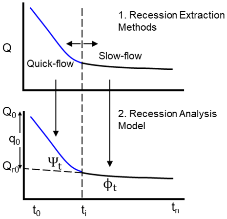
Figure 1 An illustration of the karst spring recession curve showing separation into linear and nonlinear components by the recession extraction method and fitting appropriate components of the recession analysis model.

2.2.2 Mangin classification framework

Following the estimation of recession parameters α, η, and ε using Eqs. (3)–(5) above, Mangin proposed a classification scheme for karst systems based on two additional parameters: (1) aquifer regulation capacity, K, and (2) infiltration delay, i. To determine K, the dynamic volume, V_dyn, which is defined as the volume of water stored in the phreatic zone at the peak discharge time t₀, is calculated using Eq. (6). The average volume of water, V_ann, discharged through the spring's outlet over 1 hydrological year is also calculated. The regulation capacity K is therefore given by the ratio of V_dyn and V_ann as expressed with Eq. (7). This parameter represents the extent of the phreatic zone and its ability to regulate groundwater release from storage. While porous aquifers can have values of K>0.5, a typical karst system is expected to have K<0.5 (Marsaud, 1996; Dubois et al., 2020).

$$\begin{array}{}\text{(6)}& {\displaystyle }& {\displaystyle }{V}_{\mathrm{dyn}}={\displaystyle \frac{Q_{{\mathrm{r}}_{\mathrm{0}}}}{\mathit{\alpha }}}\text{(7)}& {\displaystyle }& {\displaystyle }K={\displaystyle \frac{V_{\mathrm{dyn}}}{V_{\mathrm{ann}}}}\end{array}$$

The infiltration delay, i, represents the retardation between infiltration through the unsaturated zone and the spring's outlet. It is calculated as the value of the quick-flow component on the second day (t=2) of recession (Eq. 8). The value of i ranges between 0 and 1, where a system characterized by fast infiltration would have a value close to 0 and a slow infiltrating system tends towards 1.

$$\begin{array}{}\text{(8)}& i={\displaystyle \frac{\mathrm{1}-\mathit{\eta }\cdot \mathrm{2}}{\mathrm{1}+\mathit{\epsilon }\cdot \mathrm{2}}}\end{array}$$

With the parameters K and i, five classes of karst systems are defined (see also Fig. A1): (1) a well-developed system, (2) a well-developed speleological network with large downstream flood plains, (3) upstream karstification with retarded infiltration, (4) a complex system, and (5) a poorly developed system. Ford and Williams (2007) provided a detailed review of karst aquifer recession analysis and application of the Mangin model.

Table 2 Optimized recession parameters for the three different parameters of the optimization approaches (POAs) of the Mangin recession analysis model.

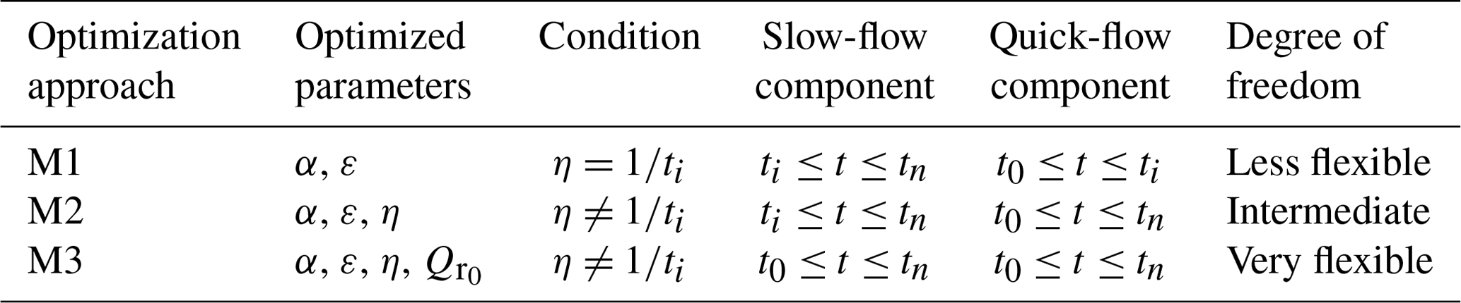
2.3 Estimation of recession parameters

For this study, the parameters were estimated for individual, automatically extracted recession events. That way, we captured the variability of spring discharge across individual recharge events (Jachens et al., 2020). To assess the effects of seasonal variation on the karst spring recession parameters, we separated the extracted events into summer and winter events. For simplicity, events that occurred between April and September of the hydrological year are considered summer events, while those from October to March are recognized as winter events. As mentioned in Sect. 2.2, in the standard Mangin approach, the slow-flow component of the recession curve (Eq. 3) is fitted at first to determine α. Also, the η parameter of the quick-flow component (Eq. 4), which is equivalent to $\mathrm{1}/t_i$, is predetermined, meaning that quick flow abruptly ends at t_i days, which cannot be considered optimal. Hence, reliable determination of t_i through the extraction routines (REMs) is vital for the estimation of the recession parameters. These standard procedures involved with the application of Mangin's model resulted in less degree of freedom for parameter interaction and an unrealistic abrupt ending of quick flow after t_i days. To increase the degree of freedom and assess the importance of t_i and the effect of a priori estimated $\mathit{\eta }(\mathrm{1}/t_i)$ on Mangin's recession model, we introduced three optimization approaches, which are referred to as parameter optimization approaches (POAs) in this study.

• M1: this follows the standard approach for applying the Mangin model as described by Padilla et al. (1994) and Ford and Williams (2007). The slow-flow component of the recession curve is fitted first with Eq. (3) for $t_i\le t\le t_n$ to determine the α value, while the quick-flow component is assumed to be 0 during this period. Afterwards, the second parameter ε is optimized by fitting the quick-flow component with Eq. (5) using the REM-predefined values of the η parameter ($\mathit{\eta }=\mathrm{1}/t_i$) for the event duration between $t_{\mathrm{0}}\le t<t_i$.

• M2: the conventional approach for fitting the Mangin model (M1) does not provide for an independent or flexible estimation of η. The prior definition of η as $\mathrm{1}/t_i$ relies on the accuracy of the extraction method to detect the point of inflexion t_i. This however does not give the flexibility to optimize η to a value that can provide a better fit for the model. To provide for a more flexible estimation of η, the α parameter is determined as in M1, and then Eq. (5) is fitted to the complete segment of the recession curve for $t_{\mathrm{0}}\le t\le t_n$ to determine the best values of the ε and η parameters.

• M3: this is a very flexible approach that allows for α, ε, η, and $Q_{{\mathrm{r}}_{\mathrm{0}}}$ values to be fitted numerically. The determination of t_i and $Q_{{\mathrm{r}}_{\mathrm{0}}}$ does not depend on the extraction method; rather, the best fit for the parameters is obtained from the optimization process. The Mangin model (Eq. 5) is fitted to the entire recession curve, which allowed for absolute flexibility of t_i and robust parameter interaction during optimization. With the model-calibrated $t_i(\mathrm{1}/\mathit{\eta })$, separating the quick- and slow-flow segments now entirely relies on the optimization exercise rather than extraction techniques.

For the optimization exercise, a nonlinear least squares procedure with spring discharge records was used. To avoid having a negative value of conduit drainage contribution when the optimized $t_i(\mathrm{1}/\mathit{\eta })$ is greater than the elapsing t value, the quick-flow component, ψ_t (Eq. 4), was constrained to a minimum value of 0. Table 2 provides a summary of the different optimization approaches, parameters that were optimized, as well as the duration of the optimized corresponding flow component.

2.4 Comparison and evaluation of REMs and POAs

The three REMs (Vogel, Brutsaert, and Aksoy) were combined with the three POAs (M1, M2, and M3) of the recession model to derive slow- and quick-flow recession parameters of selected karst springs for a total of nine possible methods. The recession parameters were derived separately for both summer and winter recession events. The overall performance of the different REM and POA combinations was determined by calculating the goodness of fit between observed spring recession discharges and ones simulated with the derived parameters using Kling–Gupta efficiency (KGE) measures (Gupta et al., 2009). We used KGE because it considers the common model error types – the mean error, variability, and dynamics. The mean and interquartile ranges of the derived parameters were compared among different method pairs and seasons. The estimated recession parameters were used to identify the dynamics of the systems according to Mangin's karst system classification described in Sect. 2.2.2. The Mangin classification scheme describes the aquifer drainage characteristics, conduit development, and speleological network (El-Hakim and Bakalowicz, 2007; Mangin, 1975). Therefore, this was used to evaluate the representativeness of recession parameters estimated for the selected karst spring aquifer systems.

3 Test springs and data

The REMs and POAs were tested using three karst springs, Lehnbachquellen, Saivu, and Qachquoch, located in Austria, Switzerland, and Lebanon, respectively (Fig. 2). The selection of these springs is based on the geographical spread, which covers different climate and hydrological settings, availability of the discharge hydrograph at high resolution, as well as literature references to the hydrological characterization of aquifer systems drained by the spring. Daily and sub-daily spring discharge time series of the selected springs were obtained from the WoKaS database (Olarinoye et al., 2020). Important characteristics of the spring hydrographs as well as the catchments in which they are located are presented in Table 3. The springs are located in catchments distinguished by different climate conditions according to the Köppen–Gieger classification (Beck et al., 2018). Lehnbachquellen is located in a snow-dominated, Saivu in a humid, and Qachquoch in a Mediterranean catchment. It should be noted that, in a snow catchment, recession behavior will be externally influenced by snow storage. However, we have included a snow-dominated catchment in this study to assess the impact of this external influence. The spring discharge time series was measured at a uniform time step for each spring and spanned between 3 and 13 years. All discharge time series were aggregated to daily temporal resolution, and missing data values which were only found (<0.01 %) in Lehnbachquellen spring discharge data were excluded.

Figure 2 Map showing locations of the three test springs obtained from the WoKaS database and different Köppen–Geiger hydroclimatic classes.

Table 3 Summary of test spring site properties and characteristics of spring discharge hydrographs.

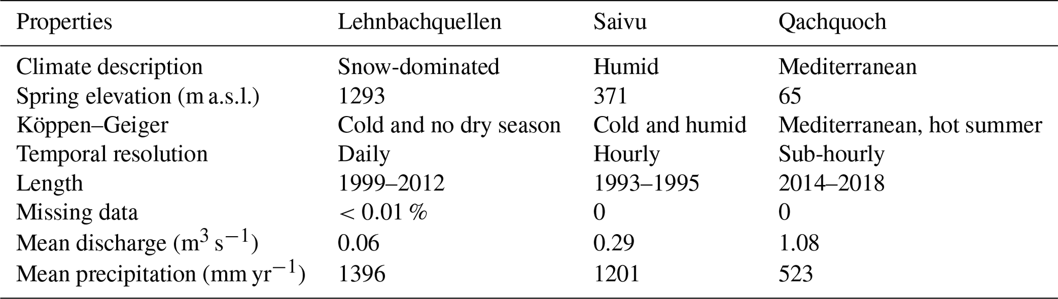
Table 4 Recession event period extracted by the REMs for the three spring discharge hydrographs.

4 Results

4.1 Extracted recessions and performances of POAs

The adapted recession extraction methods adequately identified karst spring conduit and matrix flow components. The parameters obtained with the different REM–POA pairs also produced satisfactory simulations of recession events. Only complete recession events ≥ 7 d were considered for analysis. Here, complete recession referred to events that featured both conduit and matrix components. For each spring hydrograph, a different number of recession events were identified by the REMs. As shown in Table 4, the Vogel method captured the highest number of recession events across all springs, followed by Brutsaert (except for Lehnbachquellen spring), with Aksoy showing the least ability to capture recession periods from the observed spring discharges. However, the average length of the recession events varied among the different REMs in no particular order (see Fig. A2). Based on the number of recognizable recession events, the REMs were defined as permissive (Vogel), less permissive (Brutsaert), and restrictive (Aksoy).

Figure 3 shows how the parameters derived from the different REM and POA combinations performed in simulating recession events using the KGE measures. With the exclusion of outliers, a high KGE value is achieved across all combinations, ranging between 0.70 and 1.0. More than half of all simulated events across the three springs produced a KGE > 0.9 for all REM–POA pairs. However, the lowest performance in all three springs is related to POAs combined with the Vogel extraction method. While there was no vivid observable pattern among the extraction methods (REMs) and recession model performances, the POAs showed otherwise. A clear systematic order for the KGE median is found within the POAs: M1 < M2 < M3. This is more noticeable in the humid and Mediterranean springs, except for the Vogel–M2 combination in the humid spring, which is not in the systematic order.

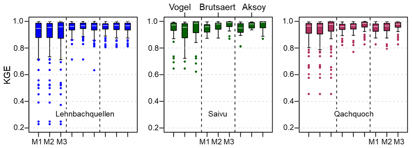
Figure 3 Boxplot of KGE measures between observed and simulated recession events based on parameters derived from the different REMs and POAs. The boxplots represent the interquartile ranges of KGE with the median shown in white lines and outliers marked in colored points.

4.2 Variability of recession parameters among the different REMs and POAs and seasons

Figures 4 and 5, respectively, show the results of the optimized slow-flow and quick-flow recession parameters for both the summer and winter periods. These parameter sets are combinations of α, η, and ε that produced the best simulation fit (i.e., the highest KGE value) with the different REM–POA pairs. Recession curve fitting based on the individual segment led to a large number of parameter combinations with the nine possible REM–POA pairs. The modification of REMs and POAs produced complex parameter interactions; for simplification, we explored the results along dimensions: (1) variability among the methods and (2) variability within seasons.

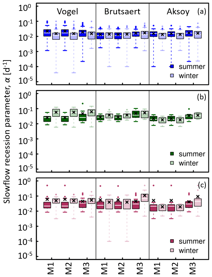
Figure 4 Distribution and variability of the slow-flow recession parameter, α, obtained by the combination of REM (Vogel, Brutsaert, and Aksoy) and POA (M1, M2, and M3) for summer and winter periods: (a) Lehnbachquellen spring in the snow-dominated catchment, (b) Saivu spring located in the humid catchment, and (c) Qachquoch spring in the Mediterranean catchment. The boxplots represent the interquartile range, whisker lines correspond to the most extreme parameter values, and outliers are marked as circles with corresponding box color.

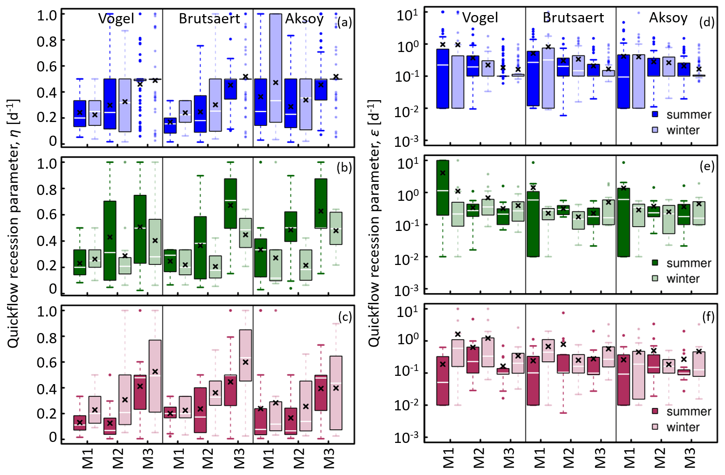
Figure 5 Distribution and variability of the quick-flow recession parameters, η and ε (y axis of ε in log scale), obtained by the combination of REM (Vogel, Brutsaert, and Aksoy) and POA (M1, M2, and M3) for summer and winter periods: (a, d) Lehnbachquellen spring in the snow-dominated catchment, (b, e) Saivu spring located in the humid catchment, and (c, f) Qachquoch spring in the Mediterranean catchment. The boxplots represent the interquartile range, whisker lines correspond to the most extreme parameter values, and outliers are marked as circles with corresponding box color.

The results from Fig. 4 show that REMs and POAs only have marginal effects on the estimation of the recession coefficient, α, when compared to the seasonality effect. Also, there are differences in how the REMs and POAs impacted the estimated values of α among the three karst spring catchments. Although the values of the mean, median, and interquartile ranges of α estimated by all the REMs for the snow-dominated catchment seem to be similar, slight differences can still be observed. The slow-flow recession parameters estimated by the permissive REM (Vogel) are within slightly higher ranges. On the other hand, the estimation of α in the humid and Mediterranean catchments seems to be more impacted by the POAs. By increasing the degree of freedom of the POAs, higher values of α are estimated, most noticeably with the M3 parameter optimization approach.

While the impacts of methodological approaches (i.e., REMs and POAs) are marginal on the estimated values of α, seasonal impacts on the values and variabilities of the parameter are more evident. The Saivu and Qachquoch springs in humid and Mediterranean catchments, respectively, showed similar dynamics in terms of seasonal variability of α, while the Lehnbachquellen spring located in a snow-dominated catchment showed a different seasonal dynamic. For the Lehnbachquellen spring, the values of the estimated α parameter are higher for summer recession events, noticeably with the Vogel and Aksoy extraction techniques (Fig. 4). During the summer period, estimated α values also showed less variability with the Vogel and Brutsaert REMs, while Aksoy gave more varied results for the same season. Meanwhile, an opposite situation is seen with the Saivu and Qachquoch springs. The median values and interquartile ranges of α are higher in winter for estimations done with the Vogel and Brutsaert extraction methods. For these springs, estimations associated with the Aksoy extraction method occasionally gave slightly lower α values during winter and less parameter variability. For all the spring systems, the seasonal variability of α is more observable with analysis associated with Vogel, which is the most permissive REM.

Both the recession analysis methodology (REMs and POAs) as well as seasons have significant impacts on the estimated values of the infiltration rate, η, and curve concavity, ε, parameters. The most visible pattern from Fig. 5 is that the increasing degree of freedom during optimization usually results in higher estimates (M3 > M2 > M1) and larger variability of η. However, this pattern may slightly vary among the different spring systems. The values of the η parameter spanned 1 order of magnitude for REM and POA combinations across all the spring locations. The springs in the snow-dominated (Lehnbachquellen) and Mediterranean (Qachquoch) catchments showed similar dynamics in terms of a seasonal variation of η. The estimated median and mean values of η are higher in winter for both springs. While parameter variability between seasons is relatively comparable in the snow-dominated catchment, larger variability is seen during winter in the Mediterranean catchment. In the humid catchment, the spring (Saivu) showed an opposite seasonal pattern, and summer events have higher η values as well as larger variability.

The estimation of the curve concavity parameter, ε, also reflected the influence of recession analysis methods and seasonal variations. The values of ε extend over 3 orders of magnitude across the three spring locations. In a differing pattern from η, increasing the flexibility of the POA led to low and more consistent ε values. We observed a decreasing order of M1 < M2 < M3 in the estimated values of the ε parameter for both the summer and winter periods, although combinations of Brutsaert and Aksoy REMs with the most flexible POA (M3) slightly contradicted this order at times, particularly for the humid and Mediterranean springs. Although the mean and median values showed slightly higher winter parameter estimations, the parameter ranges are similar for both summer and winter periods in the snow-dominated catchment. There is no consistent seasonal pattern in the dynamics of ε estimated for the humid and Mediterranean springs. However, an understated pattern is seen in higher (Saivu spring – humid) or lower (Qachquoch spring – Mediterranean) estimations of ε in summer, especially with the M1 parameterization approach.

In general, for the respective seasons, there is relatively better consistency among REM–POA pairs in estimating both slow- and quick-flow recession parameters, as shown by the results in Figs. 4 and 5. In fact, there is much higher parameter variability among recession events than the different REM–POA combinations and seasons.

4.3 Aquifer characterization

To evaluate the overall representativeness of estimated recession parameters based on the modified REMs and different POAs for the selected karst spring systems, we determined the drainage properties of the spring's aquifer using the parameters derived from the individual recession event. As described in Sect. 2.2.2, retardation between infiltration and output defined by the infiltration delay parameter, i, and aquifer regulation power, K, was calculated for individual recession events. Figure 6 shows the mean aquifer classifications as well as their standard deviations based on per-event estimated K and i values. The values of K and i were calculated for individual recession events with the recession parameters derived from the nine REM–POA combinations. As shown by the standard deviation bounds of the drainage properties derived from individual recession segments in Fig. 6, there is an overlap of calculated drainage properties and aquifer classes between the seasons. The methodological differences in the selected REM and POA resulted in large variations in the calculated mean values of infiltration delay, i, among the springs. The estimated mean values i for the three spring systems used in this study covered similar ranges (0.20 to 0.65). With the exception of the Lehnbachquellen spring, there was a good coherency in the mean K values determined from all combinations of REM and POA for each spring. In addition, the systems are more distinguishable by their ability to store and regulate groundwater outflow through the springs.

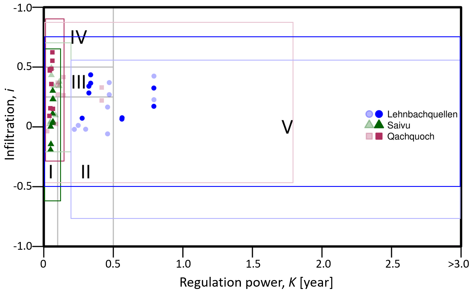
Figure 6 Karst aquifer type classification based on mean values of K and i calculated with recession parameters estimated by the different combinations of REM and POA for both summer (full-shaded color) and winter (light-shaded color) periods. Distributions of the per-event mean K and i derived from all method combinations for each spring are represented by colored symbols; areas covered by unfilled boxes are the standard deviations.

Among the three karst springs, only the Qachquoch spring showed a clear impact of seasonality in the system's classification. In summer, the estimated mean K values are <0.1 years, which is unanimous among the REM–POA combinations, whereas mean K values up to 0.45 and standard deviations of 1.75 years were estimated for the winter recessions. This resulted in a system classification extending from class I (well-developed system) to class IV (complex system) in summer and a system characterized as predominately class III (fairly karstified system) in winter. Groundwater has a very short residence time in the Saivu spring system for both the summer and winter periods. The mean regulation capacity of the system is <0.1 years, although a slightly higher value (ca. 0.15 years) was derived during the winter season. Due to this low regulation power, K, of the Saivu spring system, it was characterized predominately as class I in both the summer and winter periods. Only a handful of method combinations placed the system in class III.

While the other two springs (Qachquoch and Saivu) showed either clear or slight seasonal influence in the karst system characterization, the Lehnbachquellen spring did not show a systematic seasonal impact in its characterization. Both the estimated mean infiltration delay i and regulation power K showed a highly inconsistent pattern for the Lehnbachquellen spring. The mean K values ranged between 0.25 and 0.80 years, with standard deviation values > 3 years for both summer and winter recession events. With these high K values, the Lehnbachquellen system has the highest capacity to withhold groundwater among the three karst springs used in this study. The wide dispersion of both K and i made it impossible to confine the system to a specific class. The Lehnbachquellen system therefore falls within three classes: class II (a well-developed system with large downstream flood plains), class III, and class V (a poorly developed system).

5 Discussion

5.1 Quality of extracted recessions

With the modification of the traditional REMs, we were able to establish a completely objective approach to distinguish between slow- and quick-flow recession components. Furthermore, POAs with more flexibility showed better improvement over the conventional parametrization procedure. The REMs tested use different empirical approaches to scrutinize genuine baseflow records, and hence they have a different level of tolerance. The ability of the extraction methods to identify recession periods from hydrograph time series depends on the level of their restrictiveness. The Vogel extraction method defined by a 3 d moving average to smoothen the hydrograph and also allowing for a 30 % increase in subsequent flow rates is more permissive than the Brutsaert and Aksoy methods that strictly enforced $\mathrm{d}Q/\mathrm{d}t<\mathrm{0}$. Hence, more recession events were extracted by the Vogel method. A study by Stoelzle et al. (2013) also showed the Vogel procedure to be more permissive, as it was able to extract almost 50 % more events than Brutsaert. Although the main recession selection condition for the Brutsaert and Aksoy methods is determined by decreasing $\mathrm{d}Q/\mathrm{d}t$, constraining real baseflow recessions to discharge data points with less than 10 % (CV ≤ 0.1) deviations makes the Aksoy method more restrictive than the Brutsaert method.

Generally, all combinations of REM–POA performed acceptably well, and increasing restrictiveness of the extraction method gave an improved model performance. Even though restrictiveness led to better performance, this should not be a basis for outright accepting a restrictive REM over a less restrictive one. For instance, standard removal of 3 or 4 d by the Brutsaert method as a storm-flow-influenced period is speculative and could lead to an unrealistic estimation of conduit flow duration, t_i ($t_i=\mathrm{1}/\mathit{\eta }$), yet it performed better than the permissive Vogel method, although such a problem of unrealistic t_i estimation inherent in the Brutsaert method was eliminated, and general improvement in model performances was achieved by increasing parameter flexibility during optimization. Overall, the adapted REMs and the introduced three POAs provided a range of results that adequately represented the karst systems. However, there are still aspects of automated recession extraction that could benefit from further improvement for their general application in karst hydrology. For instance, the heterogeneous nature of the karst system results in a very dynamic spring discharge pattern; by introducing more tolerance to the REMs to accommodate the usual karst spring discharge anomaly, a longer recession event can be extracted. In addition, while all REM–POA pairs are good from the model performance perspective, it will be misleading to define the best pair of REM and POA based on this without evaluating whether the estimated parameters are realistic.

5.2 Effects of recession analysis methods and seasonality on extracted recession parameters

5.2.1 Effects of REM–POA combinations on extracted recession parameters

Methodological choices of REM and POA combinations have impacts on the estimated recession parameters. The extent to which the parameters are influenced by the methods largely varied between the slow- and quick-flow recession parameters. There was relatively higher consistency and better stability among all REM–POA pairs in estimating slow-flow recession parameters that describe the drainage characteristics of the matrix block within the phreatic zone. Depending on the catchment's hydroclimatic settings, both REMs and POAs proved to have marginal impacts on the estimation of the slow-flow recession parameters, though this is slightly contrary to other studies that found that slow-flow recession coefficients are majorly influenced by the extraction method used, while the parameterization approach only has a marginal impact (e.g., Stoelzle et al., 2013; Santos et al., 2019).

Although the combination of REM and POA affected the estimation of conduit drainage characteristics, the effect of the POA is more pronounced. Increasing the degree of parameter freedom during optimization with the different POA formulations often resulted in a significant reduction in the variability of the parameters. This was also accompanied by either low or high estimation of conduit drainage parameters. The more flexible parameterization approaches (M2 and M3) generally led to higher infiltration rates through the unsaturated zone. The infiltration rate is predetermined ($\mathit{\eta }=\mathrm{1}/t_i$) in the original parameterization procedure of Mangin's model (M1), thereby restricting the fitting of the quick-flow recession curve only to the optimization of parameter ε, which regulates infiltration through the unsaturated zone. The values of ε smaller than 0.01 have been reported as indicating very slow infiltration, and values between 1 and 10 show a domination of fast infiltration (Ford and Williams, 2007; El-Hakim and Bakalowicz, 2007). To compensate for the inflexibility due to the predetermined infiltration rate, the regulation effect of the unsaturated zone was amplified, which is evident in the higher and more varied values of ε estimated with the M1 parameterization procedure. By means of excluding a fixed number of days (3–4) as the influenced stage of recession, Brutsaert paired with M1 also led to similar values of η estimated for all springs. This makes it an unsuitable combination, especially with a long recession period. In their study, Santos et al. (2019) found analysis with the Brutsaert method to be more robust and appropriate for short recession samples.

Despite the impacts of methodological choices on the uncertainty of estimated recession parameters, variability among events exceeded the variability among methods. These high variabilities are attributed to different lengths of extracted recession events, differences in karstic processes such as recharge, infiltration, as well as conduit pathways that are activated within the unsaturated and saturated zones for each event. Even though karst systems are very heterogeneous and it is important to capture the impacts of the variable karstic processes through the analysis of individual recession segments, the high uncertainty among events makes it difficult to define a set of representative recession parameters.

Per-event recession analysis is very useful for better understanding the karst system dynamics compared to master recession analysis, which is unable to depict the hydrodynamic behavior of karst. However, the high uncertainty found with this approach is still a challenge and a bit difficult to cope with. We believe there are still possibilities for improvement with this approach; for example, defining a systematic approach to quantify parameter uncertainties will help to increase the confidence of the individual recession segment analysis.

5.2.2 Seasonal influences on recession parameters

The seasonal variability of the slow-flow recession parameter is interconnected with the choice of REM. Among the three different REMs used in this study, a clear seasonal variability of α was more noticeable with Vogel, which is the most permissive REM. However, the observed seasonal variability diminished with increasing restrictiveness of the REM. Also, the pattern of the seasonal variability of α was not the same for all three catchments, and this emphasized the influence of climatic controls on karst aquifer drainage. For instance, humid and dry regions are usually characterized by long recession and perhaps a significant drop in the groundwater table during summer. From the results presented in the previous section, we identified lower values of α in summer compared to winter. As the parameter α signifies the slope of slow-flow recession, a higher value means a steeper slope and faster emptying of the aquifer. The lower α values seen during summer emphasized the drought resistance of the system due to a decrease in the aquifer hydraulic head. Meanwhile, the snow-dominated catchment showed an opposite behavior, with higher values of α in summer. This occurred due to the accumulation and melting of snow. The snow melting process during the summer period would result in a higher hydraulic head, while frozen ice packs in winter translate to a lesser hydraulic gradient. As previously mentioned, a higher hydraulic head would promote faster drainage of the aquifer, resulting in higher values of the α parameter.

For quick-flow recession parameters, seasonal variability is independent of the REM. The three springs showed different seasonal patterns which could be directly linked to their hydroclimatic settings. Seasonal influence on quick-flow recession parameters was not clearly seen in the snow-dominated catchment. This could be attributed to the snow melting process discussed above. Since snowmelt compensates for hydrologic flow during warmer periods, there would be a constant influx from the surface throughout the year, and soil wetness conditions would not change significantly. This explains the lack of any evident seasonal differences between parameters η and ε estimated for the Lehnbachquellen spring in the snow-dominated catchment. However, the Saivu spring in the humid and Qachquoch spring in the Mediterranean catchment showed clear seasonal influences. Estimated values of infiltration rates η for Saivu were higher in summer (lower in winter) and lower in summer (higher in winter) for the Qachquoch spring. This pattern is believed to be controlled by the peculiarity of the different geographic and climatic settings. In a humid catchment, higher temperatures in summer would result in drier soil conditions, which would consequently facilitate faster infiltration. However, for the Mediterranean settings, soil conditions are dry due to relatively warmer temperatures all year round. This makes precipitation a limiting factor, and with more precipitation in winter, faster infiltration through the unsaturated zone would occur.

5.3 How realistic are adapted REMs and POAs for karst system analysis?

The karst system classification proposed by Mangin (1975) is based on two parameters, K and i (see Sect. 2.2.2). These two parameters were derived from the estimated recession parameters (α, η, and ε), and thus the variability found in the recession parameters is expected to be propagated to K and i, although, if the derived mean values of K were considered, some level of coherency was found among all REM–POA combinations and between the seasons. However, looking at the estimated standard deviations, a large intra-event and seasonal variation can be found. In a study by Grasso and Jeannin (1994), the authors found regulation power, K, to be more stable for various years and events. These findings did not agree with our analysis, the outcomes of which showed a large variability among K for different events, most significantly in the snow-dominated catchment. Regulation power is analogous to the memory effect, and the periodic water release from external snow storage that is not captured within the saturated zone in real time makes K fluctuate more in the snow-dominated catchment. Considering the standard deviations from the mean, in fact, the values of K exceeded the maximum value of 1 originally proposed in the Mangin karst classification scheme. Mangin (1975) set a maximum value of 1 for K, with assumptions that real karst systems would not have a storage memory beyond 1 year. However, a karst system in a snow catchment could have K values greater than 1 due to snow accumulation and melting as found in the Lehnbachquellen spring. Also, complex aquifer systems, as in the case of the Qachquoch spring, could also have higher K values.

Infiltration delay, i, is strongly dependent on recharge-type contribution as well as catchment size (Jeannin and Sauter, 1998). Recharge is controlled by climatic input (rainfall) which varies between seasons. However, the derived values of i were hardly separated by season but were more varied among individual recession events. The complex interplay of REM and POA resulted in a compensation phenomenon whereby the infiltration rate, η, was compensated by the recession concavity parameter, ε. Since the infiltration delay is defined by these parameters, it is difficult to explicitly infer the specific effects of REM and POA on infiltration delay.

The northern Alps karst system where the Lehnbachquellen spring is located has been defined as a well-karstified highly permeable unit interlayered with less permeable flysch formation (Chen et al., 2018; Goldscheider, 2005). Our analysis partly placed the karst system in classes II and III, thereby showing some consistency with literature evidence. Perrin et al. (2003) described the Saivu spring system as a well-developed karstic network, and the majority of the method pairs used in this study placed this spring in class I, therefore coherently agreeing with the authors' description. Taking into account the standard deviations, the classification of the Qachquoch spring ranged between a medium and poorly karstified system. This is similar to a recent study by Dubois et al. (2020) that categorized the system as poorly karstified with a very large regulation capacity.

Given that the existing common karst spring recession extraction method involves a visually supervised procedure and subjectively determined duration of conduit infiltration, an alternative faster, automated, and objective approach is very useful. From our analysis, the resulting parameters of extracted recession segments are within reasonable ranges, and the derived systems' classifications correspond to those found in the literature. The good performance recorded between simulated and observed flow rates during recession events attests to the potential transferability of traditional extraction methods to karst systems. However, this good performance does not necessarily translate to reliable parameter estimates. It is therefore important to choose REM methods that give reasonable parameters, especially when paired with a less flexible optimization approach. Furthermore, with prior knowledge of the spring system, parameters ranges can be reasonably constrained during optimization to achieve more representative optimum parameters.

6 Conclusions

The application of karst spring hydrograph recession analysis is very broad, including estimation of storage capacity (Fleury et al., 2007), describing discharge of the unsaturated zone (Amit et al., 2002; Mudarra and Andreo, 2011), as well as system classification (El-Hakim and Bakalowicz, 2007). Most often manual recession extraction is used, and the high subjectivity of the approach introduced bias to estimated parameters. For the first time in the literature, this study explored the applicability of automated traditional recession extraction methods (REMs) originally developed for slow-flow (baseflow) recession by adapting them to also identify quick-flow recessions. We fitted individual extracted recession segments with Mangin's recession model to determine the conduit and matrix drainage recession characteristics. We introduce new parameter optimization approaches (POAs) different from the conventional procedure to increase the degree of freedom of parameter interaction.

While we found that there were uncertainties in the estimated recession parameters resulting from the methodological choices (REM and POA combinations) and seasonal influences, the uncertainties among individual recession events were much larger. The large variability among individual events actually reflected the dynamic heterogeneous nature of the karst system. The combination of this with REMs, POAs, and seasons resulted in a more complex interplay and only amplified the uncertainties. These uncertainties are actually useful for understanding the dynamic nature of the karst system, but it is difficult to cope with and also needs to be systematically quantified. To avoid these large uncertainties, a master recession analysis approach has been a popular alternative for karst spring hydrograph analysis. However, a single recession parameter's values derivable from the master recession approach do not reflect the highly dynamic nature of the karst system. The uncertainty of karst recession parameters derived from either the single or master recession approach is presently not a discussion in karst hydrology. Maybe such discussion needs to start to address the limitations and difficulties encountered in this study. Herein, we pose two major issues that need to be addressed as seen in this study: (1) how can we do recession analysis more objectively with a single REM and separation technique that accounts for all ranges and possible instances of slow and quick flow, and (2) how can we incorporate a more robust parameter estimation and uncertainty quantification approach into individual recession analyses? Answering these questions will help to expand confidence in the system's drainage characteristics that are derived from recession parameters.

Finally, this study has shown that there is a lot of potential for extracting and separating karst spring recession components by adapting the traditional REMs and introducing flexible parameter optimization approaches. The adaptation of the REMs in combination with the different parameter estimation flexibility (POAs) provides a suite of automated tools that can be used for karst recession study. This automated multi-approach for parameter optimization is essential for coping with the known biases of single and visually supervised recession analysis methods. Different REMs have their specific advantages, and there is still room for improvement. For example, other extraction methods can be tested and nonlinear reservoir models can also be considered for fitting the matrix model.

Appendix A

Figure A1 The Mangin (1975) karst system classification scheme based on K and i.

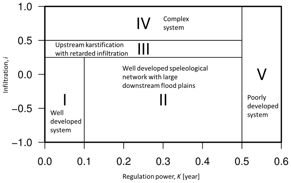
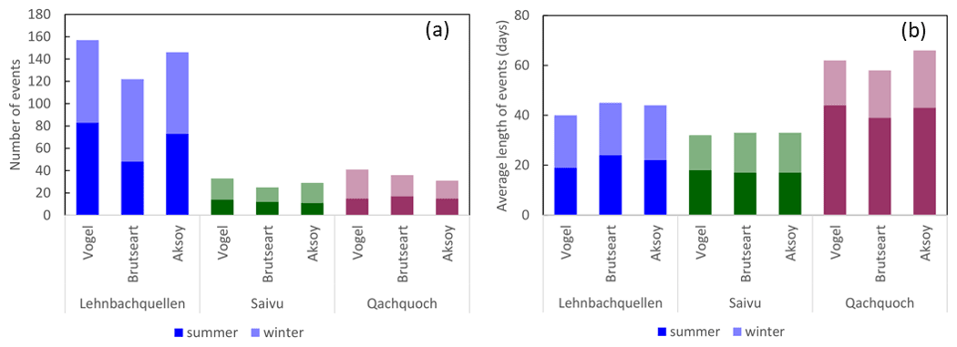
Figure A2 Characteristics of extracted recession events by REMs for both winter and summer periods at the three study sites: (a) number of identified complete recession events and (b) the average number of days when complete recession occurred.

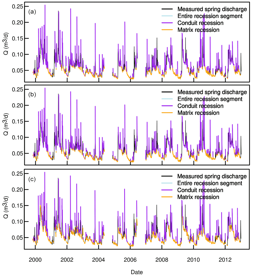
Figure A3 Lehnbachquellen spring discharge hydrograph and extracted recession events recognized by the three REMs: (a) Vogel, (b) Brutseart, and (c) Aksoy.

Figure A4 Saivu spring discharge hydrograph and extracted recession events recognized by the three REMs: (a) Vogel, (b) Brutseart, and (c) Aksoy.

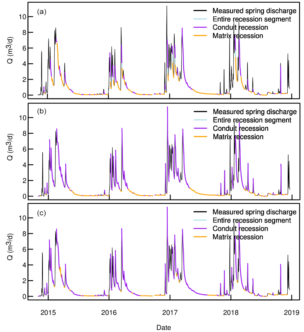
Figure A5 Qachquoch spring discharge hydrograph and extracted recession events recognized by the three REMs: (a) Vogel, (b) Brutseart, and (c) Aksoy.