the Creative Commons Attribution 4.0 License.
the Creative Commons Attribution 4.0 License.
 | 27 Oct 2022
A geostatistical spatially varying coefficient model for mean annual runoff that incorporates process-based simulations and short records
Ingelin Steinsland
Kolbjørn Engeland
We present a Bayesian geostatistical model for mean annual runoff that incorporates simulations from a process-based hydrological model. The simulations are treated as a covariate and the regression coefficient is modeled as a spatial field. This way the relationship between the covariate (simulations from a hydrological model) and the response variable (observed mean annual runoff) can vary in the study area. A preprocessing step for including short records in the modeling is also suggested. We thus obtain a model that can exploit several data sources. By using state-of-the-art statistical methods, fast inference is achieved.
The geostatistical model is evaluated by estimating mean annual runoff for the period 1981–2010 for 127 catchments in Norway based on observations from 411 catchments. Simulations from the process-based HBV model on a 1×1 km grid are used as input. We found that on average the proposed approach outperformed a purely process-based approach (HBV) when predicting runoff for ungauged and partially gauged catchments. The reduction in RMSE compared to the HBV model was 20 % for ungauged catchments and 58 % for partially gauged catchments, where the latter is due to the preprocessing step. For ungauged catchments the proposed framework also outperformed a purely geostatistical method with a 10 % reduction in RMSE compared to the geostatistical method. For partially gauged catchments, however, purely geostatistical methods performed equally well or slightly better than the proposed combination approach. In general, we expect the proposed approach to outperform geostatistics in areas where the data availability is low to moderate.
- Article
(4175 KB) - Full-text XML
- BibTeX
- EndNote


Runoff is defined as the flow of water that is generated from excess rainwater or meltwater, and that flows on the ground surface or within the soil toward a stream (WMO, 1992). Runoff indices of different types (annual runoff, seasonal runoff, maximum runoff) are needed for a variety of purposes, e.g., for designing infrastructure, water supply, and hydropower reservoirs. In spite of the major importance of accurate runoff estimates, the majority of the catchments in the world are ungauged, i.e., runoff measurements for deriving the relevant indices are not available and must be predicted. This is known as the prediction of runoff in ungauged basins problem (PUB) and is a key challenge in hydrology (Blöschl et al., 2013).
There are two main approaches for predicting runoff in ungauged basins: process-based approaches and statistical approaches. In statistical approaches, data from gauged catchments are used to develop a statistical relationship between the observed runoff and relevant variables such as precipitation, temperature, land use, and elevation. The statistical relationship is next used to make predictions for ungauged sites with uncertainty (see, e.g., Viglione et al., 2013; Merz and Blöschl, 2005; Blöschl et al., 2013; Laaha and Blöschl, 2005). In this paper we propose a geostatistical model for mean annual runoff (see, e.g., Gelfand et al., 2010; Cressie, 1993). In the field of hydrology, several geostatistical approaches have been suggested (Roksvåg et al., 2020; Sauquet et al., 2000), but the Top-Kriging method proposed by Skøien et al. (2006) has been shown to be particularly suitable for modeling areal referenced runoff data (Viglione et al., 2013).
Process-based hydrological models are different from statistical models in that they use physical relationships for, e.g., conservation of mass and energy to estimate the flow index of interest. The input variables to the process-based models are variables such as precipitation, temperature, and land use. Data from gauged catchments are used for validation and model calibration (see, e.g., Doherty, 2004; Lawrence et al., 2009). The HBV model is an example of a process-based hydrological approach commonly used to estimate runoff in the Nordic counties (Bergström, 1976). Other process-based models are discussed in Blöschl et al. (2013); Clark et al. (2017); Fatichi et al. (2016).
The ability to account for well-known, physical relationships between the variables is a main benefit of using a process-based model. Geostatistical approaches on the other hand provide uncertainty quantification and are typically better at ensuring a good fit between the runoff data and the model in areas where observations are available. The drawback of the geostatistical approaches is that they often depend on a relatively high gauging density and perform poorly if the underlying process is complex (Wang et al., 2017). Motivated by these benefits and drawbacks, we develop a model that combines geostatistics with a process-based approach.
There is work based on similar ideas in the literature. In Pannecoucke et al. (2020), the authors used a process-based model to simulate flow. Next, empirical variograms were computed based on the simulations and used as input in Kriging, a class of commonly used geostatistical models (see, e.g., Cressie, 1993; Gelfand et al., 2010). The goal was to estimate the contamination level in the soil. In Laaha et al. (2013), Kriging with external drift was used for interpolation of streamflow temperatures, where a physical relationship between mean annual stream temperature and stream gauge altitude was combined with the Top-Kriging approach. Qiu et al. (2018) present a model for mean annual runoff where a Budyko water balance model is combined with a geostatistical approach. In Sauquet (2006) mean annual runoff was estimated by a geostatistical method that incorporated basin characteristics through residual Kriging.
In this paper, we suggest a Bayesian model for mean annual runoff where the observed runoff is used as the response variable and where mean annual simulations from a process-based hydrological model are used as a covariate. To connect the response variable to the covariate, we use a spatially varying coefficient (SVC). In a model with an SVC, the relationship between the response variable and the covariate is allowed to vary within the study area (Gelfand et al., 2003; Ferguson et al., 2009; Hastie and Tibshirani, 1993; Su et al., 2017; Finley, 2011; Lu et al., 2009), i.e., differently from a simple linear regression model where the relationship is restricted to be constant. The motivation behind using an SVC in this work is that we assume that the process-based model is more accurate in some areas than others, and that the accuracy follows regional patterns.
There are several ways to implement an SVC. One option is to simply divide the study area into regions and let a given coefficient have one value for each region, as in Gamerman et al. (2003). Alternatively, the regression coefficient can be modeled as a Gaussian random field (GRF) as described in, e.g., Gelfand et al. (2003). The GRF regionalizes the regression coefficient from locations with data to locations without data according to a spatial dependency structure. In this paper, we adopt the approach from Gelfand et al. (2003). In addition to the SVC, we include an additive spatial effect (GRF). This makes our model able to capture two different dependency structures, e.g., spatial dependency due to both short-range and long-range hydrological processes.
When constructing a runoff map, we find it important to exploit all available data, also data from partially gauged catchments. Partially gauged catchments are catchments that only have short records of data, from a subset of the target period. In this work, we propose to use the approach from Roksvåg et al. (2020) to preprocess the short records before further analysis with the SVC model. The preprocessing procedure fills in missing annual observations, and has been shown to work well for flow indices and study areas that are dominated by runoff patterns that are repeated over time (Roksvåg et al., 2020). After the preprocessing, the short records are incorporated into the SVC model through an observation likelihood that supports data from both fully and partially gauged catchments with different observation uncertainties.
The main objective of this paper is to present a framework for mean annual runoff estimation that exploits several data sources: precipitation data, temperature data, and land use through the process-based covariate as well as data from fully gauged and partially gauged catchments through the observation likelihood. The framework is made computationally feasible by using state-of-the-art statistical methods such as INLA (integrated nested laplace approximations) and the SPDE (stochastic partial differential equation) approach to spatial modeling (Rue et al., 2009; Lindgren et al., 2011). These tools enable fast and approximate inference for Bayesian spatial models.
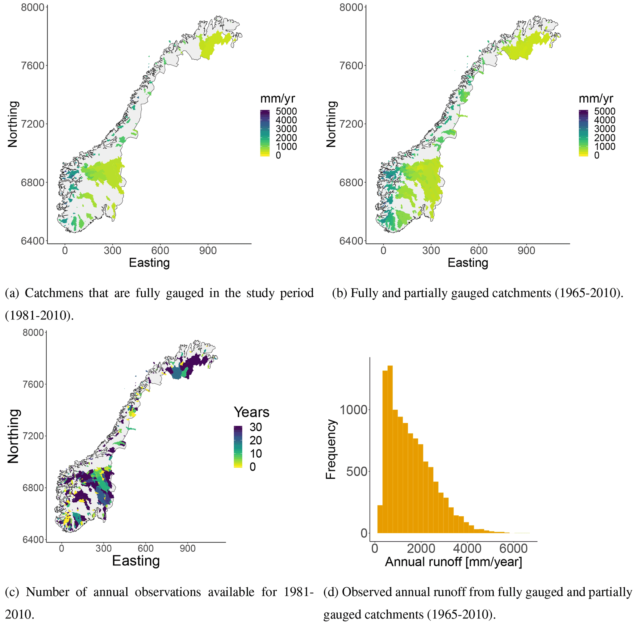
Figure 1Mean annual runoff for Norwegian catchments (a–b) derived from daily streamflow observations. There are annual runoff data available from 127 fully gauged catchments and from 284 partially gauged catchments. We plot subcatchments in front of larger, surrounding catchments in all of our plots. (c) Number of annual observations that are available for each catchment in the study period (1981–2010). If the number is equal to 0, it means that there is at least one annual observation available from 1980 or earlier years, more specifically between 1965 and 1980. The reference system used is UTM33N EUREF89 with coordinates given in kilometers. (d) Annual observations for all catchments and years.
To evaluate the model, we estimate mean annual runoff in Norway. Simulations of mean annual runoff produced by the process-based HBV model are used as a covariate. The evaluation assesses the model's ability to
-
produce a satisfactory gridded map for mean annual runoff with uncertainty quantification.
-
predict runoff for partially gauged and ungauged catchments.
As reference models we use a purely process-based model (the HBV model) and a purely geostatistical model (Top-Kriging).
In the next section (Sect. 2), we present the available Norwegian runoff data and model input. Here, we describe the process-based HBV model and how it was used to produce simulations on a grid. In Sect. 3, we introduce the background theory, relevant statistical models, and notation. Further, in Sect. 4, we present the suggested mean annual runoff model. The experimental set-up for evaluating the model is presented in Sect. 5, and in Sects. 6 and 7 we present and discuss our results. Finally, we summarize and conclude in Sect. 8.
2.1 Runoff data
To evaluate the proposed approach, we use mean annual runoff data from Norway from the time period 1981–2010 provided by the Norwegian Water Resources and Energy Directorate (NVE). The mean annual runoff observations have the unit mm yr−1 and were derived by aggregating daily measurements of streamflow from Norwegian catchments, for hydrological years that start 1 September and end 31 August. If a catchment had less than 365 daily observations for a specific year, this annual observation was considered missing.
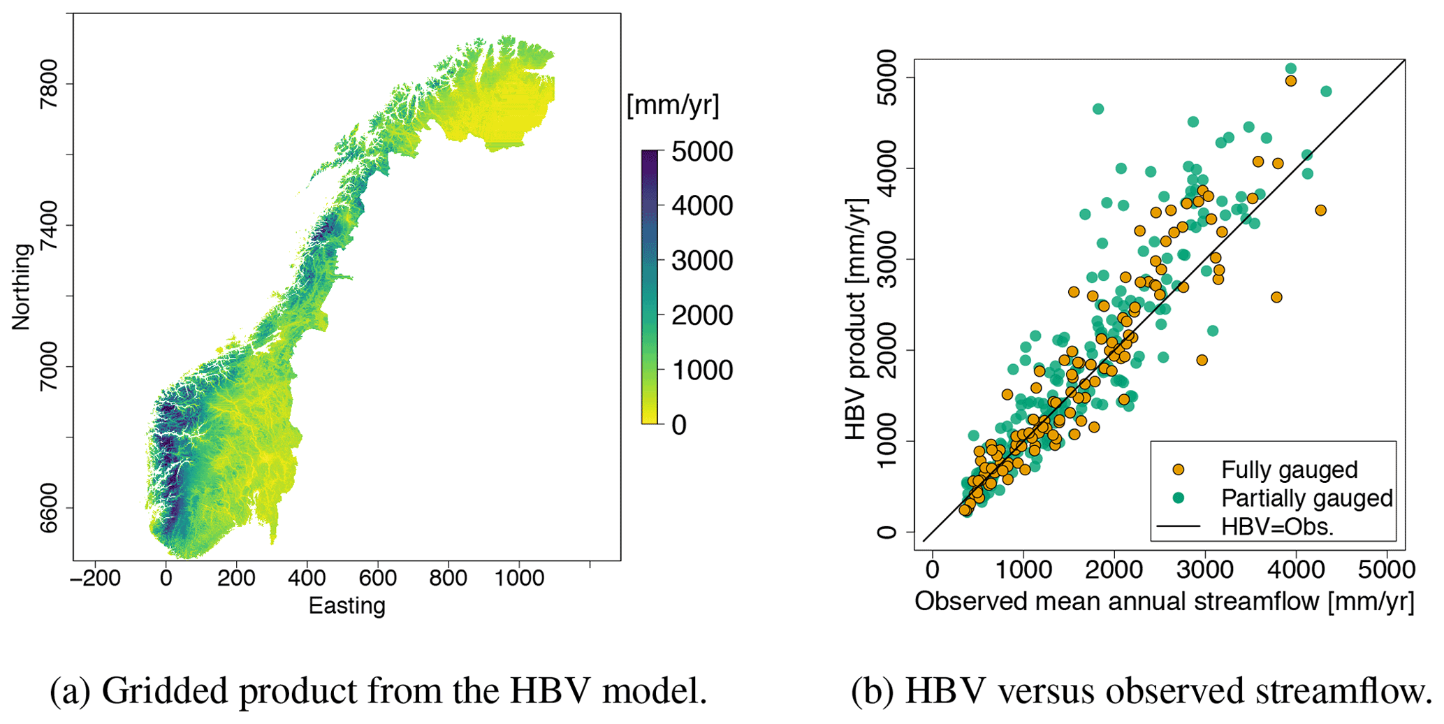
Figure 2A mean annual runoff (1981–2010) product simulated by the HBV model (a). The product is delivered on a 1×1 km grid. (b) The fit between the HBV product and the actually observed streamflow for the fully gauged (orange) and partially gauged catchments (green).
Furthermore, we only use data from catchments where human activities have had negligible impact. To select catchments, we used the regulation capacity of hydropower reservoirs as a criterion, i.e., the ratio between the mean annual runoff and the reservoir storage capacity. If this ratio was smaller than 0.2 for a catchment, the catchment was included in the analysis, assuming that the annual changes in water storage are small compared to the annual inflow volume. The assumption was also checked for a subset of the target catchments, and we found that the standard deviation of annual changes in reservoir storage was less than 2 % of annual inflow.
After performing the data-cleaning procedure, there were data available from 127 catchments that were fully gauged in the 30-year target period, 1981–2010. The average runoff for these catchment are shown in Fig. 1a with the unit mm yr−1. In addition, there were annual observations available from 284 partially gauged catchments. These had at least one annual runoff observation between 1965 and 2010 and their observed mean annual runoff is shown in Fig. 1b. The number of annual observations for each of these catchments is shown in Fig. 1c. The average record length is 12 years (median 9.5 years) for the period 1981–2010, but 15 years (median 16 years) if we consider the longer period from 1965 to 2010.
In Fig. 1d we show the annual runoff observations for individual years. Here, it is apparent that the spatial variability of the Norwegian annual runoff is large. The mean annual runoff follows the spatial pattern we see in Fig. 1b, with high values in the western part of the country and low values in the eastern part each year. The pattern is mainly caused by the orographic precipitation that occurs when humid winds from the Atlantic Ocean are elevated over the mountains in western Norway. This gives large precipitation amounts in the western parts of the country, while the eastern parts are left in the rain shadow.
2.2 Gridded simulations from the HBV model
We use a gridded mean annual runoff product simulated by the HBV model as a covariate in a geostatistical model. The first application of the gridded HBV model in Norway is reported in Beldring et al. (2002), and it is applied in several studies to assess runoff and water balance in Norway (e.g., in Borgvang et al., 2006; Skarbøvik et al., 2009; Hanssen-Bauer et al., 2017). In this case, we use a data product that was already available from the data provider NVE's database (see Fig. 2a). The product covers the whole country of Norway, and smaller parts of its neighboring countries such that catchments that cross the Norwegian border can be included. The product is delivered on a 1×1 km grid and is based on simulations of daily time series of runoff. Interpolated temperature and precipitation were used as input together with gridded land use characteristics. Daily simulated time series of runoff were aggregated to mean annual runoff (mm yr−1) for our reference period 1981–2010. We refer to Bergström (1976); Sælthun (1996); Lindström et al. (1997) for detailed descriptions of the algorithms used in the HBV model, and to Beldring et al. (2002) for details about the specific product in Fig. 2a.
To determine the parameters in the HBV model, it is common to perform a global calibration procedure based on streamflow observations. The aim is to minimize global bias and the errors. When producing the map in Fig. 2a, streamflow observations from 141 fully gauged catchments were used for the calibration. It should be noted that since we use the HBV product that was already available from the data provider NVE's database, the calibration catchments are not necessarily the same catchments we use in our geostatistical model. See Beldring et al. (2003) for details about the calibration procedure.
As the parameters are calibrated globally, there are still local biases in the HBV model's predictions relative to the observed streamflow. This can be seen in Fig. 2b where we depict the difference between the mean annual runoff provided by the HBV model (Fig. 2a) and the observed mean annual runoff (Fig. 1). We see that the fit is close to linear for catchments with low observations of mean annual runoff. For observations over 2000 mm yr−1, the HBV model tends to overestimate the mean annual runoff. By using the proposed geostatistical approach, we aim to produce a runoff map that improves the fit.
3.1 Bayesian statistics and hierarchal modeling
We take a Bayesian approach to statistics (see, e.g., Gelman et al., 2004; Casella and Berger, 1990). In Bayesian statistics, the random variable x is associated with a probability distribution that expresses what we know about the underlying process of interest. Before the statistical analysis is conducted, our beliefs are expressed mathematically through a so-called prior distribution, denoted π(x). This can be constructed based on expert knowledge about the process under study or based on earlier experiments. The goal of the Bayesian analysis is to update π(x) based on data y. This can be done by using Bayes' formula:
where π(y|x) is the observation likelihood that connects the observed values to the target variable x. The resulting distribution π(x|y) is called the posterior distribution, and represents what we know about the underlying process based on our data. One of the benefits the Bayesian framework is that a full uncertainty specification for the target variable x is directly available through the posterior distribution. If a point prediction is of interest, the median, mean, or mode of the posterior distribution π(xi|y) can be used as a summary statistic, for any xi∈x.
The geostatistical runoff model we propose is also a hierarchical model. Hierarchical models make it possible to formulate rather complex models by specifying a set of simpler models (see, e.g., Banerjee et al., 2004). For example, if we model runoff, we can assume that the true underlying runoff x is observed through data y that are associated with some measurement uncertainty. Further, we can assume that the runoff has some spatial or temporal variability that can be modeled by a statistical distribution with parameters . Mathematically the above model can be expressed in three stages: the observation likelihood, , the latent model or process model π(x|θ), and the prior distribution π(θ).
3.2 Gaussian random fields (GRFs)
Random fields (RFs) are often used to model spatial correlation in geostatistical models for hydrological variables (see, e.g., Sauquet et al., 2000; Skøien et al., 2006; Roksvåg et al., 2020). In this paper, we use GRFs to model the spatial dependency of runoff. A continuous field defined on a spatial domain 𝒟 is a GRF if , where is a multivariate normal distribution with expected values given by vector μ and covariance given by the covariance matrix Σ (Cressie, 1993). The covariance matrix specifies the dependency structure of the variable of interest. Typically, a matrix element (i,j) is generated by using a known covariance function C(ui,uj) that models the correlation of the target variable between two locations Cov(x(ui),x(uj). The covariance function often has a marginal variance parameter σ2 and a range parameter ρ that characterize the underlying spatial field. The marginal variance describes the spatial variability of the target variable, while the range is a measure of how correlation decays with distance.
In our work we use a stationary Matérn covariance function to model the covariance of mean annual runoff. The Matérn covariance function is defined as
where Kν is the modified Bessel function of second kind and order ν>0, Γ(⋅) is the gamma function, and is the Euclidean distance between the two locations . Further, σ2 is the marginal variance and κ is a scale parameter (Guttorp and Gneiting, 2006). Empirically, it has been shown that the parameters ν and κ can be used to express the spatial range as
where ρ is defined as the distance at which the correlation between two locations has dropped to 0.1 (Rue et al., 2009).
The reason for using a Matérn covariance function in our work is that it makes it possible to use the stochastic partial differential equation (SPDE) approach to spatial modeling (Lindgren et al., 2011). The SPDE approach is described in Sect. 4.6 and is used to make the proposed model computationally feasible. In addition, the Matérn class of covariance functions has many useful properties and Stein (1999) advises its use. In the runoff model that follows, the σ2 and ρ parameters are estimated, while the parameter ν is fixed and set equal to 1. The reason is that ν is often hard to identify in typical applications, and ν=1 is the default choice in the INLA software that is used to fit our model (Lindgren et al., 2011; Blangiardo and Cameletti, 2015).
3.3 Existing geostatistical models used for runoff interpolation
3.3.1 Top-Kriging
Kriging approaches are commonly used for spatial interpolation. In Kriging approaches, the variable of interest is modeled as a random field x(u), and an estimate of the random field x(u0) at an unobserved location u0∈ℛ2 can be expressed as the weighted sum of a set of observations , i.e., as
where λi for are interpolation weights that must be determined (Cressie, 1993). The interpolation weights are found by minimizing the mean squared error between the estimate and the true x(u0), and assuming zero mean expected error.
The estimation of the Kriging weights requires evaluations of the covariance function (or variogram). The Top-Kriging approach (Skøien et al., 2006) treats runoff observations as areal referenced when computing the covariance, unlike other standard Kriging approaches. This way, observations from a subcatchment can be weighted more than observations from a nearby, non-overlapping catchment. Top-Kriging is one of the leading methods for interpolation of runoff (Viglione et al., 2013; Blöschl et al., 2013), and we hence use it as a geostatistical reference method.
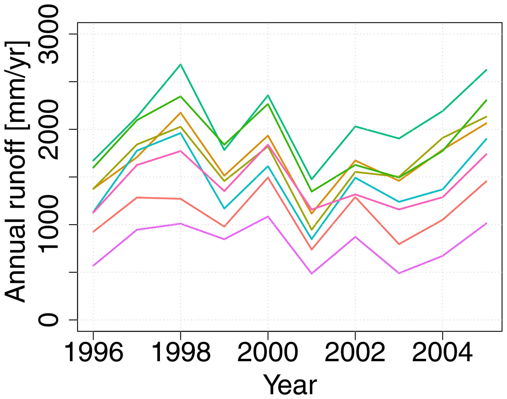
Figure 3Time series of annual runoff for eight catchments in Norway that are located in the same region. The time series are almost parallel, indicating that the spatial patterns of runoff are repeated over time.
3.3.2 Geostatistical method for exploiting short records
To include short records in our model, we use the method from Roksvåg et al. (2020) as a preprocessing step. The method is a Bayesian hierarchical geostatistical model that is particularly suitable for filling in missing data for catchments that have short records of data relative to neighboring catchments. It models several years of (annual) runoff simultaneously through two GRFs: one that describes the long-term spatial variability, and one that describes year-dependent spatial effects. The method weights the two GRFs relative to each other. If long-term effects dominate, the potential information stored in short records is large.
The method from Roksvåg et al. (2020) has its benefits when runoff follows spatial patterns that are repeated over time. This is the case for our target variable, Norwegian annual runoff, that is driven by orographic precipitation caused by repeated wind patterns from the Atlantic Ocean (Stohl et al., 2008). Example data from Norway are shown in Fig. 3. The repeated spatial pattern is recognized in that the ranking of the catchments, from wet to dry, is approximately constant. For variables and areas that are not driven by such characteristic spatial patterns, the method in Roksvåg et al. (2020) provides a more classic form of spatial interpolation, similar to Kriging.
The method from Roksvåg et al. (2020) is available for both point and areal referenced data. In this application, we use it as a point referenced model to save computational time, and the catchments centroids are used as the observation locations. We expect the point referenced model to be sufficiently good for our study for two reasons: (1) We are only using the model to make predictions for catchments where we have at least one annual observation and (2) we are not going to use the posterior uncertainty of the model. The results in Roksvåg et al. (2020) show that the point referenced model gives results that are similar to the areal referenced model for partially gauged catchments when we are only interested in posterior means and not posterior standard deviations.
We now present our proposed geostatistical Bayesian hierarchical model for mean annual runoff and its three stages: a process model, an observation model, and prior distributions.
4.1 Process model for true mean annual runoff
4.1.1 Point model
Assume that mean annual runoff (mm yr−1) is a continuous process that occurs for any point u∈ℛ2 in the landscape. We model the true mean annual runoff q(u) at a point location or a (small) grid cell u as
where β0 is an intercept parameter, the variable h(u) is a covariate that contains the simulated value generated by a process-based hydrological model at point location or a grid cell u, and (β1+α(u)) defines an SVC. The SVC consists of one component β1 that is fixed in space and one component α(u) that is location dependent. The spatial variability of α(u) is introduced by modeling it as a stationary Matérn GRF field given a range parameter ρα and a marginal standard deviation parameter σα. This way the relationship between the true mean annual runoff q(u) and the simulations made by the hydrological model h(u) can vary in the study area. The α(u)h(u) component also ensures a model where the mean and the variance of runoff can be inhomogeneous in space. We use mean annual runoff simulations from the HBV model as input in h(u), but gridded simulations from any relevant hydrological model can be applied.
The SVC β1+α(u) in Eq. (5) models a similar dependency structure as we would get from ratio interpolation, i.e., interpolation of the ratio between the observed runoff and a process-based covariate. Ratio interpolation is a method that has been used before in, e.g., Beldring et al. (2002) to improve the results of a process-based model. In our runoff model, we also include an additional spatial effect x(u) that is assumed to be conditionally independent of α(u) a priori, given the underlying model parameters. Like α(u), x(u) is modeled as a GRF with a stationary Matérn covariance structure, but with range and marginal standard deviation ρx and σx, respectively. The GRF x(u) models a dependency structure similar to what we would get from residual interpolation. Residual interpolation was used in, e.g., Merz and Blöschl (2005) to improve the results from an initial multiple linear regression model.
4.1.2 Areal model
In Eq. (5) we modeled runoff as a point referenced process, but in practice, runoff is observed through streamflow observations that are linked to catchment areas. We thus introduce a model for the true runoff inside a catchment area 𝒜. This is given by
where q(u) is the mean annual point runoff from Eq. (5) and is the area of the target catchment. The true areal runoff is given by the average point runoff integrated over the catchment area. In practice, it is not computationally feasible to perform the integration in Eq. (6). Our solution is to approximate the integral in Eq. (6) by a sum. This is done by discretizing catchment 𝒜 into a regular grid ℒ𝒜 and defining the mean annual runoff in catchment 𝒜 as
where n𝒜 is the number of grid nodes in the discretization of catchment 𝒜. The areal formulation in Eq. (7) assumes a linear aggregation of runoff over the grid nodes included in the catchment discretization. This is reasonable for variables that are approximately mass conservative over catchment areas, like the mean annual runoff.
We have now defined our final process model for runoff, which is an areal model (Eq. 7) that builds on a point specification of the underlying process (Eq. 5). From Eqs. (5) and (7), we see that in order to calculate Q(𝒜) we need the simulated values produced by the hydrological product, h(u), for all grid nodes inside 𝒜. Consequently, the catchment discretization should follow the same discretization as the gridded hydrological product. In our case the HBV product came on a regular grid with 1 km spacing. The selected grid should be dense enough to ensure an accurate approximation for the true areal runoff in Eq. (7).
4.2 Observation model for mean annual runoff
The true mean annual Q(𝒜) runoff is not observed directly, but through areal referenced streamflow observations with uncertainty. We model the observed mean annual runoff in catchment 𝒜i as
where Q(𝒜i) is the areal referenced true mean annual runoff from Eq. (7), and the ϵi values are independent and identically distributed error terms with prior . The parameter σy describes the underlying standard deviation, while the si values are fixed, predetermined scales that allow each observation to have its own measurement uncertainty. This way heteroscedasticity can be introduced in a simple way. The values of the scales si are further specified in Sect. 4.3.
In Eqs. (5) and (8), runoff is modeled through Gaussian components, which means that there is a risk of obtaining negative runoff predictions. To avoid negative runoff predictions, we could log transform the runoff data before performing the analysis, but this requires that we model the runoff observations as point referenced instead of areal referenced. The reason is that the sum in Eq. (7) does not make sense for log-transformed runoff data. Another option is to use a log-Gaussian likelihood and log-GRFs for x(u) and α(u), such that predictions for x(u) and α(u) are always positive. In this work, however, we keep the areal formulation and the more interpretive versions of the spatial fields. For Norwegian mean annual runoff, negative predictions are quite unlikely anyway, since the observations are far from zero. The areal formulation also gives a more realistic uncertainty model and lets us constrain the mean annual runoff not only at certain gauging points, but over catchment areas.
4.3 Prior distributions for model parameters
The third stage of the proposed hierarchical model for mean annual runoff consists of the prior distributions of the seven model parameters, . In this section we specify the prior distributions we have used. Most of the priors are constructed such that they are suitable for modeling Norwegian mean annual runoff, and should be revised if the model is used for other flow indices and/or study areas.
We start by constructing a prior for the measurement uncertainty . As stated in the previous subsection, the variance parameter is scaled with a fixed an predetermined scale si such that each observation of mean annual runoff can have its own measurement uncertainty. A variance that changes with the observed value is reasonable when modeling Norwegian mean annual runoff, because the variability of runoff across the country is large. The observed annual runoff varies from around 500 to 4000 mm yr−1. With this in mind, we specify the scales si under the assumption that larger observations of mean annual runoff have larger measurement uncertainties than smaller observations of mean annual runoff. This is obtained by modeling the scales as
where yi is the observed mean annual runoff in catchment 𝒜i in mm yr−1. The number 0.025 was chosen based on expert opinions from the data provider NVE. A standard deviation around 2.5 % is assumed to be reasonable. The scales are divided by a factor of 1000 to get suitable values for the quantity .
We next specify a prior distribution for the standard deviation parameter σy. For this, we use a penalized complexity (PC) prior as suggested by Simpson et al. (2017). The PC prior is chosen because it has convenient mathematical properties. It controls for overfitting by penalizing the increased complexity that arises when a model deviates from a simpler, less flexible base model. The PC prior for the precision τ (or the inverse variance) of a Gaussian effect is given by
where λ controls the deviation penalty. The parameter λ can easily be specified through a probability α and a quantile u as , where σ0>0, and , where is the standard deviation of the Gaussian effect. For our application, we let α=0.1 and σ0=1500 mm yr−1, and define the PC prior for σy as follows:
This means that the prior probability that σy is larger than 1500 mm yr−1 is 10 %. However, recall that the measurement variance of yi is determined by and not by alone. With the scales in Eq. (9) and the PC prior for σy in Eq. (11), a prior 95 % credibility interval for the observation standard deviation for the mean annual runoff is (0.04,6) % of the corresponding observed value yi for a catchment 𝒜i, with prior mean centered around 2.5 %. Values in this range are reasonable and reflect the data provider NVE assumptions about the uncertainty of the Norwegian mean annual runoff observations. By creating a relatively narrow prior for , we influence the model to reproduce the actually observed runoff for catchments where we have data.
In Fuglstad et al. (2019) the PC prior framework is used to develop an informative, joint prior for the range and the marginal variance of a GRF. We use this prior for the spatial marginal standard deviation σα and the spatial range ρα for the SVC component α(u). The prior is specified through the following probabilities and quantiles:
where we a priori assume that the spatial range of the SVC is larger than 20 km. This is a reasonable assumption, as it is likely that locations that are closer than 20 km are correlated when it comes to annual runoff. Based on Fig. 2b we assume a priori that the ratio between the response variable Q(⋅) and the covariate h(⋅) varies with a factor that has a standard deviation smaller than 2.
Likewise, we use the PC prior from Fuglstad et al. (2019) to specify a joint prior for the marginal standard deviation σx and the spatial range ρx of the spatial field x(u). We use the following probabilities and quantiles:
Here, we again assume a priori that the range is larger than 20 km by taking the size of the study area into account. The prior probability that the standard deviation of the Norwegian mean annual runoff is larger than 2000 mm yr−1 is set to a low probability. We find this reasonable as most of the mean annual observations are between 500 and 4000 mm yr−1.
For the two parameters β0 and β1 we use weakly informative normal prior distributions, with 0 mean and standard deviation 10 000.
4.4 Preprocessing step for incorporating short records (PP)
We now present an extension of the model that makes it possible to include short records in the proposed mean annual runoff model. The extension is based on using the geostatistical model described in Sect. 3.3.2 to fill in missing annual observations and/or augment short records for the partially gauged catchments. After filling in the missing years, we get a preliminary estimate of the mean annual runoff for these catchments. These estimates are next used as observations yi in the SVC model together with data from fully gauged catchments.
The observations yi we obtain from the preprocessing step are probably more uncertain than the data from the fully gauged catchments. To reflect this, we use a different prior for the observation uncertainty for the preprocessed data compared to that of the fully gauged catchments. Recall that the prior observation variance for a fully gauged catchment was given by where si was a fixed predetermined scale given by . For partially gauged catchments we replace this scale by
where PP denotes that observation yi from catchment Ai is preprocessed. In practice, each partially gauged catchment could have its own scaling factor, e.g., one that depends on record length, but in this demonstration we use the same scaling factor for all partially gauged catchments for simplicity. With the scales in Eq. (14), a 95 % credible interval for the prior standard deviation becomes (0.1,24) % of the observed value for the partially gauged catchments, while it is only (0.04,6) % for data from fully gauged catchments.
The preprocessing step lets us exploit streamflow observations from catchments that have down to one annual observation, and the short record could also be from the period before the study period starts. As explained in Sect. 3.3.2, the preprocessing step is expected to contribute positively to the model if the flow index of interest is driven by repeated spatial patterns over time. If this is not the case, the preprocessing step only performs classic geostatistical spatial interpolation and can be skipped to save time.
4.5 Full model specification
We have proposed a model for mean annual runoff that can incorporate process-based simulations and data from fully gauged and partially gauged catchments. The full model can be specified in a hierarchical model with three levels, where the first level is the observation likelihood,
the second level is the latent field,
and the third level is the prior model,
In Eqs. (15–17), y is a vector containing all observations of mean annual runoff for catchments . The function I(⋅) is an indicator function that is equal to 1 if its argument is true and 0 otherwise, allowing for data from both fully gauged and partially gauged catchments. We see that the likelihood specification for the fully and partially gauged catchments is the same, except for the difference in measurement uncertainty expressed through si and . The variable x is a vector that contains all the latent variables, i.e., the two GRFs and for all grid nodes that are used in the discretization of the catchment areas. Finally, θ is a parameter vector that contains β0, β1, , and σα.
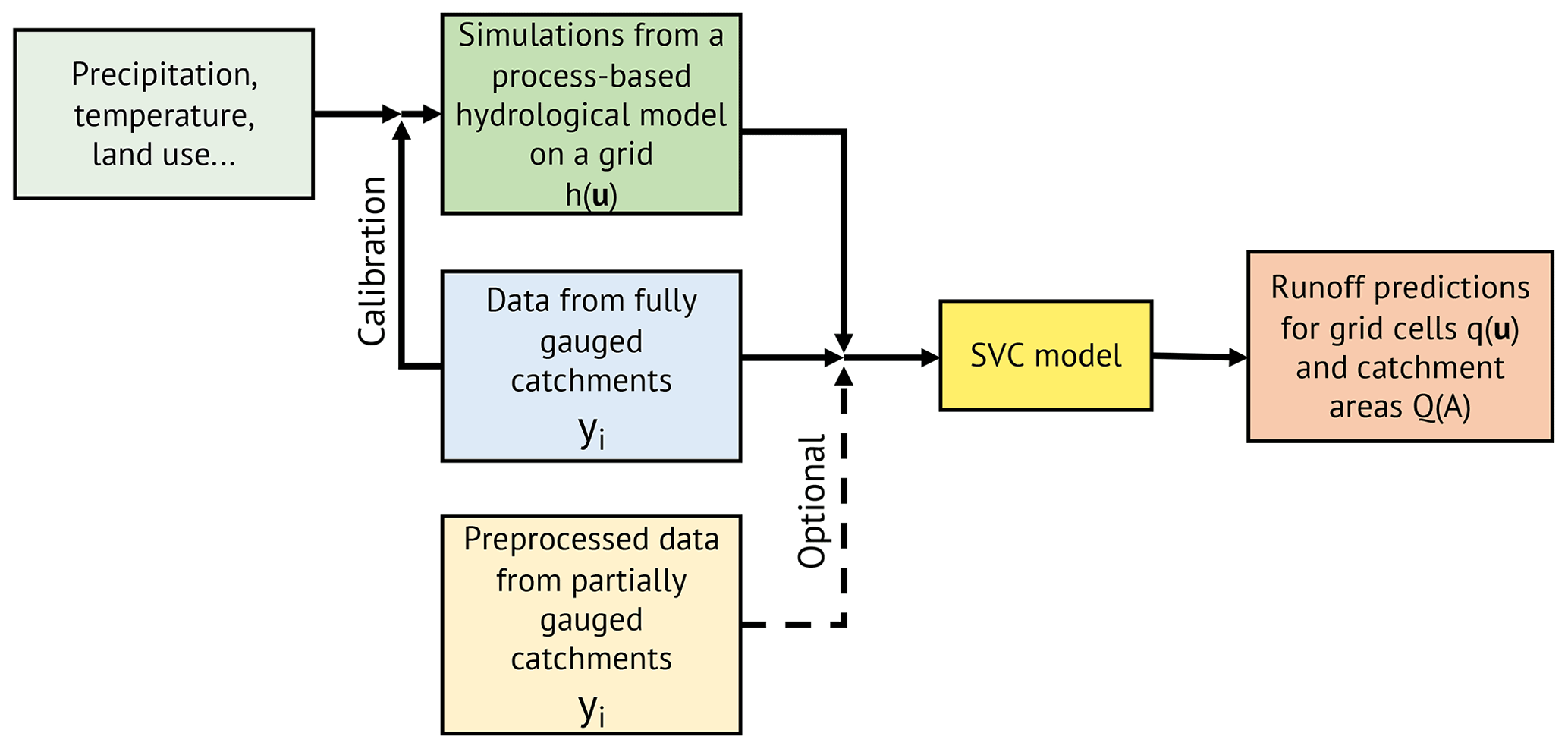
In Fig. 4 we depict the proposed approach in a flow chart. We emphasize that the SVC model can be applied with or without incorporating preprocessed short records. To mark results where preprocessed data are involved, we will use the subscript PP in the remainder of the paper.
4.6 Approximate inference
To make runoff predictions q(u) and Q(𝒜), we need to estimate x and θ given data y. Traditionally, inference on Bayesian hierarchical models has been done by using Markov chain Monte Carlo (MCMC) methods (Gamerman and Lopes, 2006). However, the computational complexity of carrying out an MCMC procedure is large when the dimension of x is large. To make the proposed model computationally feasible, we use integrated nested Laplace approximations (INLA). The INLA methodology was suggested by Rue et al. (2009) and is developed for making approximate Bayesian inference on latent Gaussian models (LGMs), i.e., hierarchical models where the latent field x is Gaussian. As the latent variables contained in x are given Gaussian prior distributions considering the underlying model parameters, this requirement is fulfilled for our SVC model. The INLA methodology is based on Laplace approximations, sparse matrix calculations, and numerical integration schemes, and we refer to Rue et al. (2009) for details.
Furthermore, it is computationally challenging to make statistical inference on spatial models. The reason is that it takes time to perform matrix operations on the covariance matrices of GRFs when there are many target locations. To ensure fast inference for our two-field model, we use the SPDE approach to spatial modeling, as suggested by Lindgren et al. (2011). The approach is based on the fact that a GRF with Matérn covariance matrix can be expressed as the solution of a stochastic partial differential equation (Whittle, 1954, 1963). An approximate solution of the SPDE can be obtained by using the finite element method (see, e.g., Brenner and Scott, 2008), where the resulting approximation is given on a triangular mesh. This mesh approximation gives computational benefits compared to the exact GRF solution, and enables fast inference for spatial models (Rue and Held, 2005; Rue et al., 2009).
The INLA and SPDE methodologies are implemented in the R-package INLA, which since its introduction has been used within a range of different fields. See Opitz et al. (2018); Guillot et al. (2014); Myrvoll-Nilsen et al. (2020); Bakka et al. (2018); Blangiardo and Cameletti (2015); Khan and Warner (2018) and https://www.r-inla.org/ (last access: 18 October 2022) for some examples. The approximations used in the SPDE and INLA framework are in general accurate and reliable when the likelihood is Gaussian, as in this application, and as long as the triangular mesh used in the finite element computations is dense enough relative to the spatial variability of the target variable. A mesh that is too coarse could lead to unrealistic results such as negative runoff.
5.1 Making a gridded mean annual runoff map for 1981–2010
To evaluate the proposed approach for runoff estimation, we use the SVC model to produce a gridded mean annual runoff map for the period 1981–2010 for the same 1×1 km grid as the HBV model was delivered on (Fig. 2a). For the fully gauged catchments, we use the data from 1981 to 2010 to compute the mean annual runoff yi, while for the partially gauged catchments we use the preprocessing step on the short records (PP) before further analysis. In the preprocessing step, data from 1965 to 2010 were used to estimate the mean annual runoff for the period 1981–2010.
We evaluate the model in terms of whether the new map represents an improvement compared to the original HBV map. This is done by investigating how well the new map fits with the observed runoff from the fully gauged and partially gauged catchments.
In addition to the experiment described above, we repeated the experiment, but omitted partially gauged catchments and short records from the analysis. This was done to show that the SVC model works regardless of the preprocessing step. See Appendix A for the results.
5.2 Cross-validation for ungauged and partially gauged catchments
We next evaluate the framework's ability to perform accurate mean annual runoff for ungauged and partially gauged catchments. This is done by a cross-validation assessment, where we make predictions for the 127 fully gauged catchments in Fig. 1a. The 127 fully gauged catchments are divided into five groups or folds. The first four folds have 25 target catchments, while the fifth fold has 27 target catchments. In turn, the streamflow data corresponding to each fold are removed from the dataset, while the remaining observations are used to predict the mean annual runoff for these catchments for the period 1981–2010. The likelihood consists of preprocessed observations from partially gauged catchments and observations from fully gauged catchments, i.e., around 400 observation catchments in total. Recall that we do not calibrate the HBV model for each cross-validation fold, as the HBV product was a pre-made product.
In our evaluation, we compare the predictive performance of the SVC model with the process-based HBV model. The original simulations from the HBV model shown in Fig. 2a are hence used as they are. For evaluation purposes, the values in Fig. 2a are aggregated and averaged to catchment runoff for the catchments in Fig. 1.
We also compare our approach with the purely geostatistical Top-Kriging (TK) approach described in Sect. 3.3. Here, we fit a covariance model based on a multiplication of a modified exponential and fractal variogram model to the mean annual runoff data. This is the default variogram model in the R-package rtop (Skøien, J.O., 2018). As for the SVC model, data from both fully gauged catchments and preprocessed partially gauged catchments are used as input, and we mark the TK results by TKPP to emphasize that preprocessed data are used. For fully gauged catchments, the standard deviation of the observations is set to 2.5 % of the observed value yi in the TK approach, while for partially gauged catchments the standard deviation is set to 10 % of the observed value. The aim is to make the TK results as comparable as possible to the SVC model results.
In addition to evaluating TK and the HBV model, we include prediction results from the preprocessing step (PP) alone, without performing any further analysis. The PP predictions come from the purely geostatistical method described in Sect. 3.3.2 and can be used to make predictions in both ungauged and partially gauged catchments. We include the PP results to make the TK and SVC results more transparent. These two methods use the PP results as input data for the partially gauged catchments (see Sect. 4.4).
The described cross-validation procedure is first performed when the 127 target catchments are treated as ungauged. We have the following setting:
-
Ungauged catchments (UG): The target catchments in each cross-validation fold are treated as totally ungauged (UG) in the time period of interest (1981–2010) and their observations are removed from the dataset. Observations from fully gauged catchments from other cross-validation groups (1981–2010) and observations from partially gauged catchments (1965–2010) are used to make predictions.
We also evaluate the predictive performance of the model when the 127 target catchments are treated as partially gauged by conducting the following experiment:
-
Partially gauged catchments (PG): The target catchments in each cross-validation are allowed to have three annual observations in the study period (1981–2010). These are randomly drawn from the period 1981–2010. The remaining 27 observations are removed (and observations from before 1981). Observations from nearby fully gauged catchments (1981–2010) and partially gauged neighboring catchments (1965–2010) are included in the likelihood as before.
The same cross-validation groups are used for all experiments, such that the results become comparable across methods. The randomly drawn short records of 3 annual observations are also the same for TK and the SVC approach.
In addition to the above experiments, we carried out a cross-validation for the UG setting when omitting catchments with short records and preprocessed data. These results can be found in Appendix A.
5.3 Evaluation scores
To evaluate the accuracy of the predictions obtained from the cross-validation, we use three evaluation scores. These are the root mean square error (RMSE), the absolute normalized error (ANE), and the Nash–Sutcliffe model efficiency coefficient (NSE), which are defined as
and
Here, is the predicted mean annual runoff in catchment 𝒜i, yi is the corresponding observed value, and denotes the average observed mean annual runoff over all study catchments . For the suggested SVC model, we use the posterior mean of Q(𝒜i) as the predicted value (Eq. 7). As a summary statistic for ANEi, we use the average ANEi over all catchments . A low average ANEi or a low RMSE corresponds to accurate predictions. The NSE on the other hand takes values between −∞ and 1, and the closer the model efficiency is to 1, the more accurate the model is. The ANE and the NSE are different from the RMSE in being scale-independent evaluation scores.
The three aforementioned scores are suitable for evaluating prediction bias, but they do not evaluate the models' uncertainty quantification. For this reason we introduce two additional evaluation scores: the continuous ranked probability score (CRPS) and the 90 % coverage. The CRPS is generally given by
where y is the observed value and F(⋅) is the predictive cumulative distribution (Gneiting and Raftery, 2007). The CRPS takes the whole posterior distribution F(⋅) into account, unlike RMSE, ANE, and NSE that only consider point values. A low CRPS corresponds to an accurate prediction, and the CRPS increases if the observed value y falls outside the posterior predictive distribution F(⋅). In this application, we assume F(⋅) to be Gaussian distributed with the expected value given by the predicted mean annual runoff and standard deviation equal to the corresponding predictive standard deviation. The Gaussian assumption should be reasonable, as the posterior distributions of the predicted runoff typically are symmetric with light tails. We use the average CRPS over the 127 fully gauged catchments as a summary score.
The 90 % coverage is defined as the probability that 90 % of the observed values are covered by the corresponding 90 % posterior prediction intervals. This probability is computed empirically based on the predictions for the 127 fully gauged catchments, assuming that the SVC and TK predictions follow a Gaussian distribution with mean and standard deviation from the SVC or TK model. If the empirical probability is close to 90 %, it suggests that the model provides an appropriate uncertainty quantification.
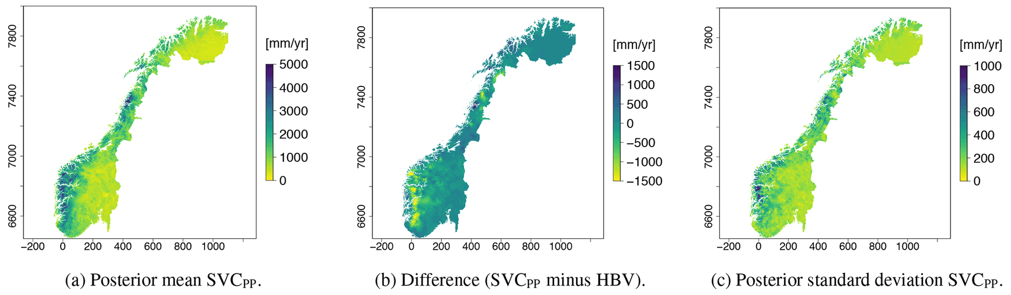
Figure 5Posterior mean of q(u) for all grid nodes u (a), difference between the new map and the original HBV map (new–old, b) and posterior standard deviation of q(u) (c).
6.1 Gridded mean annual runoff map for 1981–2010
In Fig. 5a we present the runoff map produced by the SVCPP approach. The difference between the new map and the original HBV product is depicted in Fig. 5b, while the map's uncertainty is shown in Fig. 5c. Figure 5b shows that the SVCPP map gives lower values of mean annual runoff in western Norway compared to the original HBV map. The difference is around 700–1500 mm yr−1. In eastern Norway, the original HBV map and the SVCPP map are quite similar, both in the southeast and northeast. In the area around the glacier Svartisen, located by y-coordinate 7400 on the map, the mean annual runoff of the SVCPP map is lower than the mean annual runoff of the original HBV map. The difference here is around 1500 mm yr−1.
We see from Fig. 5a that the SVCPP map preserves most of the details provided by the original gridded HBV product in Fig. 2a. The runoff map produced by SVCPP also looks visually good without, e.g., unrealistic jumps or obvious discontinuities. One exception is a line or discontinuity close to the Finnish border, northeast in Fig. 5a, but this line was already present in the original HBV product in Fig. 2a.
Table 1Posterior median (0.025 quantile, 0.975 quantile) for the parameters of the SVCPP model.
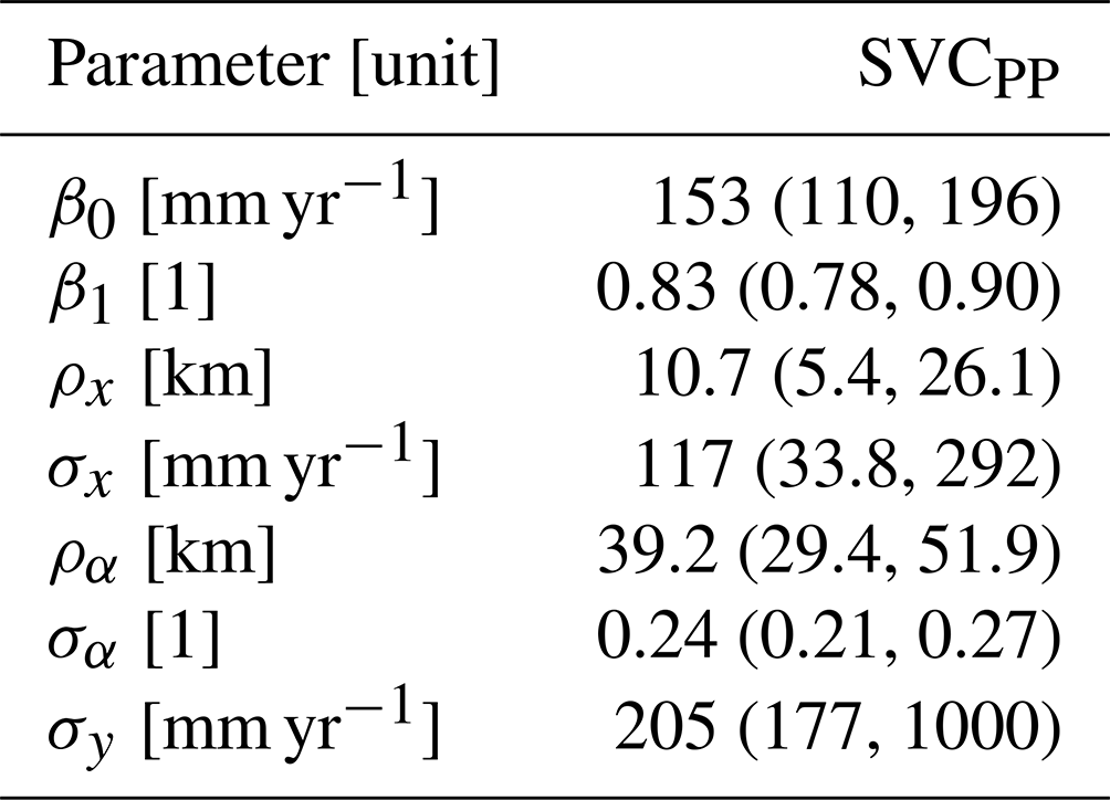
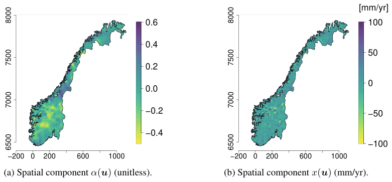
Figure 6Posterior means for the two GRFs x(u) and α(u) for SVCPP for the Norwegian mainland.
The covariate h(u) makes a large contribution to the final model with a regression coefficient β1 that is estimated to be 0.83. This can be seen in Table 1 where we present the parameter estimates of the SVC model. In Table 1 we also see that the marginal standard deviations σα and σx of the two spatial fields α(u) and x(u) are of considerable magnitude, confirming that there indeed is a regional trend in the fit between the original HBV product and the observed mean annual runoff. The regional trend can be studied in Fig. 6 where we show the two spatial fields α(u) and x(u). We see that the spatial pattern in Fig. 5a mostly originates from the SVC component α(u) for SVCPP (Fig. 6a). The other GRF x(u) contributes with more local adjustments in the mean annual runoff (Fig. 6b). The spatial fields have hence picked up both long-range and short-range processes.
The posterior standard deviation of the SVCPP in Fig. 5c shows that the uncertainty is decreased in areas where there are observations, particularly around the centroids of the gauged catchments. This is typical behavior for spatial models. In addition, the uncertainty follows the pattern we see in the original HBV map in Fig. 2a. The latter comes from the SVC component α(u)h(u), which allows for a variance that is inhomogeneous in space given the process-based product h(u). Figure 5c further shows that the SVC model gives relatively high posterior standard deviations in a small area in western Norway, south of Sognefjorden (around y-coordinate 6800). This can be explained by the fact that this is an area where we have few observations (see Fig. 1b) and also that the original HBV map performs poorly here.

Figure 7Scatter plot showing the predicted mean annual runoff for SVCPP and the observed mean annual runoff from fully gauged (orange) and partially gauged catchments (green).
In Fig. 7 we present a scatter plot that shows the fit between the runoff map in Fig. 5a and the observed catchment mean annual runoff. The results show that the SVCPP map corresponds considerably better to the observed runoff for the fully gauged catchments than in the original HBV map (Fig. 2b). The original HBV map gave a correlation of 0.933 between the predictions and the observations for the fully gauged catchments, while the corrected SVCPP map gives a correlation approximately equal to 1.
We also investigated the correlation between the map and the observed runoff for the partially gauged catchments where we only have 1–29 years of measurements in the 30-year period of interest (Fig. 7). For these catchments, the original HBV model gave an overall correlation of 0.917. The SVCPP map gives correlation 0.986. The correlations and Fig. 7 indicate that the SVCPP map provides a better fit for the partially gauged catchments than the original HBV map. Here, we cannot be entirely sure because the underlying observations from the partially gauged catchments in Fig. 7 are only approximations of the true runoff between 1981 and 2010, computed based on 1–29 annual observations from this period. It is, however, a positive sign that the fit for the partially gauged catchments (green) is not as good as for the fully gauged catchments (orange).
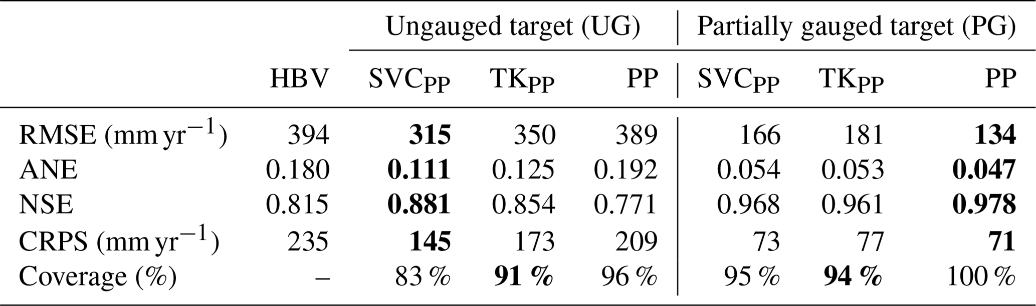
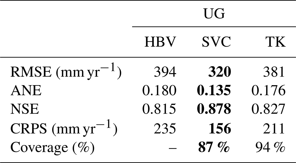
Table 2Predictive performance for the cross-validation experiments when the target catchments are treated as ungauged (UG) and partially gauged (PG) for the HBV model, the suggested SVC model, and for Top-Kriging (TK). Subscript PP refers to the geostatistical preprocessing step. The results from the geostatistical preprocessing method (PP) are also included as reference (without any further analysis) for a better understanding of the other results. The best method for each evaluation criterion is marked in bold.
6.2 Cross-validation for ungauged and partially gauged catchments
In Table 2 we present the results from the cross-validation assessment described in Sect. 5.2. For ungauged catchments (UG), we find that the RMSE of our SVCPP method is 20 % lower than the RMSE of the HBV model. Compared to TK, the SVCPP model gives 10 % lower RMSE. The ranking between the models is the same also for the ANE, NSE, and CRPS. When it comes to uncertainty quantification, TK gives the best uncertainty representation for ungauged catchments according to the 90 % coverage, with 91 % coverage. However, SVCPP also performs acceptably with 83 % coverage on a cross-validation performed on (only) 127 catchments.
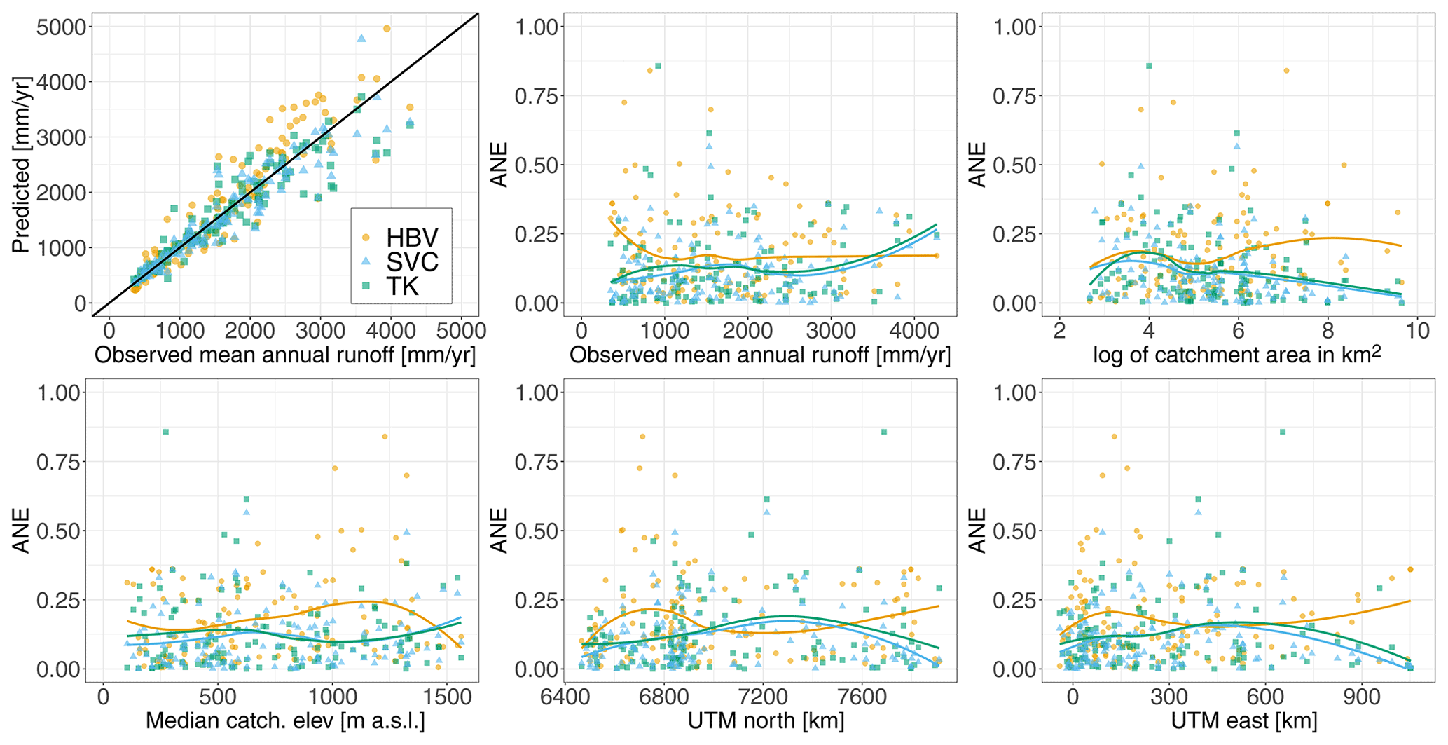
Figure 8Predictive performance of the methods (HBV, SVCPP, and TKPP) for predictions in ungauged catchments (UG) performed by cross-validation. The first plot shows the fit between the predictions and the observations for the methods. The remaining plots show the ANE for each of the 127 cross-validation catchments plotted against selected catchment attributes; i.e., the observed runoff, catchment area, median catchment elevation, UTM33 north, and UTM33 east. The fitted curves are regression splines (made by geom_smooth() in R).
In Table A1 in the Appendix, we include the methods' predictive performance for ungauged catchments when not using the preprocessing step and short records (SVC and TK). These results give the same ranking between the methods as before, but with one exception. SVC performs approximately as good as TK in terms of 90 % coverage, with coverages of 87 % and 94 %, respectively. From Table A1 we also notice that the difference in performance between the SVC model and TK is larger for this setting, where we had fewer observations. This is reasonable as we can expect the SVC model to be more robust than a purely data-driven model if the data availability is poorer.
Further, we compared the predictive performance for ungauged catchments (UG) for the SVCPP approach, the HBV model, and TK (TKPP) across the study area and across catchment attributes in terms of the ANE. The results are shown for selected catchment attributes in Fig. 8. We see that the HBV model in general tends to overestimate the mean annual runoff. It gives the highest ANE values in the southwestern part of the country, and particularly for catchments at higher elevations (800–1400 m a.s.l.). The latter might be due to the interpolated precipitation product used as input in the HBV model, where orographic enhancement of precipitation is accounted for by an elevation gradient. Since precipitation gauging stations are seldom located at high elevations (Lussana et al., 2018), the precipitation is extrapolated to the highest altitudes giving rise to biases in the precipitation field. Figure 8 further shows that the two geostatistical approaches (SVCPP and TKPP) perform better than the HBV model for catchments with mean elevations in the range 800–1400 m a.s.l. This demonstrates that the SVC approach is able to compensate for its poor HBV input in these areas.
The lines in Fig. 8 next show that TK and SVCPP in general tend to follow the same trends across catchment attributes. For example, both perform well for catchments with large drainage areas, supporting existing results from Viglione et al. (2013) regarding the predictive performance of TK. For catchments with large drainage areas, there are typically data from overlapping subcatchments available, which makes areal referenced geostatistical models particularly appropriate. The two geostatistical approaches also perform well for catchments located in the eastern parts of Norway. In southeastern Norway we find catchments with larger drainage areas and most of them are located at relatively low elevations. The data availability is also good in the southeastern parts of Norway, suitable for geostatistical modeling. It is hard to see a clear trend when SVCPP performs better than TK from Fig. 8, but we note that TK (and the HBV model) in general produces more extreme ANE values than the SVC model.
We next consider the performance of the models for predictions in partially gauged (PG) catchments. The results in Table 2 show that we obtain a large reduction in the predictive performance for the SVCPP, PG case compared to the case when we have no data from the target catchments (SVCPP, UG). The reduction in RMSE is 47 %. The improvement for SVCPP, PG compared to the HBV model is 58 %. Compared to TK, the SVCPP approach is slightly better in terms of RMSE, but approximately equally good in terms of ANE, NSE, CRPS, and 90 % coverage. Table 2 also shows that the TK estimates are substantially improved when including preprocessed short records from the target catchments in the likelihood (PG compared to UG for TKPP).
The improved performance of TKPP and SVCPP for the PG case is mainly caused by the preprocessing procedure's ability to perform (very) accurate predictions of Norwegian mean annual runoff when a few annual observations are available. In Table 2 we see that the input data provided by the preprocessing step (PP) alone give predictions that are better than the predictions of the SVCPP and TKPP approaches. The improved results for TKPP and SVCPP, however, show that the two geostatistical methods are able to exploit the good performance of PP, and that the SVC approach indeed can be used to combine both process-based data and data from fully gauged and partially gauged catchments.
We have presented a geostatistical model for mean annual runoff that incorporates simulations from a process-based model through an SVC and shown how short records can be included by using the methodology from Roksvåg et al. (2020) for filling in missing values.
In a preliminary study we tested models with only one spatial field, i.e., only x(u) or α(u) was included in Eq. (5). These models performed quite well in terms of both posterior mean and posterior uncertainty for the Norwegian dataset, which indicates that it might be satisfactory to use a model with only one spatial field for many study areas. However, our preliminary experiments also showed that a model with two spatial fields often gave a more realistic spatial distribution of uncertainty than a model with only one spatial field. Further, Fig. 6 showed that the model was able to capture both short- and long-range processes through its two fields, which can be a useful model property that can avoid excessive smoothing out of the process-based covariate by the model. In general, the importance of x(u) compared to α(u) depends on the study area, the data availability, and the quality of the process-based input model.
Table 2 shows that TKPP and SVCPP performed slightly poorer than the preprocessing input model alone for the partially gauged catchments (PG). When constructing the models, we did not want the SVC approach and TK to put too much weight on the more uncertain preprocessed short records. The latter was included in the model by specifying a larger (prior) observation uncertainty for the partially gauged catchments (0 %–23 % of the observed value) compared to the fully gauged catchments (0 %–6 % of the observed value). We have not tested how this uncertainty specification affects the results, but in future work, the SVCPP model and TKPP could be improved by selecting the observation uncertainty for the preprocessed data more carefully. The observation uncertainty for the partially gauged catchments can, e.g., be set independently of the fully gauged catchments and based on the record length of the short records. An option could also be to use the predictive uncertainty of the preprocessing method to specify the (prior) measurement uncertainty for the partially gauged catchments in the SVC model and TK.
In the paper, we presented a framework for estimating mean annual runoff, which is one of several key flow indices. The SVC framework can be used for other flow indices as well, but the computational complexity makes it most suitable for flow indices of longer temporal scale or for modeling long-term averages. In Eq. (7), we also assume a linear aggregation of runoff which is particularly appropriate for mass conservative variables like annual runoff. If the modeler wants to avoid this assumption, two simple model modifications are possible:
-
Make the runoff observations point referenced by letting Q(𝒜)=q(u𝒜) in Eq. (7), where u𝒜 is the centroid of catchment 𝒜 and q(⋅) is point runoff as defined in Eq. (5). This modification also enables inference on log-transformed data.
-
Add more covariates or random noise outside the integral in Eq. (7). This way the areal representation is preserved, but it becomes easier to violate the water balance constraints.
A potential weakness of the proposed model is that it consists of Gaussian components which can result in negative runoff estimates. Negative estimates can occur if the flow index and the corresponding study area have runoff observations close to 0. This is another argument for using the SVC model mainly for flow indices of a longer temporal scale. Negative predictions can also occur if the discretization of the study area and/or the SPDE mesh is too coarse relative to the spatial variability of the target variable. In the study presented here, no negative values were produced.
Figure 7 shows that the SVCPP gave a very good fit for the 127 fully gauged catchments, almost entirely reproducing the actual observed mean annual runoff in the resulting gridded map. We emphasize that the proposed method is not guaranteed to reproduce the observed value with the precision we saw in this case study. How good the fit is for the fully gauged catchments depends on the data quality, the gauging density, and the complexity of the spatial variability of the underlying hydrological process. Obtaining a correlation around 1 for the gauged catchments, as in Fig. 7, is not necessarily desirable either, as it might affect the fit for the ungauged catchments negatively. This might explain the over-confidence of the SVCPP model, expressed through the 83 % coverage for the UG case, in Table 2. It is possible to influence the model fit by making the prior observation uncertainty of wider or narrower.
In Norway the gauging density is moderate. We expect the suggested SVC model to outperform purely geostatistical methods such as TK for gauging densities that are low to moderate. For data-sparse areas, the process-based information provided by the HBV model is probably more important. This claim is based on intuition about the models under discussion, but is also indicated by our results. TK is closer to the SVC model in predictive performance for the dataset where we use data from 411 catchments (UG in Table 2) than for the reduced dataset where we only use data from 127 catchments (Table A1 in the Appendix).
Whether the suggested framework performs better than a purely geostatistical method is of course also connected to the quality of the process-based input model and the calibration procedures performed on it. However, our results have clearly demonstrated that it is possible to improve a process-based hydrological product by using the suggested framework. All experiments showed that the SVC approach improved the predictions compared to the original HBV simulations. The SVC model can hence be considered as an objective approach for correcting the simulations from a process-based model, and can reduce the need for subjective, manual corrections.
We have presented a Bayesian geostatistical model for annual runoff estimation that incorporates simulations from a process-based hydrological model through a covariate whose regression coefficient is allowed to vary in the study area according to a GRF. A preprocessing step for including short records was also suggested such that the model could exploit data from both fully gauged and partially gauged catchments.
The model was evaluated by estimating mean annual runoff for Norway (1981–2010), and simulations from the process-based HBV model were used as a covariate. The results showed that the suggested framework outperforms a purely process-based model when predicting runoff in ungauged and partially gauged catchments. The reduction in RMSE was 20 % for ungauged catchments and 58 % for partially gauged catchments. The increased predictive performance obtained compared to a purely process-based model is connected to the quality of the process-based product and the calibration procedures performed on it. However, all results show that the suggested framework is able to improve the predictions from a process-based model. The approach can hence be used as a objective method for correcting process-based runoff maps relative to data. The large reduction in RMSE for partially gauged catchments demonstrates that the preprocessing method from Roksvåg et al. (2020) can be incorporated into the proposed model to exploit short records.
The suggested model gave a 10 % lower RMSE than a purely geostatistical method (TK) when predicting runoff in ungauged catchments. Particularly if the gauging density is low to moderate, the suggested framework is expected to outperform purely geostatistical models. For catchments that had a few annual streamflow observations available, a purely geostatistical method performed equally well (TK) or slightly better (PP) than the proposed approach. Since most study areas consist of a mix of ungauged, fully gauged, and partially gauged catchments, the proposed SVC model stands out as a good approach for making a consistent gridded runoff map for a larger area.
We repeat the experiments from Sect. 5.1 and 5.2 for ungauged catchments, but we only use observations from the 127 fully gauged catchments in Fig. 1a. The runoff data from the partially gauged catchments are simply removed from the analysis. The experiments are included to show that the SVC model works regardless of preprocessing.
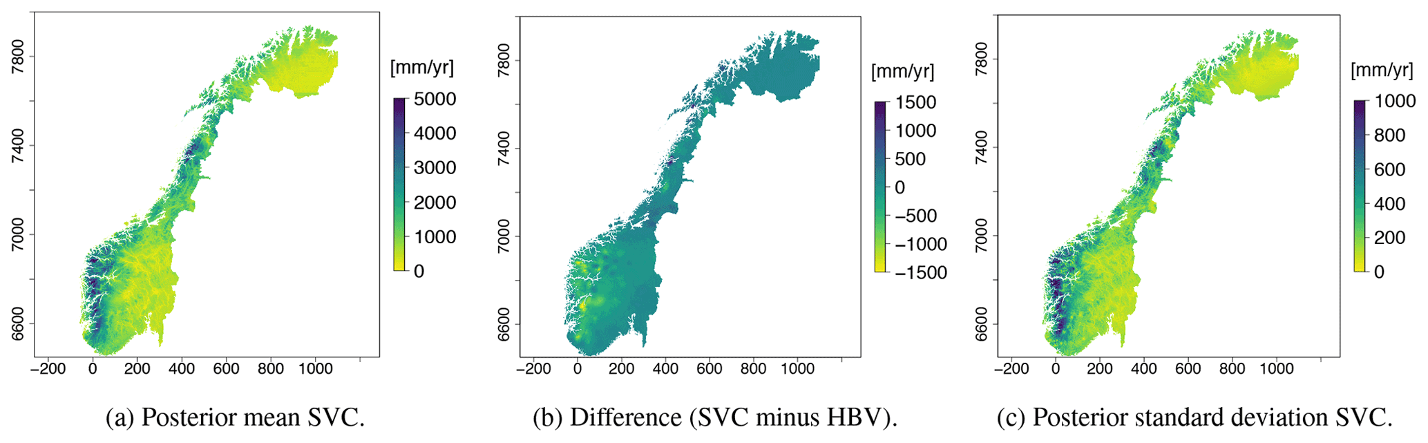
Figure A1Posterior mean of q(u) for all grid nodes, difference between the new map and the original HBV map, and posterior standard deviation of q(u). The model is fitted without including short records.
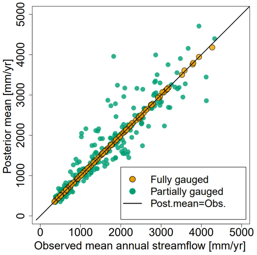
Figure A2Scatter plot showing the predicted mean annual runoff (posterior mean of Q(𝒜)) for SVC and the observed streamflow from fully gauged and partially gauged catchments when short records are omitted from the likelihood.
The runoff map provided by the SVC model, when not using short records, is shown in Fig. A1a. The maps look similar to the maps in Fig. 5a, but the posterior uncertainty is larger in western Norway in Fig. A1c. The reasons are that there are fewer observations available from western Norway in the dataset consisting only of fully gauged catchments and that this is an area with large deviance between the original HBV map and the observed streamflow.
In Fig. A2 we show the fit between the observed runoff and the runoff predicted by the map in Fig. A1a. The fit is good for the fully gauged catchments, as before. The fit is also improved for the partially gauged catchments compared to the original HBV map in Fig. 2a. Here, the original HBV model gave a correlation of 0.917 between observed and predicted values, while the map in Fig. A1a gives a correlation of 0.924. However, when short records and preprocessing were included in the analysis, the correlation was 0.986 (SVCPP in Fig. 7). This illustrates the reduced predictive performance when omitting short records from the analysis in Norway and in countries with similar spatiotemporal trends in annual runoff.
Table A1Predictive performance for cross-validation when the target catchments are treated as ungauged (UG) for the HBV model, the suggested SVC model, and for Top-Kriging (TK). Short records are omitted from the observation likelihood and the preprocessing step is not performed. The best method for each evaluation criterion is marked in bold.
The cross-validation results for the experiments where we omit the short records are summarized in Table A1. Again the SVC model performs considerably better than the HBV model and TK in terms of RMSE, ANE, NSE, and CRPS. Recall that the difference in performance from TK is larger for this dataset (for UG) compared to when using the larger dataset (Table 2).
The data and code used in this study can be provided by the main author upon request.
TR conducted the experiments, wrote the R code, wrote the majority of the paper, and created the figures. IS came up with the initial ideas and contributed with discussions throughout the work and with ideas for the experimental set-up. KE provided the data, contributed with discussions throughout the work, particularly regarding the HBV model, the data, and interpretation of the results, and wrote parts of Sect. 2.
The contact author has declared that none of the authors has any competing interests.
Publisher’s note: Copernicus Publications remains neutral with regard to jurisdictional claims in published maps and institutional affiliations.
We would like to thank Stein Beldring for providing the gridded HBV product and for valuable discussions around the work. We would also like to thank Erik Holmqvist for discussions about the data. Finally, we would like to thank Denis Allard and one anonymous reviewer for their contribution. Their insightful comments improved the quality of the final paper.
This research has been supported by the Norges Forskningsråd (grant no. 250362).
This paper was edited by Luis Samaniego and reviewed by Denis Allard and one anonymous referee.
Bakka, H., Rue, H., Fuglstad, G.-A., Riebler, A., Bolin, D., Illian, J., Krainski, E., Simpson, D., and Lindgren, F.: Spatial modeling with R-INLA: A review, WIREs Computational Statistics, 10, e1443, https://doi.org/10.1002/wics.1443, 2018. a
Banerjee, S., Gelfand, A., and Carlin, B.: Hierarchical Modeling and Analysis for Spatial Data, vol. 101 of Monographs on Statistics and Applied Probability, Chapman & Hall, ISBN 978-1584884101, 2003. a
Beldring, S., Roald, L. A., and Voksø, A.: Arenningskart for Norge. Årsmiddelverdier for avrenning 1961–1990, Tech. Rep. Oslo: NVE, ISSN 1501-2840, http://publikasjoner.nve.no/dokument/2002/dokument2002_02.pdf (last access: last access: 19 October 2022), 2002. a, b, c
Beldring, S., Engeland, K., Roald, L. A., Sælthun, N. R., and Voksø, A.: Estimation of parameters in a distributed precipitation-runoff model for Norway, Hydrol. Earth Syst. Sci., 7, 304–316, https://doi.org/10.5194/hess-7-304-2003, 2003. a
Bergström, S.: Development and Application of a Conceptual Runoff Model for Scandinavian Catchments, SMHI, Norrköping, Sweden, RHO 7, 134 pp., 1976. a, b
Blangiardo, M. and Cameletti, M.: Spatial and Spatio-temporal Bayesian Models with R-INLA, 1st edn., Wiley, ISBN 978-1-118-32655-8, 2015. a, b
Blöschl, G., Sivapalan, M., Wagener, T., Viglione, A., and Savenije, H.: Runoff Prediction in Ungauged Basins: Synthesis across Processes, Places and Scales, Camebridge University press, ISBN 978-1107028180, 2013. a, b, c, d
Borgvang, S., Stålnacke, P., Skarbøvik, E., Beldring, S., Selvik, J., Tjomsland, T., and Harsten, S.: Riverine inputs and direct discharges to Norwegian coastal waters –2004. OSPAR Commission for the Protection of the Marine Environment of the North-East Atlantic., Norwegian Institute for Water Research, Report no. 5135-2006, 159 pp., https://www.miljodirektoratet.no/globalassets/publikasjoner/klif2/publikasjoner/overvaking/2147/ta2147.pdf (last access: 19 October 2022), 2006. a
Brenner, S. and Scott, L.: The Mathematical Theory of Finite Element Methods, 3rd edn., vol. 15 of Texts in Applied Mathematics, Springer, ISBN 978-0-387-75934-0, 2008. a
Casella, G. and Berger, R.: Statistical Inference, Duxbury Press Belmont, ISBN 978-0534243128, 1990. a
Clark, M. P., Bierkens, M. F. P., Samaniego, L., Woods, R. A., Uijlenhoet, R., Bennett, K. E., Pauwels, V. R. N., Cai, X., Wood, A. W., and Peters-Lidard, C. D.: The evolution of process-based hydrologic models: historical challenges and the collective quest for physical realism, Hydrol. Earth Syst. Sci., 21, 3427–3440, https://doi.org/10.5194/hess-21-3427-2017, 2017. a
Cressie, N.: Statistics for spatial data, J. Wiley & Sons, ISBN 978-1119114611, 1993. a, b, c, d
Doherty, J.: PEST: Model Independent Parameter Estimation, Fifth edition of user manual, Watermark Numerical Computing, Brisbane, Australia, https://www.nrc.gov/docs/ML0923/ML092360221.pdf (last access 19.10.2022), 2004. a
Fatichi, S., Vivoni, E., Ogden, F., Ivanov, V., Mirus, B., Gochis, D., Downer, C., Camporese, M., Davison, J., Ebel, B., Jones, N., Kim, J., Mascaro, G., Niswonger, R., Restrepo, P., Rigon, R., Shen, C., Sulis, M., and Tarboton, D.: An overview of current applications, challenges, and future trends in distributed process-based models in hydrology, J. Hydrol., 537, 45–60, https://doi.org/10.1016/j.jhydrol.2016.03.026, 2016. a
Ferguson, C. A., Bowman, A. W., Scott, E. M., and Carvalho, L.: Multivariate varying-coefficient models for an ecological system, Environmetrics, 20, 460–476, https://doi.org/10.1002/env.945, 2009. a
Finley, A. O.: Comparing spatially-varying coefficients models for analysis of ecological data with non-stationary and anisotropic residual dependence, Methods Ecol. Evol., 2, 143–154, https://doi.org/10.1111/j.2041-210X.2010.00060.x, 2011. a
Fuglstad, G.-A., Simpson, D., Lindgren, F., and Rue, H.: Constructing Priors that Penalize the Complexity of Gaussian Random Fields, J. Am. Stat. Assoc., 114, 445–452, https://doi.org/10.1080/01621459.2017.1415907, 2019. a, b
Gamerman, D. and Lopes, H. F.: Markov chain Monte Carlo: stochastic simulation for Bayesian inference, Chapman and Hall/CRC, ISBN 9781584885870, 2006. a
Gamerman, D., Moreira, A., and Rue, H.: Space-varying regression models: specifications and simulation, Computational Statistics and Data Analysis, Computational Econometrics, 42, 513–533, https://doi.org/10.1016/S0167-9473(02)00211-6, 2003. a
Gelfand, A., Hyon-Jung, K., Sirmans, C., and Banerjee, S.: Spatial Modeling With Spatially Varying Coefficient Processes, J. Am. Stat. Assoc., 98, 387–396, https://doi.org/10.1198/016214503000170, 2003. a, b, c
Gelfand, A., Diggle, P., Fuentes, M., and Guttorp, P.: Handbook of Spatial Statistics, Chapman & Hall, 619 pp., https://doi.org/10.1201/9781420072884, 2010. a, b
Gelman, A., Carlin, J. B., Stern, H. S., and Rubin, D. B.: Bayesian Data Analysis, Chapman and Hall/CRC, 2nd edn., ISBN 978-1584883883, 2004. a
Gneiting, T. and Raftery, A. E.: Strictly Proper Scoring Rules, Prediction, and Estimation, J. Am. Stat. Assoc., 102, 359–378, https://doi.org/10.1198/016214506000001437, 2007. a
Guillot, G., Vitalis, R., le Rouzic, A., and Gautier, M.: Detecting correlation between allele frequencies and environmental variables as a signature of selection, A fast computational approach for genome-wide studies, Spatial Statistics, 8, 145–155, https://doi.org/10.1016/j.spasta.2013.08.001, 2014. a
Guttorp, P. and Gneiting, T.: Studies in the history of probability and statistics XLIX On the Matérn correlation family, Biometrika, 93, 989–995, https://doi.org/10.1093/biomet/93.4.989, 2006. a
Hanssen-Bauer, I., Førland, E. J., Haddeland, I., Hisdal, H., Mayer, S., Nesje, A., and Sorteberg, A.: Climate in Norway 2100 – a knowledge base for climate adaption, NCCS Report 1/2017, Retrieved from Oslo, Norway, https://www.miljodirektoratet.no/globalassets/publikasjoner/M741/M741.pdf (last access: 19 October 2022), 2017. a
Hastie, T. and Tibshirani, R.: Varying-Coefficient Models, J. Roy. Stat. Soc. B Met., 55, 757–779, https://doi.org/10.1111/j.2517-6161.1993.tb01939.x, 1993. a
Khan, D. and Warner, M.: A Bayesian spatial and temporal modeling approach to mapping geographic variation in mortality rates for subnational areas with r-inla, J. Data Sci., 18, 147–182, 2018. a
Laaha, G. and Blöschl, G.: Low flow estimates from short stream flow records – a comparison of methods, J. Hydrol., 306, 264–286, https://doi.org/10.1016/j.jhydrol.2004.09.012, 2005. a
Laaha, G., Skøien, J., Nobilis, F., and Blöschl, G.: Spatial Prediction of Stream Temperatures Using Top-Kriging with an External Drift, Environ. Model. Assess., 18, 671–683, 2013. a
Lawrence, D., Haddeland, I., and Langsholt, E.: Calibration of HBV hydrological models using PEST parameter estimation, Tech. Rep. Oslo: NVE, report no. 1, ISBN 978-82-410-0680-7, 2019. a
Lindgren, F., Rue, H., and Lindström, J.: An explicit link between Gaussian fields and Gaussian Markov random fields: the stochastic partial differential equation approach, J. Roy. Stat. Soc. B Stat. Met., 73, 423–498, https://doi.org/10.1111/j.1467-9868.2011.00777.x, 2011. a, b, c, d
Lindström, G., Johansson, B., Persson, M., Gardelin, M., and Bergström, M.: Development and test of the distributed HBV-96 hydrological model, J. Hydrol., 201, 272–288, https://doi.org/10.1016/S0022-1694(97)00041-3, 1997. a
Lu, Z., Steinskog, D. J., Tjøstheim, D., and Yao, Q.: Adaptively varying-coefficient spatiotemporal models, J. Roy. Stat. Soc. B Stat. Met., 71, 859–880, https://doi.org/10.1111/j.1467-9868.2009.00710.x, 2009. a
Lussana, C., Saloranta, T., Skaugen, T., Magnusson, J., Tveito, O. E., and Andersen, J.: seNorge2 daily precipitation, an observational gridded dataset over Norway from 1957 to the present day, Earth Syst. Sci. Data, 10, 235–249, https://doi.org/10.5194/essd-10-235-2018, 2018. a
Merz, R. and Blöschl, G.: Flood frequency regionalisation – Spatial proximity vs. catchment attributes, J. Hydrol., 302, 283–306, https://doi.org/10.1016/j.jhydrol.2004.07.018, 2005. a, b
Myrvoll-Nilsen, E., Sørbye, S. H., Fredriksen, H.-B., Rue, H., and Rypdal, M.: Statistical estimation of global surface temperature response to forcing under the assumption of temporal scaling, Earth Syst. Dynam., 11, 329–345, https://doi.org/10.5194/esd-11-329-2020, 2020. a
Opitz, T., Huser, R., Bakka, H., and Rue, H.: INLA goes extreme: Bayesian tail regression for the estimation of high spatio-temporal quantiles, Extremes, 21, 441–462, https://doi.org/10.1007/s10687-018-0324-x, 2018. a
Pannecoucke, L., Le Coz, M., Freulon, X., and de Fouquet, C.: Combining geostatistics and simulations of flow and transport to characterize contamination within the unsaturated zone, Sci. Total Environ., 699, 134216, https://doi.org/10.1016/j.scitotenv.2019.134216, 2020. a
Qiu, N., Chen, X., Hu, Q., Liu, J., Huang, R., and Gao, M.: Hydro-stochastic interpolation coupling with the Budyko approach for prediction of mean annual runoff, Hydrol. Earth Syst. Sci., 22, 2891–2901, https://doi.org/10.5194/hess-22-2891-2018, 2018. a
Roksvåg, T., Steinsland, I., and Engeland, K.: Estimation of annual runoff by exploiting long-term spatial patterns and short records within a geostatistical framework, Hydrol. Earth Syst. Sci., 24, 4109–4133, https://doi.org/10.5194/hess-24-4109-2020, 2020. a, b, c, d, e, f, g, h, i, j, k
Rue, H. and Held, L.: Gaussian Markov Random Fields: Theory and Applications, vol. 104 of Monographs on Statistics and Applied Probability, Chapman & Hall, London, ISBN 9781584884323, 2005. a
Rue, H., Martino, S., and Chopin, N.: Approximate Bayesian inference for latent Gaussian models using integrated nested Laplace approximations, J. Roy. Stat. Soc. B Stat. Met., 71, 319–392, https://doi.org/10.1111/j.1467-9868.2008.00700.x, 2009. a, b, c, d, e
Sauquet, E.: Mapping mean annual river discharges: geostatistical developments for incorporating river network dependencies, J. Hydrol., 331, 300–314, https://doi.org/10.1016/j.jhydrol.2006.05.018, 2006. a
Sauquet, E., Gottschalk, L., and Lebois, E.: Mapping average annual runoff: A hierarchical approach applying a stochastic interpolation scheme, Hydrol. Sci. J., 45, 799–815, https://doi.org/10.1080/02626660009492385, 2000. a, b
Simpson, D., Rue, H., Riebler, A., Martins, T. G., and Sørbye, S. H.: Penalising Model Component Complexity: A Principled, Practical Approach to Constructing Priors, Stat. Sci., 32, 1–28, https://doi.org/10.1214/16-STS576, 2017. a
Skarbøvik, E., Stålnacke, P., Kaste, ø., Selvik, J., Tjomsland, T., Høgåsen, T., Aakerøy, P., Haaland, S., and Beldring, S.: Riverine inputs and direct discharges to Norwegian coastal waters –2008, Norwegian Pollution Control Authority, Report no. TA-2569-2009, 75 pp., ISBN 978-82-577-5788-5, 2009. a
Skøien, J.O.: Package “rtop”, CRAN [software], https://cran.r-project.org/web/packages/rtop/rtop.pdf (last access: 25 October 2021), 2018. a
Skøien, J. O., Merz, R., and Blöschl, G.: Top-kriging – geostatistics on stream networks, Hydrol. Earth Syst. Sci., 10, 277–287, https://doi.org/10.5194/hess-10-277-2006, 2006. a, b, c
Sælthun, N.: The Nordic HBV model, Technical Report 07, Norwegian Water Resources and Energy Directorate, https://publikasjoner.nve.no/publication/1996/publication1996_07.pdf (last access: last access: 19 October 2022), 1996. a
Stein, M.: Interpolation of spatial data. Some theory for kriging, Springer series in statistics, Springer, New York, ISBN 978-1-4612-1494-6, 1999. a
Stohl, A., Forster, C., and Sodemann, H.: Remote sources of water vapor forming precipitation on the Norwegian west coast at 60∘ N – a tale of hurricanes and an atmospheric river, J. Geophys. Res.-Atmos., 113, D5, https://doi.org/10.1029/2007JD009006, 2008. a
Su, S., Lei, C., Li, A., Pi, J., and Cai, Z.: Coverage inequality and quality of volunteered geographic features in Chinese cities: Analyzing the associated local characteristics using geographically weighted regression, Appl. Geogr., 78, 78–93, https://doi.org/10.1016/j.apgeog.2016.11.002, 2017. a
Viglione, A., Parajka, J., Rogger, M., Salinas, J. L., Laaha, G., Sivapalan, M., and Blöschl, G.: Comparative assessment of predictions in ungauged basins – Part 3: Runoff signatures in Austria, Hydrol. Earth Syst. Sci., 17, 2263–2279, https://doi.org/10.5194/hess-17-2263-2013, 2013. a, b, c, d
Wang, Y., Akeju, O. V., and Zhao, T.: Interpolation of spatially varying but sparsely measured geo-data: A comparative study, Engin. Geol., 231, 200–217, https://doi.org/10.1016/j.enggeo.2017.10.019, 2017. a
Whittle, P.: On stationary processes in the plane, Biometrika, 41, 434–49, 1954. a
Whittle, P.: Stochastic processes in several dimensions, Bull. Int. Stat. Inst., 40, 974–994, 1963. a
WMO: International meteorological vocabulary, ISBN 978-92-63-02182-3, 1992. a
- Abstract
- Introduction
- Model input
- Methodological background
- An SVC model for incorporating process-based simulations and short records
- Experimental set-up and evaluation scores
- Results
- Discussion
- Conclusions
- Appendix A: Results when omitting short records
- Code and data availability
- Author contributions
- Competing interests
- Disclaimer
- Acknowledgements
- Financial support
- Review statement
- References