In situ estimation of soil hydraulic and hydrodispersive properties by inversion of electromagnetic induction measurements and soil hydrological modeling

Soil hydraulic and hydrodispersive properties are necessary for modeling water and solute fluxes in agricultural and environmental systems. Despite the major efforts in developing methods (e.g., laboratory-based, pedotransfer functions), their characterization at applicative scales remains an imperative requirement. Accordingly, this paper proposes a noninvasive in situ method integrating electromagnetic induction (EMI) and hydrological modeling to estimate soil hydraulic and transport properties at the plot scale. To this end, we carried out two sequential water infiltration and solute transport experiments and conducted time-lapse EMI surveys using a CMD Mini-Explorer to examine how well this methodology can be used to (i) monitor water content dynamic after irrigation and to estimate the soil hydraulic van Genuchten–Mualem parameters from the water infiltration experiment as well as (ii) to monitor solute concentration and to estimate solute dispersivity from the solute transport experiment. We then compared the results with those estimated by direct time domain reflectometry (TDR) and tensiometer probe measurements. The EMI significantly underestimated the water content distribution observed by TDR, but the water content evolved similarly over time. This introduced two main effects on soil hydraulic properties obtained by the two methods: (i) similar water retention curve shapes, but underestimated saturated water content from the EMI method, resulting in a scaled water retention curve when compared with the TDR method; the EMI-based water retention curve can be scaled by measuring the actual saturated water content at the end of the experiment with TDR probes or by weighing soil samples; (ii) almost overlapping hydraulic conductivity curves, as expected when considering that the shape of the hydraulic conductivity curve primarily reflects changes in water content over time. Nevertheless, EMI-based estimations of soil hydraulic properties and transport properties were found to be fairly accurate in comparison with those obtained from direct TDR measurements and tensiometer probe measurements.

1 Introduction

Dynamic agro-hydrological models are increasingly used for interpreting and solving agro-environmental problems (Hansen et al., 2012; Coppola et al., 2015, 2019; Kroes et al., 2017). The soil hydrological component of these models is frequently based on mechanistic descriptions of water and solute fluxes in soils. The Richards equation (RE) for water flow and the advection–dispersion equation (ADE) for solute transport are generally accepted for application at a local scale (plot scale, for example). Solving RE requires the determination of the hydraulic properties, namely, the water retention curve relating the soil water content, θ, to the soil water pressure head, h, and the hydraulic conductivity curve, relating the hydraulic conductivity K to either the water content θ or the pressure head h. Similarly, ADE requires the dispersivity, λ, to be also known. In the past few decades several laboratory and in situ methods have been developed for characterizing soil hydraulic properties (e.g., Dane and Topp, 2020) and dispersive properties (e.g., Vanderborght and Vereecken, 2007). Laboratory-based characterizations may be carried out under more controlled conditions. Nevertheless, for simulating water and solute dynamics in the real field context, the in situ methods are obviously more representative than laboratory methods. This is firstly related to the size of the volume investigated, which has to appropriately represent the heterogeneity of the medium being studied (Wessolek et al., 1994; Ellsworth et al., 1996; van Genuchten et al., 1999; Inoue et al., 2000). In fact, a water flow process observed in situ will be influenced by the heterogeneities (stones, macropores, etc.) found in the field. This is the main limitation of the relatively small soil columns generally analyzed in the laboratory. By contrast, an in situ characterization method, for example, the well-known instantaneous profile method (Watson, 1966), can capture the hydraulic properties which are effective in describing the flow process observed in situ. This will also depend on the measurement scale (the size of the plot) and on the observation scale of the sensors used. These issues have been dealt with in detail, for example, in Coppola et al. (2012, 2016) and in Dragonetti et al. (2018). Besides, the experimental boundary conditions used to carry out the hydraulic characterization in the laboratory and in situ may also induce a different shape of the hydraulic properties as determined in the laboratory and in situ (Basile et al., 2006).

In situ methods typically evaluate soil hydraulic properties by monitoring an infiltration and/or a redistribution water flow process (Watson, 1966). Similarly, in situ methods for determining hydrodispersive parameters are generally based on monitoring of mixing processes following pulse or step inputs of a tracer on either large plots or along a field transect (Severino et al., 2010; Coppola et al., 2011; Vanderborght and Vereecken, 2007). Inverse modeling is frequently used to estimate the hydraulic and transport parameters simultaneously (e.g. Šimůnek et al., 1998; Abbasi et al., 2003; Groh et al., 2018). Yet, even by shortening the measurement procedure through simplified assumptions (e.g. Sisson and van Genuchten, 1991; Basile et al., 2006) all in situ methods for the characterization of the whole soil profile remain extremely difficult to implement also because they generally require installing sensors at different depths (e.g., TDR probes, tensiometers, access tubes for neutron probe) which are cumbersome and may induce soil disturbance, unless the installation is made much earlier than the experiment, to at least partly allow the soil to recover through several wetting–drying cycles in its natural structure.

In this direction, geophysical noninvasive methods based on the electrical resistivity tomography (ERT) and electromagnetic induction (EMI) techniques represent a promising alternative to traditional sensors for assessment of soil hydraulic and transport parameters. Many researchers have used the time-lapse ERT data (e.g., Binley et al., 2002; Kemna et al., 2002; Singha and Gorelick, 2005) to monitor water content and saline tracers in the field. The dependence of soil electrical conductivity on soil water content and concentration is the key mechanism that enables the use of time-lapse ERT to monitor water and solute dynamics in a time-lapse mode along a soil profile, by relating resistivities to water content and solute concentration distributions through empirical or semi-empirical relationships (e.g., Archie, 1942) or established in situ relationships (e.g., Binley et al., 2002).

Electromagnetic induction (EMI) sensors may be also used as they make it possible to monitor water and solute propagation through a soil profile by simply moving the sensor above the soil surface without the need to install electrodes, as required by the ERT technique. An EMI sensor provides measurements of the depth-weighted apparent electrical conductivity (σ_a) according to the specific distribution of the bulk electrical conductivity (σ_b) as well as the depth response function of the sensor used (McNeill, 1980). The σ_a obtained from EMI sensors has been used to map the geospatial and temporal variability of the soil water content and salinity (Corwin and Lesch, 2005; Bouksila et al., 2012; Saeed et al., 2017). However, monitoring the propagation of the water and solutes with depth along a soil profile (as during a water infiltration or a solute transport experiment) requires the distribution of the σ_b with depth to be known over time, which can be obtained by inversion of the σ_a observations from the EMI sensor (see, e.g., Hendrickx et al., 2002; Lavoué et al., 2010; Deidda et al., 2014; von Hebel et al., 2014; Dragonetti et al., 2018; Moghadas, 2019; Farzamian et al., 2019a; Zare et al., 2020; McLachlan et al., 2020). More recently, this inversion has been facilitated by the development of multi-coil EM sensors which are designed to collect σ_a at multiple coil spacing and orientations simultaneously in one sensor reading. This enables a rapid investigation of the soil's electrical conductivity at several depth ranges in order to obtain soil water content (Huang et al., 2016; Whalley et al., 2017) and solute concentrations (Paz et al., 2020; Gómez Flores et al., 2022) quickly and cheaply. However, the potential of EMI sensors to assess soil hydraulic and hydrodispersive parameters has not been yet studied due to the lack of high-resolution and well-controlled experiments, which are required to capture the complexity of the water flow and transport process during infiltration experiments.

Figure 1 Schematic diagram of the proposed hydrogeophysical uncoupled approach.

According to these premises, in this paper we propose a procedure based on a sequence of water infiltration and solute transport experiments, both monitored by an EMI sensor, with the objective of estimating in situ the parameters of soil hydraulic properties and the dispersivity of a soil profile with a noninvasive EMI sensor and relatively short experiments at the plot scale. The sequence of water and solute infiltration has the main aim of discriminating the contribution of the water content and the soil solution electrical conductivity to the EMI-based σ_b. All the EMI data will be analyzed by a hydrological model within a so-called uncoupled framework. The goodness of the adopted approach will be evaluated by comparing the EMI-based hydraulic and hydrodispersive properties with those obtained from in situ TDR and tensiometer measurements. The aim is to explore an approach that does not need sensor installation and to minimize the data necessary for the in situ assessment of soil hydraulic and hydrodispersive properties.

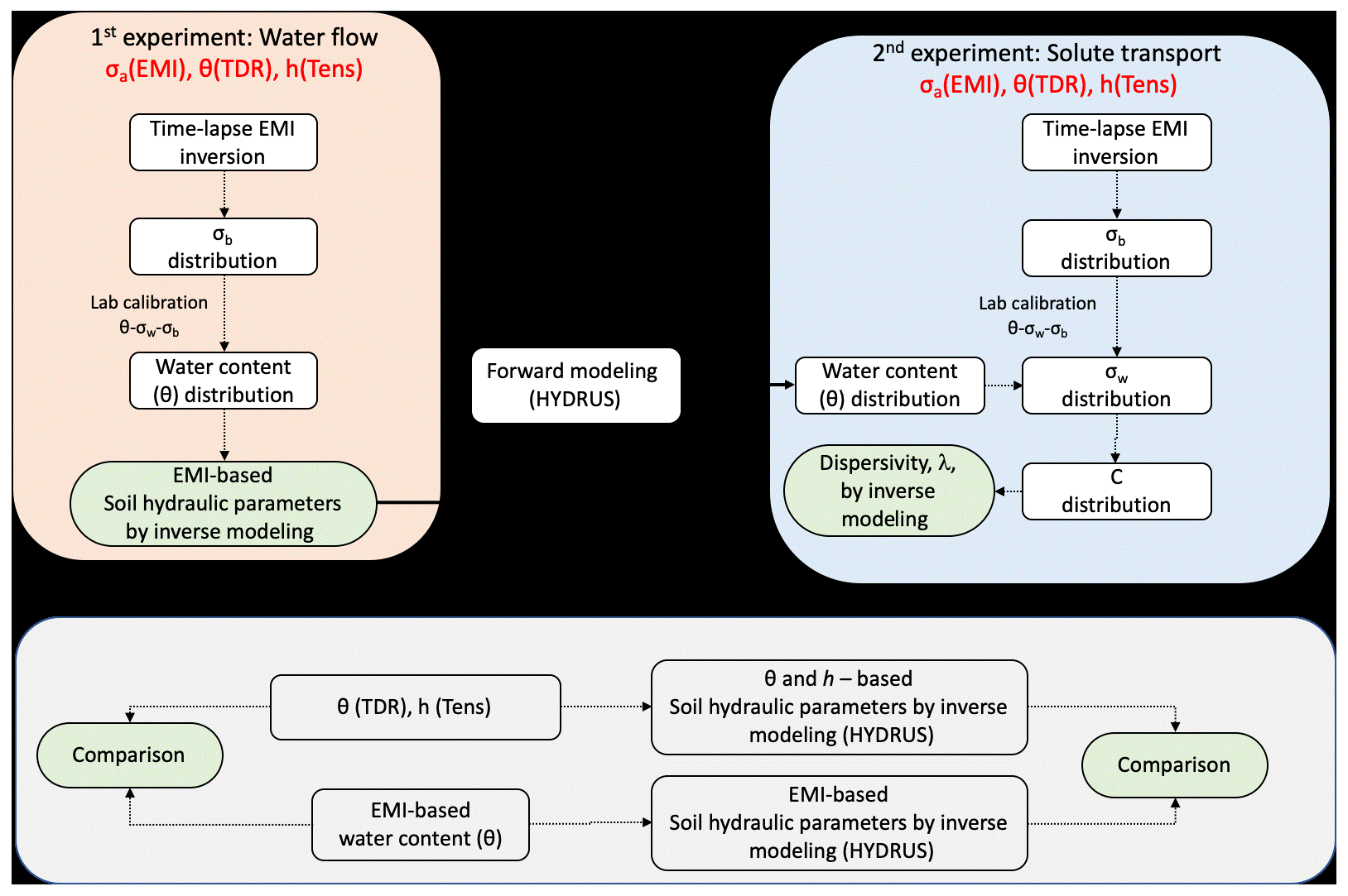
Figure 2 Layout of the experimental and monitoring set-up. HCP (horizontal coplanar) and VCP (vertical coplanar) are the vertical and horizontal dipolar orientations of the CMD probes, respectively.

2 Hydrogeophysical uncoupled approach

Figure 1 provides a schematic view of a six-step (+ one step for comparison) procedure, based on an uncoupled approach (Camporese et al., 2015) which will be adopted in this work to estimate the soil hydraulic and hydrodispersive properties using the data obtained from the EMI sensor. All the steps summarized below will be described in detail in Sect. 3.

• i.

  Inversion of time-lapse σ_a EMI data obtained during (i) a water infiltration experiment, hereafter “1st experiment”, and (ii) a subsequent solute transport experiment, hereafter “2nd experiment”, to generate EMI-based σ_b distributions for each experiment.

• ii.

  Laboratory calibration of the relationship θ–σ_b–σ_w in order to convert σ_b distributions to water content, θ, (1st experiment) and to soil solution electrical conductivity, σ_w, and therefore solute concentrations, C, (2nd experiment).

• iii.

  Converting the σ_b distributions obtained from the 1st experiment to water content distributions, using the θ–σ_b–σ_w relationship, to be used in the next numerical simulation step.

• iv.

  Numerical simulation, by using the HYDRUS-1D model (Šimůnek et al., 2013), of the 1st experiment in order to estimate the van Genuchten–Mualem (vG–M) parameters through an inversion procedure based on the water content inferred from step iii.

• v.

  Conversion of the σ_b distributions obtained from the 2nd experiment to solute concentration distribution in order to estimate longitudinal dispersivity, λ. In this step, σ_w distribution was estimated by using the laboratory θ–σ_b–σ_w calibration. The θ distribution in the 2nd experiment was simulated based on the vG–M parameters obtained in step iv. This is a crucial step in the proposed procedure, as it allows us to discriminate the contribution of the soil water electrical conductivity, and thus of the solute concentration, to the σ_b EMI readings during the 2nd experiment. The σ_w distributions were thus converted to solute concentration by a simple standard laboratory-based solute-specific σ_w–C relationship.

• vi.

  Numerical simulation of the second solute infiltration process in order to estimate λ through an inversion procedure based on the concentrations obtained from step v.

• vii.

  An alternative dataset of θ and σ_b obtained from direct TDR measurements, as well as tensiometer pressure head (h) readings, collected during the two experiments, allowed us to obtain independent hydraulic and hydrodispersive properties (hereafter “TDR-based” for the sake of simplicity) to be used as a reference to evaluate the EMI-based parameter estimation (see the horizontal gray box in Fig. 1).

3 Material and methods

3.1 Study area

The experiment was performed at the Mediterranean Agronomic Institute of Bari (CIHEAM-IAM), southeastern coast of Italy. The study area is located at an altitude of 72 m with 41^∘3^′13.251^′′ N, a longitude of 16^∘52^′36.274^′′ E, with a typical Mediterranean climate with rainy winters and very hot dry summers. The soil is a Colluvic Regosol consisting of silty loam layers of an average depth of 70 cm on a shallow fractured calcareous rock. Two main horizons on the calcareous rock may be identified: an Ap horizon (depth 0–30 cm) and a Bw horizon (depth 30–70 cm). Scattered calcareous fragments are present due to the breaking and grinding of the bedrock in the past through the use of heavy machinery to improve the soil structure and increase the soil depth for plantation.

3.2 Experimental set-up

A layout of the experimental setup is shown in Fig. 2. The plot size is 4×4 m. Water was applied by using a drip irrigation system consisting of 20 lines, with drippers spaced at 0.20 m and delivering a nominal flow rate of 10 L h⁻¹. Thus 400 drippers were installed, capable of delivering 4000 L h⁻¹ over the whole plot. The dripper's grid spacing and the flow rate were selected to ensure that a 1D flow field rapidly developed after starting irrigation. The drip irrigation system was placed on a metallic grid to be easily removed from the plot and whenever EMI measurements were taken on the ground soil.

Several months before starting the 1st experiment, after digging a small pit, eight three-wire TDR probes, 7 cm long, 2.5 cm internal distance, and 0.3 cm in diameter, were inserted horizontally at two depths – 20 and 40 cm, corresponding to the Ap and the Bw horizon – in the four corners of the experimental plot (at 1 m distance from the plot edge), as shown in Fig. 2. The pits for installing the sensors were refilled immediately to leave some natural wetting and drying cycles in order to reproduce the original soil aggregation. Then, the plot was covered with a plastic sheet about 4 d prior to the start of the experiment to keep the plot under quasi-equilibrium conditions at the beginning of the experiment.

A Tektronix 1502C cable tester (Tektronix Inc., Baverton, OR) was used in this study, enabling simultaneous measurement of water content, θ, and bulk electrical conductivity, σ_b, of the soil volume explored by the probe (Robinson et al., 2003; Coppola et al., 2011, 2013). Furthermore, eight tensiometers were vertically inserted near each TDR probe to acquire water potentials by a Tensicorder sensor (Hydrosense3 SK800). Both TDR probes and tensiometers were installed for the evaluation of the EMI-based parameter estimation (step vii).

The experimental plot was firstly irrigated by using tap water with an electrical conductivity of about 1 dS m⁻¹ (1st experiment). We applied 11 irrigations, each lasting about 3 min to deliver approx. 180 L over the whole 16 m² plot for each irrigation (the volume was measured by a flowmeter). Irrigations were separated by a shutoff of about 1 h. At each irrigation start, due to the short inertia of the irrigation system just after switching it on, for some seconds drippers delivered less than 10 L h⁻¹. For each irrigation an average flow rate of about 0.375 cm min⁻¹ was applied, which generated a small ponding at the soil surface for a short time. Overall, an average water volume of 2000 L was supplied.

The propagation of the wetting front along the soil profile was monitored by using an EMI sensor (i.e., CMD Mini-Explorer, GF Instruments, Czech Republic), positioned horizontally in the middle of the plot (Fig. 2) in order to measure the apparent electrical conductivity, σ_a, in the soil profile in VCP (vertical coplanar, i.e., horizontal magnetic dipole configuration) mode and then HCP (horizontal coplanar, i.e., vertical magnetic dipole configurations) mode by rotating the probe 90^∘ axially to change the orientation from VCP to HCP mode. The CMD Mini-Explorer operates at 30 kHz frequency and has three receiver coils with 0.32, 0.71, and 1.18 m distances from the transmitter coil, referred to hereafter as “ρ3 2”, “ρ71”, and “ρ118”. The manufacturer indicates that the instrument has an effective depth range of 0.5, 1.0, and 1.8 m in the HCP mode, which is reduced to half (0.25, 0.5, and 0.9 m) by using the VCP orientation. As a consequence, this EMI sensor returns six different σ_a values (utilizing three offsets with two coil orientations) with each corresponding to different depth sensitivity ranges. All measurements were performed 5 min after each water pulse application by temporarily removing the irrigation grid and placing the EMI sensor in the middle of the plot. The infiltration was also monitored by TDR probes and tensiometers in order to monitor the space–time evolution of water content, θ, pressure head, and h as well as the bulk electrical conductivity, σ_b. The distance of the TDR probes and tensiometers to the middle of the plot was specifically designed to avoid any interference with the EMI measurements.

At the end of the 1st experiment, the soil was allowed to dry and then covered with a plastic sheet to bring the distribution of water content along the profile similar to the initial one (observed before the water infiltration test). Afterward, a similar infiltration experiment (2nd) was carried out but using saline water this time at an electrical conductivity of 15 dS m⁻¹, and obtained by mixing CaCl₂ into the tap water. Again, 11 saline water supplies were provided at intervals of about 1 h apart and a total volume of 2000 L saline water was supplied during the experiment. The propagation of the water and chloride during the 2nd infiltration experiment was monitored similarly to the 1st experiment using TDR probes, tensiometers, and the CMD Mini-Explorer sensor.

3.3 Site-specific calibration θ–σ_b–σ_w

The relationship between the bulk electrical conductivity (σ_b), the electrical conductivity of the soil solution soil water (σ_w), and the water content was obtained by using the model proposed by Malicki and Walczak (1999):

$$\begin{array}{}\text{(1)}& {\mathit{\sigma }}_{\mathrm{w}}={\displaystyle \frac{{\mathit{\sigma }}_{\mathrm{b}}-a}{\left({\mathit{\epsilon }}_{\mathrm{b}}-b\right)(\mathrm{0.0057}+\mathrm{0.000071}S),}}\end{array}$$

where ε_b (–) is the dielectric constant, which is related to the water content, and S is the sand content in percent. The parameters a=3.6 dS m⁻¹, and b=0.11 were obtained in a laboratory experiment reported by Farzamian et al. (2021). Topp's equation was used to relate thw dielectric constant to the volumetric water content (Topp et al., 1980). The laboratory experiment for such a calibration is quite simple, fast, and standard procedure on reconstructed soil samples. An additional linear calibration, obtained by using solutions at different concentrations of calcium chloride, was used to relate soil water concentrations of chloride, Cl⁻, to σ_w.

3.4 Inversion of time-lapse EMI σ_a data

Time-lapse σ_a data obtained during the experiments were inverted using a modified inversion algorithm proposed by Monteiro Santos (2004) to obtain σ_b distribution in time. The aim of the inversion is to minimize the penalty function that consists of a combination between the observation misfit and the model roughness (Farzamian et al., 2019b). The earth model used in the inversion process consists of a set of 1D models distributed according to the number of time-lapse measurements. All the models have the same number of layers (i.e., 7) whose thickness is kept constant. The selected depths of layers are 10, 20, 30, 40, 55, 75, and 180 cm. The number and thickness of layers were selected based on several factors including the number of σ_a measurements (i.e., 6), effective depth range of HCP and VCP modes (i.e., 5 of 6 measurements have an effective depth of less than 1 m), and site specifications (i.e., the large variability of conductivity of the soil profile over a resistive bedrock). The parameters of each model are spatially and temporally constrained using their neighbors through smooth conditions. The forward modeling is solved based on the full solution of the Maxwell equations (Kaufman and Keller, 1983) to calculate the σ_a responses of the model. The inversion algorithm is Occam-regularization and the objective function was developed based on Sasaki (2001). Therefore, the update of the parameters in an iterative process is calculated solving the system

$$\begin{array}{}\text{(2)}& \left[\left({\mathbf{J}}^{T}J+\mathit{\eta }{\mathbf{C}}^{T}C\right)\right]\mathit{\delta }\mathit{p}={\mathbf{J}}^T\mathit{b},\end{array}$$

where δp is the vector containing the corrections applied to the parameters (logarithm of block conductivities, p_j) of an initial model, b is the vector of the differences between the logarithm of the observed and calculated ${\mathit{\sigma }}_{\mathrm{a}}[b_i=\ln ({\mathit{\sigma }}_{\mathrm{a}}^o/{\mathit{\sigma }}_{\mathrm{a}}^c{)}_i$], J is the Jacobian matrix whose elements are given by (${\mathit{\sigma }}_j/{\mathit{\sigma }}_{{\mathrm{a}}_i}^c$) ($\partial {\mathit{\sigma }}_{a_i}^c\partial {\mathit{\sigma }}_j$), the superscript T denotes the transpose operation, and η is a Lagrange multiplier that controls the amplitude of the parameter corrections and whose best value is determined empirically. The elements of matrix C are the coefficients of the values of the roughness of each 1D model, which is defined in terms of the two neighbor's parameters and the constraint between the parameters of the different models on time. In this regard and in the temporal 1D experiment, each cell is constrained spatially by its vertical neighbors, while the temporal constraints are imposed using its lateral neighbors. An iterative process allows the final models to be obtained, with their response fitting the dataset in a least-square sense. In terms of η, generally, large values will produce smooth inversion results with smoother spatial and temporal variations.

We performed several synthetic tests to determine how well the proposed inversion algorithm can predict the spatiotemporal variability of σ_b and to fine-tune the regularization parameters. The synthetic scenarios were selected based on spatiotemporal variability of σ_a in the HCP and VCP modes, the site specification (e.g., shallow bedrock), and the expected evolution of conductive zone due to water and saline water infiltrations.

3.5 Numerical simulation of water flow and chloride transport in soil

The water and the chloride propagations monitored during the experiments were simulated by using the HYDRUS-1D model (Šimůnek et al., 2013). HYDRUS-1D simulates water flow and solute transport by solving the Richards equation and the advection–dispersion equation, respectively.

The Richards equation can be written for 1D, unsaturated, non-steady-state flow of water in the vertical direction as follows:

$$\begin{array}{}\text{(3)}& C_{\mathrm{w}}\left(\mathit{\theta }\right){\displaystyle \frac{\partial h}{\partial t}}={\displaystyle \frac{\partial }{\partial Z}}\left[K\left(h\right){\displaystyle \frac{\partial h}{\partial Z}}+K\left(h\right)\right],\end{array}$$

where C_w(θ), the water capacity, is the slope of the water retention curve, θ is the volumetric water content [L³ L⁻³], h is the soil water pressure head [L], and K(h) is the unsaturated hydraulic conductivity [L T⁻¹].

The advection–dispersion equation governing the transport of a single nonreactive and nonadsorbed (a tracer, chloride in this case) ion in the soil can be written as

$$\begin{array}{}\text{(4)}& {\displaystyle \frac{\partial \left(\mathit{\theta }C\right)}{\partial t}}={\displaystyle \frac{\partial }{\partial z}}\left[\mathit{\theta }D{\displaystyle \frac{\partial C}{\partial z}}-qC\right],\end{array}$$

where q is the Darcian flux, C is the solute concentration in the liquid phase [M L⁻³] and D (L² T⁻¹) is the effective dispersion coefficient, which can be assumed to come from a combination of the molecular diffusion coefficient, D_diff (L² T⁻¹) and the hydrodynamic dispersion coefficient, D_dis (L² T⁻¹),

$$\begin{array}{}\text{(5)}& D=D_{\mathrm{diff}}+D_{\mathrm{dis}},\end{array}$$

where hydrodynamic dispersion is the mixing or spreading of the solute during transport due to differences in velocities within a pore and between pores. The dispersion coefficient can be related to the average pore water velocity $v=q/\mathit{\theta }$ through

$$\begin{array}{}\text{(6)}& D=\mathit{\lambda }v,\end{array}$$

where λ [L] is the dispersivity, a characteristic property of the porous medium. To solve the Richards equation (Eq. 3), the water retention function, θ(h), and the hydraulic conductivity function, K(h), must be defined. In this paper we adopted the van Genuchten–Mualem model (vG–M), (van Genuchten, 1980):

$$\begin{array}{}\text{(7)}& {\displaystyle }& {\displaystyle }{S}_{\mathrm{e}}=[\mathrm{1}+(\mathit{\alpha }\left|h\right|{)}^n{]}^{-m}\text{(8)}& {\displaystyle }& {\displaystyle }K\left(h\right)=K_{\mathrm{s}}{S}_{\mathrm{e}}^{\mathit{\tau }}{\left[\mathrm{1}-{\left(\mathrm{1}-S_e^{\mathrm{1}/m}\right)}^m\right]}^{\mathrm{2}}.\end{array}$$

In Eqs. (7) and (8), $S_{\mathrm{e}}=\frac{\left(\mathit{\theta }-{\mathit{\theta }}_{\mathrm{r}}\right)}{\left({\mathit{\theta }}_{\mathrm{s}}-{\mathit{\theta }}_{\mathrm{r}}\right)}$ is the effective water saturation, θ_s the saturated water content, θ_r the residual water content, α, n, and m are fitting parameters with m taken as $m=\mathrm{1}-\mathrm{1}/n$, K_s is the saturated hydraulic conductivity, and τ is the pore-connectivity parameter.

3.6 Inverse estimation of soil hydraulic and solute transport parameters

The obtained EMI-based spatiotemporal distribution of σ_b during the 1st experiment was converted to the θ distribution in order to estimate the temporal evolution of θ during the infiltration process. These water content data were then used in an optimization procedure with the HYDRUS-1D model in order to estimate the hydraulic properties of the different horizons in the soil profile. The simulations were carried out by using the actual top boundary flux conditions during the experiment, including the irrigation events. For the bottom boundary, free drainage was considered. A simulation domain of 150 cm depth was considered. The same procedure was repeated using the direct measurements of θ and h inferred from TDR and tensiometers, respectively, in order to obtain independent hydraulic parameters (TDR-based estimation) to be compared with those inferred from EMI. A three-layer soil profile (0–25; 25–70; 70–150 cm), reflecting the actual pedological layering (i.e., Ap, Bw, and bedrock) was used in all simulations. In terms of the initial condition, a hydrostatic distribution of the pressure heads, h, was considered for the TDR-based simulations. On the other hand, the water content distribution, inferred from the first EMI survey (before irrigation) was considered for the EMI-based simulation.

As for the solute transport experiment, a HYDRUS-1D simulation was carried out with the EMI-based hydraulic properties obtained from the 1st experiment to simulate the water content distributions corresponding to the EMI measurement times. The simulations of water infiltration and solute transport in the 2nd experiment were carried out by using the top boundary fluxes conditions applied during the 2nd experiment along with the same simulation domain, the three-layer soil profile, and the bottom boundary and equilibrium initial conditions described above. Thus, for each monitoring time, we had available the σ_b distributions obtained from the EMI and the θ distributions from the HYDRUS-1D simulations. These distributions allowed us to estimate as many σ_w (and thus C) as σ_b distributions by using the q–σ_b–σ_w relationship obtained in the laboratory. These C distributions were used in a new HYDRUS-1D simulation to estimate the longitudinal dispersivity of the investigated soil. The simulated concentrations, with the optimized dispersivity, λ, were compared with those obtained from the TDR and tensiometer data.

4 Results and discussion

4.1 Water infiltration – 1st experiment

4.1.1 Time-lapse σ_a data and estimation of σ_b distribution

Figure 3 shows the σ_a values observed during the water infiltration experiment. Both VCP and HCP modes show a relatively similar pattern of σ_a values with ρ32 and ρ118 being the highest and lowest, respectively. The HCP mode shows higher values than the VCP mode in the same receivers. This pattern of σ_a distribution suggests the presence of a conductive zone over a resistive zone, which is expected in this experiment as a result of the waterfront being infiltrated into the soil profile and the presence of a resistive bedrock. In terms of temporal σ_a variabilities, the σ_a increases consistently in both VCP and HCP modes during the first 3 h of the experiment. Afterward, σ_a did not change significantly toward the end of the experiment. The range of σ_a variations is relatively small in both VCP and HCP modes with the former in the 10–30 mS m⁻¹ range and the latter in the 10–50 mS m⁻¹ range.

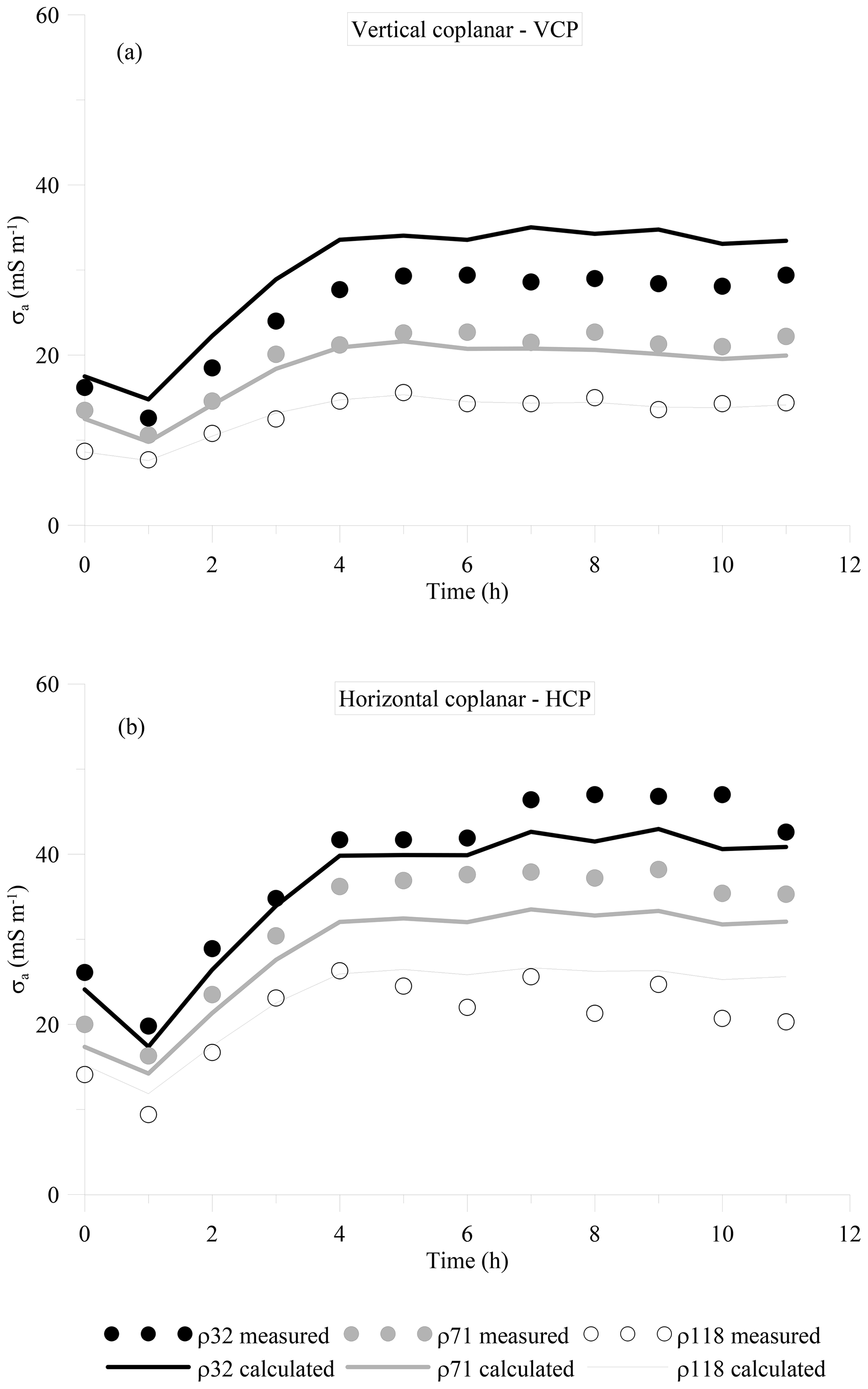
Figure 3 Values of σ_a observed during the water infiltration experiment. (a) VCP, (b) HCP. The symbols represent the measured data whereas the lines represent the values calculated after the inversion.

Prior to the inversion of σ_a data, we fine-tuned the regularization parameter, η, as discussed in Sect. 3.4. The results of several synthetic tests (not shown here) suggest that a value of η between 1 and 5 provides a better result in resolving the spatiotemporal σ_b distributions in both experiments. Figure 4 depicts the time-lapse σ_b modeling results of σ_a shown in Fig. 3. The model shows clearly the evolution of the conductive zone into the soil profile shortly after the irrigation started as expected from the σ_a data. The resistive zone beneath a conductive zone corresponds to the bedrock layer in the experimental plot. The σ_b of the resistive zone remains below 5 mS m⁻¹ and does not vary significantly during the experiment, while, by contrast, the σ_b of the upper layers increased significantly from an average of 20 mS m⁻¹ at the beginning of the experiment to more than 50 mS m⁻¹ after the fifth irrigation. The conductivity of this zone does not increase largely since then, suggesting that the upper soil is fairly saturated after the fifth irrigation. The calculated response of this model is shown in Fig. 3. There is a fairly good agreement between σ_a measurements and model response; however, a slight shift can be noticed in the ρ32-VCP mode and ρ71-HCP mode between the data and model response. This shift can be due to several reasons such as (i) the instrumental drift of the EMI sensor, (ii) the large spatiotemporal variability of soil electrical conductivity in this experiment as well as the smoothness constraint performed in the inversion process to stabilize the inversion process, which makes it difficult to resolve the sharp changes, and (iii) the choice of initial model.

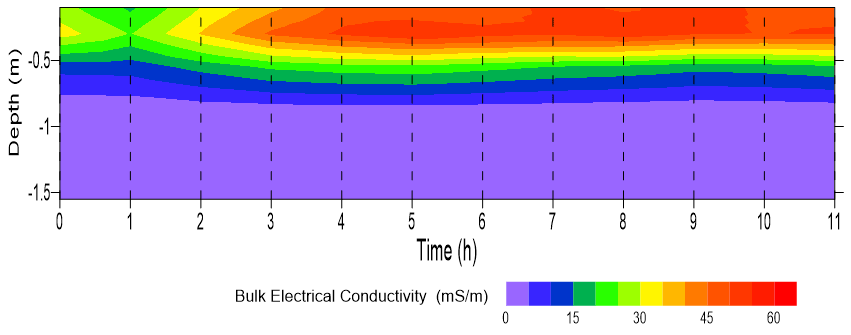
Figure 4 Time evolution of bulk electrical conductivity (σ_b) distribution with depth during the water infiltration experiment.

4.1.2 Comparison between TDR-based and EMI-based σ_b and θ distributions

Figure 5 shows the temporal σ_b changes inferred from TDR and EMI observations at two depths: 20 and 40 cm. As reported by some authors (e.g., Coppola et al., 2016; Dragonetti et al., 2018), both techniques provide σ_b estimations but a direct comparison between σ_b by TDR and EMI is not straightforward due to different observation volumes of the two sensors. However, this comparison can be used as a means to investigate the consistency of the σ_b trends and to provide an insight into the uncertainty associated with the EMI survey and inversion process in resolving the water infiltration process into the soil profile. Note that the average of TDR measurements in four corners at depths of 20 and 40 cm were considered both in this comparison and in the inversion procedure. The average values and the standard deviation of TDR measurements are presented in Fig. 5.

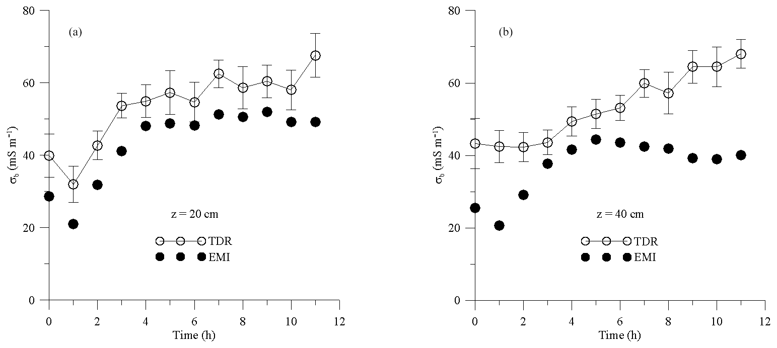
Figure 5 Evolution of σ_b as estimated from the TDR and EMI measurements at 20 cm (a) and 40 cm (b) depths. The vertical bars represent the standard deviation of the measurements obtained by the four TDR sensors.

Focusing on the σ_b series inferred from both TDR observations and EMI inversion, a similar time pattern of σ_b variability is evident, but in general, the EMI model underestimates the σ_b obtained by TDR. A better agreement was observed at 20 cm in terms of both absolute σ_b values and trend (r=0.94; mean error = 10.1 mS m⁻¹). By contrast, at 40 cm, the mismatch between TDR observations and EMI inversions becomes larger at the end of the experiment. The EMI σ_b values – especially at 40 cm depth – remain relatively invariant in the last part of the infiltration experiment. The general outcome that for both layers the EMI σ_b values underestimate the TDR σ_b measurements has been frequently reported in the literature (e.g., von Hebel et al., 2014; Coppola et al., 2015; Dragonetti et al., 2018; Visconti and de Paz, 2021). Furthermore, TDR measurements show a low local variability, which is depicted in Fig. 5 by the error bars reporting the standard deviation of the σ_b as measured by the four TDR probes.

Figure 6 shows the evolution of θ at the same two depths, 20 and 40 cm, as observed by TDR and EMI sensors. TDR provides the direct in situ measurement of θ. By contrast, in order to estimate θ from EMI observation, σ_b values extracted at these depths (Fig. 4) were converted to θ by the calibration performed in the laboratory, as detailed in Farzamian et al. (2021). A rapid increase of θ is visible shortly after injection in both EMI-based and TDR-based measurements. The EMI-based θ estimation is able to detect the similar water content evolution (similar water content differences over time) observed by TDR measurements but at a different water content level. Specifically, EMI water content was lower than that of TDR but the two series showed a quasi-parallel evolution at 20 cm depth (r=0.98; mean error = 0.09 cm³ cm⁻³), while diverging for longer times at 40 cm depth (r=0.60; mean error = 0.17 cm³ cm⁻³).

Figure 6 Evolution of θ measured by TDR (circles) and estimated from EMI measurements (triangles) at 20 cm (a) and 40 cm (b) depths. Continuous lines for TDR and dashed lines for EMI refer to the estimation obtained by the inversion procedure of the water infiltration process (see Sect. 4.1.3).

4.1.3 Estimation of hydraulic properties

In order to estimate the parameters of the hydraulic properties, an inversion procedure was carried out applying HYDRUS-1D. The first set of hydraulic parameters was obtained by using the soil water content measured by TDR and the pressure heads measured by tensiometers as measured data in the objective function for the optimization procedure (TDR-based). The second set of hydraulic parameters was obtained by using the soil water content estimated by EMI measurements as measured data (EMI-based). The inversion simulations were carried out by fixing θ_r=0 and τ=0.5, while θ_s, α, n, and K_s were optimized for both the Ap and the Bw layers. The hydraulic properties of the bedrock were already known and fixed to θ_r=0.068, θ_s=0.354, α=0.055, n=3.67, τ=0.5, and K_s=19.02 according to Caputo et al.(2010, 2015). We want to stress here that an a priori characterization of the bedrock layer is not essential and the proposed procedure holds independently of the presence of bedrock. We could have treated the bedrock layer like any other layer in the soil profile, but inserting TDR probes and tensiometers into bedrock presents difficulties. Therefore, we decided to fix the bedrock parameters to the values already available from independent measurements. In different soils with either deeper or absent bedrock, we could have inserted TDR probes into deeper layers of the profile and applied the procedure to any of them.

In the inversion procedure, the parameters were determined separately for each horizon of the profile (Abbaspour et al., 1999). First, the parameters for the topsoil were estimated and these parameters were then treated as known for the second layer estimation. Although the water content development in one layer is not independent of the hydraulic properties of the other layers when long-time evolution is considered, in the case of a relatively short infiltration event, as used here, this approach makes parameter estimation of multi-layered profiles feasible. It should be noted that in the case of the TDR-based estimations, optimization involved both measured water content and pressure head data, whereas the EMI-based estimations only involved “measured” water content.

Figure 6 reports a comparison between water content measured (symbols) and estimated (lines) by the inversion procedure. The θ evolution was properly estimated at 20 cm depth in both approaches. It is worth noting here that, despite the differences in the absolute value of the water content, a clearly parallel behavior of the two curves was observed, suggesting similar water content changes over time. A lower agreement was obtained at 40 cm but still reproduced similar water content changes over time. This is a crucial point in this paper, as the parallel behavior of the water content evolution will explain the similar shape of hydraulic properties we found for the TDR- and EMI-based estimations (see Fig. 8).

Similarly, in Fig. 7 the measured (points) and estimated (lines) values of pressure heads are shown. The simulated values of pressure head closely follow the measured value (r=0.950 at 20 cm and r=0.986 at 40 cm depth). Furthermore, the error bars, reporting the standard deviation of the pressure head as measured by the four tensiometers, overlap when the profile is wet (i.e., after the sixth irrigation) and separate during the wetting process.

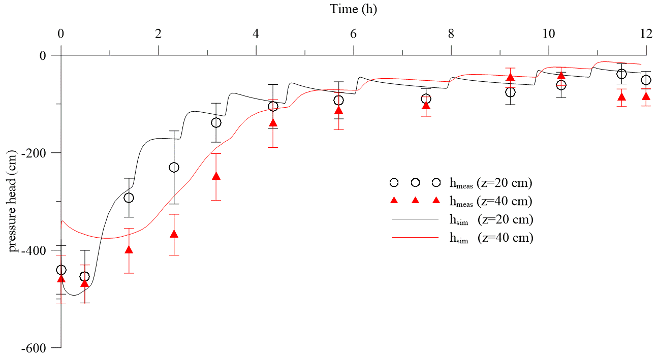
Figure 7 Evolution of pressure head at 20 and 40 cm depth measured by tensiometers (symbols) and estimated by the inversion procedure (lines) of the water infiltration process. The vertical bars represent the standard deviation of the measurements obtained by the four tensiometers.

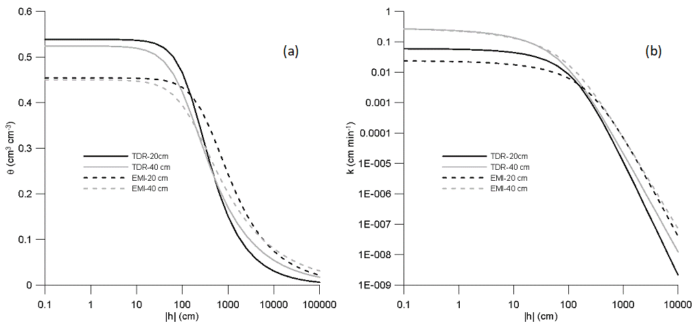
Figure 8 Soil water retention (a) and unsaturated hydraulic conductivity (b) curves, estimated from the TDR and EMI measurements at 20 and 40 cm depths.

Table 1 reports the parameters of the hydraulic functions, estimated for the first two horizons, and Fig. 8 reports the water retention curves and the hydraulic conductivity curves corresponding to the parameters shown in Table 1 for a better comparison between TDR-based and EMI-based hydraulic properties assessment. Compared to the Ap horizon, higher K_s and lower n values were found for the Bw horizon. This may be explained by considering that tillage in the Ap horizon changes the geometry of the porous system, by reducing the structural pores responsible for the lower K_s for Ap, and increasing the textural pores, explaining the higher n value for Ap. Note in the table the high values of n and K_s for the bedrock, which indicate a high conductive porous medium. It is possible to explain this by considering that the bedrock is fractured calcareous, which, contrary to expectations, does not impede water flow.

Table 1 van Genuchten–Mualem hydraulic parameters (Eqs. 7 and 8) and dispersivity, λ (Eq. 6) as estimated for Ap and Bw horizons, and fixed for the bedrock layer.

^* For all horizons θ_r=0 and τ=0.5.

As for water retention, the TDR and EMI water retention curves showed similar shapes but with slightly different saturated water content. As discussed earlier, the lower saturated water content is not surprising for the EMI-based estimation due to the overall underestimation of water content. The two curves almost overlapped after scaling the EMI curve by the ratio of the saturated water content. Obviously, this result is consistent with the underestimation of EMI-based θ distributions as shown in Fig. 6.

As for the hydraulic conductivity, TDR-based and EMI-based hydraulic conductivity curves at both 20 and 40 cm appear to almost overlap, with similar saturated hydraulic conductivity and curve shape. This result is expected because the shape of hydraulic conductivity curve is mainly explained by the variation of θ and not the absolute value of θ. It is worth mentioning that the same top boundary flux and different water content in the soil profile provided similar EMI-based and TDR-based hydraulic conductivity. These conditions led to two different water flow processes, with simulations predicting higher water stored in the soil profile and lower downward fluxes (data not shown) when TDR-based results are compared with the EMI-based results.

4.2 Solute infiltration – 2nd experiment

4.2.1 Time-lapse σ_a data and estimation ofσ_b distribution

Figure 9 shows the σ_a data collected during the solute infiltration experiment. Again, as for the 1st experiment, both VCP and HCP modes show a relatively similar pattern of σ_a values with ρ32 and ρ118 being the highest and lowest, respectively. The HCP mode shows higher values on average compared to the VCP mode. Similarly to the water infiltration experiment, σ_a increases consistently during the first 3 h of the experiment, then it does not change significantly or consistently until the end of the experiment. Much higher ranges of σ_a variations were measured in both VCP and HCP configurations, with σ_a values ranging at 20–200 and 50–250 mS m⁻¹ respectively.

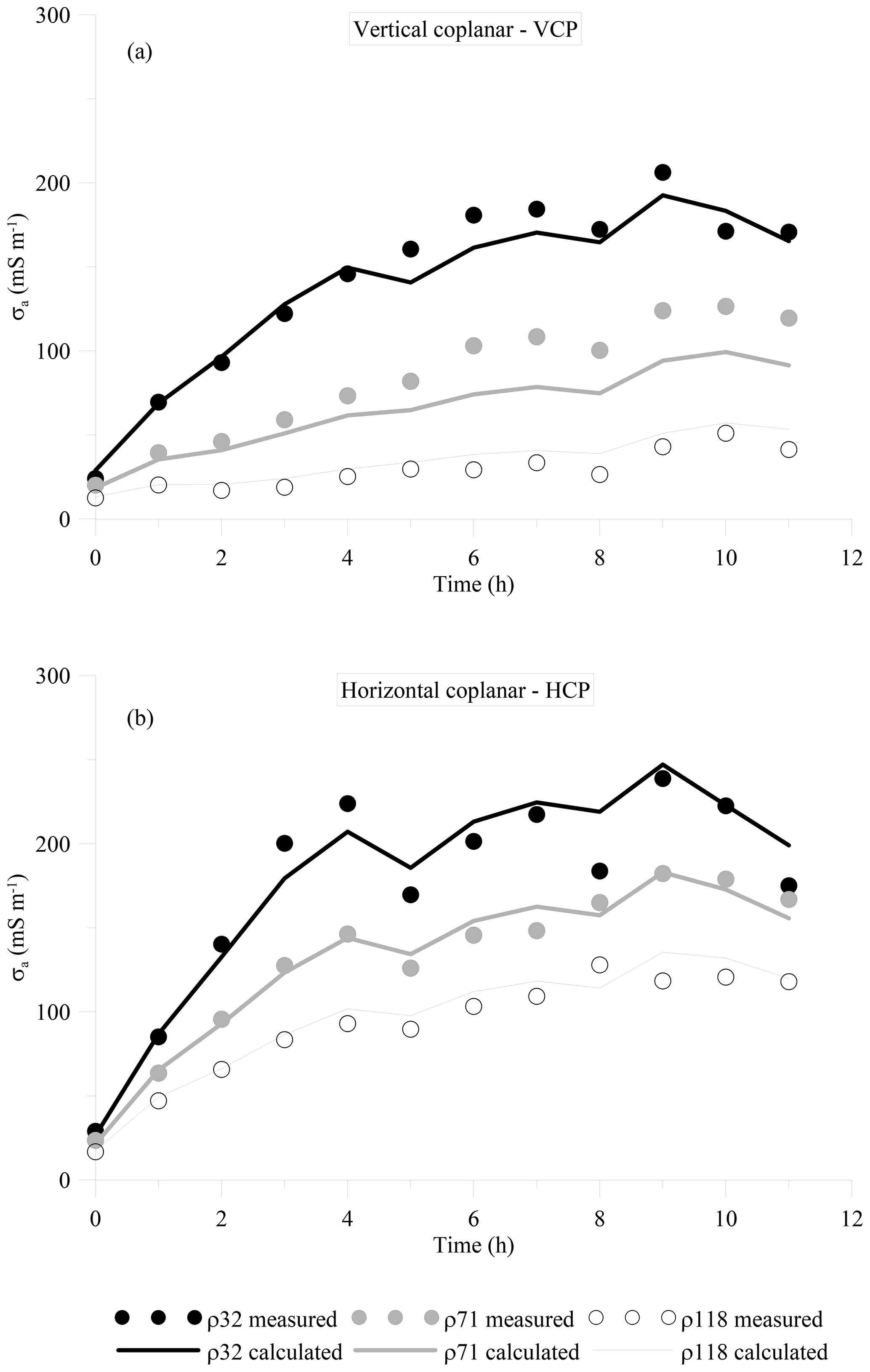
Figure 9 Values of σ_a observed during the solute infiltration experiment. (a) VCP, (b) HCP. The symbols represent the measured data whereas the lines represent the values calculated after the inversion.

Figure 10 depicts the σ_b evolution for the 2nd experiment, obtained by time-lapse inversion of σ_a data. The σ_a measurements and model response agree fairly well, as shown in Fig. 9; however, a slight shift can be noticed in the ρ71-VCP mode between the data and model response. The results show the rapid evolution of the conductive zone to the soil profile shortly after the irrigation started. In comparison with the obtained σ_b in the 1st experiment, the results reveal significantly higher soil conductivity in topsoil but a much slower evolution. The conductivity of the top layer exceeds 300 mS m⁻¹ shortly after the irrigation. The higher topsoil conductivity results from injection of high-saline water (about 15 dS m⁻¹) that dramatically increases soil conductivity, whereas the smaller evolution of the conductive zone is caused by a significantly slower concentration propagation into the soil profile.

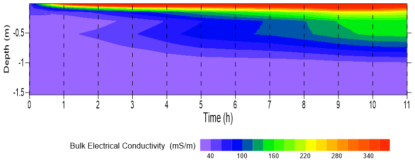
Figure 10 Time evolution of bulk electrical conductivity (σ_b) during the solute infiltration experiment.

4.2.2 Comparison between TDR-based and EMI-based σ_b and [Cl⁻] distributions

Figure 11 shows the comparison between the σ_b values obtained by the TDR measurements and those obtained from the EMI inversion (Fig. 10) during the 2nd experiment. As discussed earlier, this comparison is to provide insight into the potential of the EMI survey and inversion process in monitoring a solute transport experiment into a soil profile. The comparison shows a similar time pattern of σ_b variability, but in general the EMI model underestimates the σ_b obtained by TDR. The results of this comparison agree with the 1st experiment where, again, the EMI-based σ_b values are lower compared to those measured by the TDR. In contrast to the 1st experiment, the differences between the two techniques and in terms of the absolute σ_b values are of minor concern. This could be due to the larger conductivity contrast that tracer introduced into the soil profile in the 2nd experiment, which became easier to detect by using the EMI sensor. On the other hand, the TDR probes show more fluctuations in σ_b measurements, especially at 20 cm. We attribute these fluctuations to the smaller volume of investigation of the TDR probes, which are very sensitive to the process taking place very close to the probe and, therefore, strongly influenced by small-scale heterogeneities.

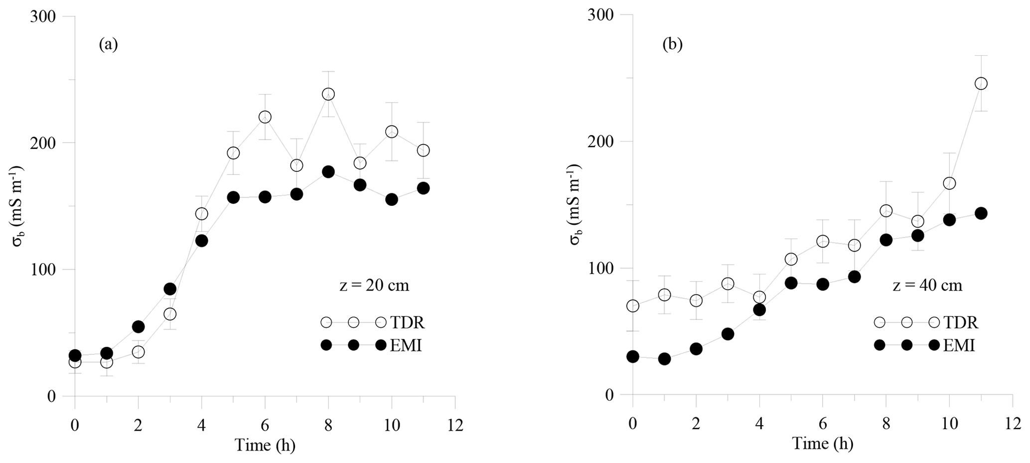
Figure 11 Evolution of σ_b as estimated by TDR and EMI measurements at 20 cm (a) and 40 cm (b) depth.

The next step in the procedure allows us to determine the distribution of Cl⁻ concentrations by EMI sensors (Sect. 4.2.3) used for estimating the longitudinal dispersivity of the two soil layers investigated. For the sake of comparison, TDR-based [Cl⁻] distributions were obtained directly in the field from a direct measurement of the σ_b. As for the EMI-based Cl⁻ concentrations, a forward HYDRUS-1D simulation was carried out using the EMI-based hydraulic properties obtained from the 1st experiment and reported in Table 1 to estimate the water content distributions corresponding to the EMI measurement times of the 2nd experiment. This water content, combined with the available σ_b distribution obtained from the EMI inversion, allowed us to obtain the σ_w distributions (through the θ–σ_b–σ_w calibration relationship) for both depths and, consequently, the [Cl⁻] distributions.

Figure 12 shows the [Cl⁻] distributions inferred from EMI compared to the TDR measurements. The comparison suggests a good agreement between the two time series. The EMI-based concentrations underestimate – on average – the TDR-based concentrations by 4 % and by 7 % at 20 and 40 cm depths, respectively. The time evolution of the two data series reveals marked differences, as shown by the very different correlation: $r=-\mathrm{0.04}$ for the 20 cm depth and r=0.70 for the 40 cm depth. The difference between the two data series at both depths can be mostly explained by the differences between σ_b distributions shown in Fig. 11. Additionally, another point of difference may arise from the assumption that the water content distribution obtained from the HYDRUS-1D simulation can be used as a substitute for the water content measurements, in order to obtain [Cl⁻] from the EMI readings.

Figure 12 [Cl⁻] distributions inferred from EMI and TDR measurements at 20 cm (a) and 40 cm (b) depth.

4.2.3 Estimation of longitudinal dispersivity

Inverse HYDRUS-1D simulations were conducted using concentration data provided by both the TDR and EMI results, in order to estimate the longitudinal dispersivity for both Ap and Bw horizons. The results are reported in the last row of Table 1. TDR-based and EMI-based procedures provide similar values of λ. Specifically, for the Ap horizon, the obtained values agree with those frequently found in the literature for either large columns or field-measured dispersivity (e.g., Vanderborght and Vereecken, 2007; Coppola et al., 2011). The TDR and EMI-based estimation of dispersivity for the Bw horizon shows 1 order of magnitude lower values compared to the Ap horizon. These values are more consistent with values measured in the laboratory (Coppola et al., 2019). For column scale (undisturbed soil monoliths with a length > 30 cm), Vanderborght and Vereecken (2007) found values in the order of 10 cm. The same values were found by Coppola et al. (2011) at both plot and transect scales. Note in Table 1 the high value of dispersivity used for the bedrock layer. This is consistent with the nature of the bedrock, which, as mentioned, is a fractured calcareous and highly conductive rock, which may well explain high dispersivity values.

5 Further discussion on three key points of the proposed approach

In the following, the discussion will focus on three major aspects of this research in terms of the choice of approach (uncoupled vs. coupled), the suitability of EMI as a replacement for invasive sensors, and EMI-related sources of uncertainty.

5.1 Uncoupled vs. coupled approach

In hydrogeophysical studies there is ongoing debate on this issue. Camporese et al. (2015) stated in their conclusions: “The relative merit of the coupled approach versus the uncoupled one cannot be assumed a priori and should be assessed case by case. As the information content of the geophysical data remains the same in both the coupled and uncoupled methods, the main difference is the approach taken in order to complement the information content and construct an “image of the process”. Based on the methodology proposed in this paper and the corresponding results, the following discussion aims to better clarify why we applied an uncoupled approach.

Let us refer to the vertical water infiltration process monitored by the EMI sensor during the 1st experiment and producing direct measurements of apparent electrical conductivity (σ_{a_meas}). In a coupled approach, the hydrological model is the starting point of the procedure. Guess values of hydraulic and dispersive parameters are initially fixed; thus, a hydrological simulation is carried out producing water content distributions along the soil profile, evolving over time. These water content distributions are converted to corresponding distributions of bulk electrical conductivity, σ_b, by using an empirical relationship (e.g., Binley et al., 2002). These σ_b distributions, in turn, are used as input in an EM forward modeling to produce the estimations of apparent electrical conductivity (σ_{a_est}). In this approach, the objective function involves the residuals (σ_{a_meas}−σ_{a_est}). This objective function is eventually minimized by optimizing the hydraulic parameters in the hydrological model.

The main strength of this approach relies on the fact that no EMI inversion is required. Also, as discussed by Hinnell et al. (2010), the attractiveness of the coupled approach is that the hydrological model may provide the physical context for a plausible interpretation of the geophysical measurements. Yet, this strength is counterbalanced by a weakness which is crucial in view of simplifying the experimental requirements of hydraulic characterization. In fact, an instrumental shift in EMI σ_a readings has been frequently observed when compared to other sources of measurements such as ERT data (von Hebel et al., 2014, 2019) or direct measurements of TDR (Dragonetti et al., 2018). In the context of a hydraulic parameter estimation procedure, this is a crucial point, as it means that EMI measurements do not immediately provide correct electrical conductivity distributions. Thus, the coupled approach always requires an independent dataset, obtained by different sensors (e.g., ERT, TDR, sampling) to remove the shift in the EMI σ_a readings. Such a scheme would be contrary to the essence of this paper, which mainly aims at minimizing the sensors and the data necessary for in situ soil hydraulic characterization.

In an uncoupled approach, the geophysical model is the starting point of the procedure. As a result of geophysical inversion, the σ_b distributions are derived, which are then converted to as many distributions of water content (θ_meas) through an empirical relationship, determined from laboratory analysis. Afterward, the hydrological model estimates water content (θ_est), and the objective function, involving the residuals (θ_meas−θ_est), is eventually minimized by optimizing the hydraulic parameters. The main weakness of this approach corresponds to the strength of the coupled approach. The uncoupled approach requires geophysical inversion, involving the uncertainty source coming from the ill-posedness problem. However, the main strength of the methodology we propose in this paper – a fast in situ noninvasive method to estimate soil hydraulic and transport properties at plot scale – does not require preliminary removal of the (unknown) shift in the EMI readings by additional field measurements with other sensors. Conversely, the shift effect is implicitly kept in the σ_b distributions, from these transferred to the measured EMI-based water content distributions and finally included in the hydrological inversion. This allowed us to reveal the effects of technical limitations of the EMI sensor, including the instrumental shift in EMI σ_a readings, on the water content estimations and thus on the estimation of the hydraulic properties. In the 1st experiment, by comparing the EMI-based water content with the water content coming from TDR, it was possible to see that the shift in the EMI readings produced quasi-parallel water content evolutions, thus meaning that the EMI shift is relatively stable with water content change. Related to this, in terms of hydraulic properties, the shift simply results in scaled saturated water content. This may well be explained physically by just considering that the parallel behavior of the water content over time signifies similar water content changes over time. This is translated into similar hydraulic conductivities, which in the vG–M model means similar α and n parameters, and thus water retention curves are simply scaled by the saturated water content ratio.

An additional benefit of an uncoupled approach is that it enables the sequential estimation of parameters (from the upper to the lower horizon), which can reduce the problems of parameter correlation and uniqueness. In this work, the parameters were estimated separately for each horizon of the profile according to Abbaspour et al. (1999). This approach makes parameter estimation of multi-layered profiles more feasible and accurate; however, this cannot be done within a coupled model. If more than one layer has to be characterized, the coupled approach requires that all the parameters be simultaneously optimized. This is because the electrical conductivity distribution of the whole soil profile must be first simulated in order to generate the required σ_{a_est} to compare to σ_{a_meas} in the objective function.

5.2 Suitability of EMI as a replacement for invasive sensors

The proposed methodology for the estimation of vG–M parameters proved to be effective for both Ap and Bw horizons. The overall EMI-based underestimation of θ did not impact the hydraulic conductivity curves significantly, as the shape of hydraulic conductivity is mainly explained by the θ variation and not by its absolute value. On the other hand, this underestimation resulted in lower saturated water content, which also appeared in the water retention curve. The latter can be simply converted to more accurate water content distribution by direct measurement of the actual saturated water content at the end of the experiment using TDR probes or even by taking soil samples for laboratory weight.

In terms of the longitudinal dispersivity, λ, there was a very good agreement between EMI-based and TDR-based estimation for both Ap and Bw horizons. The results are also in very good agreement with previous in situ and laboratory measurements. However, this method requires that the hydraulic properties of the investigated soil at the relevant scale be assessed prior to the application of this method to discriminate the contribution of water content and concentration in the EMI-based σ_b estimation.

5.3 EMI-related sources of uncertainty

The application of EMI for detailed investigation of the infiltration process has several limitations, apart from the potential instrumental drift of EMI sensor and the overall underestimation of water content and concentration, and requires further investigation. Resolving the wetting zone during the water injection is one source of uncertainty in this approach. The water content sharply decreases with depth in this zone close to the initial water content of the soil and causes dramatic resistivity variation. The limited number of σ_a measurements (total of 6) is not sufficient for recovering the sharp σ_b variability that takes place during the infiltration. In addition, a smoothness constraint was performed in the inversion process to stabilize the inversion process, which further smooths the layer boundaries in this approach. Resolving the shallow bedrock interface at depth and beneath a conductive zone was also very challenging. This is because the sensitivity of the EMI signals is generally very limited over the resistive zone and the condition becomes much worse when the resistive zone (bedrock) is located beneath a conductive zone (tracer): the EMI response of the subsurface is dominated by the influence of the near-surface conductive zone. In addition, five of the six depths of investigation of the CMD Mini-Explorer are limited to the first 1 m, and, as a result, a lower resolution is expected at greater depths. This resulted in an even larger underestimation of soil conductivity on top of the bedrock and an overestimation of bedrock conductivity in the close vicinity of soil. These findings from synthetic studies and modeling field data are similar to those reported in Farzamian et al. (2021) due to the similarity of the site and the experiment as well as the use of the same EMI sensor. Measuring σ_a at different heights or using different EMI sensors with a greater number of receivers such as the CMD Mini-Explorer 6L enables us to collect more σ_a data to better resolve changes that occur over short depth increments. To this end, the EMI configuration and data survey can also be optimized using optimization techniques such as machine-learning-based methods, given the specific survey goals and independent knowledge of the subsurface electrical properties, as shown, for example, by van't Veen et al. (2022).

6 Conclusion

In this paper, we proposed a noninvasive in situ method integrating EMI and hydrological modeling to estimate soil hydraulic and transport properties at the plot scale. For this purpose, we carried out two experiments involving (1) water infiltration and (2) solute transport over a 4×4 m plot. The propagation of wetting front and solute concentration along the soil profile in the plot was monitored using an EMI sensor (i.e., CMD Mini-Explorer) and, for the sake of procedure evaluation, TDR probes and tensiometers. Time-lapse apparent electrical conductivity (σ_a) data obtained from the EMI sensor were inverted to estimate the evolution over time of the vertical distribution of the bulk electrical conductivity (σ_b). The σ_b distributions were converted to water content and solute concentration by using a standard laboratory calibration, relating σ_b to water content (θ) and soil solution electrical conductivity (σ_w).

Based on the first water infiltration experiment, the soil water retention and hydraulic conductivity curves were then obtained for two layers of the soil profile by an optimization procedure minimizing the deviations between the numerical solution of the water infiltration experiment and the estimated water content inferred from the EMI results. EMI-based hydraulic properties were very similar in shape to those obtained by TDR and tensiometer data. This shape-similarity allowed us to convert the EMI-based hydraulic properties to the TDR-based ones by simply scaling them by the ratio of the saturated water content for both of the soil layers considered. This was a crucial finding in this paper and was mainly ascribed to the fact that the water content changes over time detected by the EMI closely followed those observed by TDR. These EMI-based hydraulic properties were then used as input for hydrological modeling of the second solute transport experiment. This made it possible to discriminate the water content and solute concentration components in the EMI σ_b distributions obtained during the second experiment. These concentrations were subsequently used to estimate the dispersivity based on an inversion procedure minimizing the residuals of EMI-based concentration and those simulated by the hydrological model. The reliability of the EMI-based hydraulic properties allowed us to obtain estimations of the dispersivity comparable to those obtained by the same optimization procedure applied to the TDR data.

The overall results show the great potential of the EMI sensor to replace TDR and tensiometer probes in the assessment of soil hydraulic properties. In practice, one could monitor a relatively short infiltration experiment with an EMI sensor and use the water content estimations in an inversion procedure to estimate the hydraulic properties. The underestimated water content observed in the first experiment can be converted to more accurate water content distribution by direct measurement of the actual saturated water content at the end of the experiment using TDR probes or even by taking samples and laboratory measurements.

The EMI-based estimation of longitudinal dispersivity, λ agrees well with TDR-based estimation as well as previous in situ and laboratory measurements, which suggests that the proposed methodology can be used in the assessment of this parameter that is indeed an important parameter in soil salinity simulations in salt-affected regions across the world. However, estimating λ based only on a solute infiltration test is not feasible as the temporal variability of σ_b is a function of both water content and concentration changes. We proposed the sequence of water and solute infiltration tests to discriminate the contribution of the water content and the soil solution electrical conductivity to the EMI-based σ_b.

Water irrigation and soil salinity management and thus hydrological investigations are usually field-scale and even large-scale challenges. The EM method is a noninvasive, fast, and cost-effective technique, covering large areas in less time and at a lower cost. Although this study was limited to a controlled experiment on a plot scale and a single study report, scaling up from plot-scale to field-scale assessment might be feasible due to the method's potential for rapid data collection. More investigations have to be conducted in this area to evaluate the potential of EMI sensors under different soil conditions and within the larger 2D and 3D investigations in order to further address the limitations of this methodology at different scales.