Effect of topographic slope on the export of nitrate in humid catchments: a 3D model study

Excess export of nitrate to streams affects ecosystem structure and functions and has been an environmental issue attracting worldwide attention. The dynamics of catchment-scale solute export from diffuse nitrogen sources can be explained by the changes of dominant flow paths, as solute attenuation (including the degradation of nitrate) is linked to the age composition of outflow. Previous data-driven studies suggested that catchment topographic slope has strong impacts on the age composition of streamflow and consequently on in-stream solute concentrations. However, the impacts have not been systematically assessed in terms of solute mass fluxes and solute concentration levels, particularly in humid catchments with strong seasonality in meteorological forcing. To fill this gap, we modeled the groundwater flow and nitrate transport for a small agricultural catchment in Central Germany. We used the fully coupled surface and subsurface numerical simulator HydroGeoSphere (HGS) to model groundwater and overland flow and nitrate transport. We computed the water ages using numerical tracer experiments. To represent various topographic slopes, we additionally simulated 10 synthetic catchments generated by modifying the topographic slope from the real-world scenario. Results suggest a negative correlation between the young streamflow fraction and the topographic slope. This correlation is more pronounced in flat landscapes with slopes $<\mathrm{1}:\mathrm{60}$. Flatter landscapes tend to retain more N mass in the soil (including mass degraded in soil) and export less N mass to the stream, due to reduced leaching and increased degradation. The mean in-stream nitrate concentration shows a decreasing trend in response to a decreasing topographic slope, suggesting that a large young streamflow fraction is not sufficient for high in-stream concentrations. Our results improve the understanding of nitrate export in response to topographic slope in a temperate humid climate, with important implications for the management of stream water quality.

1 Introduction

Globally nearly 40 % of land is used for agricultural activities (Foley et al., 2005), which constitutes the major source of pollution with nutrients such as nitrate (referred as to N–NO₃ in this study). Excess export of nitrate to streams threatens ecosystem structure and functions, and human health via drinking water (Vitousek et al., 2009; Alvarez-Cobelas et al., 2008; Dupas et al., 2017). This has been an environmental issue attracting attention in Germany and worldwide. The dynamics of nitrate export from diffuse nitrogen (N) sources are regulated by the dominant flow paths that determine the speed at which precipitation travels through catchments before it reaches the stream (Jasechko et al., 2016). The process is subject to both hydrological and biogeochemical influences mediated by various factors (e.g., catchment topography, aquifer properties, redox boundaries). From the perspective of sustainable intensification, process understanding and assessment of potential effects of catchment topography on nitrate export are critical for the management of water quality in connection with agricultural activity.

Field observations in central German catchments indicate that in-stream nitrate concentrations (C_Q) show significant differences in mean concentrations and seasonal variations between downstream areas with gentle topography and more mountainous upstream areas (Dupas et al., 2017; Nguyen et al., 2022). This provides strong evidence that catchment topographic slope can influence the nitrate export. In terms of water age analyses, Jasechko et al. (2016) using oxygen isotope data from 254 watersheds worldwide showed significant negative correlation between the young (age <3 months) streamflow fraction and the mean topographic gradient. They stated that young streamflow is more prevalent in flatter catchments as these catchments are characterized by shallow lateral flow, while it is less prevalent in steeper mountainous catchments as these catchments promote deep vertical infiltration. This statistically significant trend is consistent with the common finding that fast shallow flow paths produce young discharge and potentially influence the in-stream solute concentrations (Böhlke et al., 2007; Benettin et al., 2015; Hrachowitz et al., 2016; Blaen et al., 2017). However, apart from these data-driven analyses, a more mechanistic examination/explanation with the aid of fully resolved flow paths is still required. Wilusz et al. (2017) used a coupled rainfall–runoff and transit time model to investigate the young streamflow fraction, with a focus on the effect of rainfall variability rather than on topography and solute export. Zarlenga et al. (2022) numerically quantified the relative contributions of hillslopes and the drainage network to age dynamics in streamflow, considering the influences of transmissivity and recharge, without focusing on topographic slope. The effect of topographic slope on C_Q has rarely been subject to systematical testing.

Seasonal fluctuation of C_Q is commonplace in catchments under seasonal hydrodynamic forcing. Field observations in mountainous central German catchments indicate that nitrate concentrations, and the mass load, in streams vary seasonally, with maxima during the wet winter and minima during the dry summer (Dupas et al., 2017). Data-driven analyses by Musolff et al. (2015) and Dupas et al. (2017) suggested the systematic seasonal (de)activation of N source zones as an explanation for such seasonal variability. Under wetter winter conditions the near-surface N source zones in agricultural soils are connected to the stream by fast shallow flow paths. Under drier summer conditions, those N source zones are deactivated because their direct hydrologic connectivity to the stream is replaced with deeper flow paths (Dupas et al., 2017). Based on high-frequency monitoring in the Wood Brook catchment in the UK, Blaen et al. (2017) also reported mobilization of nitrate from the uppermost soil layers during high flow conditions via shallow preferential flow paths, which would not occur during base flow in drier periods. This behavior leads to a seasonally-variable nitrate loading due to changing flow paths and the associated variation in transit time that has been observed in many catchments (Benettin et al., 2015; Hrachowitz et al., 2016; Kaandorp et al., 2018; Rodriguez et al., 2018; Yang et al., 2018). However, how this fluctuation behaves in response to catchment land surface topography has not been assessed systematically yet. Such an assessment could improve our understanding of nitrate export from catchments of different topographic slopes not only in terms of the mean concentration but also regarding its temporal variation patterns.

Given that most of the above studies used data-driven analysis, numerical modeling is an effective tool for the analysis of water flow, age, and solute transport, eliminating the need for large amounts of field data. Zarlenga and Fiori (2020) presented a physically-based framework to model transient water ages at the hillslope scale, which was later used to investigate the different impacts of hillslopes and the channel network on water ages in catchments (Zarlenga et al., 2022). A number studies focused on numerically simulating the nitrogen fluxes (or loads) in soil and groundwater (Smith et al., 2004; Rivett et al., 2008; Lindström et al., 2010; van der Velde et al., 2012; Van Meter et al., 2017; Yang et al., 2018, 2019; Kolbe et al., 2019; Knoll et al., 2020; Nguyen et al., 2021, 2022). For example, van der Velde et al. (2012) constructed a lumped numerical nitrate transport model for the Hupsel Brook catchment in the Netherlands. Lindström et al. (2010) developed HYPE (Hydrological Predictions for the Environment) water quality model allowing for simulating the nitrogen fluxes in soil. Van Meter et al. (2017) investigated the two-centuries nitrogen dynamics in the Mississippi and Susquehanna River basins using a TTD-based (transient time distribution) transport approach. Yang et al. (2018) developed the coupled mHM–Nitrate model, which can provide valuable insights into the spatial variability of water and nitrate fluxes in catchment scale. Nguyen et al. (2021) further updated that model to the mHM–SAS model by implementing the SAS function-based solute transport module (Harman, 2015, 2019; Rinaldo et al., 2015; van der Velde et al., 2012), allowing for simulating the nitrate export from a mesoscale catchment. However, most of these works provided little information on the spatially explicit details (such as the flow field) for interpreting the nitrate dynamics. Physically-based hydrogeological models (e.g., HydroGeoSphere, Therrien et al., 2010) resolve the spatially explicit details within a catchment including the full variability of 3D flow paths in the subsurface, helping to understand the seasonally changing flow patterns in response to different catchment topographies. Additionally, the widely used fully-coupled surface–subsurface technology simulates the catchment as an integrated system, providing details of surface water–groundwater exchanges fluxes. These details help to identify paths of rapid discharge to the land surface that can considerably improve the interpretation of nitrate–export patterns.

Transit time distributions (TTDs) have been widely used to interpret hydrological and chemical responses in catchment outfluxes – both in discharge (Q) and in evapotranspiration (ET) (Botter et al., 2010, 2011; van der Velde et al., 2012; Heidbüchel et al., 2012; Rinaldo et al. 2015; Harman, 2015, 2019). They characterize how a catchment stores, mixes and releases water and dissolved solutes at large spatial and temporal scales (Benettin et al., 2015; Harman, 2015; van der Velde et al., 2010, 2012; Hrachowitz et al., 2015; Van Meter et al., 2017). Given that the nitrate attenuation is linked to the age composition of outflow, the TTDs are ideal tools for interpreting the concentration dynamics with regard to catchment topographic slope. Estimating water ages in natural catchments is still a challenge due to varying climate conditions, the errors in algorithms (e.g., errors in the flow field during particle tracking), and limited computational capacity. Yang et al. (2018) used particle tracking to compute the age distributions in the subsurface of a study catchment (while omitting the 4 % of total discharge produced by direct surface runoff and ignoring the frequent exchange fluxes that may be important for solute export due to their short transit times). Zarlenga et al. (2022) used a physically-based semi-analytical model to compute the transient water ages in a catchment, however, without considering surface runoff and hydrological losses (e.g., ET). In this study we determined the age compositions of Q and ET using numerical tracer experiments, where advective–dispersive transport of the tracers was solved using the fully-coupled surface–subsurface framework of HydroGeoSphere. The computed age dynamics based on the tracer concentrations were representative as the tracers were able to track all the flow processes such as surface runoff, groundwater flow, and surface–subsurface interaction.

In this study, we attempted to systematically assess the effect of catchment topographic slope on the nitrate export dynamics in terms of mass fluxes, concentration levels and its seasonal variability. We also seek mechanical explanations for the previously found behaviors from data-driven studies (e.g., Jasechko et al., 2016) with the help of fully resolved flow paths. First, we selected a real-world small agricultural catchment “Schäfertal” in Central Germany, which is characterized by strong seasonality in hydrodynamic forcing with associated shifts in the dominant flow paths (Yang et al., 2018). This catchment is typical for many catchments with hilly topography under a temperate humid climate. We created 11 model scenarios by adjusting the mean slope of the real-world catchment while preserving the aquifer heterogeneity. Next, we modeled the water flow and nitrate transport for each catchment. The flow and transport were solved using the fully coupled surface and subsurface numerical simulator HydroGeoSphere, and the water ages were computed using numerical tracer experiments. Finally, the modeled flow paths, water ages, N mass fluxes, and nitrate concentrations under various topographic slopes were analyzed. Through this study, we aimed to (1) examine the relationship between topographic slope and N mass fluxes, and to (2) assess C_Q and its seasonal variation in response to different topographic slopes.

2 Data collection

2.1 Real-world and synthetic catchments

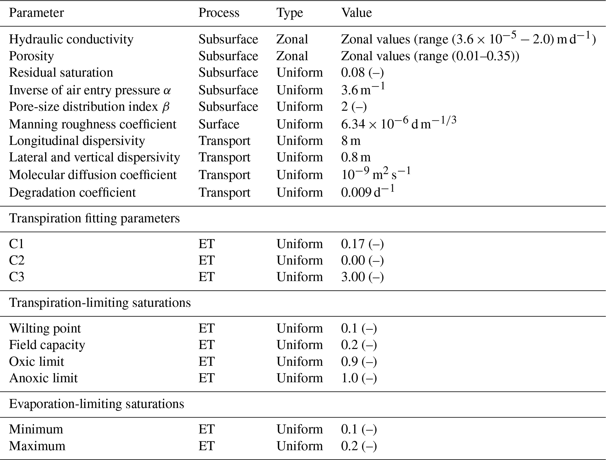
Our study was conducted on the catchment “Schäfertal”, situated in the lower part of the Harz Mountains, Central Germany (Fig. 1a). The catchment has an area of 1.44 km². The hillslopes are mostly used for intensive agriculture while the valley bottom contains riparian zones with pasture and a small stream draining the water out of the catchment. The gauging station at the outlet of the catchment provides Q records. This gauging station is the only outlet for discharging water from the catchment, because a subsurface wall was erected underneath the gauging station across the valley to block subsurface flow out of the catchment. A meteorological station 200 m from the catchment outlet provides records of precipitation (J), air and soil temperatures, radiation, and wind speed. The modeled catchment has a mean topographic slope of $\sim \mathrm{1}:\mathrm{20}$, estimated using a cross-section perpendicular to the stream (Fig. 1a). The aquifer thickness varies from ∼5 m near the valley bottom to ∼2 m at the top of the hillslope. Groundwater storage is low (∼500 mm) in such a thin aquifer and mostly limited to the vicinity of the channel with the upper part of the hillslopes generally unsaturated. The stream bed has a depth of 1.5 m below the land surface. Aquifer properties (e.g., hydraulic conductivity) change from the hillslope, dominated by Luvisols and Cambisols, to the valley bottom, dominated by Gleysols and Luvisols (Anis and Rode, 2015). Apart from that, the aquifer generally consists of two layers: the top layer of approximately 0.5 m thickness with higher porosity and a developed root zone from crops, and the base layer with smaller porosity due to high loam content (Yang et al., 2018). Subsequently, 10 property zones were used (Fig. 1b), with zonal parameter values following the model in Yang et al. (2018) listed in Table 1.

Based on this real-world catchment, 10 synthetic catchments were generated by adjusting elevations (land surface and aquifer bottom), such that the mean topographic slope ranges from 1:20 (steep) to 1:22, 1:25, 1:30, 1:40, 1:60, 1:80, 1:100, 1:200, 1:500, and 1:1000 (flat, Fig. 1b). The aquifer depth and heterogeneity were preserved during the adjustments. In total, 11 catchments were used for flow and transport simulations. The catchment with the original topography (1:20) is selected as the base scenario.

2.2 Climate

The considered climate for the catchments was derived from the catchment “Schäfertal” located in a region with temperate humid climate and pronounced seasonality. According to the meteorological data records from 1997 to 2007, the mean annual J and Q (per unit area) are 610 and 160 mm, respectively. Actual mean annual ET based on the 10 yr water balance ($J=\text{ET}+Q$) is 450 mm. Mean annual potential ET is 630 mm (Yang et al., 2018). The humid climate is representative for wet regions, quantified by an aridity index (J/potential ET (Li et al., 2019) of 1.0. The ET is the main driver of the hydrologic seasonality as the precipitation is more uniformly distributed across the year (Fig. 1c).

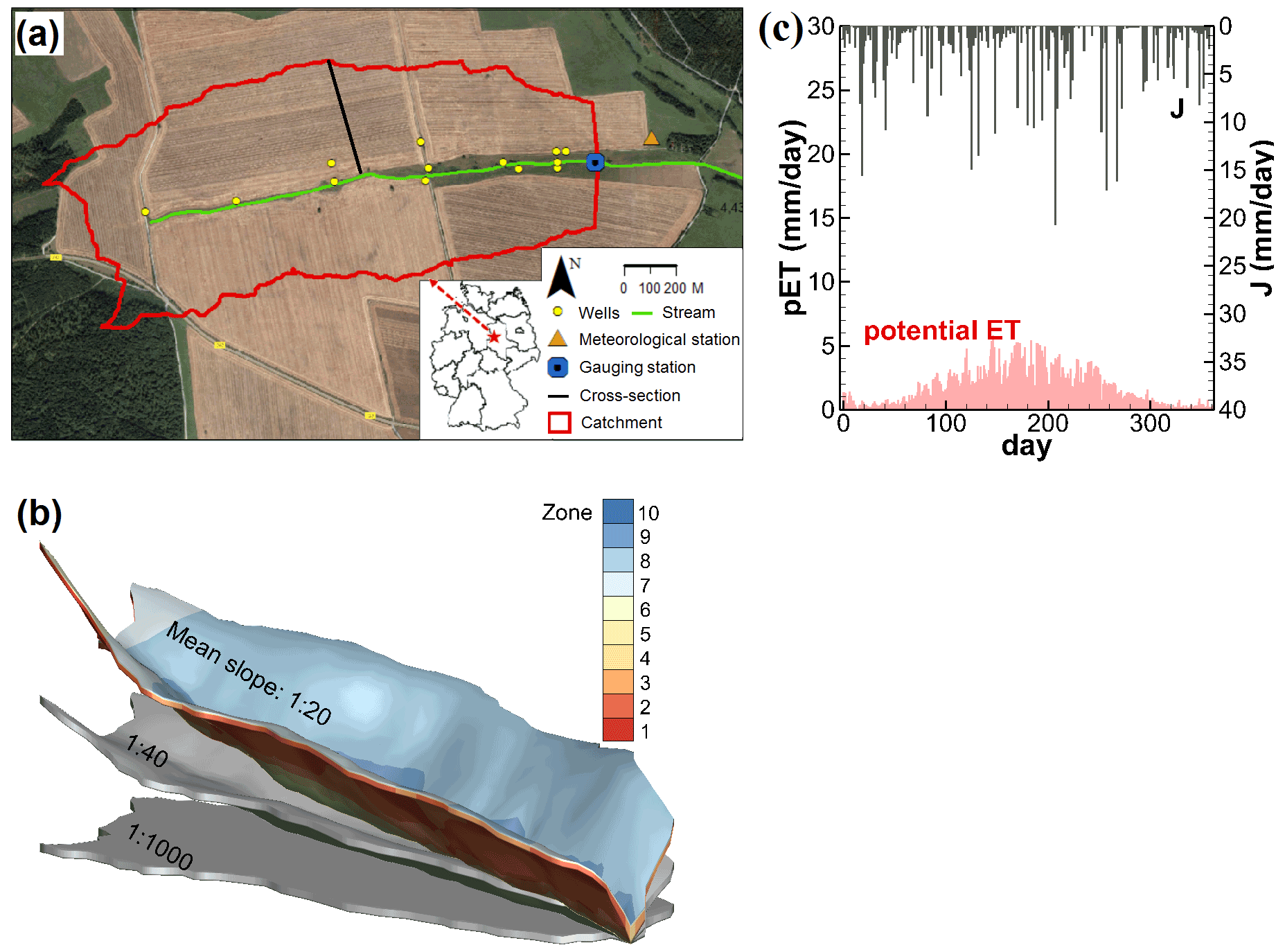
Figure 1 (a) The catchment “Schäfertal”, Central Germany (background image from © Google Maps). (b) The catchments with mean topographic slopes of 1:20, 1:40, and 1:1000. (c) The measured precipitation J and the estimated potential evapotranspiration ET for the year 2005 under the humid climate (Yang et al., 2018). Ten aquifer property zones in (b) were defined in the subsurface of the catchment for zonal parameter values (e.g., hydraulic conductivity).

3 Methods

3.1 Flow and nitrate transport

3.1.1 Flow model

It is necessary to solve both groundwater and surface water flow because the spatially-explicit details in the catchment including the specific flow paths and exchange fluxes are necessary to interpret the effect of varying topographic slope on nitrate transport. We simulated the flow system using the fully coupled surface and subsurface numerical model HydroGeoSphere, which solves for variably saturated groundwater flow with the Richards' equation and for surface flow with the diffusion-wave approximation of the Saint-Venant equations (Therrien et al., 2010). Additionally, the exchange flux between groundwater and surface water can be implicitly simulated. The nitrate transport is simulated in the groundwater flow, surface flow, and exchanges fluxes by solving the advection–dispersion–diffusion equation describing the conservation of nitrate mass. HydroGeoSphere has been successfully used to simulate catchment with hydrological processes and solute transport in many studies (e.g., Therrien et al., 2010; Yang et al., 2018), therefore governing equations and technical details are not explicitly repeated here.

In our previous work of Yang et al. (2018), a hydrological flow model has already been established for the catchment “Schäfertal”. It was calibrated against measured groundwater levels and stream discharge Q. The optimized parameter values are listed in Table 1. In this work, we performed our simulations based on that flow model, with the nitrate transport process being added while maintaining the model setup. We provide a brief review of that flow model here. Readers may refer to Yang et al. (2018) for a full description of the model and its calibration.

The modeled subsurface of the catchments was discretized into nine horizontal layers between the land surface and the aquifer base, with thinner layers in the upper part (0.1 m) to better represent the unsaturated zone and compute the ET. In total, the subsurface was discretized by a mesh of 13 860 prisms, with the horizontal size of the prisms ranging from 30 to 50 m. The topmost 1540 triangles were used to discretize the surface domain, where surface flow was simulated. Ten property zones for the subsurface were defined (Fig. 1b), being assigned with the zonal hydraulic conductivity and porosity values (Table 1). ET was simulated as a combination of plant transpiration from the root zone (top 0.5 m soil) and evaporation down to the evaporation depth (0.5 m), which are both constrained by soil water saturation. Regarding the flow boundary conditions, spatially uniform and temporally variable J was applied to the land surface. Spatially constant and temporally variable potential ET was applied to the aquifer top to calculate the actual ET. The bottom of the aquifer was considered an impermeable boundary. A critical depth boundary condition was assigned to the catchment outlet to simulate the stream discharge Q, which was compared to the measured Q during the calibration. The software PEST (Doherty and Hunt, 2010) was used for the transient calibration. After calibration, the time-variable groundwater levels were well-replicated by the flow model for most of the wells, with mean coefficients of determination (R²) of 0.43. The fit between the simulated and measured Q was satisfactory with a R² of 0.61. The calibrated model successfully simulated the flow system from 1997 to 2007.

In this study, we continued to use the above-described model setup, including the mesh, the parameters, and the flow boundary conditions, for the 11 catchments with different topography. Note that the mesh was adapted to the change of the topography by changing node elevations vertically. However, to simplify the flow simulation and the age computation (described in Sect. 3.2), we selected the year 2005 as a representative year and assumed that all the years have the identical climate (J and potential ET) as the year 2005. Therefore, J and potential ET of 2005 (Fig. 1c) were cycled and applied to the catchments for all the simulated years.

Table 1 The key flow parameters and their values following Yang et al. (2018).

3.1.2 Transport boundary conditions and parameters

The nitrogen (N) pool is formed in the soil zone of the catchments, representing a nitrate source zone. The N pool is controlled by various complex processes. It is replenished by external inputs from atmospheric deposition, biological fixation, animal manure from the pasture area, and fertilizer from the farmland on the hillslopes. Nitrate that can be transported with water is formed and leached from this N pool by a microbiological immobile–mobile exchange process (Musolff et al., 2017; Van Meter et al., 2017). In our study, we employed the simplified framework by Yang et al. (2021) to track the fate of N in the N pool (Fig. 2a). This framework was derived from the ELEMeNT approach (Exploration of Long-tErM Nutrient Trajectories, Van Meter et al., 2017), which uses a parsimonious modeling framework to estimate the biogeochemical legacy nitrate loading in the N pool and the N fluxes leaching from the N pool to the groundwater. This framework assumes that total N load in the N pool is comprised by inorganic N (SIN) and organic N (SON). Two types of SON are distinguished: active organic N (SON_a) with faster reaction kinetics and protected organic N (SON_p) with slower reaction kinetics. It is assumed that the external N input contributes only to the SON. The SON is mineralized into SIN. The SIN is further consumed by plant uptake and denitrification, and finally leaches to groundwater as dissolved inorganic N (DIN), representing mainly nitrate in the studied catchment (Yang et al., 2018; Nguyen et al., 2021). The framework is acceptable due to the fact that most of the nitrate fluxes from source zones has undergone biogeochemical transformation in the organic N pool (Haag and Kaupenjohann, 2001). The framework simplifies complexities of different N pools and transformations via mineralization, dissolution, and denitrification within the soil zone (Lindström et al., 2010), while preserving the main pathway for nitrate leachate.

The governing equations to calculate these N fluxes follow the ones in Yang et al. (2021). A specific portion (h) of the external N input contributes to the SON_p pool, and the rest contributes to the SON_a pool. The portion h is the land use-dependent protection coefficient (Van Meter et al., 2017). The mineralization and denitrification are described as first-order processes with rate coefficients k_a, k_p, and λ_s respectively, using

$$\begin{array}{}\text{(1)}& {\displaystyle }{\text{MINE}}_{\text{a}}=k_{\text{a}}\cdot f\left(\text{temp}\right)\cdot {\text{SON}}_{\text{a}}\text{(2)}& {\displaystyle }{\text{MINE}}_{\text{p}}=k_{\text{p}}\cdot f\left(\text{temp}\right)\cdot {\text{SON}}_{\text{p}}\text{(3)}& {\displaystyle }{\text{DENI}}_{\text{s}}={\mathit{\lambda }}_{\text{s}}\cdot \text{SIN},\end{array}$$

where MINE_a, MINE_p, and DENI_s (kg ha⁻¹ d⁻¹) are the mineralization rates for SON_a and SON_p, and denitrification rate for SIN. k_a, k_p, and λ_s (d⁻¹) are coefficients for the first-order processes. f(temp) is a factor representing a constraint by soil temperature (Lindström et al., 2010). Note that the mineralization and plant uptake occur in the N pool. Denitrification can occur in both the N pool and later in groundwater. The plant uptake rate UPT follows the equation used in the HYPE model (Lindström et al., 2010),

$$\begin{array}{}\text{(4)}& {\displaystyle }\text{UPT}=\text{min}\left({\text{UPT}}_{\text{P}},\mathrm{0.8}\cdot \text{SIN}\right)\text{(5)}& {\displaystyle }\begin{array}{rl}& {\text{UPT}}_{\text{P}}=p\mathrm{1}/p\mathrm{3}\cdot \left({\displaystyle \frac{p\mathrm{1}-p\mathrm{2}}{p\mathrm{2}}}\right)\cdot e^{-(\text{DNO}-p\mathrm{4})/p\mathrm{3}}/\\ & {\left(\mathrm{1}+\left({\displaystyle \frac{p\mathrm{1}-p\mathrm{2}}{p\mathrm{2}}}\right)\cdot e^{-\left(\text{DNO}-p\mathrm{4}\right)/p\mathrm{3}}\right)}^{\mathrm{2}}\end{array},\end{array}$$

where UPT and UPT_P (kg d⁻¹ ha⁻¹) are the actual and potential uptake rates. The computation of UPT_P considers a logistic plant growth function. DNO is the day number. $p\mathrm{1},p\mathrm{2},andp\mathrm{3}$ are three parameters depending on the crop/plant type, they are in the units of (kg ha⁻¹), (kg ha⁻¹), and (day), respectively. p4 is the day number of the sowing date. The leaching process allows for SIN to leach from the soil (N pool) to the groundwater. The leaching rate LEA (kg ha⁻¹ d⁻¹) is defined as a first-order process as

$$\begin{array}{}\text{(6)}& {\displaystyle }\text{LEA}=f\cdot \text{SIN}/\mathrm{\Delta }t\text{(7)}& {\displaystyle }f=(\mathrm{1}-{\exp }^{-a\frac{\text{wal}}{\mathit{\theta }d}})\text{(8)}& {\displaystyle }\text{wal}=q\cdot \mathrm{\Delta }t,\end{array}$$

where f is a factor, ranging between (0, 1), to determine the portion of SIN that leaches into groundwater during a time step Δt. a is unit-less leaching factor. θ is the soil porosity. d is the soil depth. wal (L) is the water available for leaching during Δt. wal can be estimated using the Darcy fluxes q (LT⁻¹), which are provided by the flow simulations for each cell of the mesh. Physically, f is a function of the ratio between wal and the volume of soil voids θ⋅d, representing the ability of water to flush the SIN. This formulation of LEA is modified from the ones used in Pierce et al. (1991), Shaffer et al. (1991), and Wijayantiati et al. (2017) to comply with the spatially distributed HydroGeoSphere model.

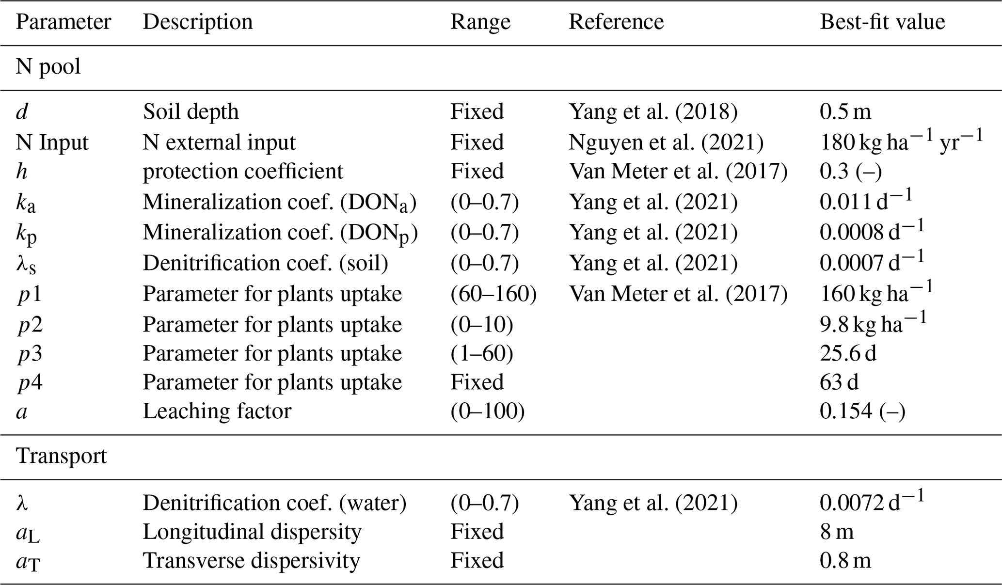
Table 2 The parameters for the N pool and nitrate transport. The parameters with a range are calibrated. The adjustable ranges are selected to cover the values that the parameters can potentially take on or the values reported by the referred literature.

The N pool is positioned on the top part of the aquifer, used as a boundary condition for the DIN (nitrate) transport. Advective–dispersive transport of DIN in the flow system is simulated using HydroGeoSphere (Fig. 2b). Degradation (denitrification in groundwater) during transport is considered as a first-order process. Degradation is not considered on the land surface (denitrification in surface flow), where aerobic conditions likely deactivate denitrification and residence time is short. To implement the evapoconcentration effect in the transport model, ET is assumed to remove DIN mass without altering the DIN concentration of the water, and to inject that mass back to the SIN pool. This represents a precipitation process from DIN to SIN, which is the inverse process of leaching (Fig. 2b). There are two reasons for doing that: (i) the physical process of ET causing the immobilization of DIN can be mathematically considered, and (ii) the N mass balance can be conserved as the plants uptake is already considered in the N pool according to the plant growth function (Eqs. 4 and 5), being independent from the ET flux.

Regarding the parameters, the soil depth, within which the N pool is implemented, is set to 0.5 m. N external input is 180 kg ha⁻¹ yr⁻¹ according to Nguyen et al. (2021), where the nitrate balance was simulated for the larger upper Selke Catchment that contained our studied catchment. The external N input is assumed to be spatiotemporally constant due to the limited information on its variation in space and time. The protection coefficient h is fixed as 0.3 according to the values reported in Van Meter et al. (2017). The sowing date p4 is fixed as 63 d according to the fact that sowing activities and plant growth start in early March. Longitudinal and transverse dispersivity values were 8 and 0.8 m, respectively. Other parameters were set to be adjustable and calibrated (Table 2).

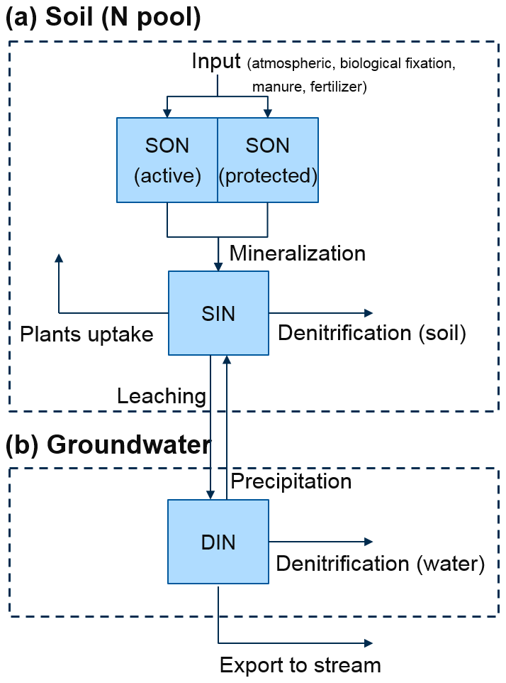
Figure 2 Conceptual framework for nitrogen (N) fluxes (a) in the soil (N pool), and (b) after leaching into the groundwater.

3.1.3 Transport calibration

As the flow parameters (e.g., hydraulic conductivity and porosity) were already calibrated in Yang et al. (2018) using data sets of discharge and groundwater levels, in this study the calibration was only performed for the transport to get reasonable parameter values for the N pool and N transport. The software package PEST (Doherty and Hunt, 2010) was used. PEST uses the Marquardt method (Marquardt, 1963) to minimize a target function by varying the values of a given set of parameters until the optimization criterion is reached. We used the measured C_Q and N surplus as the target variables for comparison with the simulated ones. The N surplus, which is the annual amount of N remaining in the soil after consumption by plant uptake, was estimated as 48.8 kg ha⁻¹ yr⁻¹ (Yang et al., 2021). As two different data sets (C_Q and N surplus) were used, a weighting scheme was used such that the defined multi-objective function was not dominated by one data set.

Note that the entire model calibration (for flow and transport) actually followed a procedure of two steps: first for flow, and second for transport. Alternatively, the flow and transport parameters can be calibrated at one step by defining the multi-objective function using all the data sets (discharge, groundwater levels, C_Q, and N surplus). The potential effect of the two different calibration procedures on the modeling results should be further explored, however it is out of the main focus of this study. We consider the two-step calibration procedure to be acceptable, because our result showed that it was sufficient to reach an acceptable model performance for both flow and transport (described later).

Several transport parameters were fixed at the values selected according to prior information, such that the degree of freedom in the calibration can be reduced as much as possible (Table 2). In total, eight parameters were adjustable and calibrated, because they were the key parameters to determine the N fluxes in soil and groundwater. Their adjustable ranges were selected according to the literature or to cover the values that the parameters can realistically reach (Table 2). The calibration was carried out for the period from July 1999 to July 2003, during which the data sets are available. First, the flow and transport were simulated in the catchment of the base scenario (original topography, Sect. 2.1). Secondly, PEST was used to obtain a best fit between the simulated results and the data sets by varying the parameter values. Note that the simulation period from July 1999 to July 2003 was only used for model calibration, rather than for the actual simulations with the 11 catchments of different topographic slope. After calibration, the model with the best-fit parameter values can well-replicate the measured C_Q with a Nash–Sutcliffe efficiency (NSE) of 0.75 (see Fig. S1 in the Supplement). The simulated N surplus was 50.7 kg ha⁻¹ yr⁻¹, comparable to the measured value.

The best-fit parameter values from the base scenario were used for all other scenarios with catchments of different topographic slope, assuming that the parameters do not change with the change of topographic slope. In total, we simulated the flow and nitrate transport for 11 scenarios (11 catchments of different topographic slope). For each scenario, the simulations were run for 100 yr with identical boundary conditions for each year. The first 99 yr were used as a spin-up phase to assure a dynamic equilibrium (i.e., to achieve simulated variables, such as heads and concentrations, that are identical between years), and the last year was used for actual observation and analysis. The CPU time of each simulation was ∼4 h.

3.2 Water ages

The water stored in a catchment (storage), Q, and ET can all be characterized by age distributions, for they comprise water parcels of different age from precipitation events that occurred in the past. The age distributions need to be calculated for each aforementioned scenario to assess the responses of water ages on catchment topographic slope. Our model setup (with virtual catchments and identical climate for each year) allowed us to perform long-term numerical tracer experiments and to extract the age distributions.

We assumed that inert tracers of uniform concentration existed in precipitation. The tracers were applied to the land surface as a third-type (Cauchy) boundary condition and were subjected to transport modeling. Tracer can exit the aquifer via the outfluxes Q and ET. We considered a period of 200 yr for the tracer experiments, which was sufficiently long to ensure convergence of the computed water ages. The 200 yr period was partitioned into 2400 months (Δt=1 month). A different tracer was used for each of the periods resulting in a total of 2400 distinct tracers. The injection of tracer i started with the precipitation at the beginning of its associated period $t_{\mathrm{0}}^i$ and lasted throughout the period. The advective–dispersive multi-solute transport was simulated using HydroGeoSphere. The first 199 yr of the simulation period were used as a spin-up phase to ensure a dynamic equilibrium of the calculated ages, minimizing the influence of the initial conditions. The last year was used for the actual observations and the computation of age distributions. Solving the transport of the 2400 tracers would be computationally expensive. However, because the climate (flow boundary conditions) was identical for each year, the transport simulation was performed only for the first 12 tracers that covered the course of a year. Based on these results, the results for the other 2388 tracers were manually reproduced (e.g., by shifting the concentration breakthrough curves of the 12 tracers in time while maintaining the shapes).

For each tracer, the breakthrough curves of the mass fluxes of Q and ET, and the mass in storage were reported. For a specific time t, the age distributions for Q/ET/storage were computed by calculating the mass fraction of each tracer using

$$\begin{array}{}\text{(9)}& p_{Q/\text{ET}/S}(T,t)={\displaystyle \frac{M^i\left(t\right)}{\mathrm{\Delta }t\sum M^i\left(t\right)}},\end{array}$$

where p_Q(T,t) and p_ET(T,t) are the age distributions of Q and ET (equivalent to backward transit time distributions – TTDs), and p_s(T,t) is the age distributions of water in storage (equivalent to the residence time distribution – RTD). Mⁱ(t) is the mass flux of the tracer i in Q or ET, or the mass stored in catchment at time t, and ∑Mⁱ(t) is the sum of Mⁱ(t) over all tracers. T is the age ranging within $(t-t_{\mathrm{0}}^i-\mathrm{\Delta }t,t-t_{\mathrm{0}}^i$) for tracer i.

For each scenario, the CPU time of the tracer experiment was ∼8 h. Based on the age distributions, we calculated the mean discharge age T_Q(t), which is equivalent to the mean discharge transit time (simply referred to as “discharge age” in the following sections). We calculated the young water fraction in streamflow YF_Q(t), which is the fraction of streamflow with an age younger than 3 months (also referred to as “young streamflow fraction” (Jasechko et al., 2016). Similarly, the ET age T_ET(t) and the young water fraction in ET YF_ET(t) can be calculated as well (more details are described in Sect. S1 in the Supplement). Their responses to changes in topographic slope were analyzed.

4 Results and discussion

4.1 Dynamics of water ages and nitrogen fluxes

Driven by the seasonality of the climate, the simulated Q, the young water fractions YF, and the water ages all show seasonal fluctuations. Figure 3 shows these fluctuations for the base scenario (original topography). Q reaches its maximum towards the end of the wet winter in late February and reaches its minimum during the drier late summer in mid-September. Total Q consists of a portion of groundwater discharge (including the flow via vadose zone) and a portion generated via surface runoff during events of high precipitation (Fig. 3a). The calculated YF_ET is smallest in April and largest in November (Fig. 3b), while YF_Q is smallest in August and largest in February. ET generally has larger young water fractions than Q as ET has a higher probability to remove young water from the shallow soil rather than the older water from the deeper aquifer. Especially during the dry season (summer), most precipitation can be quickly removed by ET. The water ages of Q and ET show generally opposite fluctuation patterns for YF (Fig. 3c). The ET age ranges from 70 to 115 d, being younger than Q that has the age ranging from 109 to 180 d.

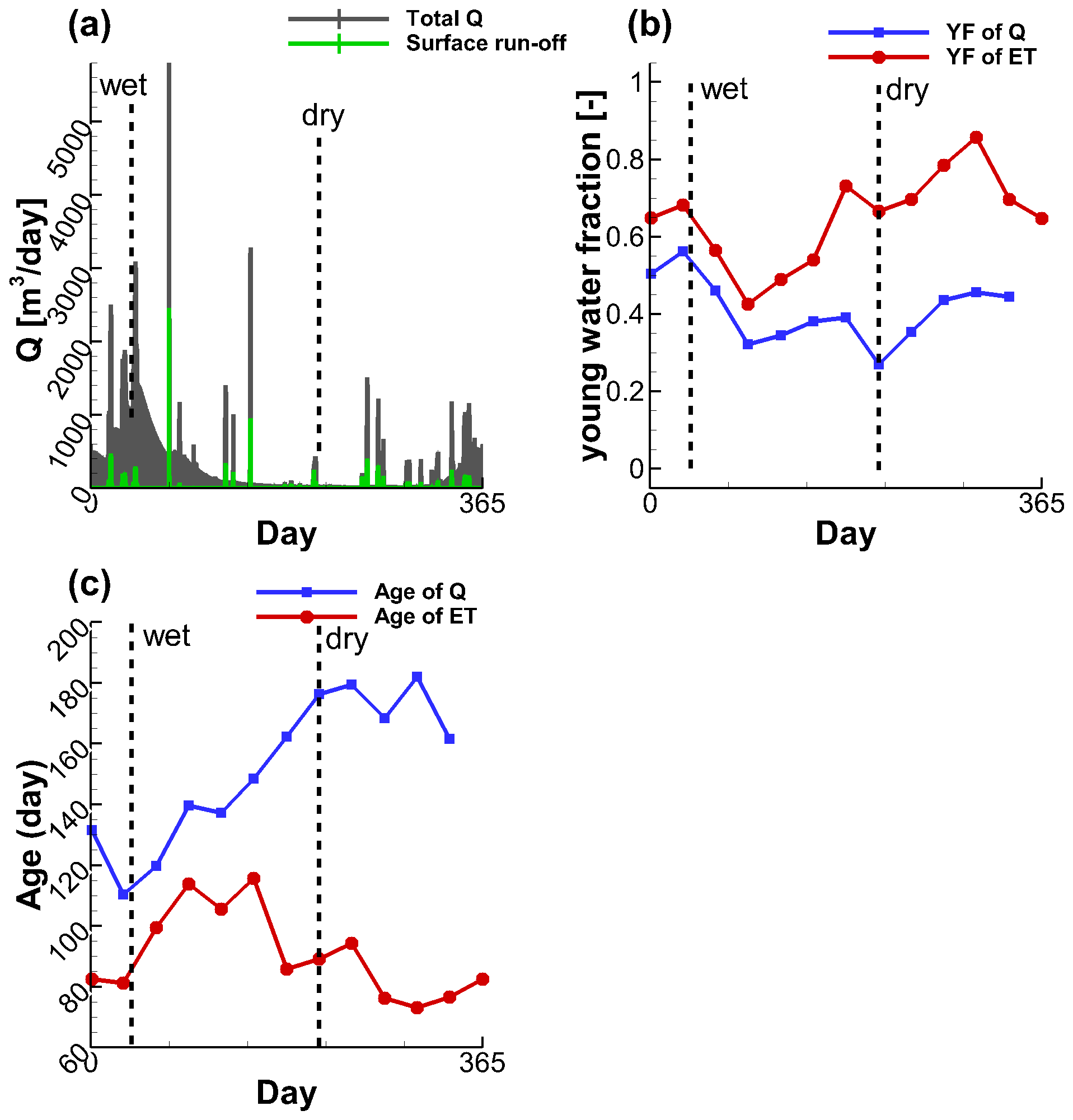
Figure 3 Simulated (a) Q, (b) young water fractions in streamflow (YF_Q) and evapotranspiration (YF_ET), and (c) water ages for the catchment of the base scenario. The YF and water ages are monthly averages.

The simulated C_Q shows strong seasonality with maxima in the wet and minima in the dry period, fitting the measured C_Q data well (Fig. 4a). Figure 4b lists the calculated annual N mass balance in the catchment of the base scenario. The organic (SONa + SONp) and inorganic (SIN) N load in the soil are 470 and 43 kg ha⁻¹, respectively. The SON accounts for 92 % of the total N load, which is consistent with the study of Stevenson (1995) where the organic N fraction was reported to be greater than 90 %. The mineralization converts SON into SIN with a rate of 180 kg ha⁻¹ yr⁻¹. This rate is equal to the external N input because this way a steady state of the annual N mass balance was reached in the simulations. About 76 % of the input N flux is taken up by the vegetation (136 kg ha⁻¹ yr⁻¹) and 20 % is consumed by denitrification (36 kg ha⁻¹ yr⁻¹), either in the soil (before leaching) or in the groundwater (after leaching). The remaining 4 % reaches the stream water and is exported out of the catchment (6 kg ha⁻¹ yr⁻¹). The simulated mineralization flux is within the range of (14–187) kg ha⁻¹ yr⁻¹ reported by Heumann et al. (2011) for their study sites in Central Germany. The simulated plant uptake and leaching fluxes are comparable to the values suggested in Nguyen et al. (2021) for the same area (120 kg ha⁻¹ yr⁻¹ for plant uptake and (15–60) kg ha⁻¹ yr⁻¹ for leaching). The simulated denitrification rate is within the range (8–51) kg ha⁻¹ yr⁻¹ reported in Hofstra and Bouwman (2005) for 336 agricultural soils located worldwide. Moreover, 80 % and 20 % of the leaching N are consumed by denitrification during transport in the groundwater and exported to stream water, respectively. These portions are generally comparable to those reported in Nguyen et al. (2021) (61 % and 39 %, respectively). Therefore, the simulated N loads and fluxes for the catchment of the base scenario are considered to be acceptable.

Figure 4c shows the temporal variation of the N load and fluxes. It demonstrates that low levels of SIN are maintained by high plant uptake before the dry summer arrives (May–June), such that there is little SIN available for leaching. The SIN load reaches its minimum when plant uptake reaches its maximum (marker a in Fig. 4c). The cessation of plant uptake during the dry period leads to the increase of the SIN load and the increase of the leaching rate. The mineralization in winter is significantly reduced due to the dropping temperatures, cutting the SIN supply. This results in the SIN load reaching its high peak in the middle of November (marker b in Fig. 4c) and subsequent decrease due to increased leaching and eventually plant uptake. These seasonal fluctuation patterns are generally consistent with the knowledge of N fluxes reported in previous studies (Dupas et al., 2017; Nguyen et al., 2021). For DIN load in water, it reaches its maximum generally when the leaching weakens in the beginning of March (marker c in Fig. 4c), and reaches the minimum just before the leaching process becomes active again in the end of August (marker d in Fig. 4c). These low and high peaks of SIN and DIN loads can also be identified by their spatial distributions in the catchment (see Fig. S2).

Seasonal variations of C_Q can be directly influenced either by the fluctuation of the nitrate leaching into groundwater, or by fluctuations in the degradation in groundwater associated with varying transit times (quantified by the young water fraction in streamflow YF_Q). These two influences represent the effect from the variability in N source and in N transport, respectively. Linear regression analysis shows that C_Q is correlated with leaching flux rate and YF_Q with Spearman rank correlation coefficients of 0.1 and 0.34, respectively (Fig. 5). The seasonal fluctuations of C_Q and leaching flux are temporally out of phase. The maximum leaching occurs in December, while the maximum C_Q is reached 2 months later in February (Fig. 5a). The minimum leaching occurs in April, while the minimum C_Q is reached around September. This behavior indicates that C_Q responds later to the changes in N leaching, which is reasonable because the leaching nitrate needs time to travel from the shallow soil to streamflow. The fluctuation of C_Q and YF_Q are more synchronized, proven by the fact that both maxima are reached in February (wet, Fig. 5b) and minima occur generally in the dry summer time. Field observations in mountainous central German catchments also indicate that C_Q varies seasonally, with maxima during the wet winter and minima during the dry summer (Dupas et al., 2017). These seasonal fluctuations of C_Q and YF_Q were frequently explained using the “inverse storage effect” (Harman, 2015; Yang et al., 2018) as during the wet season Q has a strong preference for young water associated with higher concentrations, which would not occur during dry periods due to the deactivation of the shallow fast flow processes. These patterns generally suggest that the C_Q fluctuation is more attributed to the variability in the N transport rather than to the variability in the N source, echoing previous observations that 80 % of the leaching N mass is degraded during transport. However, it is still hard to tell whether the N source or the N transport is dominating the C_Q fluctuation.

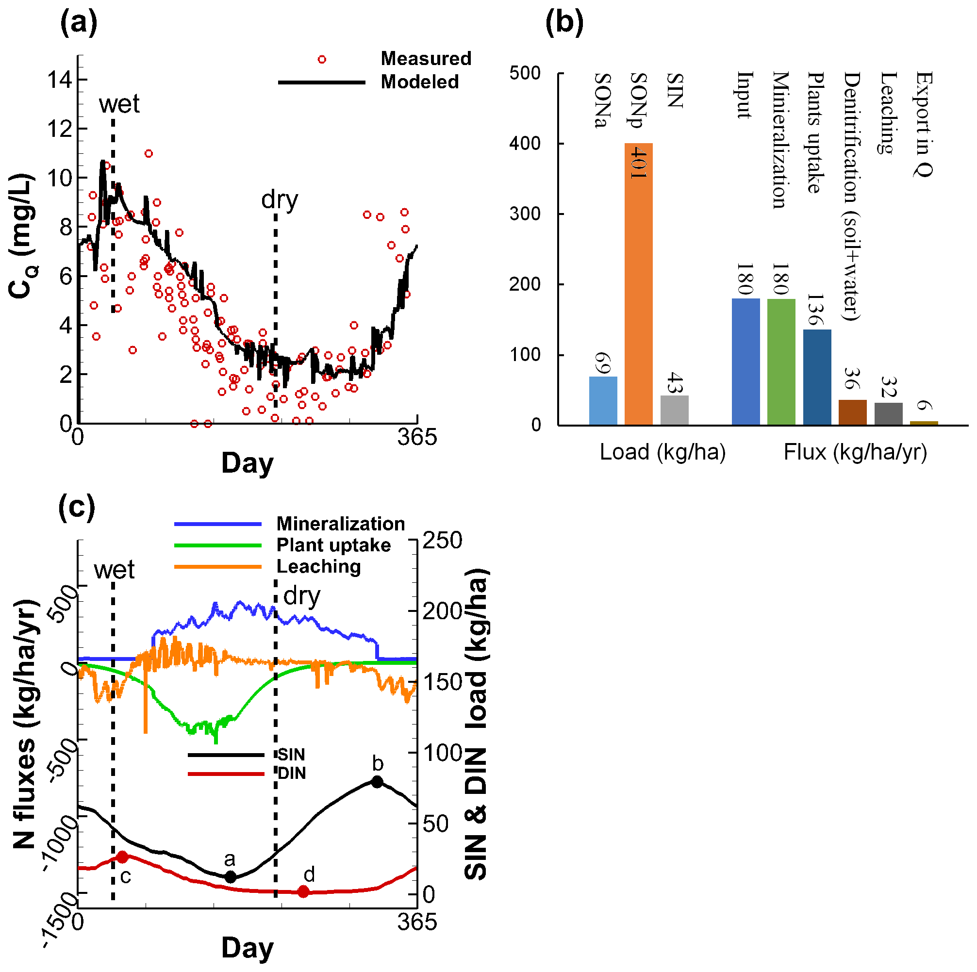
Figure 4 Simulated (a) in-stream nitrate concentration C_Q, (b) N loads and fluxes, and (c) time-variable N fluxes for the catchment of the base scenario. Note that the measured C_Q in (a) includes all the measurements from 2001 to 2010.

Figure 5 Comparing the monthly averaged C_Q with (a) the leaching flux and (b) the young water fractions of Q. The black lines are linear fits of the two variables, with r being the Spearman rank correlation coefficient. The numbers refer to the months.

4.2 Effect of topographic slope on flow

With the help of our simulations, it is possible to systematically explore the influence of topographic slope on the water flow and N fluxes. Figure 6 shows the responses of temporally-averaged Q and ET, the groundwater table depth, and flow weighted mean YF_Q and YF_ET to the changes of topographic slope. Under a constant climate, the changes of topographic slope can reshape the water flow via influencing flow partitioning between Q and ET. More water is taken up by ET and less water becomes Q in flatter landscapes (Fig. 6a). These patterns can be explained by the change of groundwater table depth (Fig. 6b), as shallower groundwater tables can be reached by the vegetation in flatter landscapes where ET therefore has a higher chance to remove water from the subsurface. The simulated YF_Q and YF_ET show generally increasing and decreasing patterns, respectively, when the topographic slope decreases (Fig. 6c), demonstrating that young streamflow is more prevalent in flatter landscape and young ET is more prevalent in steeper landscapes. However, the increasing pattern of YF_Q does not continue in steep catchments with slopes $>\mathrm{1}:\mathrm{60}$. Topographic slope changes YF_Q not only in terms of its mean value, but also in terms of its temporal variation. Figure 6d indicates that the maximum and minimum YF_Q are reached in February and August for the steepest catchment (slope 1:20), respectively, and in November and April for the flattest catchment (slope 1:1000).

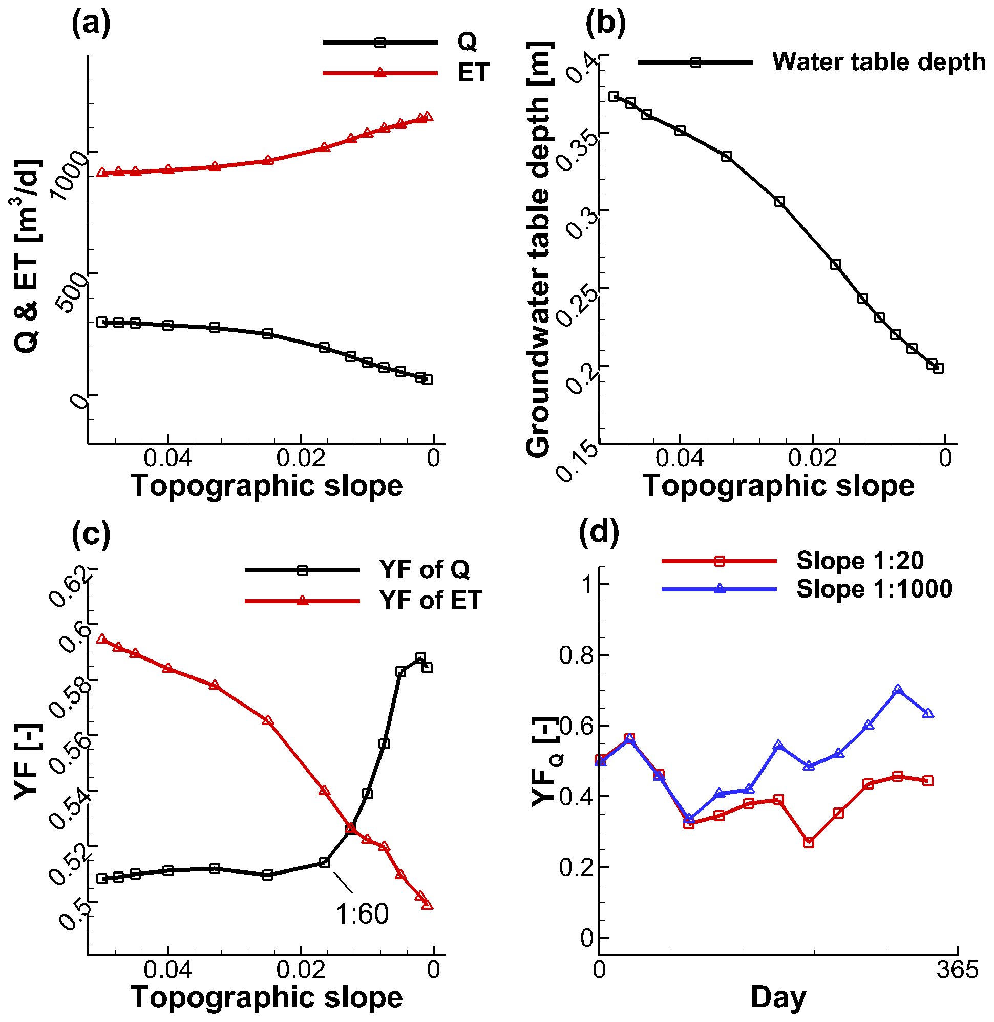
Figure 6 The simulated (a) Q and ET, (b) spatially-averaged depth of the groundwater table from the land surface, and (c) young water fraction in streamflow YF_Q and evapotranspiration YF_ET, in relation to the topographic slope for the simulated catchments. (d) Temporal variations of YF_Q for a steep landscape (slope 1:20) and a flat landscape (slope 1:1000).

Interpreting the response of the YF_Q to topographic slope mechanistically requires a closer look at the flow processes using a cross-sectional view. We plotted the subsurface flow fields for the wet season at a cross section of the catchments with slopes 1:20 and 1:1000 (Fig. 7).

Figure 7a reveals that the hillslope part of the catchment with a slope of 1:20 is largely unsaturated so that the flow paths in this area are characterized by vertical infiltration. In contrast, the valley bottom is fully saturated. Overall, 34 % of the subsurface domain is characterized by vertical flow (flow in 34 % of the total aquifer volume is more vertical than horizontal). For this scenario, two main discharge routes to the stream can be identified: (i) a fraction of the groundwater flows through the fully saturated zone and exits the aquifer to the stream, and (ii) another fraction exits the aquifer via seepage near to where the groundwater table intersects the land surface, indicated by a large exchange flux (from subsurface to surface, positive). The seepage represents a preferential flow path allowing for discharge via overland flow instead of discharge via the sub-surface with longer transit times. Note that both of the discharge routes provide the pathways for the rainfall falling on the top hillslope to reach the stream.

When the slope is reduced to 1:1000, the flow pattern experiences significant changes (Fig. 7b) compared to the catchment with a slope of 1:20. Several hydrologic studies have described two different flow systems in aquifers: (i) a recharge-limited system where the thickness of the unsaturated zone is sufficient to accommodate any water-table rise and thus the elevation of the groundwater table is limited by the recharge, and (ii) a topography-limited system where the groundwater table is close or connected to the land surface such that any fluctuation in groundwater table can result in considerable change in surface runoff (Werner and Simmons, 2009; Michael et al., 2013). In the selected cross sections, the steeper one (slope 1:20) is a partially topography-limited system (Fig. 7a) (the hillslope is recharge-limited while the valley bottom is topography-limited). The flat one (slope 1:1000) is transformed into a fully recharge-limited system (from Fig. 7b) due to the reduced hydraulic head gradients. This transformation leads to three main effects: (i) the seepage flow vanishes because the groundwater table disconnects from the land surface. The seepage route that would discharge water from the top of hillslope to the stream is cut off. (ii) The infiltration processes are weakened, indicated by the fact that the portion of subsurface domain characterized by vertical flow is reduced from 34 % to 18 %. (iii) Local flow cells are more likely to form, where water infiltrates to the aquifer and eventually exits the aquifer via ET rather than via flow to the stream (Fig. 7b, the local flow cells are more pronounced in the dry season, see Fig. S3b).

Because of the three aforementioned effects, the connectivity between the stream and the more distant hillslopes is significantly reduced. Precipitation falling farther from the stream has a lower chance to reach the stream and a higher change to be intercepted by ET on its way to the stream. The hillslope that used to generate old streamflow does not contribute to streamflow anymore. While precipitation water close to the stream has a higher chance to contribute to streamflow. We concluded that the increase of the YF_Q in flat landscapes is due to this reduction of the longer flow paths and the persistence of shorter flow paths, as indicated by the computed TTDs (Fig. 7c).

Figure 7 Cross-sectional view of saturation, flow paths, and exchange fluxes between the surface and the subsurface in the wet season (February) for catchments with topographic slope (a) 1:20, and (b) 1:1000. The cross section is marked in Fig. 1a. The black lines represent the flow paths. The red curves show exchange fluxes (along the cross-sectional profiles), positive values indicate seepage to the land surface and negative values indicate infiltration to the subsurface. (c) The computed cumulative TTDs for Q during the wet season (February), for the catchment with topographic slope of 1:20 and 1:1000.

In summary, we identified a generally increasing pattern of YF_Q in response to the decreasing topographic slope. When the landscape becomes flatter, the hydraulic head gradient as the main driving force changes the aquifer from a partially topography-limited system to a recharge-limited system that is more likely to form local flow cells.

4.3 Effect of topographic slope on N export

Simulated results show that the topographic slope can influence the N loads and fluxes in catchments. Figure 8a demonstrates that SIN tends to be higher in flatter and lower in steeper landscapes. This generally indicates that a flat landscape has a higher potential to retain N in the soil. However, the DIN is not significantly influenced by the topographic slope. N fluxes of leaching and export to the stream exhibit the opposite pattern. For the N fluxes, the leaching into groundwater decreases with the decrease of topographic slope (Fig. 8b). This is mainly because the flow velocity (influencing the leaching rate according to Eq. 6) in flatter landscape is lower due to the reduced hydraulic head gradient. Comparing the time-variable leaching between the steepest and flattest catchments (slope 1:20 and 1:1000, Fig. 8c), it can be observed that the leaching reduction in the flatter landscape mainly occurs in the wetting period (November to December). This may be because the response of flow velocity in the flatter catchment is not as large as that in the steeper catchment when the system transitions from dry to wet conditions. A large portion of the leached N mass has been degraded during transport in the groundwater, with the fraction rising from 80 % in the steepest landscape to 95 % in the flattest landscape (Fig. 8b). Mechanically, the reduced connectivity between the stream and more distant hillslopes in flatter landscapes inhibits the N export to the stream promoting the degradation by increasing the N residence time in the catchment. Subsequently, the N export shows a decreasing pattern with the decrease of topographic slope (Fig. 8b).

The calculated flow-weighted mean C_Q shows a decreasing trend in response to the decreasing topographic slope (Fig. 8d), from 7.3 mg L⁻¹ in the steepest catchment to 4.2 mg L⁻¹ in the flattest catchment. Even though both Q and N export show decreasing patterns with the decrease of topographic slope, the N export decreases to a higher degree than Q, indicated by the normalized values (Fig. 8e). Comparing the time-variable C_Q between the steepest and flattest catchments (slope 1:20 and 1:1000, Fig. 8f), it can be observed that the topographic slope influences the C_Q in two ways: (i) the C_Q is generally lower (but not always) in the flatter landscape over most of the time in a year, and (ii) the high peaks of C_Q in flatter landscapes are delayed in time. However, the high concentrations always occur in the wet periods (January–April) and low concentrations always occur in the dry periods (July–October).

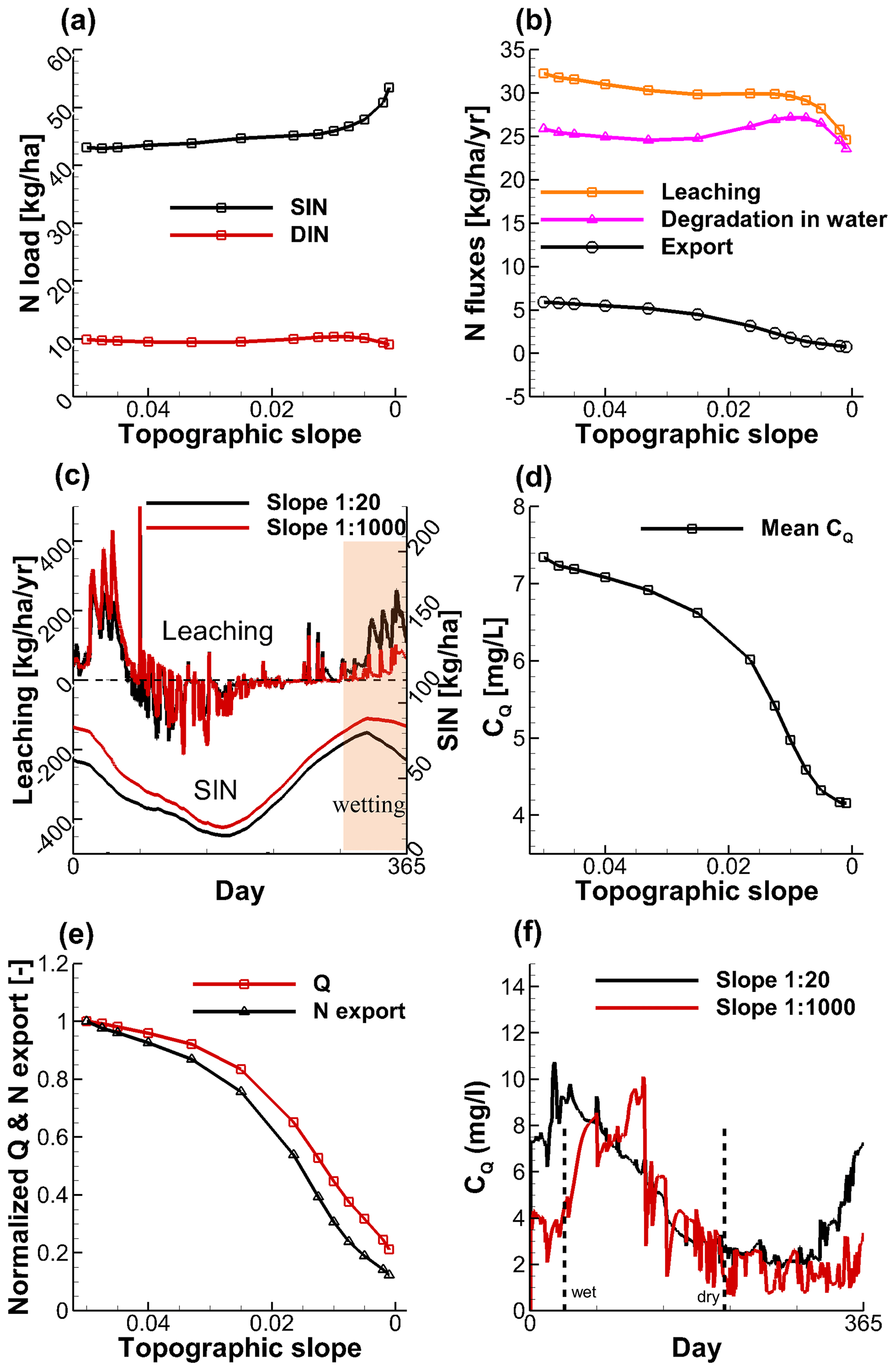
Figure 8 The simulated (a) N loads and (b) N fluxes in relation to the topographic slope for the simulated catchments. (c) Comparison of the time variable N loads and fluxes between a steep (slope 1:20) and a flat landscape (slope 1:1000). The simulated (d) flow-weighted mean C_Q, and (e) the normalized Q and N export (normalized to their values of the base scenario) in relation to the topographic slope. (f) Comparison of the time variable C_Q between a steep (slope 1:20) and a flat landscape (slope 1:1000). Note that for the leaching fluxes in (c), positive values are referred to as the N leaching from the soil to the groundwater, and negative values are referred to as the precipitation of N from groundwater to the soil by the evapoconcentration effect. The vertical dashed lines indicate the time when the catchment reaches the wettest (left) and the driest (right) conditions.

4.4 Discussion

Jasechko et al. (2016) reported that (the logarithm of) catchment topographic slope was significantly negatively correlated with young streamflow fractions with a Spearman rank correlation of −0.36. This conclusion was made statistically based on their observed 254 sites. Our numerical study based on the 11 catchments with different slopes but identical climate conditions resulted in more physically-based information that goes beyond such statistical correlations. Our results confirm that young streamflow fraction and slope generally exhibit a negative correlation. Additionally, our results show that the young water fraction in ET is positively correlated with the slope.

From the steepest landscape to the flattest landscape, catchments are likely to transition from a partially topography-limited flow system to a recharged limited system, due to the reduction of hydraulic gradient. The groundwater table is closer to the land surface when the landscape becomes flatter. The larger young streamflow fraction in flatter landscapes is consistent with the statement made by Jasechko et al. (2016) that the young streamflow fraction is more prevalent in flatter catchments which are characterized by more shallow lateral flow and less vertical infiltration. This phenomenon is also consistent with a negative correlation between groundwater table depth and young streamflow fraction, which has been frequently reported (Bishop et al., 2004; Seibert et al., 2009; Frei et al., 2010; Jasechko et al., 2016). Using the insight into the flow processes of the catchment, we found that the connectivity between the stream and the more distant hillslopes is reduced in flatter landscape, due to the reduced seepage flow, the weakened infiltration, and the formation of local flow cells that do not deliver flow to the stream. Our study points out that the reduction of this connectivity, which results in the reduction of the longer flow paths and the persistence of shorter flow paths, causes the increase of the young streamflow fraction.

Basically, the position of the groundwater table, flow path lengths, and flow velocities, which are all different for different topographic slopes, jointly affect the young streamflow fractions. Besides that, temporal variability of these three factors drives the distinct responses of the young streamflow fraction to topographic slope between seasons. In our simulated catchments, the negative correlation between young streamflow fraction and topographic slope is more pronounced in the flat landscapes with slopes $<\mathrm{1}:\mathrm{60}$. This demonstrates that the system is complex and apparently contains various threshold effects disturbing a straightforward monotonous relationship between catchment characteristics (e.g., slope) and young water fraction (or streamflow concentration). In this sense, systematically investigating the reaction of the flow dynamics to catchment characteristic is necessary, rather than assuming a straightforward cause–effect relationship that can be misleading.

Our results demonstrate that stream water quality is potentially less vulnerable in flatter landscapes. The flatter landscapes tend to retain more N mass in the soil and export less N mass to the stream. This behavior can be attributed to (i) the reduced leaching in flat landscapes since the decreased flow velocity physically reduces the potential of water to solve and transport the solute, and (ii) the increased potential of degradation because the connectivity between the stream and hillslope is blocked (i.e., there is more time for decay). Our results also show that higher C_Q is more prevalent in steeper landscapes. Note that this is concluded for average concentrations. Observations from the Selke Catchment, Central Germany, show that the C_Q is not always lower in flatter regions (Dupas et al., 2017; Nguyen et al., 2022). In the future more attention should be paid to the temporal variation and the timescale concerning the effect of topographic slope on C_Q. Additionally, our results show that we can expect lower C_Q and higher young streamflow fractions in flatter landscapes. This suggests that, with regard to the N transport in catchments, a large young streamflow fraction is not sufficient for high levels of C_Q. This phenomenon has not yet been reported to the best of our knowledge.

Concerning the seasonal variations of C_Q, our results showed that significant seasonal variation can be expected under temperate humid climates regardless of topographic slope. The high peak concentrations occurred in the wet and the low in the dry seasons, being consistent with the findings of previous studies (Benettin et al., 2015; Harman, 2015; Kim et al., 2016; Yang et al., 2018). However, the topographic slope can slightly shift the high peak concentrations in time.

4.5 Limitations and outlook

The cross-comparison between catchments with differing topographic slopes provides physically-based insights into the effects of topographic slope on nitrate export responses in terms of N fluxes and mean concentrations. However, this study is limited in scope in that it neglects other factors that may also have important impacts on the young streamflow and nitrate export processes:

• First, our study only considered the aquifers that are unconfined with an impermeable base and prescribed heterogeneity. Other catchment characteristics such as landscape aspect, catchment area, aquifer permeability or drainage ability, aquifer depth, stream bed elevation, fractured bedrock permeability, bedrock slope, and shape of basin can potentially change the flow patterns and age composition in streamflow (McGlynn et al., 2003; Broxton et al., 2009; Sayama and McDonnell, 2009; Stewart et al., 2010; Jasechko et al., 2016; Heidbüchel et al., 2013, 2020; Zarlenga and Fiori, 2020). For example, aquifers with high permeability or highly fractured bedrock are more likely to use deep rather than shallow flow paths and preferential discharge routes that lead to rapid drainage. Apart from that, it was reported that hydrological features such as precipitation variability, ET, and antecedent soil moisture are also significantly linked to transit times (Sprenger et al., 2016; Wilusz et al. 2017; Evaristo et al., 2019; Heidbüchel et al., 2013, 2020). For example, compared to uniform precipitation, event-scale precipitation is more likely to trigger rapid surface runoff and intermediate flow, such that the contribution of young water from storage to streamflow can be increased. Therefore, further research should consider a more complex model structure involving various heterogeneity and climate types.

• Second, several main simplifications were used in the formulation of the nitrate transport processes. (i) Transport modeling employed a constant degradation rate coefficient assuming that transit time was the only factor to determine degradation. This assumption neglected other factors that can spatially and temporally affect denitrification rates, such as temperature, redox boundaries (e.g., high oxygen concentration in shallow flow paths), and the amount of other nutrients (e.g., carbon), which also contribute to the seasonality in nitrate concentrations (Böhlke et al., 2007). Apart from that, we did not account for the long-term (decades, Van Meter et al., 2017) nitrate legacy effect as the dissolved nitrate in groundwater reservoirs degraded continuously in our model, which would not occur in older reservoirs where the denitrification is very slow or deactivated (e.g., due to the lack of a carbon source). (ii) The N external input source was uniformly applied across the land surface in our modeling. However, strong source heterogeneity may exist in catchments. For example, the N external input varies between land uses or along the soil profile (Zhi et al., 2019). This spatial source heterogeneity could affect the seasonal variations of C_Q (Musolff et al., 2017; Zhi et al., 2019) and should be considered in further research.

While the numerical model provided general insights, there was potential uncertainty in the simulated results. Firstly, the aforementioned simplifications may introduce model structural errors. Secondly, the model calibration was only constrained by limited data sets, which may lead to the non-uniqueness in the model parameters. Both of the aspects may introduce uncertainty in the simulated N loads and fluxes. Future work should be devoted to better constrain the model parameters, either by enhancing the concentration data quality through more frequent measurements or by providing additional data sets related to the N pool. Despite these limitations, the numerical experiments in this study could clearly identify the response of young streamflow and nitrate export to topographic slope under a humid seasonal climate, and show that hydraulic gradient is an important factor causing flow field differences between the catchments. This was achieved by using the advantages of a physically-based flow simulation that allows for a more mechanistic evaluation of flow processes, which would be impossible with a purely data-driven analysis based on, e.g., isotopic tracers only.

5 Conclusions

Previous data-driven studies suggested that catchment topographic slope impacts the age composition of streamflow and consequently the in-stream concentrations of certain solutes (Jasechko et al., 2016). We attempted to find more mechanistic explanations for these effects. We chose the small agricultural catchment “Schäfertal” in Central Germany, and based on it generated 11- synthetic catchments of varying topographic slope. The groundwater and overland flow, and the N transport in these catchments were simulated using a coupled surface–subsurface model. Water age compositions for Q and ET were determined using numerical tracer experiments. Based on the calculated flow patterns, young water fractions in streamflow YF_Q, N mass fluxes, and in-stream nitrate concentration C_Q, we systematically assessed the effects of varying catchment topographic slopes on the nitrate export dynamics in terms of the mass fluxes and annual mean concentration levels. The main conclusions of this study are the following:

• Under the considered humid climate, YF_Q is generally negatively correlated to topographic slope. When the landscape becomes flatter, the hydraulic head gradient is the main driving force to change the aquifer from a partially topography-limited system to a recharge-limited system, reducing the connectivity between the stream and the more distant hillslopes. This change results in the reduction of longer flow paths and the persistence of shorter flow paths, subsequently causing the flatter landscapes to generate younger streamflow.

• The flatter landscapes tend to retain more N mass in soil and export less N mass to the stream. These patterns are attributed to (i) the reduced leaching in flat landscape as the decreased flow velocity physically reduces the potential of water to transport the solute towards the stream, and (ii) the increased potential of degradation as the connectivity between the stream and hillslope is blocked and the solute stays inside the aquifer longer.

• For the considered catchment, the annual mean C_Q shows a decreasing trend in response to the decreasing topographic slope, because the N export decreases to a higher degree than Q. Flatter landscapes tend to generate larger young streamflow fractions (but lower C_Q), suggesting that a large young streamflow fraction is not sufficient for a high level of C_Q.

• Overall, this study provided a mechanistic perspective on how catchment topographic slope affects young streamflow fraction and nitrate export patterns. The use of a fully-coupled flow and transport model extended the approach to investigate the effects of catchment characteristics beyond the frequently used tracer data-driven analysis. It can be used for similar studies of other catchment characteristics and for other solutes. The results of this study improved the understanding of the effects of certain catchment characteristics on nitrate export dynamics with potential implications for the management of stream water quality and agricultural activity, in particular for catchments in temperate humid climate with pronounced seasonality. Given the limitations of this study, future work should be devoted to improve the degradation formulation, to investigate further catchment characteristics, and to consider various climate types.

Appendix A: Notation

t	(T) time
T	(T) age/transit time/residence time
J	(LT−1) precipitation
ET	(LT−1) evapotranspiration
Q	(LT−1) discharge/streamflow
pS	(–) age distribution of storage
$p_{\text{ET}/Q}$	(–) age distribution for evapotranspiration/
	discharge, equivalent to TTD
C	(M L−3) concentration
CQ	(M L−3) in-stream solute (nitrate) concentration
TQ	(M L−3) age (transit time) of discharge
YFQ	(–) young water fraction in streamflow, or young
	streamflow fraction
YFET	(–) young water fraction in ET
SON	(M L−2) soil organic nitrogen
SIN	(M L−2) soil inorganic nitrogen
DIN	(M L−2) dissolved inorganic nitrogen in water