the Creative Commons Attribution 4.0 License.
the Creative Commons Attribution 4.0 License.
 | 16 Sep 2022
Evaluation of water flux predictive models developed using eddy-covariance observations and machine learning: a meta-analysis
Haiyang Shi
Geping Luo
Olaf Hellwich
Mingjuan Xie
Chen Zhang
Yu Zhang
Yuangang Wang
Xiuliang Yuan
Xiaofei Ma
Wenqiang Zhang
Alishir Kurban
Philippe De Maeyer
Tim Van de Voorde
With the rapid accumulation of water flux observations from global eddy-covariance flux sites, many studies have used data-driven approaches to model water fluxes, with various predictors and machine learning algorithms used. However, it is unclear how various model features affect prediction accuracy. To fill this gap, we evaluated this issue based on records of 139 developed models collected from 32 such studies. Support vector machines (SVMs; average R-squared = 0.82) and RF (random forest; average R-squared = 0.81) outperformed other evaluated algorithms with sufficient sample size in both cross-study and intra-study (with the same data) comparisons. The average accuracy of the model applied to arid regions is higher than in other climate types. The average accuracy of the model was slightly lower for forest sites (average R-squared = 0.76) than for croplands and grasslands (average R-squared = 0.8 and 0.79) but higher than for shrubland sites (average R-squared = 0.67). Using , precipitation, Ta, and the fraction of absorbed photosynthetically active radiation (FAPAR) improved the model accuracy. The combined use of Ta and is very effective, especially in forests, while in grasslands the combination of Ws and is also effective. Random cross-validation showed higher model accuracy than spatial cross-validation and temporal cross-validation, but spatial cross-validation is more important in spatial extrapolation. The findings of this study are promising to guide future research on such machine-learning-based modeling.
- Article
(3139 KB) - Full-text XML
-
Supplement
(714 KB) - BibTeX
- EndNote


Evapotranspiration (ET) is one of the most important components of the water cycle in terrestrial ecosystems. It also represents the key variable in linking ecosystem functioning, carbon and climate feedback, agricultural management, and water resources (Fisher et al., 2017). The quantification of ET for regions, continents, or the globe can improve our understanding of water, heat, and carbon interactions, which is important for global change research (Xu et al., 2018). Information on ET has been used in many fields, including, but not limited to, droughts and heat waves (Miralles et al., 2014), regional water balance closures (Chen et al., 2014; Sahoo et al., 2011), agricultural management (Allen et al., 2011), water resources management (Anderson et al., 2012), and biodiversity patterns (Gaston, 2000). In addition, accurate large-scale and long-term time series ET prediction at high spatial and temporal resolution has been of great interest (Fisher et al., 2017).
Currently, there are three main approaches for simulation and spatial and temporal prediction of ET: (i) physical models based on remote sensing, such as surface energy balance models (Minacapilli et al., 2009; Wagle et al., 2017), the Penman–Monteith equation (Mu et al., 2011; Zhang et al., 2010), and the Priestley–Taylor equation (Miralles et al., 2011); (ii) process-based land surface models, biogeochemical models, and hydrological models (Barman et al., 2014; Pan et al., 2015; Sándor et al., 2016; Chen et al., 2019); and (iii) the observation-based machine learning modeling approach with in situ eddy-covariance (EC) observations of water flux (Jung et al., 2011; Li et al., 2018; Van Wijk and Bouten, 1999; Xie et al., 2021; Xu et al., 2018; Yang et al., 2006; Zhang et al., 2021). For remote-sensing-based physical models and process-based land surface models, some physical processes have not been well characterized due to the lack of understanding of the detailed mechanisms influencing ET under different environmental conditions. For example, the inaccurate representation and estimation of stomatal conductance (Li et al., 2019) and the linearization (McColl, 2020) of the Clausius–Clapeyron relation in the Penman–Monteith equation may introduce both empirical and conceptual errors into estimates of ET. Limited by complicated assumptions and model parametrizations, these process-based models face challenges in the accuracy of their ET estimations over heterogeneous landscapes (Pan et al., 2020; Zhang et al., 2021). Therefore, many researchers have used data-driven approaches for the simulation and prediction of ET with the accumulation of a large volume of measured observational data of water fluxes in the past decades. Various machine learning models have been developed to simulate water fluxes at the flux site scale. Further, various predictor variables (e.g., meteorological factors, vegetation conditions, and moisture supply conditions) have been incorporated into such models for upscaling (Fang et al., 2020; Jung et al., 2009) of water flux to a larger scale or understanding the driving mechanisms with the variable importance analysis performed in such models.
However, to date, the systematic assessment of the uncertainty in the processes of water flux prediction models constructed using the machine learning approach is limited. Although considerable effort has been invested in improving the accuracy of such prediction models, our understanding of the expected accuracy of such models under different conditions is still limited. It is still not easy for us to give the general guidelines for selecting appropriate predictor variables and models. Which predictor variables are the best in water flux simulations? How can the prediction accuracy of water flux effectively be improved? Such questions still confuse the researchers in the field. Therefore, we should synthesize the findings from published studies to determine which predictor variables, machine learning models, and other features can significantly improve the prediction accuracy of water flux. Also, we are interested in understanding under which specific conditions they are more effective.
A variety of features control the accuracy of such models, including the predictor variables used, the inherent heterogeneity within the dataset, the plant functional type (PFT) and characteristics of the flux sites, model construction and validation skills, and the algorithms used.
Predictor variables used. Compared to process-based models, the data used may have a more significant impact on the final model performance in data-driven models. Various biophysical covariates and other environmental factors have been used for the simulation and prediction of water fluxes. The most commonly used factors include mainly precipitation (P), air temperature (Ta), wind speed (Ws), net/sun radiation (), soil temperature (Ts), soil texture, vapor-pressure deficit (VPD), the fraction of absorbed photosynthetically active radiation (FAPAR), vegetation index (e.g., normalized difference vegetation index (NDVI), enhanced vegetation index (EVI)), leaf area index (LAI), and carbon fluxes (e.g., gross primary productivity (GPP)). These predictor variables used and their complex interactions drive the fluctuations and variability of water fluxes. They affect the accuracy of water flux simulations in two ways: their actual impact on water fluxes at the process-based level and their spatiotemporal resolution and inherent accuracy. The relationship between water fluxes and these variables at the process-based driving mechanism level is very different under different PFTs, different climate types, and different hydrometeorological conditions. For example, in irrigated croplands in arid regions, water fluxes may be highly correlated with irrigation practices, and thus soil moisture may be a very important predictor variable, and its importance may be significantly higher than in other PFTs. And in models that incorporate data from multiple PFTs, some variables that play important roles in multiple PFTs may have higher importance. In terms of data spatial and temporal resolution, the data for these predictor variables may have different scales. In terms of spatial resolution, meteorological observations such as precipitation and air temperature are at the flux site scale, while factors extracted from satellite remote sensing and reanalysis climate datasets cover a much larger spatial scale (i.e., the grid scale). This leads to considerable differences in the degree of spatial match between different variables and the site-scale EC observations (approximately 100 m × 100 m). It is therefore difficult for some variables to be fairly compared in the subsequent importance analysis of driving factors. In terms of temporal resolution, the importance of predictor variables with different temporal resolutions may be variable for models with different timescales (e.g., half-hourly, daily, and monthly models). For example, the daily or 8 d NDVI data based on MODIS satellite imagery may better capture the temporal dynamics of water fluxes concerning vegetation growth than the 16 d NDVI data derived from Landsat images. In addition, data on non-temporal dynamic variables such as soil texture cannot explain temporal variability in water fluxes in the data-driven simulations, although soil texture may be important in the interpretation of the actual driving mechanisms of ET (which may need to be quantified in detail in ET simulations by process-based models). In addition, some inherent accuracy issues (e.g., remote-sensing-based NDVI may not be effective at high values) of the predictors may propagate into the consequent machine learning models, thus affecting the modeling and our understanding of its importance. Therefore, it is necessary to consider the spatial and temporal resolution of the data and their inherent accuracy for the predictors used in different studies in the systematic evaluation of data-driven water flux simulations.
The heterogeneity of the dataset and model validation. The volume and inherent spatiotemporal heterogeneity of the training dataset (with more variability and extremes incorporated) may affect model accuracy. Typically, training data with larger regions, multiple sites, multiple PFTs, and longer year spans may have a higher degree of imbalance (Kaur et al., 2019; Van Hulse et al., 2007; Virkkala et al., 2021; Zeng et al., 2020). And in machine learning, in general, modeling with unbalanced data (with significant differences in the distribution between the training and validation sets) may result in lower model accuracy. Currently, the most common ways of model validation include spatial, temporal, and random cross-validation. Spatial validation is mainly to evaluate the ability of the model to be applied in different regions or flux sites with different PFT types, and one of the common methods is “leave one site out” (Fang et al., 2020; Papale et al., 2015; Zhang et al., 2021). If the data of the site left out for validation differ significantly from the distribution of the training dataset, the expected accuracy of the model applied at that site may be low because the trained model may not capture the specific and local relationships between the water flux and the various predictor variables at that site. For temporal validation, to assess the ability of the models to adapt to the interannual variability, typically some years of data are used for training and the remaining years for model validation (Lu and Zhuang, 2010). If a year with extreme climate is used for validation, the accuracy may be low because the training dataset may not contain such extreme climate conditions. In the case of PFTs that are significantly affected by human activities, such as cropland, the possible different crops grown and different land use practices (e.g., irrigation) across years can also lead to low accuracy in temporal validation.
Various machine learning algorithms. Some machine learning algorithms may have specific advantages when applied to model the relationships between water fluxes and covariates. For example, neural networks may have an advantage in nonlinear fitting, while random forests can avoid serious overfitting problems. However, which algorithm is better overall in different situations (i.e., applied to different datasets)? Which algorithm is generally more accurate than the others when using the same dataset? A comprehensive evaluation is important.
Therefore, to systematically and comprehensively assess the impact of various features in such modeling, we perform a meta-analysis of published water flux simulation studies that combine the flux site water flux observations, various predictors, and machine learning. The accuracy of model records collected from the literature was linked with various model features to assess the impacts of predictor data types, algorithms, and other features on model accuracy. The findings of this study may be promising to improve our understanding of the impact of various features of the models to guide future research on such machine-learning-based modeling.
2.1 Protocol for selecting the sample of articles
We applied a general query (on 1 December 2021) on title, abstract, and keywords to include articles with the “OR” operator applied among expressions (Table 1) in the Scopus database. Preferred Reporting Items for Systematic Reviews and Meta-Analyses (PRISMA) (Moher et al., 2009) are followed when filtering the papers. We first excluded articles that obviously did not fit the topic of this study based on the abstract and then performed the article screening with the full-text reading.
The inclusion of articles follows the following criteria:
- a.
Articles were filtered for those with water fluxes (or latent heat) simulated.
- b.
The water flux or latent heat observations used in the prediction models should be from the eddy-covariance flux measurements.
- c.
Articles focusing only on gap-filling (Hui et al., 2004) techniques (i.e., the objective was not simulation and extrapolation of water fluxes using machine learning) were excluded.
- d.
Only articles that used multivariate regression (with the number of covariates greater than or equal to 3) were included.
- e.
The determination coefficient (R-squared) of the validation step should be reported as the metric of model performance (Shi et al., 2021; Tramontana et al., 2016; Zeng et al., 2020) in the articles.
- f.
The articles should be published in English-language journals.
Although RMSE is also often used for model accuracy assessment, its dependence on the magnitude of water flux values makes it difficult to use for fair comparisons between studies. For example, due to the difference in the range of ET values, models developed from flux stations in dry grasslands will typically have lower RMSE than models developed by flux stations based on forests in humid regions. Therefore, RMSE may not be a good metric for cross-study comparisons in this meta-analysis.
Table 1Article search: “[A1 OR A2 OR A3…] AND [B1 OR B2 OR B3…] AND [C1 OR C2 OR C3 OR C4…]”.

2.2 Features of the prediction processes evaluated
The various features (Table 2) involved in the water flux modeling framework (Fig. 1) include the PFTs of the sites, the predictors used, the machine learning algorithms, the validation methods, and other features. Each model for which R-squared is reported is treated as a data record. If multiple algorithms were applied to the same dataset, then multiple records were extracted. Models using different data or features are also recorded as multiple records.

Figure 1Features of the machine-learning-based water flux prediction process. (a) The eddy-covariance-based water flux observations of various plant function types (PFTs), modified from (Paul-Limoges et al., 2020). ET – evapotranspiration. E – evaporation. T – transpiration. (b) Predictors and their spatial and temporal resolution. (c) The machine learning algorithms used for the modeling, such as neural networks and random forests. (d) The model validation methods used, including the spatial, temporal, and random cross-validations.
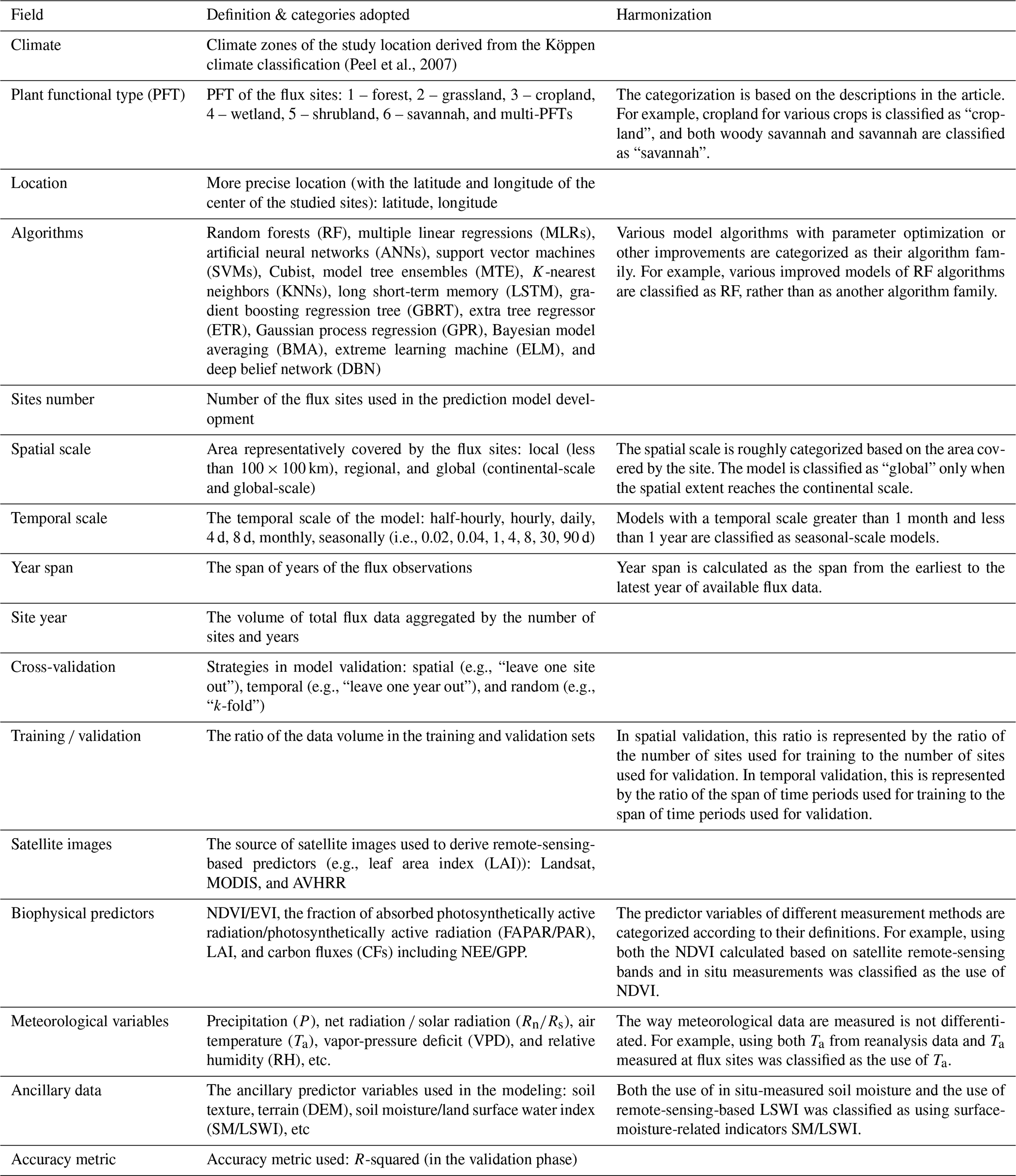
Table 2Model feature-related information collected from the papers included in this meta-analysis.
3.1 Articles included in the meta-analysis
A total of 32 articles (Table S1 in the Supplement) containing a total of 139 model records were included. The geographical scope of these articles was mainly Europe, North America, and China (Fig. 2).
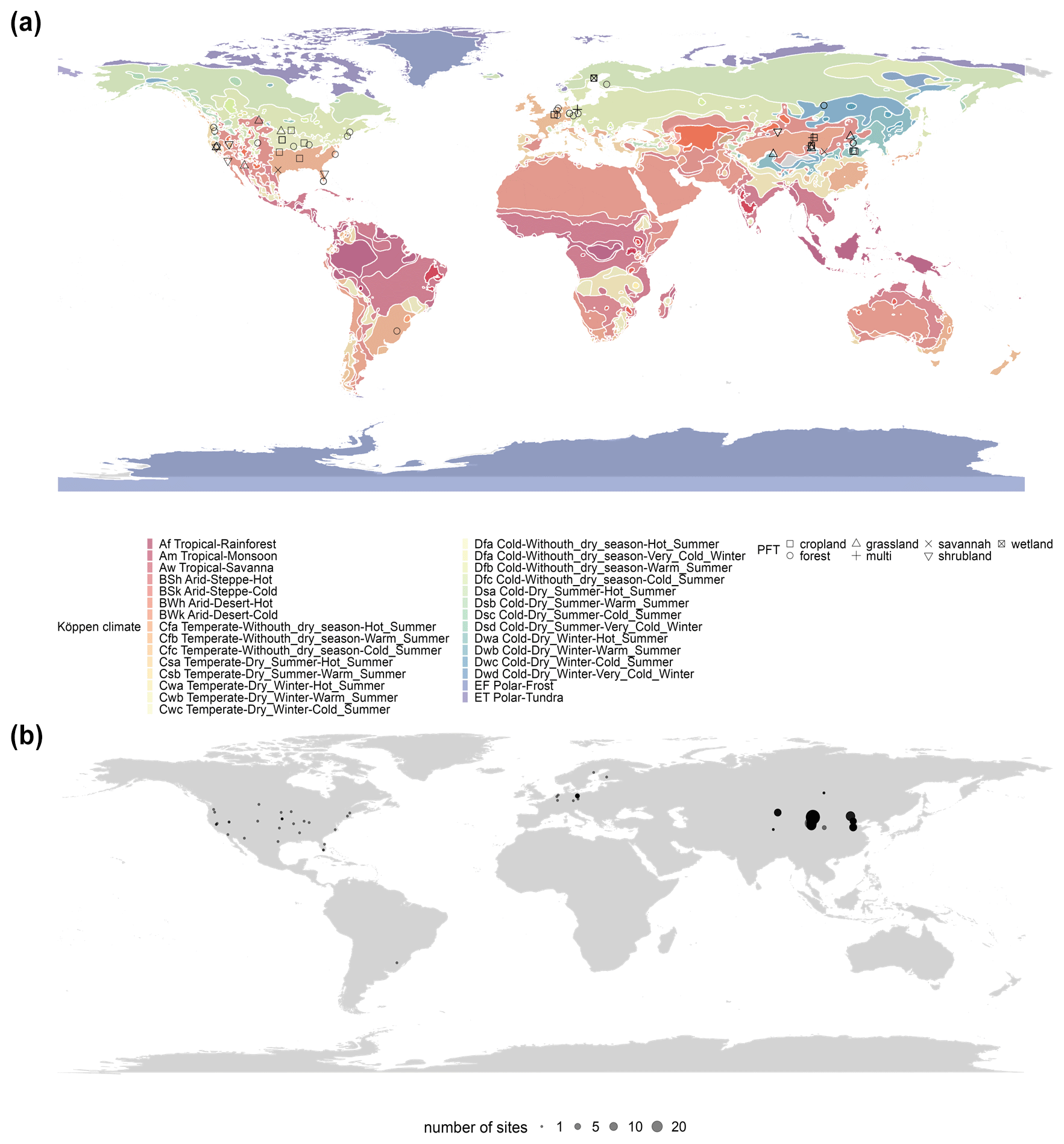
Figure 2Location of the included studies in the meta-analysis. (a) PFTs and the climate zones (from Köppen climate classification) of these studies and (b) the number of flux sites included in each study. Global- and continental-scale studies (e.g., models developed based on FLUXNET of the global scale) are not shown on the map due to the difficulty of identifying specific locations.
3.2 The formal meta-analysis
3.2.1 Algorithms
SVM and RF outperformed (Fig. 3a) other algorithms across studies (better than other algorithms with sufficient sample size in Fig. 3a such as ANN). These three machine learning algorithms (i.e., ANN, SVM, and RF) were significantly more accurate than the traditional MLR. Other algorithms such as MTE, ELM, and Cubist also have a high accuracy but with limited evidence sample size (Fig. 3a). In the internal comparison (different algorithms applied to the same dataset) in single studies, we also find that SVM and RF were slightly more accurate than ANN (Fig. 3b), and all these three (i.e., ANN, SVM, and RF) are considerably more accurate than MLR. Overall, SVM and RF have shown higher accuracy in water flux simulations in both inter- and intra-study comparisons with sufficient sample size as evidence.
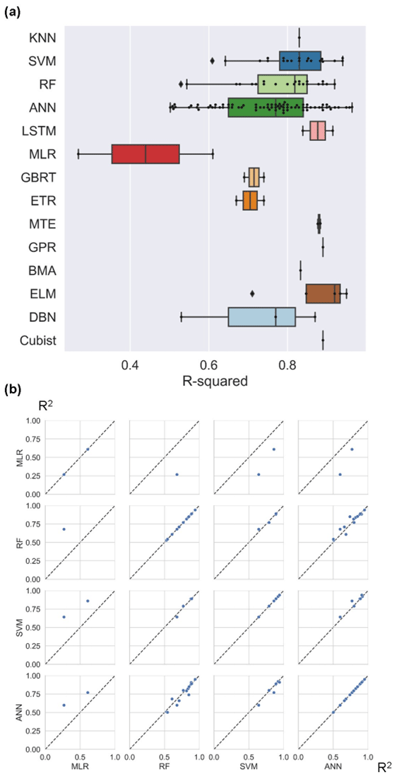
Figure 3Model accuracy (R-squared) using various algorithms across studies (a) and internal comparisons of selected pairs of algorithms within studies (b). Algorithms: random forests (RFs), multiple linear regressions (MLRs), artificial neural networks (ANNs), support vector machines (SVMs), Bayesian model averaging (BMA), Cubist, model tree ensembles (MTE), gradient boosting regression tree (GBRT), extra tree regressor (ETR), K-nearest neighbors (KNNs), long short-term memory (LSTM), Gaussian process regression (GPR), extreme learning machine (ELM), and deep belief network (DBN).
3.2.2 Climate types and PFTs
We found higher average model accuracy in arid climate zones (Fig. 4a), such as the cold semi-arid (steppe) climate (BSk) and cold desert climate (BWk). Most of these studies were located in northwest China and the western United States. It may be caused by the simpler relationship between water fluxes and biophysical covariates in arid regions. In arid zones, due to the high potential ET, the variability in the actual ET may be largely explained by water availability (moisture supply) and vegetation change, with the effect of variability in thermal conditions reduced. As for the various PFTs, the average model accuracy was slightly lower for forest types than for cropland and grassland types (Fig. 4b). The lowest average accuracy was found for shrub sites, which may be related to the difficulty of the remote-sensing-based vegetation index (e.g., NDVI) to quantify the physiological and ecological conditions of shrubs (Zeng et al., 2022), and the heterogeneity of the spatial distribution of shrubs within the EC observation area may also cause difficulties in capturing their relationships with biophysical variables. We also found high model accuracy for the wetland type, although records as evidence to support this finding may be limited. Compared to other PFTs, the more steady and adequate water availability in the wetland type may make the variations of water fluxes less explained by other biophysical covariates.
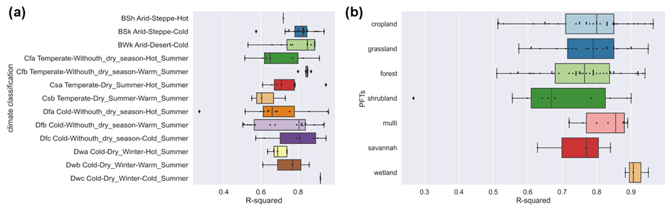
Figure 4Differences in model accuracy (R-squared) of (a) various climate zones (classified by Köppen climate classification) across studies and (b) PFTs. BSh – hot semi-arid (steppe) climate. BSk – cold semi-arid (steppe) climate. BWk – cold desert climate. Cfa – humid subtropical climate. Cfb – temperate oceanic climate. Csa – hot-summer Mediterranean climate. Csb – warm-summer Mediterranean climate. Dfa – hot-summer humid continental climate. Dfb – warm-summer humid continental climate. Dfc –subarctic climate. Dwa – monsoon-influenced hot-summer humid continental climate. Dwb – monsoon-influenced warm-summer humid continental climate. Dwc – monsoon-influenced subarctic climate.
3.2.3 Predictors and their combinations
On the one hand, for the effects of individual predictors, the use of , P, Ta, and FAPAR improved the accuracy of the model (Fig. S1 in the Supplement). This pattern partially changed in the different PFTs. In the forest sites, the accuracy of the models with and Ta used was higher than that of the models with and Ta not used. For the grassland sites, the use of Ws, FAPAR, P, and improved the model accuracy. For the cropland sites, Ta and FAPAR were more important for improving the model accuracy.
On the other hand, the evaluation of the effect of individual predictors on model accuracy is not necessarily reliable because some predictor variables are used together (e.g., the high model accuracy corresponding to a particular variable may be because it is often used together with another variable that plays the dominant role in improving accuracy). Therefore, we tested for independence between the use of variables and assessed the effect of the combination of variables on model accuracy. We calculated the correlation matrix (Fig. S2) between the use of various predictors (not used is set as 0, and used is set as 1). We found there was a dependence between the use of some predictors; the use of NDVI/EVI, LAI, and SM was significantly negatively correlated with the use of and Ta (Fig. S2). It indicated that many of the models that used and Ta did not use NDVI/EVI, LAI, and SM, and the models that used NDVI/EVI, LAI, and SM also happened not to use and Ta. Given this dependence, we evaluated the effect of the combination of variables on the model accuracy (Fig. 5). In Fig. 5, the three variable combinations on the left side are mainly meteorological variables, while the three variable combinations on the right side are mainly vegetation-related variables based on remote sensing (e.g., NDVI, EVI, LAI, and LSWI). We found that, overall, the accuracy of the models using only meteorological variable combinations was higher than that of the models using only remote-sensing-based vegetation-related variables. It demonstrated the importance of using meteorological variables in machine-learning-based ET prediction (probably especially for models with small timescales such as hourly scale, and daily scale). For example, in the forest type, the combination of Ta and is very effective compared to using only remote-sensing-based vegetation index variable combinations. The combination of Ta and is also effective in the grassland and cropland types. The combination of Ws and played an important role in the grassland type for improving model accuracy. Despite this, it does not negate the positive role of remote-sensing-based vegetation-related variables in ET prediction. This effectiveness can be dependent on the timescale of the model as well as the PFTs. In models with large timescales (monthly scale, seasonal scale) and PFTs in which ET is sensitive to vegetation dynamics, remote-sensing-based vegetation-related variables may also be of high importance.

Figure 5Effects of combinations of predictor variables on model accuracy in various PFTs (all data, forest, grassland, and cropland). Dark blue boxes indicate that the predictors were used together in the model (e.g., for “Ta & ”, the dark blue box represents Ta and were together used in the model), while dark red boxes indicate the other conditions (i.e., the combination was not used). Predictors: precipitation (P), soil moisture/remote-sensing-based land surface water index (SM), net radiation solar radiation (), enhanced vegetation index (EVI), air temperature (Ta), leaf area index (LAI), and normalized difference vegetation index/enhanced vegetation index (NDVI/EVI).
3.2.4 Other model features
We also evaluated the impact of some other features on accuracy. The differences in the accuracy of models with different spatial scales, year spans, number of sites, and volume of data (Fig. 6) appear to be insignificant. This seems to be related to the fact that in large-scale water flux simulations, the sites of similar PFTs are selected such as for modeling multiple forest sites across Europe (Van Wijk and Bouten, 1999) which focus on “forest” and multiple grassland sites across arid northern China (Xie et al., 2021; Zhang et al., 2021) which focus on “grassland”, rather than mixing different PFT types to train models as is done in machine learning modeling of carbon fluxes (Zeng et al., 2020). In terms of the timescales of the models, the 4 d, 8 d, and monthly scales appear to correspond to higher accuracy compared to the half-hourly and daily scales. The higher the ratio of the volume of data in the training and validation sets, the higher the model accuracy. Compared to the models using Landsat data, the models using MODIS data showed slightly higher accuracy probably due to the advantage of MODIS data in capturing the temporal dynamics of biophysical covariates. There were significant differences in the accuracy of the models using different cross-validation methods, with the models using random cross-validation showing higher accuracy than those using temporal cross-validation. This suggests that interannual variability may have a high impact on the models in water flux simulations. The driving mechanism of ET may vary significantly across years, and the inclusion of some extreme climatic conditions in the training set may be important for model accuracy and robustness.
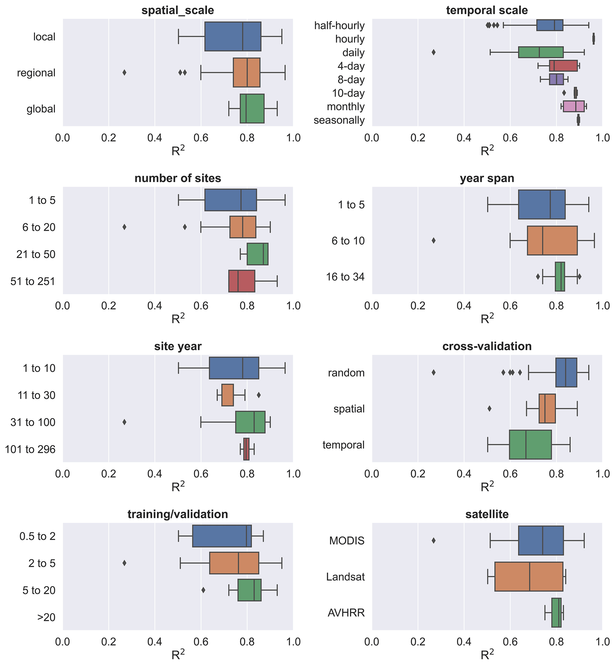
Figure 6The effects of other model features (i.e., spatial scale, number of sites, temporal scale, year span, site year, validation method, training validation ratio, and satellite imagery used) on the R-squared.
3.2.5 Linear correlation of quantitative features and R-squared
We also analyzed the linear correlation (Fig. 7) between multiple quantitative features and the R-squared. We found that the magnitude of the linear correlation coefficients between the use of predictor combinations and the R-squared was higher than other features. The use of the predictor combination Ta and significantly improved the model accuracy. Temporal scale, time span, training validation ratio, and number of sites showed weak positive correlations with R-squared (not significant, p value <0.1). The positive correlation between temporal scale and R-squared is higher among these features, although it is not significant. It should also be paid more attention to in future studies. The features training validation ratio and time span are also positively correlated (although not significantly) with the R-squared, suggesting the importance of the volume of data in the training set in a data-driven machine learning model. A larger training validation ratio and time span may correspond to greater proportional coverage of the scenarios/conditions in the training set over the validation set, and thus correspond to higher accuracy.
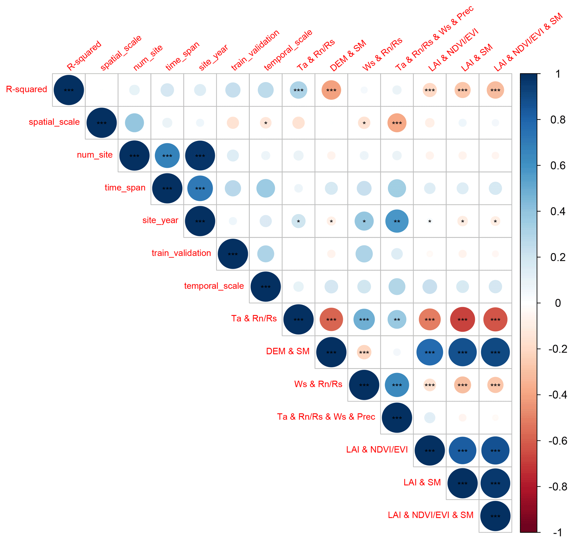
Figure 7Evaluation of linear correlations between multiple features and the R-squared records with the statistical significance test. For the spatial scale feature , the local scale was set to 1, the regional scale was set to 2, and the global scale was set to 3 in the analysis of linear correlation. For the use of various predictor combinations with “&”, the value for “used together ” is set as 1, and other conditions are set as 0 (e.g., for the Ta & & Ws & P feature, if Ta, , Ws, and P were used together in the model, the value is set as 1). Significance: the p value < 0.01 (), 0.05 (), and 0.1 (∗).
With the accumulation of in situ EC observations around the world, the study of ET simulations based on data-driven approaches has received more attention from researchers in the last decade. Many studies have combined EC observations, various predictors, and machine learning algorithms to improve the prediction accuracy of water fluxes. To date, the results of these studies have not been comprehensively evaluated to provide clear guidance for feature selection in water flux prediction models. To better understand the approach and guide future research, we performed a meta-analysis of such studies. Machine-learning-based water flux simulations and predictions still suffer from high uncertainty. By investigating the expected improvements that can be achieved by incorporating different features, we can avoid practices that may reduce model accuracy in future research.
4.1 Opportunities and challenges in the water flux simulation
In the above meta-analysis of the models, we found that water flux simulations based on EC observations can achieve high accuracy but also have high uncertainty through the modeling workflow. The R-squared of many water flux simulation models exceeds 0.8, possibly higher than some remote-sensing-based and process-based models and possibly higher than carbon flux simulations such as the net ecosystem exchange (NEE) in a similar modeling framework (Shi et al., 2022). This may be because many data on important variables affecting carbon flux such as soil and biomass pools, disturbances, ecosystem age, management activities, and land use history are not yet effectively and continuously measured (Jung et al., 2011) with the global spatially and temporally explicit information. While ET simulations rely on observations of moisture and energy conditions and vegetation conditions, many of the current available meteorological and remote-sensing data have been effective to represent and capture the spatial and temporal dynamics of these predictors well.
4.1.1 Comprehensive insights on model features
Biophysical and meteorological variables are both considered important in ET simulations. This study found that models using a combination of meteorological variables had higher accuracy than models using only remotely sensed vegetation dynamic information. However, due to the high proportion of models with small temporal scales (e.g., half-hourly scale, hourly scale, and daily scale) in this study, this advantage of the combination of meteorological variables may be more suitable for small temporal scales. A possible explanation is that vegetation-related variables such as NDVI and LAI at the daily scale, 8 d scale, and 16 d scale have limited explanatory ability for hourly or daily-scale variability in ET, especially under cloudy conditions (e.g., tropical rainforest regions); the temporal continuity of the vegetation index data may be greatly limited (Zeng et al., 2022). This should be given more attention, and some vegetation indices derived from hourly temporal resolution satellite remote-sensing data such as GOES (Zeng et al., 2022) can be used for ET simulations to investigate the possible added value of vegetation indices at smaller timescales. In contrast, at a small temporal scale, the use of combinations of meteorological variables can capture moisture and energy conditions that control the rapid fluctuations of ET and thus has a dominant role in hourly or daily-scale ET prediction. This also corroborates the high accuracy of some physic-based ET estimation models (Rigden and Salvucci, 2015) that use only meteorological variables and not vegetation-related variables such as NDVI (only an estimate of vegetation height derived from land cover maps is used to represent vegetation conditions; Rigden and Salvucci, 2015).
There are differences in model accuracy among different PFTs. For example, in forest sites, limitations in data accuracy of factors were possible because some remote-sensing-based predictors such as NDVI, FAPAR, and LAI have limited accuracy when applied to forest types (Liu et al., 2018b; Zeng et al., 2022). In addition, factors such as crown density, which may significantly affect the proportion of soil evaporation, transpiration, and evaporation of canopy interception, were not considered in these models, which may also lead to low model accuracy. This suggests that in water flux simulation, the driving mechanisms of water fluxes in different PFTs do affect the accuracy of machine learning models, and we need to consider more the actual and specific influencing factors in specific PFTs. More variables that can quantify the ratio of evaporation and transpiration should be considered for inclusion, which also appears to improve the mechanistic interpretability of such machine learning models. A previous study (Zhao et al., 2019) combined the physics-based approach (e.g., Penman–Monteith equation) and machine learning to build hybrid models to improve interpretability. We should make full use of empirical knowledge and experiences from process-based models to improve the accuracy and interpretability of the machine learning approach.
Among the validation methods, random cross-validation has higher accuracy than spatial cross-validation and temporal cross-validation. However, spatial cross-validation and temporal cross-validation may be able to better help us recognize the robustness of the model when extrapolated (i.e., applied to new stations and new years). The lower accuracy in the temporal cross-validation approach implies that we need to focus on interannual hydrological and meteorological variability in the water flux simulations. In cropland sites, we may also need to pay more attention to the effects of interannual variability in anthropogenic cropping patterns. If some extreme weather years are not included, the robustness of the model when extrapolated to other years may be challenged, especially in the context of the various extreme weather events of recent years. This can also inform the siting of future flux stations. Regions where climate extremes may occur and biogeographic types not covered by existing flux observation networks should be given more attention to achieve global-scale, accurate, and robust machine-learning-based spatiotemporal prediction of water fluxes. Furthermore, although the R-squared and the training validation ratio show a positive correlation (Fig. 7) (i.e., a higher training validation ratio may correspond to a higher R-squared), we should still be cautious in reducing this ratio in our modeling. For a really small validation set, it would be very challenging to determine which model is better given the potential uncertainty caused by the considerable randomness.
4.1.2 Differences from NEE predictions in the similar model framework
In general, predictors related to meteorological, vegetation, and soil conditions were common to both ET and NEE simulations in a similar framework (Shi et al., 2022). However, in NEE predictions, explanatory variables such as soil organic content, photosynthetic photon flux density, and growing degree days (Shi et al., 2022) are not necessary for ET predictions. The selection of these variables requires our prior knowledge of the dominant drivers of ET and NEE anomalies of particular ecosystems and their differences.
The accuracy of NEE predictions (Shi et al., 2022) can be more limited by global variability across biomes and locations (Nemani et al., 2003) given the lack of locally measured data on soil and biomass pools, disturbances, ecosystem age, management activities, and land use history (Jung et al., 2011). It can result in a higher heterogeneity of the training data in large-scale modeling with multiple flux sites (Shi et al., 2022) and the weak ability to capture the NEE anomalies. In contrast, in ET predictions, meteorological variables and vegetation conditions appear to be already sufficient to capture a considerably large fraction of the ET variations in most conditions.
In future ET prediction studies, given that few current ET products have timescales smaller than the daily scale (Jung et al., 2019; Pan et al., 2020), improvements in the accuracy of daily and hourly models may be necessary to fill this gap. In addition, the partitioning of ET components (i.e., transpiration, interception evaporation, and soil evaporation) can be more focused to better decouple the contributions of vegetation and soil to ET with machine learning (Eichelmann et al., 2022). It can be further matched with the partitioning of NEE (i.e., to GPP and ecosystem respiration) to increase our knowledge of the global water cycle and ecosystem functioning and obtain further refined global carbon–water fluxes coupling relations (Eichelmann et al., 2022). Also, the above two promising improvements can be beneficial for research on topics related to the global terrestrial water cycle (Fisher et al., 2017).
4.2 Uncertainties and limitations of this meta-analysis
4.2.1 The limited number of available literature and model records
Despite many articles and model records collected through our efforts to perform this meta-analysis, there still appears to be a long way to go to finally and completely understand the various mechanisms involved in water flux simulation with machine learning. Some of the insights provided by this study can not be robust (due to the limited sample size available when the goal is to assess the effects of multiple features), but this does not negate the fact that this study does obtain some meaningful findings. Therefore, researchers should treat the results of this study with caution, as they were obtained only statistically. Overall, it is still positive to conduct a meta-analysis of such studies, considering their rapid growth in the number and lack of guiding directions.
4.2.2 Publication bias and weighting
In a meta-analysis in other fields, weights for different studies can be assigned based on the quality of the journal and the extent to which the research data are publicly available (Borenstein et al., 2011; Field and Gillett, 2010). However, most of the articles included in this study did not fully publish the flux data they used, the models they developed, and the predicted ET data. Given this limitation, we were unable to assign them small weights due to the relatively limited available sample size of this study. Further, in meta-analyses in other fields, the sample size and the variance of the results of the experiments can also be used to adjust the weights of the effects among studies (Adams et al., 1997; Don et al., 2011; Liu et al., 2018a). However, for this study, due to the lack of a convincing way to determine the weights, we briefly assigned equal weight values to all the included studies.
4.2.3 Uncertainties in the information of the extracted features
At the information extraction level, the issues detailed here may also introduce uncertainties. Uncertainties caused by data quality control (e.g., gap-filling (Hui et al., 2004)) are difficult to assess effectively. Gap-filling is a commonly used technique to fill in low-quality data in flux observations. However, the impact of this practice on machine-learning-based ET prediction models is unclear, due to the difficulty of directly assessing how this technique is performed in various studies by this meta-analysis. Typically, models with small timescales (e.g., hourly scale and daily scale) can exclude low-quality observations and use only high-quality data. However, for models with large timescales (e.g., monthly scales), gap-filling (e.g., based on meteorological data) may be unavoidable. This may lead to a decrease in training data purity and introduce uncertainty in the subsequent prediction model development.
Systematic uncertainties caused by the energy balance closure (EBC) issue in eddy-covariance flux measurements are also difficult to assess by this meta-analysis. EBC is a common problem (Eshonkulov et al., 2019) in eddy-covariance flux observations. For that reason, the latent heat flux measured potentially underestimates ET. Some prediction models corrected EBC (e.g., using Bowen ratio preserving (Mauder et al., 2013, 2018) and energy balance residuals (Charuchittipan et al., 2014; Mauder et al., 2018)) in the processing of training data, but some did not. How this will affect the accuracy of the prediction model is not clear due to multiple factors that need to be evaluated that influence EBC (Foken, 2008), including measurement errors of the energy balance components, incorrect sensor configurations, influences of heterogeneous canopy height, unconsidered energy storage terms in the soil–plant–atmosphere system, inadequate time averaging intervals, and longwave eddies (Jacobs et al., 2008; Foken, 2008; Eshonkulov et al., 2019). To reduce this uncertainty, more attention to flux site characteristics (Eshonkulov et al., 2019) related to PFT, topography, flux footprint area, etc., to select the appropriate correction method is necessary for future studies.
As most studies used far more water flux observation records than the number of covariates in their regression models, we did not adjust the R-squared in this study to an adjusted R-squared.
The various specific ways in which the parameters of the model are optimized are not differentiated. They are broadly categorized into different families or kinds of algorithms, which may also introduce uncertainty into the assessment.
The assessment of some features is not detailed due to the limitations of the available model records. For example, the classification of PFT could be more detailed. “Forest” could be further classified as broadleaf forest and coniferous forest, etc., while “cropland” could be further classified as rainfed and irrigated cropland based on differences in their response mechanisms of water fluxes to environmental factors.
We performed a meta-analysis of the water flux simulation studies which focus on using machine learning approaches to combine flux station observations from flux stations/networks, meteorological, biophysical, and other ancillary predictors. The main conclusions are as follows:
-
SVM (average R-squared = 0.82) and RF (average R-squared = 0.81) outperformed over evaluated algorithms with sufficient sample size in both cross-study and intra-study (with the same training dataset) comparisons.
-
The average accuracy of the model applied to arid regions is higher than in other climate types.
-
The average accuracy of the model was slightly lower for forest sites (average R-squared = 0.76) than for cropland and grassland sites (average R-squared = 0.8 and 0.79) but higher than for shrub sites (average R-squared = 0.67).
-
Among various predictor variables, the use of , P, Ta, and FAPAR improved the model accuracy. The combination of Ta and is very effective, especially in the forest type, while in the grassland type, the combination of Ws and is also effective.
-
Among the different validation methods, random cross-validation shows higher model accuracy than spatial cross-validation and temporal cross-validation.
The code and data used in this study can be accessed by contacting the first author (shihaiyang16@mails.ucas.ac.cn).
The supplement related to this article is available online at: https://doi.org/10.5194/hess-26-4603-2022-supplement.
HS and GL were responsible for the conceptualization, methodology, formal analysis, investigation, visualization, and writing. OH contributed to the investigation. XM, XY, YW, WZ, MX, CZ, and YZ processed the data. AK, TVDV, and PDM provided supervision.
The contact author has declared that none of the authors has any competing interests.
Publisher's note: Copernicus Publications remains neutral with regard to jurisdictional claims in published maps and institutional affiliations.
We thank the editor and two anonymous reviewers for their insightful comments, which contributed substantially to the improvement of this paper.
This research has been supported by the National Natural Science Foundation
of China (grant no. U1803243), the Key Projects of the Natural Science
Foundation of Xinjiang Autonomous Region (grant no. 2022D01D01), the
Strategic Priority Research Program of the Chinese Academy of Sciences
(grant no. XDA20060302), and the High-End Foreign Experts project of China..
This open-access publication was funded by Technische Universität Berlin.
This paper was edited by Efrat Morin and reviewed by two anonymous referees.
Adams, D. C., Gurevitch, J., and Rosenberg, M. S.: Resampling tests for meta of ecological data, Ecology, 78, 1277–1283, 1997.
Allen, R. G., Pereira, L. S., Howell, T. A., and Jensen, M. E.: Evapotranspiration information reporting: I. Factors governing measurement accuracy, Agr. Water Manage., 98, 899–920, https://doi.org/10.1016/j.agwat.2010.12.015, 2011.
Anderson, M. C., Allen, R. G., Morse, A., and Kustas, W. P.: Use of Landsat thermal imagery in monitoring evapotranspiration and managing water resources, Remote Sens. Environ., 122, 50–65, https://doi.org/10.1016/j.rse.2011.08.025, 2012.
Barman, R., Jain, A. K., and Liang, M.: Climate-driven uncertainties in modeling terrestrial energy and water fluxes: a site-level to global-scale analysis, Global Change Biol., 20, 1885–1900, https://doi.org/10.1111/gcb.12473, 2014.
Borenstein, M., Hedges, L. V., Higgins, J. P., and Rothstein, H. R.: Introduction to meta-analysis, John Wiley & Sons, https://doi.org/10.1002/9780470743386, 2011.
Charuchittipan, D., Babel, W., Mauder, M., Leps, J.-P., and Foken, T.: Extension of the Averaging Time in Eddy-Covariance Measurements and Its Effect on the Energy Balance Closure, Bound.-Lay. Meteorol., 152, 303–327, https://doi.org/10.1007/s10546-014-9922-6, 2014.
Chen, Y., Xia, J., Liang, S., Feng, J., Fisher, J. B., Li, X., Li, X., Liu, S., Ma, Z., Miyata, A., Mu, Q., Sun, L., Tang, J., Wang, K., Wen, J., Xue, Y., Yu, G., Zha, T., Zhang, L., Zhang, Q., Zhao, T., Zhao, L., and Yuan, W.: Comparison of satellite-based evapotranspiration models over terrestrial ecosystems in China, Remote Sens. Environ., 140, 279–293, https://doi.org/10.1016/j.rse.2013.08.045, 2014.
Chen, Y., Wang, S., Ren, Z., Huang, J., Wang, X., Liu, S., Deng, H., and Lin, W.: Increased evapotranspiration from land cover changes intensified water crisis in an arid river basin in northwest China, J. Hydrol., 574, 383–397, https://doi.org/10.1016/j.jhydrol.2019.04.045, 2019.
Don, A., Schumacher, J., and Freibauer, A.: Impact of tropical land-use change on soil organic carbon stocks – a meta-analysis, Global Change Biol., 17, 1658–1670, https://doi.org/10.1111/j.1365-2486.2010.02336.x, 2011.
Eichelmann, E., Mantoani, M. C., Chamberlain, S. D., Hemes, K. S., Oikawa, P. Y., Szutu, D., Valach, A., Verfaillie, J., and Baldocchi, D. D.: A novel approach to partitioning evapotranspiration into evaporation and transpiration in flooded ecosystems, Global Change Biol., 28, 990–1007, https://doi.org/10.1111/gcb.15974, 2022.
Eshonkulov, R., Poyda, A., Ingwersen, J., Wizemann, H.-D., Weber, T. K. D., Kremer, P., Högy, P., Pulatov, A., and Streck, T.: Evaluating multi-year, multi-site data on the energy balance closure of eddy-covariance flux measurements at cropland sites in southwestern Germany, Biogeosciences, 16, 521–540, https://doi.org/10.5194/bg-16-521-2019, 2019.
Fang, B., Lei, H., Zhang, Y., Quan, Q., and Yang, D.: Spatio-temporal patterns of evapotranspiration based on upscaling eddy covariance measurements in the dryland of the North China Plain, Agr. Forest Meteorol., 281, 107844, https://doi.org/10.1016/j.agrformet.2019.107844, 2020.
Field, A. P. and Gillett, R.: How to do a meta, British J. Math. Stat. Psychol., 63, 665–694, 2010.
Fisher, J. B., Melton, F., Middleton, E., Hain, C., Anderson, M., Allen, R., McCabe, M. F., Hook, S., Baldocchi, D., Townsend, P. A., Kilic, A., Tu, K., Miralles, D. D., Perret, J., Lagouarde, J.-P., Waliser, D., Purdy, A. J., French, A., Schimel, D., Famiglietti, J. S., Stephens, G., and Wood, E. F.: The future of evapotranspiration: Global requirements for ecosystem functioning, carbon and climate feedbacks, agricultural management, and water resources, Water Resour. Res., 53, 2618–2626, https://doi.org/10.1002/2016WR020175, 2017.
Foken, T.: The energy balance closure problem: An overview, Ecol. Appl., 18, 1351–1367, 2008.
Gaston, K. J.: Global patterns in biodiversity, Nature, 405, 220–227, https://doi.org/10.1038/35012228, 2000.
Hui, D., Wan, S., Su, B., Katul, G., Monson, R., and Luo, Y.: Gap-filling missing data in eddy covariance measurements using multiple imputation (MI) for annual estimations, Agr. Forest Meteorol., 121, 93–111, https://doi.org/10.1016/S0168-1923(03)00158-8, 2004.
Jacobs, A. F. G., Heusinkveld, B. G., and Holtslag, A. A. M.: Towards Closing the Surface Energy Budget of a Mid-latitude Grassland, Bound.-Lay. Meteorol., 126, 125–136, https://doi.org/10.1007/s10546-007-9209-2, 2008.
Jung, M., Reichstein, M., and Bondeau, A.: Towards global empirical upscaling of FLUXNET eddy covariance observations: validation of a model tree ensemble approach using a biosphere model, Biogeosciences, 6, 2001–2013, https://doi.org/10.5194/bg-6-2001-2009, 2009.
Jung, M., Reichstein, M., Margolis, H. A., Cescatti, A., Richardson, A. D., Arain, M. A., Arneth, A., Bernhofer, C., Bonal, D., Chen, J., Gianelle, D., Gobron, N., Kiely, G., Kutsch, W., Lasslop, G., Law, B. E., Lindroth, A., Merbold, L., Montagnani, L., Moors, E. J., Papale, D., Sottocornola, M., Vaccari, F., and Williams, C.: Global patterns of land-atmosphere fluxes of carbon dioxide, latent heat, and sensible heat derived from eddy covariance, satellite, and meteorological observations, J. Geophys. Res.-Biogeo., 116, G00J07, https://doi.org/10.1029/2010JG001566, 2011.
Jung, M., Koirala, S., Weber, U., Ichii, K., Gans, F., Camps-Valls, G., Papale, D., Schwalm, C., Tramontana, G., and Reichstein, M.: The FLUXCOM ensemble of global land-atmosphere energy fluxes, Sci. Data, 6, 74, https://doi.org/10.1038/s41597-019-0076-8, 2019.
Kaur, H., Pannu, H. S., and Malhi, A. K.: A Systematic Review on Imbalanced Data Challenges in Machine Learning: Applications and Solutions, ACM Comput. Surv., 52, 1–36, https://doi.org/10.1145/3343440, 2019.
Li, X., He, Y., Zeng, Z., Lian, X., Wang, X., Du, M., Jia, G., Li, Y., Ma, Y., Tang, Y., Wang, W., Wu, Z., Yan, J., Yao, Y., Ciais, P., Zhang, X., Zhang, Y., Zhang, Y., Zhou, G., and Piao, S.: Spatiotemporal pattern of terrestrial evapotranspiration in China during the past thirty years, Agr. Forest Meteorol., 259, 131–140, https://doi.org/10.1016/j.agrformet.2018.04.020, 2018.
Li, X., Kang, S., Niu, J., Huo, Z., and Liu, J.: Improving the representation of stomatal responses to CO2 within the Penman–Monteith model to better estimate evapotranspiration responses to climate change, J. Hydrol., 572, 692–705, https://doi.org/10.1016/j.jhydrol.2019.03.029, 2019.
Liu, Q., Zhang, Y., Liu, B., Amonette, J. E., Lin, Z., Liu, G., Ambus, P., and Xie, Z.: How does biochar influence soil N cycle?, A meta-analysis, Plant Soil, 426, 211–225, 2018a.
Liu, Y., Xiao, J., Ju, W., Zhu, G., Wu, X., Fan, W., Li, D., and Zhou, Y.: Satellite-derived LAI products exhibit large discrepancies and can lead to substantial uncertainty in simulated carbon and water fluxes, Remote Sens. Environ., 206, 174–188, https://doi.org/10.1016/j.rse.2017.12.024, 2018b.
Lu, X. and Zhuang, Q.: Evaluating evapotranspiration and water-use efficiency of terrestrial ecosystems in the conterminous United States using MODIS and AmeriFlux data, Remote Sens. Environ., 114, 1924–1939, https://doi.org/10.1016/j.rse.2010.04.001, 2010.
Mauder, M., Cuntz, M., Drüe, C., Graf, A., Rebmann, C., Schmid, H. P., Schmidt, M., and Steinbrecher, R.: A strategy for quality and uncertainty assessment of long-term eddy-covariance measurements, Agr. Forest Meteorol., 169, 122–135, https://doi.org/10.1016/j.agrformet.2012.09.006, 2013.
Mauder, M., Genzel, S., Fu, J., Kiese, R., Soltani, M., Steinbrecher, R., Zeeman, M., Banerjee, T., De Roo, F., and Kunstmann, H.: Evaluation of energy balance closure adjustment methods by independent evapotranspiration estimates from lysimeters and hydrological simulations, Hydrol. Proc., 32, 39–50, https://doi.org/10.1002/hyp.11397, 2018.
McColl, K. A.: Practical and Theoretical Benefits of an Alternative to the Penman-Monteith Evapotranspiration Equation, Water Resour. Res., 56, e2020WR027106, https://doi.org/10.1029/2020WR027106, 2020.
Minacapilli, M., Agnese, C., Blanda, F., Cammalleri, C., Ciraolo, G., D'Urso, G., Iovino, M., Pumo, D., Provenzano, G., and Rallo, G.: Estimation of actual evapotranspiration of Mediterranean perennial crops by means of remote-sensing based surface energy balance models, Hydrol. Earth Syst. Sci., 13, 1061–1074, https://doi.org/10.5194/hess-13-1061-2009, 2009.
Miralles, D. G., Holmes, T. R. H., De Jeu, R. A. M., Gash, J. H., Meesters, A. G. C. A., and Dolman, A. J.: Global land-surface evaporation estimated from satellite-based observations, Hydrol. Earth Syst. Sci., 15, 453–469, https://doi.org/10.5194/hess-15-453-2011, 2011.
Miralles, D. G., Teuling, A. J., van Heerwaarden, C. C., and Vilà-Guerau de Arellano, J.: Mega-heatwave temperatures due to combined soil desiccation and atmospheric heat accumulation, Nat. Geosci, 7, 345–349, https://doi.org/10.1038/ngeo2141, 2014.
Moher, D., Liberati, A., Tetzlaff, J., Altman, D. G., and Prisma Group: Preferred reporting items for systematic reviews and meta-analyses: the PRISMA statement, PLoS medicine, 6, e1000097, https://doi.org/10.1136/bmj.b2535, 2009.
Mu, Q., Zhao, M., and Running, S. W.: Improvements to a MODIS global terrestrial evapotranspiration algorithm, Remote Sens. Environ., 115, 1781–1800, https://doi.org/10.1016/j.rse.2011.02.019, 2011.
Nemani, R. R., Keeling, C. D., Hashimoto, H., Jolly, W. M., Piper, S. C., Tucker, C. J., Myneni, R. B., and Running, S. W.: Climate-Driven Increases in Global Terrestrial Net Primary Production from 1982 to 1999, Science, 300, 1560–1563, https://doi.org/10.1126/science.1082750, 2003.
Pan, S., Tian, H., Dangal, S. R. S., Yang, Q., Yang, J., Lu, C., Tao, B., Ren, W., and Ouyang, Z.: Responses of global terrestrial evapotranspiration to climate change and increasing atmospheric CO2 in the 21st century, Earth's Future, 3, 15–35, https://doi.org/10.1002/2014EF000263, 2015.
Pan, S., Pan, N., Tian, H., Friedlingstein, P., Sitch, S., Shi, H., Arora, V. K., Haverd, V., Jain, A. K., Kato, E., Lienert, S., Lombardozzi, D., Nabel, J. E. M. S., Ottlé, C., Poulter, B., Zaehle, S., and Running, S. W.: Evaluation of global terrestrial evapotranspiration using state-of-the-art approaches in remote sensing, machine learning and land surface modeling, Hydrol. Earth Syst. Sci., 24, 1485–1509, https://doi.org/10.5194/hess-24-1485-2020, 2020.
Papale, D., Black, T. A., Carvalhais, N., Cescatti, A., Chen, J., Jung, M., Kiely, G., Lasslop, G., Mahecha, M. D., Margolis, H., Merbold, L., Montagnani, L., Moors, E., Olesen, Jø. E., Reichstein, M., Tramontana, G., Van Gorsel, E., Wohlfahrt, G., and Ráduly, B.: Effect of spatial sampling from European flux towers for estimating carbon and water fluxes with artificial neural networks, J. Geophys. Res.-Biogeo., 120, 1941–1957, https://doi.org/10.1002/2015JG002997, 2015.
Paul-Limoges, E., Wolf, S., Schneider, F. D., Longo, M., Moorcroft, P., Gharun, M., and Damm, A.: Partitioning evapotranspiration with concurrent eddy covariance measurements in a mixed forest, Agr. Forest Meteorol., 280, 107786, https://doi.org/10.1016/j.agrformet.2019.107786, 2020.
Peel, M. C., Finlayson, B. L., and McMahon, T. A.: Updated world map of the Köppen-Geiger climate classification, Hydrol. Earth Syst. Sci., 11, 1633–1644, https://doi.org/10.5194/hess-11-1633-2007, 2007.
Rigden, A. J. and Salvucci, G. D.: Evapotranspiration based on equilibrated relative humidity (ETRHEQ): Evaluation over the continental U.S., Water Resour. Res., 51, 2951–2973, https://doi.org/10.1002/2014WR016072, 2015.
Sahoo, A. K., Pan, M., Troy, T. J., Vinukollu, R. K., Sheffield, J., and Wood, E. F.: Reconciling the global terrestrial water budget using satellite remote sensing, Remote Sens. Environ., 115, 1850–1865, https://doi.org/10.1016/j.rse.2011.03.009, 2011.
Sándor, R., Barcza, Z., Hidy, D., Lellei-Kovács, E., Ma, S., and Bellocchi, G.: Modelling of grassland fluxes in Europe: Evaluation of two biogeochemical models, Agr. Ecosyst. Environ., 215, 1–19, https://doi.org/10.1016/j.agee.2015.09.001, 2016.
Shi, H., Hellwich, O., Luo, G., Chen, C., He, H., Ochege, F. U., Van de Voorde, T., Kurban, A., and de Maeyer, P.: A global meta-analysis of soil salinity prediction integrating satellite remote sensing, soil sampling, and machine learning, IEEE T. Geosci. Remote, 60, 1–15, https://doi.org/10.1109/TGRS.2021.3109819, 2021.
Shi, H., Luo, G., Hellwich, O., Xie, M., Zhang, C., Zhang, Y., Wang, Y., Yuan, X., Ma, X., Zhang, W., Kurban, A., De Maeyer, P., and Van de Voorde, T.: Variability and uncertainty in flux-site-scale net ecosystem exchange simulations based on machine learning and remote sensing: a systematic evaluation, Biogeosciences, 19, 3739–3756, https://doi.org/10.5194/bg-19-3739-2022, 2022.
Tramontana, G., Jung, M., Schwalm, C. R., Ichii, K., Camps-Valls, G., Ráduly, B., Reichstein, M., Arain, M. A., Cescatti, A., Kiely, G., Merbold, L., Serrano-Ortiz, P., Sickert, S., Wolf, S., and Papale, D.: Predicting carbon dioxide and energy fluxes across global FLUXNET sites with regression algorithms, Biogeosciences, 13, 4291–4313, https://doi.org/10.5194/bg-13-4291-2016, 2016.
Van Hulse, J., Khoshgoftaar, T. M., and Napolitano, A.: Experimental perspectives on learning from imbalanced data, in: Proceedings of the 24th international conference on Machine learning, New York, NY, USA, 935–942, https://doi.org/10.1145/1273496.1273614, 2007.
Van Wijk, M. T. and Bouten, W.: Water and carbon fluxes above European coniferous forests modelled with artificial neural networks, Ecol. Modell., 120, 181–197, https://doi.org/10.1016/S0304-3800(99)00101-5, 1999.
Virkkala, A.-M., Aalto, J., Rogers, B. M., Tagesson, T., Treat, C. C., Natali, S. M., Watts, J. D., Potter, S., Lehtonen, A., Mauritz, M., Schuur, E. A. G., Kochendorfer, J., Zona, D., Oechel, W., Kobayashi, H., Humphreys, E., Goeckede, M., Iwata, H., Lafleur, P. M., Euskirchen, E. S., Bokhorst, S., Marushchak, M., Martikainen, P. J., Elberling, B., Voigt, C., Biasi, C., Sonnentag, O., Parmentier, F.-J. W., Ueyama, M., Celis, G., St.Louis, V. L., Emmerton, C. A., Peichl, M., Chi, J., Järveoja, J., Nilsson, M. B., Oberbauer, S. F., Torn, M. S., Park, S.-J., Dolman, H., Mammarella, I., Chae, N., Poyatos, R., López-Blanco, E., Christensen, T. R., Kwon, M. J., Sachs, T., Holl, D., and Luoto, M.: Statistical upscaling of ecosystem CO2 fluxes across the terrestrial tundra and boreal domain: Regional patterns and uncertainties, Global Change Biol., 27, 4040–4059, https://doi.org/10.1111/gcb.15659, 2021.
Wagle, P., Bhattarai, N., Gowda, P. H., and Kakani, V. G.: Performance of five surface energy balance models for estimating daily evapotranspiration in high biomass sorghum, ISPRS J. Photogr. Remote Sens., 128, 192–203, https://doi.org/10.1016/j.isprsjprs.2017.03.022, 2017.
Xie, M., Luo, G., Hellwich, O., Frankl, A., Zhang, W., Chen, C., Zhang, C., and De Maeyer, P.: Simulation of site-scale water fluxes in desert and natural oasis ecosystems of the arid region in Northwest China, Hydrol. Proc., 35, e14444, https://doi.org/10.1002/hyp.14444, 2021.
Xu, T., Guo, Z., Liu, S., He, X., Meng, Y., Xu, Z., Xia, Y., Xiao, J., Zhang, Y., Ma, Y., and Song, L.: Evaluating Different Machine Learning Methods for Upscaling Evapotranspiration from Flux Towers to the Regional Scale, J. Geophys. Res.-Atmos., 123, 8674–8690, https://doi.org/10.1029/2018JD028447, 2018.
Yang, F., White, M. A., Michaelis, A. R., Ichii, K., Hashimoto, H., Votava, P., Zhu, A.-X., and Nemani, R. R.: Prediction of Continental-Scale Evapotranspiration by Combining MODIS and AmeriFlux Data Through Support Vector Machine, IEEE T. Geosci. Remote Sens., 44, 3452–3461, https://doi.org/10.1109/TGRS.2006.876297, 2006.
Zeng, J., Matsunaga, T., Tan, Z.-H., Saigusa, N., Shirai, T., Tang, Y., Peng, S., and Fukuda, Y.: Global terrestrial carbon fluxes of 1999–2019 estimated by upscaling eddy covariance data with a random forest, Sci. Data, 7, 313, https://doi.org/10.1038/s41597-020-00653-5, 2020.
Zeng, Y., Hao, D., Huete, A., Dechant, B., Berry, J., Chen, J. M., Joiner, J., Frankenberg, C., Bond-Lamberty, B., Ryu, Y., Xiao, J., Asrar, G. R., and Chen, M.: Optical vegetation indices for monitoring terrestrial ecosystems globally, Nat. Rev. Earth Environ., 3, 477–493 https://doi.org/10.1038/s43017-022-00298-5, 2022.
Zhang, C., Luo, G., Hellwich, O., Chen, C., Zhang, W., Xie, M., He, H., Shi, H., and Wang, Y.: A framework for estimating actual evapotranspiration at weather stations without flux observations by combining data from MODIS and flux towers through a machine learning approach, J. Hydrol., 603, 127047, https://doi.org/10.1016/j.jhydrol.2021.127047, 2021.
Zhang, K., Kimball, J. S., Nemani, R. R., and Running, S. W.: A continuous satellite-derived global record of land surface evapotranspiration from 1983 to 2006, Water Resour. Res., 46, W09522, https://doi.org/10.1029/2009WR008800, 2010.
Zhao, W. L., Gentine, P., Reichstein, M., Zhang, Y., Zhou, S., Wen, Y., Lin, C., Li, X., and Qiu, G. Y.: Physics-Constrained Machine Learning of Evapotranspiration, Geophys. Res. Lett., 46, 14496–14507, https://doi.org/10.1029/2019GL085291, 2019.