the Creative Commons Attribution 4.0 License.
the Creative Commons Attribution 4.0 License.
 | 29 Aug 2022
Breakdown in precipitation–temperature scaling over India predominantly explained by cloud-driven cooling
Sarosh Alam Ghausi
Subimal Ghosh
Axel Kleidon
Climate models predict an intensification of precipitation extremes as a result of a warmer and moister atmosphere at the rate of 7 % K−1. However, observations in tropical regions show contrastingly negative precipitation–temperature scaling at temperatures above 23–25 ∘C. We use observations from India and show that this negative scaling can be explained by the radiative effects of clouds on surface temperatures. Cloud radiative cooling during precipitation events make observed temperatures covary with precipitation, with wetter periods and heavier precipitation having a stronger cooling effect. We remove this confounding effect of clouds from temperatures using a surface energy balance approach constrained by thermodynamics. We then find a diametric change in precipitation scaling with rates becoming positive and coming closer to the Clausius–Clapeyron (CC) scaling rate (7 % K−1). Our findings imply that the intensification of precipitation extremes with warmer temperatures expected with global warming is consistent with observations from tropical regions when the radiative effect of clouds on surface temperatures and the resulting covariation with precipitation is accounted for.
- Article
(6257 KB) - Full-text XML
- BibTeX
- EndNote


Climate models and observed trends have shown that precipitation extremes increase on a global scale with anthropogenic global warming (Fischer et al., 2013; Westra et al., 2013; Donat et al., 2016). This increase is largely explained by the thermodynamic Clausius–Clapeyron (CC) equation, suggesting a ≈ 7 % K−1 increase in atmospheric moisture-holding capacity per degree rise in temperature (“CC rate”) (Allen and Ingram, 2002). Extreme precipitation is expected to increase at a similar rate (Trenberth et al., 2003; Held and Soden, 2006; O'Gorman and Schneider, 2009), as also shown by convection-permitting climate model projections (Kendon et al., 2014; Ban et al., 2015). Precipitation–temperature scaling rates, estimated using statistical methods and observed records, are widely used as an indicator to constrain this response (Lenderink and Van Meijgaard, 2008; Wasko and Sharma, 2014).
However, observed scaling rates show large heterogeneity globally, with significant deviations from the CC rate (Westra et al., 2014; Schroeer and Kirchengast, 2018). Deviations are larger in the tropical regions where scaling rates are mostly negative and precipitation extremes largely show a monotonic decrease or a sudden drop (hook) in scaling at high temperatures (Utsumi et al., 2011). These deviations have been studied and attributed to a number of factors. Two primarily argued reasons include the limitation of moisture availability at high temperatures (Hardwick Jones et al., 2010) and the dependence of scaling estimates on the wet event duration (Gao et al., 2018; Ghausi and Ghosh, 2020; Visser et al., 2021). Cooling effects of rainfall events have also questioned the use of surface air temperature as a scaling variable (Bao et al., 2017). Other scaling variables like atmospheric air temperature (Golroudbary et al., 2019), sampling temperatures before the start of a storm (Visser et al., 2020), using measures of atmospheric moisture like dew point temperature (Bui et al., 2019) and integrated water vapour (Roderick et al., 2019) have been suggested as alternatives to surface air temperatures. The use of atmospheric moisture as a scaling variable has been criticised because it provides less insight about precipitation sensitivity to temperature and is also not entirely immune to the cooling effects of rainfall (Bao et al., 2018). Other factors that can cause deviations in scaling include the change in rainfall type from stratiform to convective (Berg et al., 2013; Molnar et al., 2015) and seasonality in precipitation (Sun et al., 2020). Owing to these uncertainties, the use of scaling relationships derived from observations to infer future changes in extreme precipitation in these regions remains debatable.
In this study, we show that a large part of uncertainties in this response and negative scaling rates in the tropics are mainly caused by the radiative effect of clouds on surface temperatures. Precipitation events are accompanied by strong cloud cover, which reduces the solar absorption at the surface and hence lowers surface temperatures. This radiative cooling associated with precipitation can be significant in the tropical regions where insolation and temperatures are high. As a result, regions and periods of more intense precipitation cool more, affecting their position in the scaling curve. This implies that temperature observations are not independent of precipitation and this dependency obscures their scaling relationship. We used a thermodynamic systems approach to remove this cooling effect from surface temperatures. We then show that when this effect is removed, no breakdown in the scaling relationship is seen in observations and extreme precipitation then scales positively with temperature close to the CC rate.
To remove the effects of clouds we used a surface energy balance formulation in conjunction with the first and second law of thermodynamics (Kleidon and Renner, 2013). This approach provides us with additional thermodynamic constraints on the turbulent flux exchange between surface and atmosphere. We used this thermodynamically constrained model and force it with the “all-sky” and “clear-sky” radiative fluxes. These fluxes are a standard product in NASA-CERES radiation datasets such that all-sky fluxes are representative of observed conditions including the cloud effects while clear-sky fluxes are diagnosed by removing the effect of clouds from the radiative transfer. Compounding the thermodynamic constraint on turbulent fluxes together with the radiative fluxes helps us to estimate all-sky and clear-sky temperatures that includes and excludes the radiative effects of clouds, respectively.
We subsequently evaluate this effect and its impact on precipitation–temperature scaling using observations from India. India is a tropical country where the extreme precipitation and the resulting floods have intensified over the past years (Goswami et al., 2006) and are expected to increase in the future (Katzenberger et al., 2021). However, extreme precipitation–temperature scaling is largely negative over most of India (Vittal et al., 2016; Sharma and Mujumdar, 2019), which is in contrast to the observed trends (Roxy et al., 2017). In this study, we attempt to resolve this inconsistency in precipitation–temperature scaling by removing the cloud-cooling effects from surface temperatures. To do this, we use gridded precipitation–temperature datasets that were used in previous studies (Vittal et al.,2016; Mukherjee et al., 2018; Sharma and Mujumdar, 2019; Ghausi et al., 2020) and supplement them with the gridded radiative flux datasets to remove the cloud radiative effects. More details on our surface energy balance model and estimation of surface temperatures “with” and “without” clouds are discussed in the Sect. 2.1 with details of the datasets being used in Sect. 2.2. We used these reconstructed temperatures to study the effect of clouds on precipitation–temperature scaling over India. To estimate the precipitation–temperature scaling rates, we applied the widely adopted statistical methods. Details thereof are provided in Sect. 2.3. Results are then presented and discussed in Sect. 3.
2.1 Thermodynamically constrained energy balance model
To infer surface temperatures from the radiative forcing and remove the effects of clouds, we start with a simple physical formulation of the surface energy balance. The surface of the Earth is heated by solar absorption and downwelling long-wave radiation. This heat is released back into the atmosphere through surface emission of long-wave radiation and exchange of turbulent fluxes of sensible and latent heat. This balance between the incoming and outgoing energy fluxes at the Earth's surface is described by Eq. (1):
where Rs is the surface net solar absorption, Rld is the downwelling long-wave radiation, Rl,up is the upwelling long-wave radiation emitted from the surface and J is turbulent flux exchange between the surface and the atmosphere (comprising of sensible and latent heat). We neglect the ground heat flux as it is generally small when averaged over a few days or longer. While Rs and Rl,down can be obtained using radiation datasets for different sky conditions, the partitioning between Rl,up and J is poorly constrained by surface energy balance alone. To have these additional constraints on J, we used a thermodynamic systems approach to view the Earth system. Similar approaches had also been used (Kleidon and Renner, 2013; Kleidon et al., 2014; Dhara et al., 2016) and were found to capture the observed surface temperatures, energy partitioning and climate sensitivities very well.
To do this, we conceptualise the surface atmosphere system as a heat engine, with warm Earth surface as the heat source and cooler atmosphere being the sink (Fig. 1). Heat and mass are transported within this engine by the exchange of turbulent fluxes (J) between the surface and the atmosphere. The differential radiative heating and cooling between the surface and the atmosphere maintains the temperature difference and drives the vertical convective motion. The power (G) associated with the work done by the heat engine, required to sustain convective motion in the form of vertical mixing and exchange of turbulent fluxes, can be derived by simply using the first and second law of thermodynamics and can be represented by the well-established Carnot limit as
Detailed derivation about this can be found in Kleidon and Renner (2013) and Kleidon et al. (2014). Here, Ta and Ts are the representative temperatures of cold atmosphere and the hot surface, respectively.

Figure 1Schematic diagram of the surface energy balance, the fluxes of solar (red) and terrestrial (blue) radiation, as well as the turbulent heat fluxes (black). We consider turbulent heat exchange being driven primarily by an atmospheric heat engine that operates at the thermodynamic limit of maximum power.
Both temperatures are inferred from their respective energy balances. The atmospheric temperature (Ta) is assumed to be equal to the radiative temperature (Tr) of atmosphere and is estimated using the outgoing long-wave radiation at top of atmosphere (Rl,toa)
where σ is the Stefan–Boltzmann constant (σ= Wm−2 K−4). A correction of 15 K was applied to the radiative temperature to account for the assumption of black atmosphere and effective height of convection (Dhara et al., 2016). We consider the atmosphere as opaque to terrestrial radiation and hence it is assumed that all outgoing long-wave radiation emitted into space originates from the atmosphere.
The heat engine source temperature, i.e. surface temperature (Ts) can be expressed from the emitted long-wave radiation from the surface (Rl,up) as
Using the surface energy balance (Eq. 1), we can then express the surface temperature in terms of net solar absorption, downwelling long-wave radiation and turbulent fluxes (J) as
The differential radiative heating and cooling between the surface and the atmosphere maintains the temperature difference and drives the vertical convective motion. Thermodynamics sets a limit to this conversion and thus constrains the amount of turbulent flux exchange. Less turbulent fluxes result in a hotter surface (Eq. 5), which will increase the temperature difference between the surface and atmosphere. This will subsequently increase the efficiency term in the generation rate, i.e. the second term on the right-hand side of Eq. (2). On the other hand, an increase in turbulent fluxes (J) increases the first term in the generation rate of Eq. (2), but it will, in turn, reduce the surface temperature and temperature difference between surface and atmosphere (Eq. 5). Thus, a trade-off exists that sets the limit for the power to maintain vertical energy and mass exchange between the surface and the atmosphere. This limit is termed as the maximum power limit and provides an additional constraint to partitioning of the surface energy balance that we used here to infer surface temperatures.
Using Eqs. (2), (3) and (5), the rate of work done (power) produced by the heat engine can be expressed as a function of turbulent fluxes (J) as
Note that power G= 0 when J= 0 or when . Hence, there is a maximum Gmax=G (Jmaxpower) for a value between . The optimum J that maximises power was calculated numerically. This flux was then used to determine the surface temperatures:
Surface temperatures were estimated using Eq. (7) for all-sky and clear-sky radiative conditions using radiative forcing from the NASA-CERES datasets. We then refer to these two temperatures derived using Eq. (7) as all-sky and clear-sky temperatures.
2.2 Datasets used
Radiative fluxes of short- and long-wave radiation at surface and top of atmosphere (TOA) were obtained from the NASA-CERES (EBAF 4.1) dataset (Loeb et al., 2018; Kato et al., 2018) and the NASA-CERES Syn1deg dataset (Doelling et al., 2013, 2016). These datasets are available for both all-sky and clear-sky conditions at monthly and daily scales, respectively with a 1∘ latitude × 1∘ longitude spatial grid resolution. They were used as a forcing in our energy balance model. We evaluated our model using observation-derived gridded temperature data from the Indian Meteorological Department (IMD; Rajeevan et al., 2008). To estimate the precipitation–temperature scaling, we used daily gridded precipitation and temperature datasets with a spatial resolution of 1∘ latitude × 1∘ longitude from IMD (Rajeevan et al., 2008) and 3-hourly gridded rainfall data from NASA-TRMM_3B42 with a spatial resolution of 0.25∘ × 0.25∘. We repeated the analysis using daily gridded precipitation and temperature data from the Asian Precipitation Highly-Resolved Observational Data Integration towards Evaluation of water resources (APHRODITE) dataset, available at a spatial resolution of 0.25∘ × 0.25∘ (Yatagai et al., 2012). To further ensure the robustness of our results, we also used daily precipitation–temperature observations based on three stations in India (Mumbai Airport, Bangalore Airport and Chennai Airport) from the global surface summary of the day (GSOD) data provided by the National Oceanic and Atmospheric Administration (NOAA). Daily dew point temperatures were obtained from the ERA-5 reanalysis. Based on the availability of all datasets, the period of analysis is 2003–2015.
2.3 Estimation of precipitation–temperature scaling rates
Extreme precipitation events were scaled with observed, all-sky and clear-sky temperatures using two widely adopted scaling approaches: the binning method (Lenderink and Van Meijgaard, 2008) and quantile regression (Wasko and Sharma, 2014). For the binning method, we defined extreme precipitation events using a threshold of the 99th percentile precipitation contained at each grid cell. Precipitation–temperature pairs were then divided into the increasing order of non-overlapping bins of 2 K width. Only those bins with at least 150 data points have been considered for the analysis (Utsumi et al., 2011). The median value of each bin was then used to examine the variation of precipitation extremes with temperature. Bins with temperatures less than 3 ∘C were discarded to remove the effects of freezing, thawing and snowfall. To ensure that our results are not biased with the number of data points in each bin and bin sizes (which may affect the nature of the scaling relationship), we further used the quantile regression method to estimate the scaling rates.
Quantile regression estimates the conditional quantile of the dependent variable (in our case, precipitation) over the given values of the independent variable (temperature). We first fitted a quantile regression model between the logarithmic precipitation and temperature values at the target quantile of 99 %:
where Pi denotes the mean daily precipitation intensity, Ti is the daily mean temperature and and are the regression coefficients for the 99th quantile of precipitation. The slope coefficient is then exponentially transformed to estimate the scaling rate (α1):
The aforementioned methodology had been widely adopted to estimate the extreme precipitation–temperature scaling in previous studies (Lenderink and Van Meijgaard, 2008, 2010; Utsumi et al., 2011; Wasko and Sharma, 2014; Schroeer et al., 2018).
We begin this section with a quick evaluation of our thermodynamic approach by comparing the estimated all-sky temperatures against observations. We then quantify the cloud radiative effects on surface temperatures and check for its spatial consistency across regions. Thereafter we estimate precipitation–temperature scaling rates by including and excluding the effect of clouds on surface temperatures; dew point temperature (a proxy measure for atmospheric moisture) was also used as a scaling variable. Later, we discuss our interpretation of scaling by excluding cloud effects from temperatures, its comparison with the dew point scaling and its implications across regions.
3.1 Evaluating the modelled temperatures
All-sky temperatures were estimated using the daily observed radiative fluxes from CERES in conjunction with surface energy partitioning constrained by maximum power (see Eq. 7). We found an extremely good agreement between these estimated temperatures when compared to surface temperature observations over India with R2 > 0.9 and RMSE < 1.5 K over most regions (Fig. 2). This signifies that our formulation strongly captures the surface temperature variation over India and thus validates our approach. We then extend this for clear-sky conditions by forcing our model with clear-sky radiative fluxes from CERES and estimating clear-sky temperatures. It worth noting that clear-sky temperatures are reconstructed temperatures estimated by removing the effect of clouds from radiative transfer.
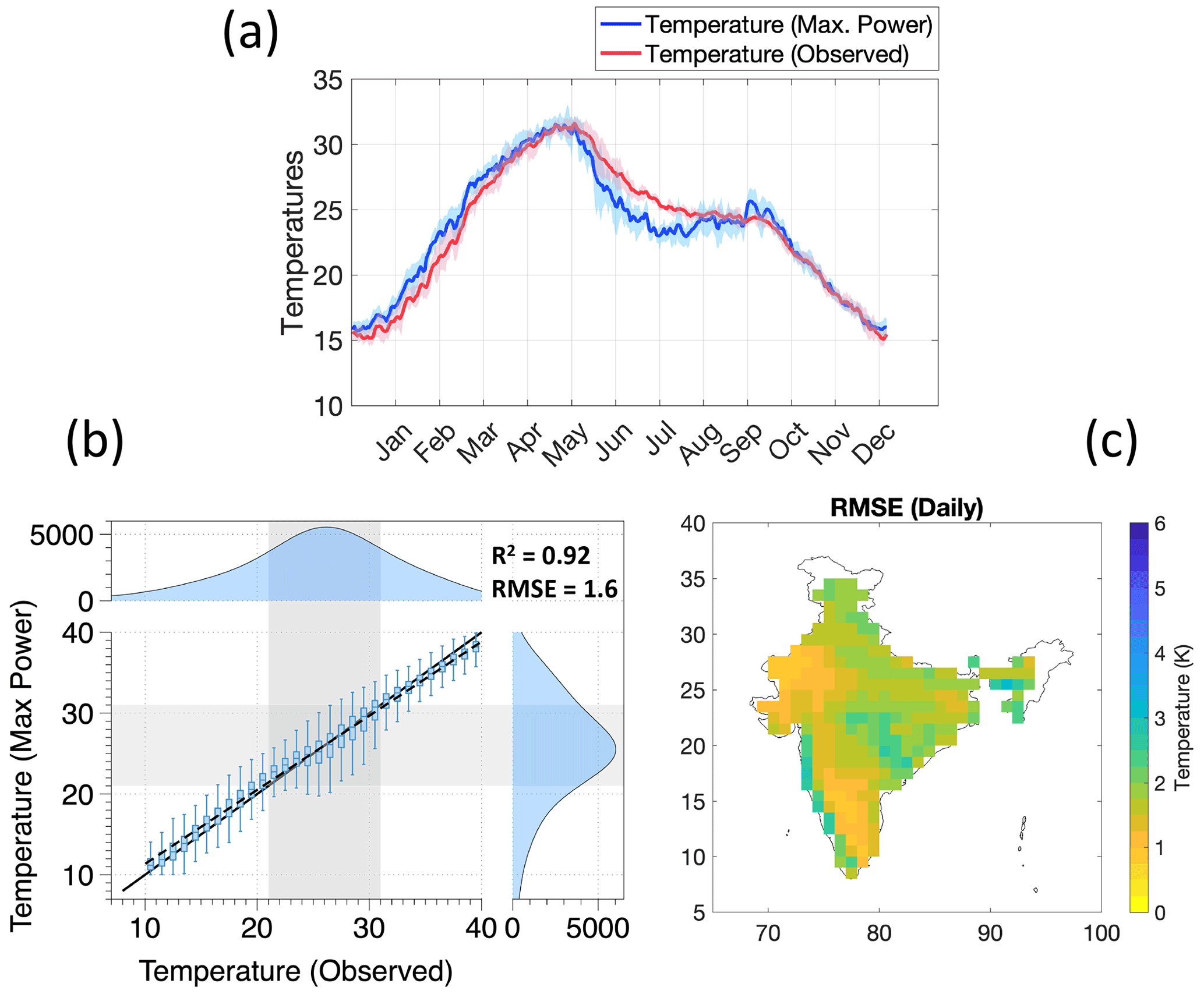
Figure 2(a) Comparison of daily annual cycle of temperature for observed (Indian Meteorological Department, IMD) and estimated all-sky surface temperatures, averaged over all grid points. (b) Regression between the two temperatures at the grid-point scale. (c) Spatial variation of the root mean squared error (RMSE) in temperature estimates from maximum power compared to observed temperatures.
3.2 Estimating the cloud radiative cooling
We used the difference between the all-sky and clear-sky temperatures as a measure to quantify the effect of cloud-driven cooling during rainfall events. This cooling strongly increases with precipitation across regions, resulting in a stronger reduction in surface temperature with greater precipitation (Fig. 3a); it is predominantly caused by the substantial reduction in absorbed solar radiation at the surface for all-sky conditions compared to clear-sky conditions (Fig. 3b). On the other hand, changes in long-wave radiation are comparatively small and remain largely insensitive to precipitation.
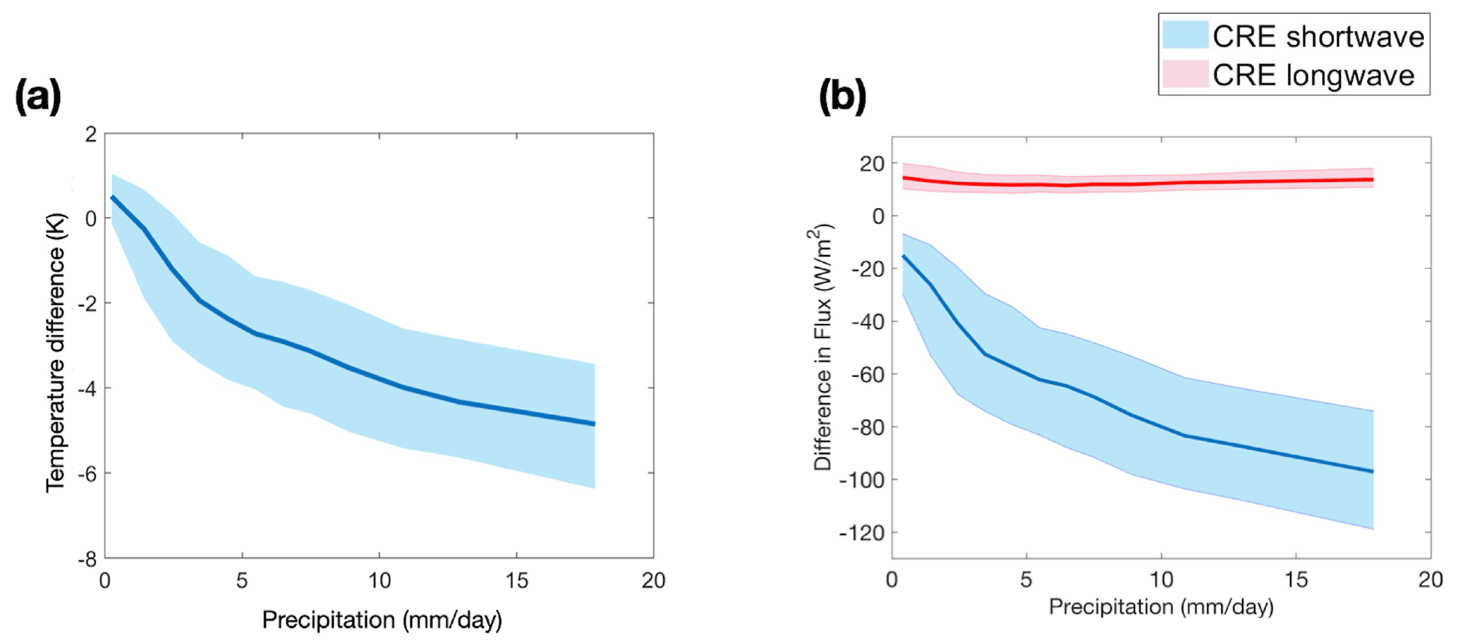
Figure 3(a) Cooling effect of clouds on surface temperatures calculated from the difference of all-sky to clear-sky surface temperatures as a function of precipitation over the Indian region. (b) Difference in net short-wave and downwelling long-wave radiative fluxes (cloud radiative effect, CRE) between all-sky and clear-sky radiative conditions at the surface as a function of precipitation. This was inferred using the NASA-CERES (EBAF ed4.1) dataset (Loeb et al., 2018).
To examine the spatial consistency in precipitation variability and associated cooling, we isolated extreme daily precipitation days over each grid. Figure 4a shows the mean magnitude of daily extreme precipitation events over India. The pattern was consistent with the cloud-cover map from NASA-CERES (shown in Appendix C). Figure 4b shows the cooling of clouds associated with these days. This cloud-cooling effect and precipitation shows a clear, systematic variation across India. The cooling effect is greater where precipitation rates are high. In contrast, in the more arid regions of northwestern India, the cooling effect almost disappears with low precipitation rates. In the northernmost Himalayan region, the difference in clear-sky and all-sky temperatures is negative. These high-altitude regions are more sensitive to changes in long-wave radiations. As a result, there is a significant increase in long-wave radiation with an increase in cloud cover that compensates for the cooling due to reduction in short wave over those grids. Figure 4c further shows the mean all-sky temperature during these days. We find that the heaviest events occur at a relatively lower temperature as a result of stronger cooling. Figure 4d shows the mean number of rainfall days per year. More rainy days implies more cloudy conditions and thus a stronger cloud radiative cooling over that region. Having quantified this effect of cloud radiative cooling and its systematic variation across regions, we then estimate its impact on the precipitation–temperature scaling.
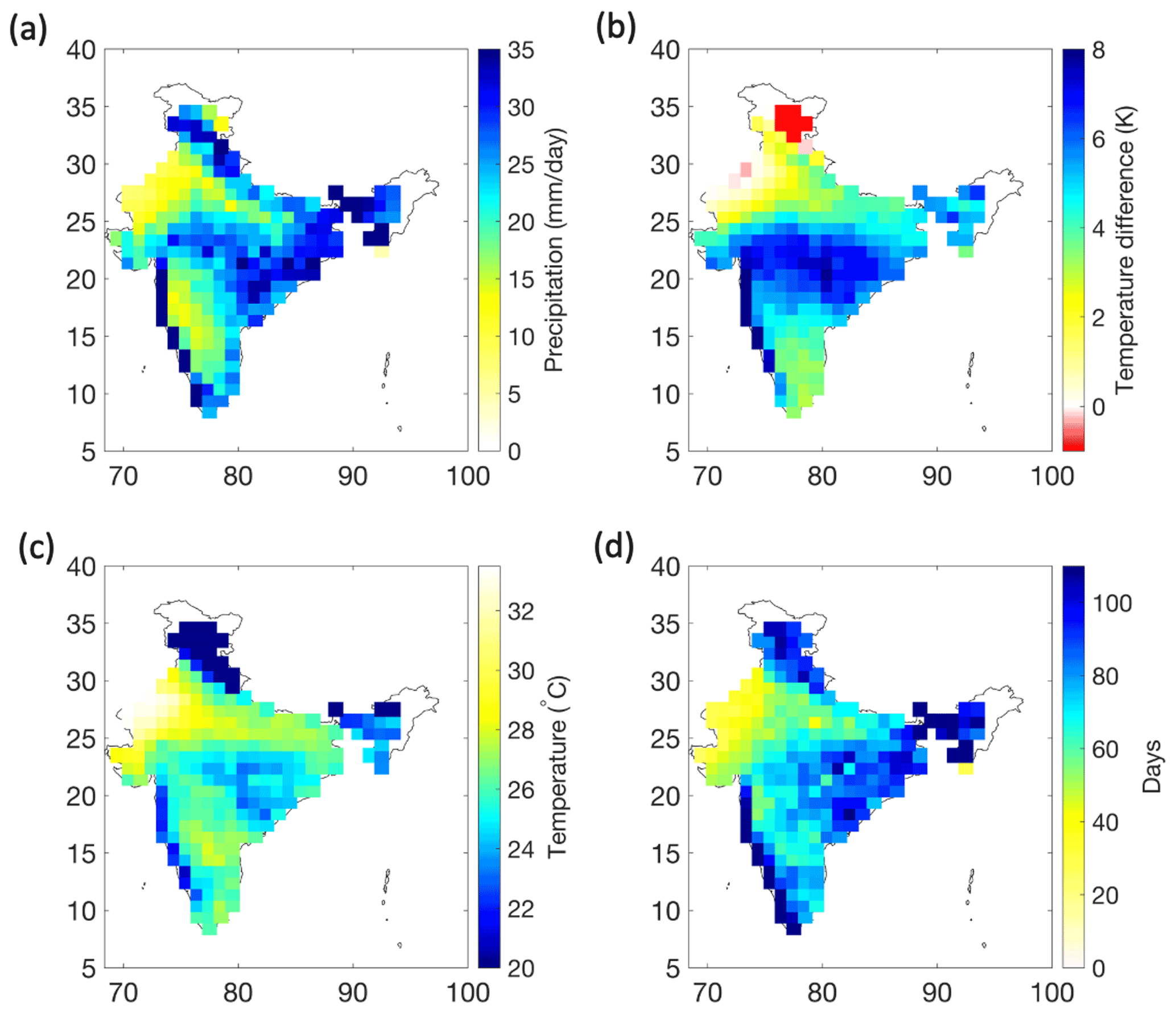
Figure 4Regional variation of (a) mean daily extreme precipitation (99th percentile), (b) the temperature difference between clear-sky and all-sky radiative conditions averaged during extreme precipitation events, (c) all-sky surface temperature during the occurrence of the event and (d) mean number of rainfall days per year.
3.3 Impact on precipitation-temperature scaling
We performed a binning analysis (Lenderink and Van Meijgaard, 2008) to understand the scaling of precipitation extremes with temperature using observed temperatures as well as our estimated clear-sky and all-sky temperatures. Precipitation events were isolated and binned into P–T pairs and the resulting scaling relationships are shown in Fig. 5. The scaling relationship using observed and all-sky temperatures showed similar scaling behaviour (yellow and red lines in Fig. 5a). Extreme precipitation increases close to the CC rate up to a threshold of around 23–24 ∘C, above which the scaling becomes negative. This breakdown in scaling behaviour with observed temperatures is consistent with the findings of previous studies (Hardwick Jones et al., 2010; Ghausi and Ghosh, 2020) and is commonly referred to in literature as “hook” or “peak structure” (Wang et al., 2017; Gao et al., 2018). However, when precipitation extremes are scaled with clear-sky temperatures that exclude the cloud-cooling effect, the resulting scaling relationship does not show a breakdown and increases consistently, close to the CC rate over the whole temperature range (blue line in Fig. 5a). Similar results were obtained when the scaling curves were reproduced for station-based observations (see Appendix A).

Figure 5(a) Extreme precipitation–temperature scaling using observed (yellow), all-sky (red) and clear-sky (blue) temperatures over India. (b) Same as (a), but using dew point temperatures. (c) Relationship between dew point temperatures and all-sky (red) and clear-sky (blue) temperatures. The shaded areas represent the variance in terms of the interquartile range for each bin. Dotted grey lines indicate the Clausius–Clapeyron (CC) scaling rate. Note the logarithmic vertical axis for panels (a) and (b).
Previous studies (Hardwick Jones et al., 2010; Chan et al., 2015; Wang et al., 2017) have attributed the breakdown in precipitation–temperature scaling to a lack of moisture availability as relative humidity tends to decrease at high temperatures. To account for this effect of moisture limitation, some studies used dew point temperature, a measure of atmospheric humidity, as an alternative scaling variable (Wasko et al., 2018; Barbero et al., 2018). They showed that the breakdown and negative scaling disappear when scaled with dew point temperatures (Zhang et al., 2019; Ali et al., 2021). To evaluate this interpretation and compare it to ours, we used the dew point temperature from the ERA-5 reanalysis. We derived the extreme precipitation scaling using this temperature (Fig. 5b) and compared it to our all-sky and clear-sky temperatures (Fig. 5c).
At first sight, the scaling relationship using dew point temperatures looks very similar to our clear-sky relationship (compare Fig. 5a and b, but note the difference in temperature scale). Yet, its interpretation differs because the use of dew point temperatures merely implies that the intensity of extreme precipitation events scales with the moisture content of the air, with moister air resulting in higher intensity events. Dew point scaling thus carries less insight about the response of extreme precipitation to global warming (Bao et al., 2018). To infer the precipitation sensitivity with temperature from dew point scaling, one then needs to see how dew point temperatures change with actual temperatures (dTdew dT) (Fig. 5c). This is further demonstrated using Eq. (10):
If relative humidity remains unchanged, we would expect the dew point temperature to increase continuously with surface temperature, representing a moisture increase of 7 % K−1. However, when dew point temperatures are compared to all-sky temperatures (red line, Fig. 5c), we note that a breakdown occurs in this scaling as well. Dew point temperatures increase with all-sky temperatures for colder temperatures more strongly than what would be expected from an unchanged relative humidity when air gets warmer. However, at temperatures above 23–25 ∘C, dew point temperatures fall, reflecting a decrease in relative humidity that is typical for warm, arid regions. Thus, one does not see a breakdown in precipitation–dew point scaling because the information on the breakdown is contained in how dew point temperatures change with surface air temperatures (second term in Eq. 10). Similar findings were also reported in Roderick et al. (2019).
The scaling of dew point temperatures with clear-sky temperatures is much more uniform and consistent across the whole temperature range; it does not show a breakdown or a super CC scaling in the relationship. This is because the clear-sky temperatures reflect the radiative conditions and not the effects of atmospheric humidity or clouds. In contrast, observed temperatures and all-sky temperatures covary with cloud effects, which in turn are linked to precipitation and humidity, thus resulting in less clear scaling relationships that are not as straightforward to interpret. This further implies that moisture loading of the atmosphere primarily occurs during the non-precipitating periods that are more representative of clear-sky radiative conditions.
The breakdown in scaling effect can thus be explained by the cooler temperatures associated with precipitation events. This cooling shifts the precipitation extremes to lower-temperature bins while the high-temperature bins correspond to more arid regions or to the drier pre-monsoon season temperatures with lower values of precipitation extremes. We refer to this as a “bin-shifting” effect. The cooling effect is proportional to the amount of precipitation (Fig. 3a) and hence, the heavier the precipitation, the stronger the cooling and bin shifting becomes. When the cloud-cooling effect is removed, as in the case of clear-sky temperatures, extreme precipitation then shows a scaling that is consistent with the CC rate. This bin-shifting effect arising due to the presence of clouds also causes a decrease in relative humidity at higher temperatures. This effect can be seen by the stronger increase in dew point temperatures below 25 ∘C and the decline above this temperature (Fig. 5c). The breakdown in scaling is thus not directly related to changes in aridity or moisture availability, but rather to the radiative effect of clouds on surface temperature.
To demonstrate the implications of our interpretation for precipitation scaling across regions, we estimated regression slopes of the 99th percentile precipitation events for both sub-daily (TRMM) and daily (IMD & APHRODITE) precipitation with the different temperatures using the quantile regression method (Wasko and Sharma, 2014). We found that extreme precipitation scaling was negative for both observed and all-sky temperatures over most regions (Fig. 6), except for the Himalayan foothills to the north of India. The scaling rates for sub-daily extremes were slightly higher than those estimated for daily extremes, yet they remain negative over most grids. When the cooling effect of clouds is removed by using clear-sky temperatures, extreme precipitation scaling then shows a diametric change and scaling estimates come close to CC rates over most of the regions. A similar diametric change in the scaling was also obtained with the APHRODITE precipitation dataset (Appendix B). The highest positive sensitivities were found over the region of central India where a widespread increase in rainfall extremes has already been reported (Roxy et al., 2017). There seems to be a minor difference between the clear-sky scaling in IMD and TRMM in the foothills of the Himalayas to the north of India, which is likely because of the underestimation of rainfall by TRMM over this region (Sharma et al., 2020; Shukla et al., 2019).
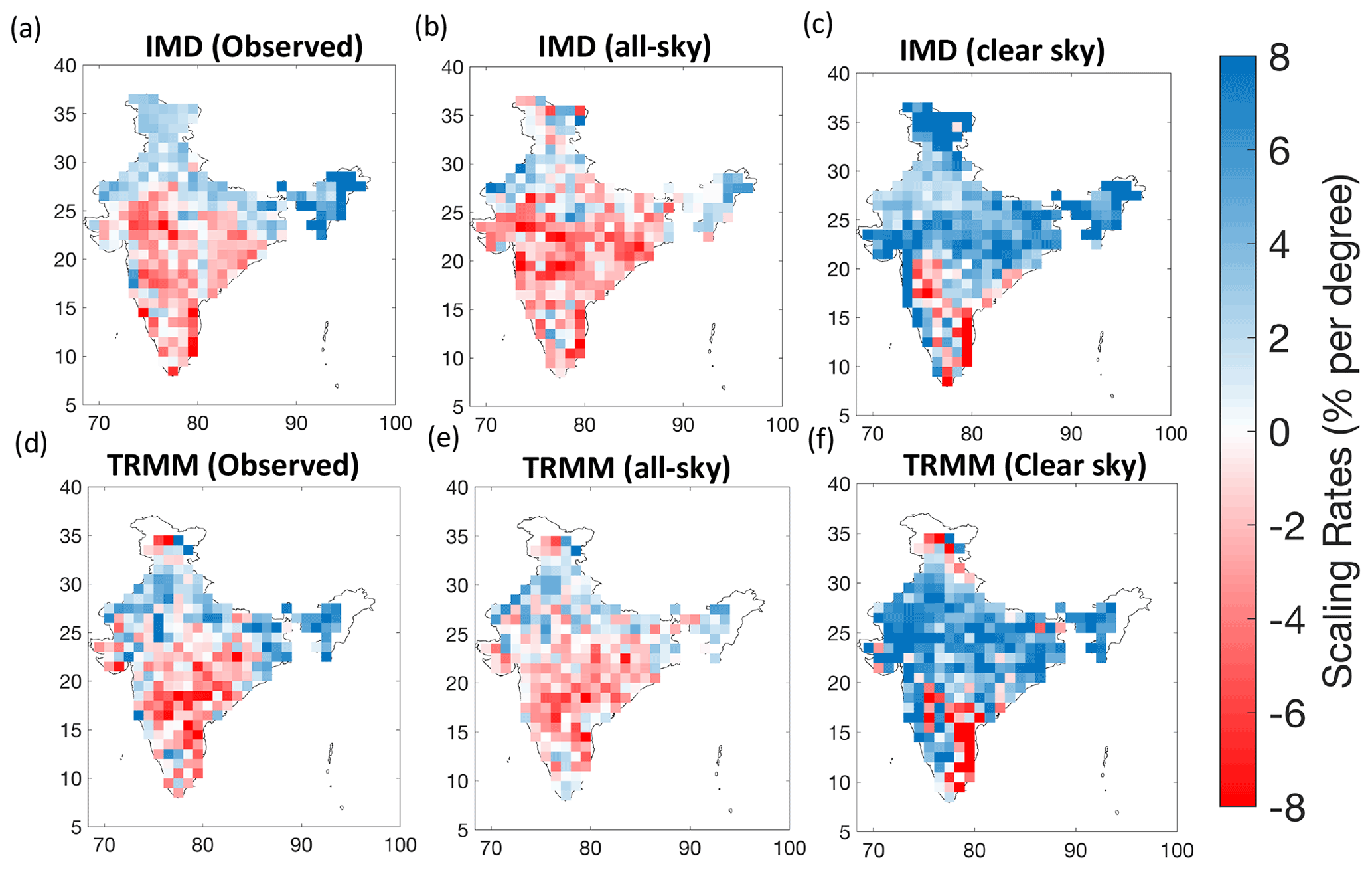
Figure 6Regional variation of the 99th percentile precipitation–temperature scaling rates using daily (a–c) and 3-hourly (d–f) rainfall data with observed temperatures (a, d), all-sky temperatures (b, e) and clear-sky temperatures (c, f).
We also note that negative scaling was found over a few regions of south-central and south-east India with clear-sky temperatures at both daily and sub-daily scales (Fig. 6c, f). To our understanding, this negative scaling primarily arises for two reasons. Firstly, these grids receive rainfall contributions during both the summer and winter monsoon, however, a relatively higher proportion of the rain occurs during the winter monsoon (Fig. C1). The is due to the fact that this region lies over the leeward side of the Western Ghats for the incoming south-west monsoon winds during the summer monsoon. Contrastingly, during the winter monsoon, north-east winds blow over the Bay of Bengal leading to large moisture advection and more rain over this region. As a result of this seasonality effect, more extreme precipitation is sampled during the winter season over this region while moisture supply may limit these extremes to increase during the summer season. This may lead to a negative scaling when a single quantile regression slope is fitted over the whole temperature range. Another reason could be the development of a low-pressure system in the Bay of Bengal during winter months which causes cyclones over the eastern coast of India. These cyclonic systems cause very high rainfall at very low temperatures which can lead to negative scaling (Traxl et al., 2021). It remains an important area for future research and more work is necessary to resolve these systems in conventional scaling approaches.
The effect of seasonality on precipitation scaling was also evaluated by producing the scaling curves for different seasonal subsets (summer and winter monsoon). We find a change in scaling during summer season after removing the cloud effects as the drop disappears (see Appendix C). The winter season, on the other hand, is associated with reduced rainfall amounts (less than 20 %) and less clouds over most regions resulting in a similar scaling for both all-sky and clear-sky temperatures.
While some differences exist, the cloud-cooling effect largely explains the negative scaling across most of the grid points over India. Extreme precipitation increases monotonically with temperature when the cloud-cooling effect is removed. This implies that the peak structures obtained with observed scaling will not constrain the rise in extremes with anthropogenic warming. Moreover, the confounding effect between precipitation and temperature on observed scaling relationships, also termed “apparent scaling”, had been argued by some recent studies (Bao et al. 2017; Visser et al., 2020). Our results agree with these studies in that the observed scaling relationships also reflect the impact of synoptic conditions and cooling associated with precipitation events on temperature. However, we suggest that this confounding effect is largely associated with cloud radiative effect, which is removed by our use of clear-sky temperatures as a scaling variable. Additionally, we address the arguments raised to resolve apparent scaling using dew point temperature (Barbero et al., 2018). Our results confirm that precipitation extremes scale well with dew point temperatures as a measure for atmospheric moisture, but that the breakdown in scaling actually originates from the scaling of dew point temperatures with observed temperatures. This response of dew point temperature to warming is further affected by the presence of clouds and associated radiative cooling. Clear-sky temperatures are independent of the covariations arising from cloud effects and are thus a better, more independent measure and scaling variable for understanding the precipitation response to global warming.
We showed that the observed negative scaling of extreme precipitation in India arises mostly from the cloud radiative cooling of surface temperatures. When this effect is removed, we get a positive scaling consistent with the CC rate. Scaling rates estimated from observed temperatures are thus likely to misrepresent the response of extreme precipitation to global warming, because the cooling effects of clouds make precipitation and temperature covary with each other. When this effect is removed by estimating surface temperatures for clear-sky conditions, the scaling relationships with moisture content and precipitation become much clearer and confirm the CC scaling of extreme precipitation events with warmer temperatures. This explains the apparent discrepancy between the observed negative scaling rates over India and the projected increase in precipitation extremes by climate models.
While scaling with clear-sky temperatures shows a diametric change and significant improvement over observed scaling, regional variabilities in scaling rates and deviations from CC scaling (7 % K−1) still exist. We believe that these deviations could be due to the following reasons: firstly, the present scaling approach does not explicitly consider the contribution from the large-scale dynamics and regional circulation patterns which can cause local changes in the scaling estimates. Secondly, the effect of change in rainfall types – orographic, stratiform or convective – is not accounted for and it can affect the estimates of scaling rates. Lastly, inconsistencies between precipitation and radiation datasets can cause uncertainties in estimating the cooling associated with rainfall events and can affect the estimates of scaling rates.
It is also important to note that the goal of our study was not to compare the accuracy of scaling estimates from different gridded and station-based datasets, but rather to identify and remove the physical effects that cause uncertainties in this response. Our methodology to remove the cooling effect of clouds from surface temperatures significantly improves the scaling estimate for daily precipitation scaling.
While our study was confined to the Indian region, we would expect that cloud effects on surface temperatures can explain the deviations in precipitation scaling from CC rates in other tropical regions as well. Furthermore, our methodology to remove the cloud-cooling effects on surface temperatures could also be extended to derive scaling relationships of other, observed variables to obtain their response to global warming. Our findings add a novel component to better interpret precipitation scaling rates derived from observations to support climate model projections.
We used three station-based daily observations from GSOD data provided by NOAA. We used the data from the airports in Mumbai, Chennai and Bangalore to produce the scaling curves (Appendix A). Since the three sites receive rainfall during different periods of the year, the choice of station was based on ensuring the robustness of results using gauge data as well as checking the effect of seasonality. In Mumbai, rainfall occurs mainly during the summer monsoon season while in Chennai heavy rainfall occurs during the winter months (November and December). On other hand, Bangalore receives rainfall during both the summer and winter monsoon season (Fig. A1 – row 1). Negative scaling was found over these three stations using observed (yellow) and all-sky (red) temperatures while with clear-sky temperatures (blue), we find positive rates largely consistent with the CC rate.
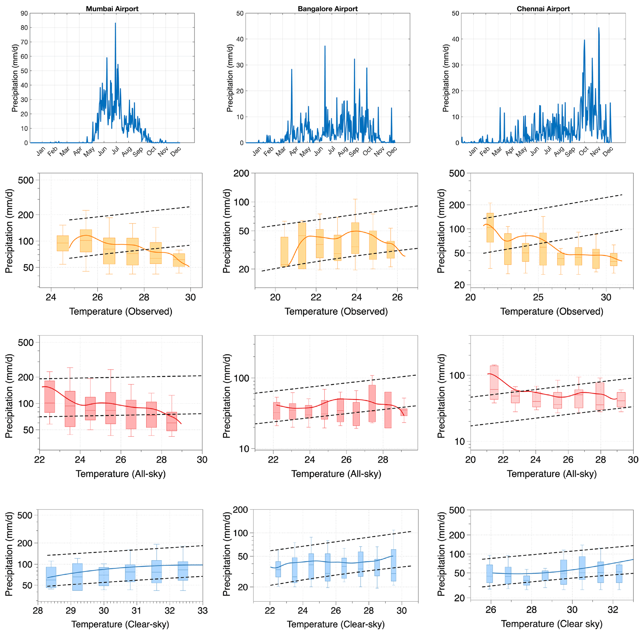
Figure A1Row 1 shows the annual cycle of mean daily precipitation over GSOD sites in Mumbai airport, Bangalore airport and Chennai airport, respectively. Extreme precipitation–temperature scaling curves for observed temperatures (yellow), all-sky temperatures (red) and clear-sky temperatures (in blue) are presented for all the three sites. Solid yellow/red/blue lines indicate the LOESS regression lines. Dotted grey lines indicate the Clausius–Clapeyron (CC) scaling rate. Note the logarithmic vertical axis.
Figure B1 shows the spatial variation of daily precipitation–temperature scaling rates estimated from quantile regression (similar to Fig. 6 in the main text) using the Asian Precipitation Highly-Resolved Observational Data Integration towards Evaluation of water resources (APHRODITE) dataset (Yatagai et al., 2012). The results show a diametric change in scaling from being negative for observed and all-sky temperatures to coming close to the CC rate (7 % K−1) for clear-sky temperatures. The findings were consistent with that obtained using the IMD and TRMM datasets (Fig. 6).
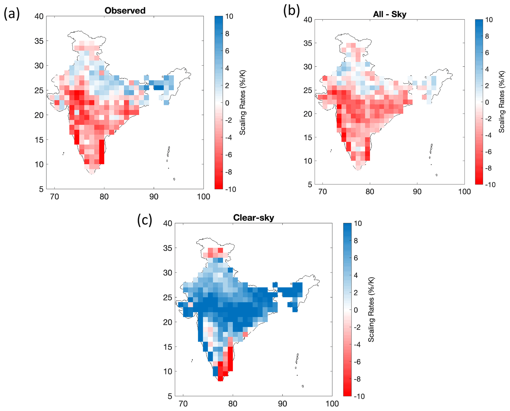
Figure B1Regional variation of the 99th percentile daily precipitation–temperature scaling rates using (a) observed (b) all-sky and (c) clear-sky temperatures. Note that precipitation data are from the APHRODITE dataset.
To understand the role of seasonality on precipitation–temperature scaling. We divided the precipitation period into two seasonal subsets, i.e. summer monsoon season (April to September) and winter monsoon (October to March). Season-wise scaling curves (estimated using the LOESS regression) are presented in Fig. C3. We find that observed scaling is uniformly negative during summer over the Indian region while the scaling is positive during winter (Fig. C3a, d). This is not surprising because the “hook” or breakdown in scaling happens at high temperatures which leads to negative scaling in summer (Fig. 5a). Reconstructed all-sky temperature showed scaling patterns consistent with observations (Fig. C3b, e). When scaled with clear-sky temperatures, we observed a change in scaling for summer as it turns positive and comes close to the CC rate, while the scaling does not change for clear-sky temperatures during winter. It is also important to note that almost 80 % of the total rainfall over India occurs during the summer monsoon season (Fig. C1). As a result, the cooling effect of clouds is mainly experienced during the summer monsoon (where we observed a change in scaling) while the cooling effect remains less than 1 K during the winter season (Fig. C2). Thus, one does not see a change in scaling between all-sky and clear-sky conditions for the winter season.
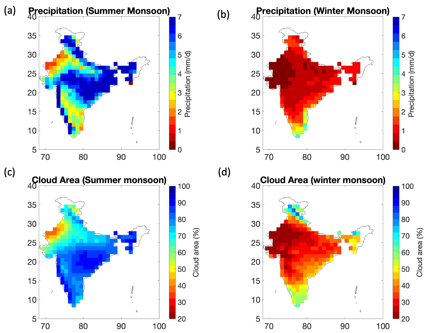
Figure C1Maps of the mean daily precipitation (from IMD) and cloud area fraction (from NASA-CERES) during (a, c) the summer monsoon (April–September) and during (b, d) the winter monsoon (October–March).
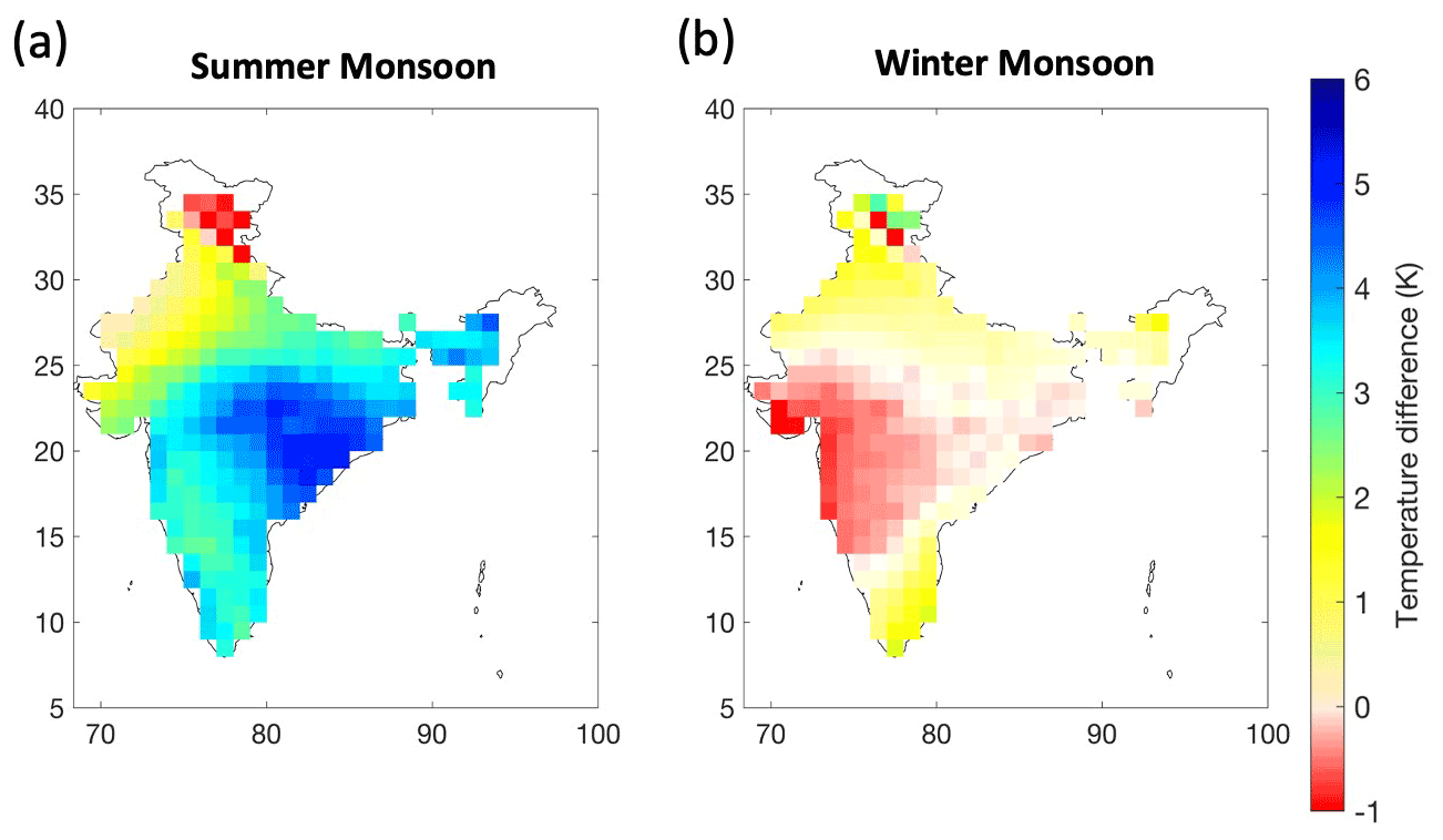
Figure C2Maps of the cooling of surface due to clouds (defined as the difference between clear-sky and all-sky temperatures) for the (a) summer monsoon (April–September) and (b) winter monsoon (October–March).
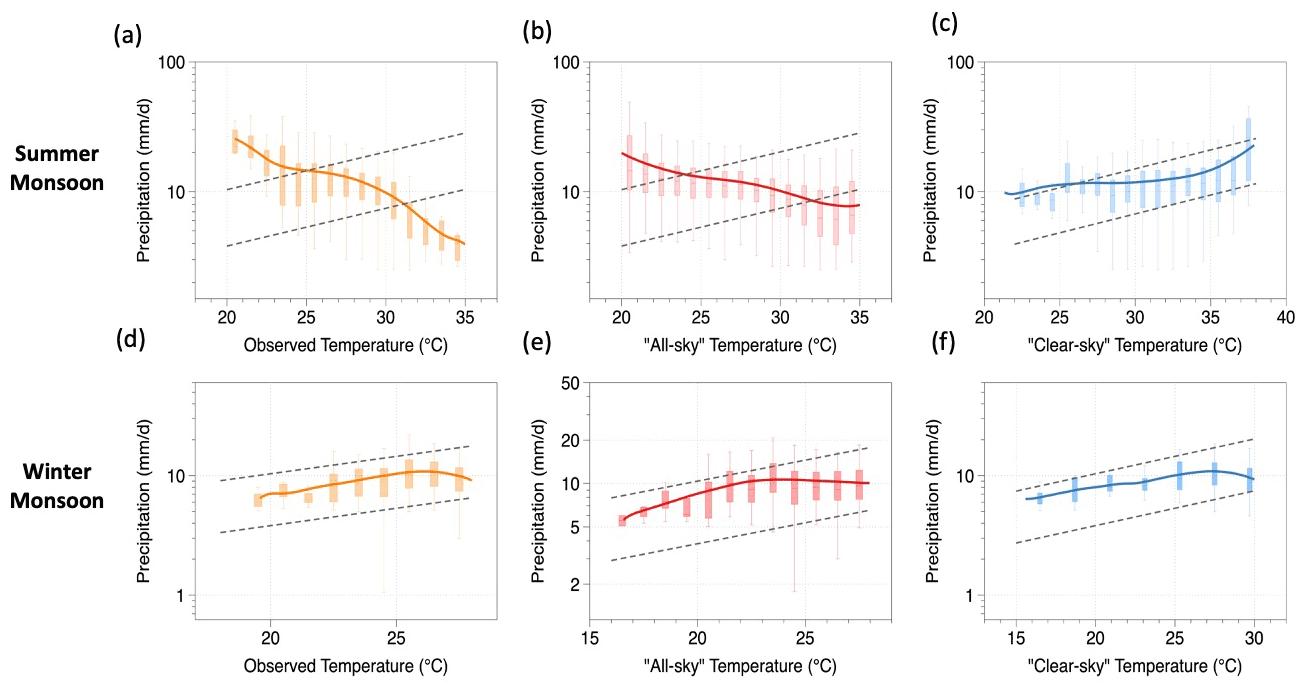
Figure C3Extreme precipitation–temperature scaling during the summer monsoon (a–c) and winter monsoon (d–f). Scaling curves are shown in yellow for observed temperatures (a, d), in red for all-sky temperatures (b, e) and in blue for clear-sky temperatures (c, f). Solid yellow/red/blue lines indicate the LOESS regression lines. Dotted grey lines indicate the Clausius–Clapeyron (CC) scaling rate. Note the logarithmic vertical axis. Dataset used is IMD.
The daily gridded precipitation and temperature datasets were obtained from the India Meteorological Department (https://www.imdpune.gov.in/Clim_Pred_LRF_New/Grided_Data_Download.html, Climate Monitoring and Prediction Group, Indian Meteorological Department, 2020). The APHRODITE (Asian Precipitation Highly-Resolved Observational Data Integration towards Evaluation) dataset is available at http://aphrodite.st.hirosaki-u.ac.jp/download/ (Yatagai et al., 2020). Sub-daily precipitation data at 3-hourly resolution were obtained from TRMM (Tropical Rainfall measuring mission) TMPA_3B42_V7 data (https://doi.org/10.5067/TRMM/TMPA/3H/7, TRMM, 2011). Station-based daily precipitation–temperature data were taken from NOAA-GSOD sites (station ID: 43295099999, 43003099999 and 43279099999) at https://www.ncei.noaa.gov/access/search/data-search/global-summary-of-the-day (NCEI and NOAA, 2020). Surface and TOA gridded radiative flux datasets are obtained from NASA-CERES EBAF data (https://doi.org/10.5067/Terra-Aqua/CERES/EBAF_L3B.004.1, NASA Langley Research Center, Atmospheric Science Data Center, 2020) and NASA-CERES Syn1deg data (https://doi.org/10.5067/Terra+Aqua/CERES/SYN1degDay_L3. 004A, NASA Langley Research Center, Atmospheric Science Data Center, 2021). Daily dew point temperature data are obtained from the ERA-5 reanalysis (https://doi.org/10.24381/cds.e2161bac, Muñoz Sabater, 2019).
All the authors contributed to the idea and development of the hypothesis. SAG carried out the data analysis. The writing of the manuscript was done by SAG with inputs and edits from AK. AK and SAG helped to design the study. All the authors contributed to the interpretation of the results.
The contact author has declared that none of the authors has any competing interests.
Publisher’s note: Copernicus Publications remains neutral with regard to jurisdictional claims in published maps and institutional affiliations.
We would like to thank the three anonymous reviewers and the editor for their comments. The author thanks the NASA-CERES team for making the satellite data openly available, the Copernicus Climate Change Service for access to the ERA-5 reanalysis data, India Meteorological Department (IMD) for access to rainfall data and the APHRODITE group for providing free access to their rainfall dataset.
This research has been supported by the Max-Planck-Gesellschaft (IMPRS for global biogeochemical cycles).
The article processing charges for this open-access publication were covered by the Max Planck Society.
This paper was edited by Xing Yuan and reviewed by three anonymous referees.
Ali, H., Fowler, H. J., Lenderink, G., Lewis, E., and Pritchard, D. Consistent large-scale response of hourly extreme precipitation to temperature variation over land, Geophys. Res. Lett., 48, e2020GL090317, https://doi.org/10.1029/2020GL090317, 2021.
Allen, M. and Ingram, W.: Constraints on future changes in climate and the hydrologic cycle, Nature, 419, 228–232, https://doi.org/10.1038/nature01092, 2002.
Ban, N.,Schmidli, J., and Schär, C.: Heavy precipitation in a changing climate: Does short-term summer precipitation increase faster?, Geophys. Res. Lett., 42, 1165–1172, https://doi.org/10.1002/2014GL062588, 2015.
Bao, J., Sherwood, S. C., Alexander, L. V., and Evans, J. P.: Future increases in extreme precipitation exceed observed scaling rates, Nat. Clim. Change, 7, 128–132, https://doi.org/10.1038/nclimate3201, 2017.
Bao, J., Sherwood, S. C., Alexander, L. V., and Evans, J. P.: Comments on “temperature-extreme precipitation scaling: A two-way causality?”, Int. J. Climatol., 38, 4661–4663, 2018.
Barbero, R., Westra, S., Lenderink, G., and Fowler, H. J.: Temperature-extreme precipitation scaling: a two-way causality?, Int. J. Climatol., 38, e1274–e1279, 2018.
Berg, P., Moseley, C., and Haerter, J. O.: Strong increase in convective precipitation in response to higher temperatures, Nat. Geosci., 6, 181–185, https://doi.org/10.1038/ngeo1731, 2013.
Bui, A., Johnson, F., and Wasko, C.: The relationship of atmospheric air temperature and dew point temperature to extreme rainfall, Environ. Res. Lett., 14, 074025, https://doi.org/10.1088/1748-9326/ab2a26, 2019.
Chan, S. C., Kendon, E. J., Roberts, N. M., Fowler, H. J., and Blenkinsop, S.: Downturn in scaling of UK extreme rainfall with temperature for future hottest days, Nat. Geosci., 9, 24–28, https://doi.org/10.1038/ngeo2596, 2015.
Climate Monitoring and Prediction Group, Indian Meteorological Department: IMD Gridded Rainfall dataset, [data set], https://www.imdpune.gov.in/Clim_Pred_LRF_New/Grided_Data_Download.html, last access: 20 August 2020.
Dhara, C., Renner, M., and Kleidon, A.: Broad climatological variation of surface energy balance partitioning across land and ocean predicted from the maximum power limit, Geophys. Res. Lett., 43, 7686–7693, https://doi.org/10.1002/2016GL070323, 2016.
Doelling, D. R., Loeb, N. G., Keyes, D. F., Nordeen, M. L., Morstad, D., Nguyen, C., and Sun, M.: Geostationary enhanced temporal interpolation for CERES flux products, J. Atmos. Ocean. Tech., 30, 1072–1090, 2013.
Doelling, D. R., Sun, M., Nguyen, L. T., Nordeen, M. L., Haney, C. O., Keyes, D. F., and Mlynczak, P. E.: Advances in geostationary-derived longwave fluxes for the CERES synoptic (SYN1 deg) product, J. Atmos. Ocean. Tech., 33, 503–521, 2016.
Donat, M. G., Lowry, A. L., Alexander, L. V., O'Gorman, P. A., and Maher, N. More extreme precipitation in the world's dry and wet regions, Nat. Clim. Change, 6, 508–513, 2016.
Fischer, E. M., Beyerle, U., and Knutti, R.: Robust spatially aggregated projections of climate extremes, Nat. Clim. Change, 3, 1033–1038, 2013.
Gao, X., Zhu, Q., Yang, Z., Liu, J., Wang, H., Shao, W., and Huang, G.: Temperature Dependence of Hourly, Daily, and Event-based Precipitation Extremes Over China, Sci. Rep.-UK, 8, 1–10, https://doi.org/10.1038/s41598-018-35405-4, 2018.
Ghausi, S. A. and Ghosh, S.: Diametrically Opposite Scaling of Extreme Precipitation and Stream flow to Temperature in South and Central Asia, 47, e2020GL089386, https://doi.org/10.1029/2020GL089386, 2020.
Golroudbary, V. R., Zeng, Y., Mannaerts, C. M., and Su, Z.: Response of extreme precipitation to urbanization over the Netherlands, J. Appl. Meteorol. Clim., 58, 645–661, https://doi.org/10.1175/jamc-d-18-0180.1, 2019.
Goswami, B. N., Venugopal, V., Sengupta, D., Madhusoodanan, M. S., and Xavier, P. K.: Increasing trend of extreme rain events over India in a warming environment, Science, 314, 1442–1445, https://doi.org/10.1126/science.1132027, 2006.
Hardwick Jones, R., Westra, S., and Sharma, A.: Observed relationships between extreme sub-daily precipitation, surface temperature, and relative humidity, Geophys. Res. Lett., 37, L22805, https://doi.org/10.1029/2010GL045081, 2010.
Held, I. M. and Soden, B. J.: Robust responses of the hydrological cycle to global warming, J. Climate, 19, 5686–5699, 2006.
Kato, S., Rose, F. G., Rutan, D. A., Thorsen, T. E., Loeb, N. G., Doelling, D. R., Huang, X., Smith, W. L., Su, W., and Ham, S.-H.: Surface irradiances of Edition 4.0 Clouds and the Earth's Radiant Energy System (CERES) Energy Balanced and Filled (EBAF) data product, J. Climate, 31, 4501–4527, https://doi.org/10.1175/JCLI-D-17-0523.1, 2018.
Katzenberger, A., Schewe, J., Pongratz, J., and Levermann, A.: Robust increase of Indian monsoon rainfall and its variability under future warming in CMIP6 models, Earth Syst. Dynam., 12, 367–386, https://doi.org/10.5194/esd-12-367-2021, 2021.
Kendon, E. J., Roberts, N. M., Fowler, H. J., Roberts, M. J., Chan, S. C., and Senior, C. A.: Heavier summer downpours with climate change revealed by weather forecast resolution model, Nat. Clim. Change, 4, 570–576, https://doi.org/10.1038/nclimate2258, 2014.
Kleidon, A. and Renner, M.: A simple explanation for the sensitivity of the hydrologic cycle to surface temperature and solar radiation and its implications for global climate change, Earth Syst. Dynam., 4, 455–465, https://doi.org/10.5194/esd-4-455-2013, 2013.
Kleidon, A., Renner, M., and Porada, P.: Estimates of the climatological land surface energy and water balance derived from maximum convective power, Hydrol. Earth Syst. Sci., 18, 2201–2218, https://doi.org/10.5194/hess-18-2201-2014, 2014.
Lenderink, G. and Van Meijgaard, E.: Increase in hourly precipitation extremes beyond expectations from temperature changes, Nat. Geosci., 1, 511–514, https://doi.org/10.1038/ngeo262, 2008.
Lenderink, G. and Van Meijgaard, E.: Linking increases in hourly precipitation extremes to atmospheric temperature and moisture changes, Environ. Res. Lett., 5, 025208, https://doi.org/10.1088/1748-9326/5/2/025208, 2010.
Loeb, N. G., Doelling, D. R., Wang, H., Su, W., Nguyen, C., Corbett, J. G., Liang, L., Mitrescu, C., Rose, F. G., and Kato, S.: Clouds and the Earth's Radiant Energy System (CERES) Energy Balanced and Filled (EBAF) Top-of-Atmosphere (TOA) Edition-4.0 data product, J. Climate, 31, 895–918, https://doi.org/10.1175/JCLI-D-17-0208.1, 2018.
Molnar, P., Fatichi, S., Gaál, L., Szolgay, J., and Burlando, P.: Storm type effects on super Clausius–Clapeyron scaling of intense rainstorm properties with air temperature, Hydrol. Earth Syst. Sci., 19, 1753–1766, https://doi.org/10.5194/hess-19-1753-2015, 2015.
Mukherjee, S., Saran, A., Stone, D., and Mishra, V.: Increase in extreme precipitation events under anthropogenic warming in India, Weather Clim. Extrem., 20, 45–53, https://doi.org/10.1016/j.wace.2018.03.005, 2018.
Muñoz Sabater, J.: ERA5-Land hourly data from 1981 to present, Copernicus Climate Change Service (C3S) Climate Data Store (CDS) [data set], https://doi.org/10.24381/cds.e2161bac, 2019.
National Centers for Environmental Information (NCEI), National Oceanic and Atmospheric Administration (NOAA): GSOD Rainfall data, https://www.ncei.noaa.gov/access/search/data-search/global-summary-of-the-day, last access: 15 October 2021.
NASA Langley Research Center, Atmospheric Science Data Center: CERES_EBAF_Edition4.1, https://doi.org/10.5067/TERRA-AQUA/CERES/EBAF_L3B.004.1, 2020.
NASA Langley Research Center, Atmospheric Science Data Center: CER_SYN1deg-Day_Terra-Aqua-MODIS_Edition4A, [data set], https://doi.org/10.5067/Terra+Aqua/CERES/SYN1degDay_L3.004A, 2021.
O'Gorman, P. A. and Schneider, T.: The physical basis for increases in precipitation extremes in simulations of 21st-century climate change, P. Natl. Acad. Sci. USA, 106, 14773–14777, 2009.
Rajeevan, M., Jyoti Bhate, and Jaswal, A. K.: Analysis of variability and trends of extreme rainfall events over India using 104 years of gridded daily rainfall data, Geophys. Res. Lett., 35, L18707, https://doi.org/10.1029/2008GL035143, 2008.
Roderick, T. P., Wasko, C., and Sharma, A.: Atmospheric moisture measurements explain increases in tropical rainfall extremes, Geophys. Res. Lett., 46, 1375–1382, https://doi.org/10.1029/2018GL080833, 2019.
Roxy, M. K., Ghosh, S., Pathak, A., Athulya, R., Mujumdar, M., Murtugudde, R., Terray P., and Rajeevan, M.: A threefold rise in widespread extreme rain events over central India, Nat. Commun., 8, 1–11, https://doi.org/10.1038/s41467-017-00744-9, 2017.
Schroeer, K. and Kirchengast, G.: Sensitivity of extreme precipitation to temperature: the variability of scaling factors from a regional to local perspective, Clim. Dynam., 50, 3981–3994, https://doi.org/10.1007/s00382-017-3857-9, 2018.
Sharma, S. and Mujumdar, P. P.: On the relationship of daily rainfall extremes and local mean temperature, J. Hydrol., 572, 179–191, https://doi.org/10.1016/j.jhydrol.2019.02.048, 2019.
Sharma, S., Khadka, N., Hamal, K., Shrestha, D., Talchabhadel, R., and Chen, Y.: How accurately can satellite products (TMPA and IMERG) detect precipitation patterns, extremities, and drought across the Nepalese Himalaya?, Earth and Space Science, 7, e2020EA001315, https://doi.org/10.1029/2020EA001315, 2020.
Shukla, A. K., Ojha, C. S. P., Singh, R. P., Pal, L., and Fu, D.: Evaluation of TRMM Precipitation Dataset over Himalayan Catchment: The Upper Ganga Basin, India, Water, 11, 613, https://doi.org/10.3390/w11030613, 2019.
Sun, Q., Zwiers, F., Zhang, X., and Li, G.: A comparison of intra-annual and long-term trend scaling of extreme precipitation with temperature in a large-ensemble regional climate simulation, J. Climate, 33, 9233–9245, 2020.
Traxl, D., Boers, N., Rheinwalt, A., and Bookhagen B.: The role of cyclonic activity in tropical temperature-rainfall scaling, Nat. Commun., 12, 6732, https://doi.org/10.1038/s41467-021-27111-z, 2021.
Trenberth, K. E., Dai, A., Rasmussen, R. M., and Parsons, D. B.: The changing character of precipitation, B. Am. Meteorol. Soc., 84, 1205–1217, https://doi.org/10.1175/BAMS-84-9-1205, 2003.
Tropical Rainfall Measuring Mission (TRMM): TRMM (TMPA) Rainfall Estimate L3 3-hour 0.25-degree × 0.25-degree V7, Greenbelt, MD, Goddard Earth Sciences Data and Information Services Center (GES DISC) [data set], https://doi.org/10.5067/TRMM/TMPA/3H/7, 2011.
Utsumi, N., Seto, S., Kanae, S., Maeda, E. E., and Oki, T.: Does higher surface temperature intensify extreme precipitation?, Geophys. Res. Lett., 38, L16708, https://doi.org/10.1029/2011GL048426, 2011.
Visser, J. B., Wasko, C., Sharma, A., and Nathan, R.: Resolving Inconsistencies in Extreme Precipitation-Temperature Sensitivities, Geophys. Res. Lett., 47, e2020GL089723, https://doi.org/10.1029/2020GL089723, 2020.
Visser, J. B., Wasko, C., Sharma, A., and Nathan, R.: Eliminating the “Hook” in Precipitation–Temperature Scaling, J. Climate, 34, 9535–9549, https://doi.org/10.1175/JCLI-D-21-0292.1, 2021.
Vittal, H., Ghosh, S., Karmakar, S., Pathak, A., and Murtugudde, R.: Lack of Dependence of Indian Summer Monsoon Rainfall Extremes on Temperature: An Observational Evidence, Sci. Rep.-UK, 6, 31039, https://doi.org/10.1038/srep31039, 2016.
Wang, G., Wang, D., Trenberth, K. E., Erfanian, A., Yu, M., Bosilovich, M. G., and Parr, D. T.: The peak structure and future changes of the relationships between extreme precipitation and temperature, Nat. Clim. Change, 7, 268–274, https://doi.org/10.1038/nclimate3239, 2017.
Wasko, C. and Sharma, A.: Quantile regression for investigating scaling of extreme precipitation with temperature, Water Resour. Res., 50, 3608–3614, https://doi.org/10.1002/2013WR015194, 2014.
Wasko, C., Lu, W. T., and Mehrotra, R.: Relationship of extreme precipitation, dry-bulb temperature, and dew point temperature across Australia, Environ. Res. Lett., 13, 074031, https://doi.org/10.1088/1748-9326/aad135, 2018.
Westra, S., Alexander, L. V., and Zwiers, F. W.: Global increasing trends in annual maximum daily precipitation, J. Climate, 26, 3904–3918, https://doi.org/10.1175/JCLI-D-12-00502.1, 2013.
Westra, S., Fowler, H. J., Evans, J. P., Alexander, L. V., Berg, P., Jonson, F., Kendon, E. J., Lenderink, G., and Roberts, N. M.: Future changes to the intensity and frequency of short-duration extreme rainfall, Rev. Geophys., 52, 522–555, https://doi.org/10.1002/2014RG000464, 2014.
Yatagai, A., Kamiguchi, K., Arakawa, O., Hamada, A., Yasutomi, N., and Kitoh, A.: Aphrodite constructing a long-term daily gridded precipitation dataset for Asia based on a dense network of rain gauges, B. Am. Meteorol. Soc., 93, 1401–1415, https://doi.org/10.1175/BAMS-D-11-00122.1, 2012.
Yatagai, A., Kamiguchi, K., Arakawa, O., Hamada, A., Yasutomi, N., and Kitoh, A.: APHRODITE daily rainfall data (V_1901), http://aphrodite.st.hirosaki-u.ac.jp/download/, last access: 20 August 2020.
Zhang, W., Villarini, G., and Wehner, M.: Contrasting the responses of extreme precipitation to changes in surface air and dew point temperatures, Climatic Change, 154, 257–271, https://doi.org/10.1007/s10584-019-02415-8, 2019.
- Abstract
- Introduction
- Methods and data
- Results and discussion
- Summary and conclusions
- Appendix A: Validation of scaling results using station-based GSOD data
- Appendix B: Validation of scaling results using APHRODITE dataset
- Appendix C: Effect of seasonality on scaling rates
- Data availability
- Author contributions
- Competing interests
- Disclaimer
- Acknowledgements
- Financial support
- Review statement
- References