Quantifying overlapping and differing information of global precipitation for GCM forecasts and El Niño–Southern Oscillation

While El Niño–Southern Oscillation (ENSO) teleconnection has long been used in statistical precipitation forecasting, global climate models (GCMs) provide increasingly available dynamical precipitation forecasts for hydrological modeling and water resources management. It is not yet known to what extent dynamical GCM forecasts provide new information compared to statistical teleconnection. This paper develops a novel set operations of coefficients of determination (SOCD) method to explicitly quantify the overlapping and differing information for GCM forecasts and ENSO teleconnection. Specifically, the intersection operation of the coefficient of determination derives the overlapping information for GCM forecasts and the Niño3.4 index, and then the difference operation determines the differing information in GCM forecasts (Niño3.4 index) from the Niño3.4 index (GCM forecasts). A case study is devised for the Climate Forecast System version 2 (CFSv2) seasonal forecasts of global precipitation in December–January–February. The results show that the overlapping information for GCM forecasts and the Niño3.4 index is significant for 34.94 % of the global land grid cells, that the differing information in GCM forecasts from the Niño3.4 index is significant for 31.18 % of the grid cells and that the differing information in the Niño3.4 index from GCM forecasts is significant for 11.37 % of the grid cells. These results confirm the effectiveness of GCMs in capturing the ENSO-related variability of global precipitation and illustrate where there is room for improvement of GCM forecasts. Furthermore, the bootstrapping significance tests of the three types of information facilitate in total eight patterns to disentangle the close but divergent associations of GCM forecast correlation skill with ENSO teleconnection.

1 Introduction

Seasonal precipitation forecasts are important for agricultural scheduling, water management and drought mitigation (Sheffield et al., 2014; Anghileri et al., 2016; Peng et al., 2018; He et al., 2019; Zhao et al., 2019). Performing hydrological forecasting into the future, the uncertainty generally arises from catchment initial conditions and future climate forcings (Wood and Lettenmaier, 2006; Yuan et al., 2014; Huang et al., 2020). In a short lead time up to about 1 month, initial conditions tend to outweigh climate forcings; at longer lead times, climate forcings become a more important contributor (Li et al., 2009; Yossef et al., 2013). Therefore, besides remote sensing-based estimations of initial conditions of snow cover, soil moisture and groundwater storage (Mei et al., 2020; W. Xu et al., 2020; Sheffield et al., 2014), efforts have been devoted to developing sub-seasonal to seasonal forecasts of temperature and precipitation (Schepen et al., 2020; Strazzo et al., 2019; Bennett et al., 2016; Cash et al., 2019; Li et al., 2017). While temperature forecasts have been improved substantially in the past decades, skillful precipitation forecasts remain challenging (Becker et al., 2022).

Climate indices, in particular El Niño–Southern Oscillation (ENSO) (Mason and Goddard, 2001), have been conventionally used in precipitation forecasting (Hamlet and Lettenmaier, 1999; Hidalgo and Dracup, 2003; Peel et al., 2004). Teleconnections with climate indices generally reflect slowly varying and recurrent components, such as sea surface temperature (SST), of atmospheric circulations that associate with climate anomalies over large distances in both the tropics and extratropics (Webster and Yang, 1992; Mason and Goddard, 2001; Lim et al., 2021). As one of the most remarkable teleconnections, ENSO affects the global climate through eastward-propagating Kelvin waves, westward-propagating Rossby waves and Walker circulations that span the tropical Pacific, Indian and Atlantic oceans (Yang et al., 2018; Webster and Yang, 1992). For regions exhibiting teleconnection patterns, various forecasting models have been developed, including historical resampling methods (Hamlet and Lettenmaier, 1999; Wood and Lettenmaier, 2006; Lim et al., 2021), statistical and Bayesian methods (Hidalgo and Dracup, 2003; Strazzo et al., 2019; Emerton et al., 2017) and machine-learning methods (L. Xu et al., 2020; Li et al., 2021).

Major climate centers develop global climate models (GCMs) to generate operational forecasts of global climate (Bauer et al., 2015; Saha et al., 2014; Khan et al., 2017; Johnson et al., 2019; Kirtman et al., 2014). For example, the United States National Centers for Environmental Prediction (NCEP) runs the Climate Forecast System version 2 (CFSv2) (Saha et al., 2014), and the European Centre for Medium-Range Weather Forecasts operates the fifth-generation seasonal forecast system (SEAS5) (Johnson et al., 2019). In contrast to teleconnections that are generally “statistical”, GCM forecasts are “dynamical” in that GCMs assimilate observational information to reduce initial state uncertainty and couple atmosphere, land, ocean and sea ice modules to formulate complex interactions among different components of the earth system (Bauer et al., 2015; Corti et al., 2015; Becker et al., 2022). Previous studies found that GCM forecasts tend to be skillful in regions subject to prominent ENSO teleconnection and also highlighted that GCM forecasts can be skillful in some extratropical regions where there is limited ENSO teleconnection (Johnson et al., 2019; Kirtman et al., 2014; Delworth et al., 2020).

Conventional ENSO-based statistical forecasts and emerging GCM dynamical forecasts generally represent two different sources of information (Wood and Lettenmaier, 2006; Bauer et al., 2015; Emerton et al., 2017; Delworth et al., 2020; He et al., 2021). Despite the facts that both of them are valuable and that they can be combined to generate improved forecasts (Madadgar et al., 2016; Wanders et al., 2017; Strazzo et al., 2019), it is not yet known to what extent their information overlaps or differs. Small overlap and large difference highlight that GCM forecasts do offer new information compared to ENSO teleconnection, while large overlap and small difference imply that GCM forecasts might provide little additional information. Zhao et al. (2021) investigated the overlapping information to attribute GCM forecast correlation skill to ENSO teleconnection. In this paper, we build a set operations of coefficients of determination (SOCD) method upon Zhao et al. (2021) to furthermore account for the differing information. As will be demonstrated through the methods and results, besides the overlapping information, there exist two types of differing information, i.e., the differing information in GCM forecasts from ENSO and the differing information in ENSO from GCM forecasts. The three types of information facilitate eight patterns to disentangle the close but divergent association of GCM correlation skill with ENSO teleconnection.

2 Data description

GCM precipitation forecasts are generally five-dimensional (Kirtman et al., 2014; Saha et al., 2014; Delworth et al., 2020; Zhao et al., 2021; Becker et al., 2022). Taking the NCEP-CFSv2 forecasts as an example, the five dimensions are (1) forecast initial time s, which represents the time at which forecasts are generated, measured by the number of months since January 1960, (2) lead time l, which represents the months ahead of the initial time, ranging from 0 to 9, (3) ensemble member n, which is meant to explicitly account for forecast uncertainty, ranging from 1 to 24, i.e., 24 ensemble members in total, (4) latitude y, and (5) longitude x. GCM forecasts are therefore formulated as

$$\begin{array}{}\text{(1)}& F=\left[f_{s,l,n,y,x}\right],\end{array}$$

where f represents the individual forecast value under the five dimensions and all the forecast values form a dataset F.

The observed precipitation corresponding to the forecasts has three dimensions,

$$\begin{array}{}\text{(2)}& O=\left[o_{t,y,x}\right](t=s+l),\end{array}$$

in which o represents the individual observation value and O the dataset of observations. The three dimensions are target time t, latitude y and longitude x. It is important to note that target time t is mathematically the sum of initial time s and lead time l in aligning observations with forecasts.

The Niño3.4 index that indicates the SST of the eastern central tropical Pacific (5^∘ N–5^∘ S, 170–120^∘ W) is one of the most popular indicators of the status of ENSO (Hamlet and Lettenmaier, 1999; Emerton et al., 2017; Lin et al., 2020),

$$\begin{array}{}\text{(3)}& \text{Niño}\mathrm{3.4}=\left[\text{Niño}{\mathrm{3.4}}_t\right],\end{array}$$

in which there is only one dimension, i.e., time t, for Niño3.4.

F, O and Niño3.4 shown in Eqs. (1) to (3) lay the basis for the analysis of overlapping and differing information in this paper. In the North American Multi-Model Ensemble (NMME) experiment (Kirtman et al., 2014), CFSv2 retrospective forecasts that range from 1982 to 2010 have been temporally aggregated to the monthly timescale and spatially regridded to a $\mathrm{1.0}{}^{\circ }\times \mathrm{1.0}{}^{\circ }$ resolution. In the meantime, the daily Unified Rain-gauge Database (Chen et al., 2008) of the Climate Prediction Center (CPC-URD) precipitation observations over land have also been aggregated and regridded by the NMME. In the analysis, both CFSv2 forecasts and CPC-URD observations are obtained from the International Research Institute of Columbia University (https://iridl.ldeo.columbia.edu/SOURCES/.Models/.NMME/, last access: 6 August 2022). The monthly Niño3.4 index is obtained from the CPC (https://www.cpc.ncep.noaa.gov/data/indices/, last access: 6 August 2022).

3 Methods

3.1 Consideration of seasonality

Precipitation worldwide exhibits seasonality, e.g., wet and dry seasons of monsoonal precipitation (Webster and Yang, 1992; Zhao et al., 2017; Liu et al., 2022). As a result, the predictive performance of GCM forecasts varies across different seasons (Kirtman et al., 2014; Bauer et al., 2015; Strazzo et al., 2019) and ENSO teleconnection also exhibits seasonal variabilities (Mason and Goddard, 2001; Peel et al., 2004; Emerton et al., 2017). By fixing the target season, lead time l would be determined by initial time s. Taking December–January–February (DJF) as an example, forecasts generated at the start of December are at 0-month lead time, forecasts at the start of November are at 1-month lead time, and so on.

Considering seasonality, the initial time s in Eq. (1) is re-formulated by month m and year k, e.g., December 1982, December 1983, …, December 2010. By fixing the target season and specifying the start month, GCM forecasts are then extracted from F:

$$\begin{array}{}\text{(4)}& F_{\text{Dec}\to \text{DJF},y,x}=\left[{\stackrel{\mathrm{‾}}{f}}_k\right].\end{array}$$

The five dimensions of F (Eq. 1) are handled as follows. (1) Initial time s and lead time l are replaced by Dec→DJF and then represented by k, i.e., aggregating monthly forecasts into seasonal and pooling forecasts across different years. (2) Ensemble member n is eliminated by taking the mean value ($\stackrel{\mathrm{‾}}{f}$), i.e., the ensemble mean, of all ensemble members (Saha et al., 2014; Yuan et al., 2016; Khan et al., 2017). (3) Latitude y and longitude x are pre-specified for the extraction of forecasts.

The observations corresponding to the forecasts (Eq. 4) are extracted from O:

$$\begin{array}{}\text{(5)}& O_{\text{DJF},y,x}=\left[o_k\right].\end{array}$$

In Eq. (5), precipitation in the target season (DJF) is observed across multiple years at the selected grid cell (y, x). Similarly to forecasts, monthly observations are aggregated into seasonal ones.

Furthermore, the Niño3.4 index in the same season as observed precipitation is obtained:

$$\begin{array}{}\text{(6)}& \text{Niño}{\mathrm{3.4}}_{\text{DJF}}=\left[\text{Niño}{\mathrm{3.4}}_k\right].\end{array}$$

In Eq. (6) is the concurrent Niño3.4 of the target season (DJF) across multiple years.

3.2 Quantification of information in forecasts and Niño3.4

The coefficient of determination (R²) is effective in quantifying the proportion of the variance of dependent variables explained by a regression model that is built upon some independent variable(s) (Pham, 2006). In this paper, the dependent variable is the observed seasonal precipitation (Eq. 5). The candidate independent variables are GCM precipitation forecasts (Eq. 4) and the Niño3.4 index (Eq. 6). Three classic simple linear regression models are set up to account for the information of observations in the forecast ensemble mean and the Niño3.4 index.

The first model regresses observed seasonal precipitation o against ensemble mean $\stackrel{\mathrm{‾}}{f}$ of GCM precipitation forecasts:

$$\begin{array}{}\text{(7)}& \begin{array}{rl}{o}_k& ={\mathit{\alpha }}_{\mathrm{1}}+{\mathit{\beta }}_{\mathrm{1}}{\stackrel{\mathrm{‾}}{f}}_k+{\mathit{\epsilon }}_{\mathrm{1},k}\\ & \Rightarrow R^{\mathrm{2}}(o\sim \stackrel{\mathrm{‾}}{f})=\mathrm{1}-{\displaystyle \frac{{\sum }_k{\mathit{\epsilon }}_{\mathrm{1},k}^{\mathrm{2}}}{{\sum }_k(o_k-\stackrel{\mathrm{‾}}{o}{)}^{\mathrm{2}}}},\end{array}\end{array}$$

in which α₁ and β₁ are, respectively, the intercept and slope parameters. The unexplained variance indicated by the sum of squared residuals, i.e., ${\sum }_k{\mathit{\epsilon }}_{\mathrm{1},k}^{\mathrm{2}}$, is compared to the variance of observed precipitation ${\sum }_k(o_k-\stackrel{\mathrm{‾}}{o}{)}^{\mathrm{2}}$. In this way, the proportion of variance explained by the ensemble mean is quantified.

The second model regresses observed seasonal precipitation o against Niño3.4:

$$\begin{array}{}\text{(8)}& \begin{array}{rl}{o}_k& ={\mathit{\alpha }}_{\mathrm{2}}+{\mathit{\beta }}_{\mathrm{2}}\text{Niño}{\mathrm{3.4}}_k+{\mathit{\epsilon }}_{\mathrm{2},k}\\ & \Rightarrow R^{\mathrm{2}}(o\sim \text{Niño}\mathrm{3.4})=\mathrm{1}-{\displaystyle \frac{{\sum }_k{\mathit{\epsilon }}_{\mathrm{2},k}^{\mathrm{2}}}{{\sum }_k(o_k-\stackrel{\mathrm{‾}}{o}{)}^{\mathrm{2}}}},\end{array}\end{array}$$

in which α₂, β₂ and ε_2,k are, respectively, the intercept parameter, slope parameter and residual of regression. This regression quantifies the proportion of variance of observed precipitation explained by the Niño3.4 index.

The third model regresses observed seasonal precipitation o against both ensemble mean $\stackrel{\mathrm{‾}}{f}$ and Niño3.4:

$$\begin{array}{}\text{(9)}& \begin{array}{rl}{o}_k& ={\mathit{\alpha }}_{\mathrm{3}}+{\mathit{\beta }}_{\mathrm{3},\mathrm{1}}{\stackrel{\mathrm{‾}}{f}}_k+{\mathit{\beta }}_{\mathrm{3},\mathrm{2}}\text{Niño}{\mathrm{3.4}}_k+{\mathit{\epsilon }}_{\mathrm{3},k}\\ & \Rightarrow R^{\mathrm{2}}(o\sim \stackrel{\mathrm{‾}}{f}\cup \text{Niño}\mathrm{3.4})=\mathrm{1}-{\displaystyle \frac{{\sum }_k{\mathit{\epsilon }}_{\mathrm{3},k}^{\mathrm{2}}}{{\sum }_k(o_k-\stackrel{\mathrm{‾}}{o}{)}^{\mathrm{2}}}},\end{array}\end{array}$$

in which α₃, β_3,1, β_3,2 and ε_3,k are, respectively, the intercept parameter, slope parameter of the ensemble mean, slope parameter of Niño3.4 and residual of regression. The proportion of the variance of observed precipitation explained by the union of ensemble mean and Niño3.4 is therefore measured by this bivariate regression.

3.3 Quantification of overlapping and differing information

As shown by the Venn diagrams in Fig. 1, the information of observed precipitation contained in the forecast ensemble mean, Niño3.4 index and their union is, respectively, quantified by $R^{\mathrm{2}}(o\sim \stackrel{\mathrm{‾}}{f})$, R²(o∼Niño3.4) and $R^{\mathrm{2}}(o\sim \stackrel{\mathrm{‾}}{f}\cup \text{Niño}\mathrm{3.4})$.

Figure 1 Venn diagram representation of the set operations of union, intersection and difference to quantify the overlapping information and the two types of differing information. The different terms of information are measured by the classic coefficient of determination.

Following the classic set theory, the SOCD method performs the set operations of intersection and difference to quantify the overlapping and differing information.

1. The proportion of variance explained by the ensemble mean but not by the Niño3.4 index is derived by the difference operation:

   $$\begin{array}{}\text{(10)}& \begin{array}{rl}{R}^{\mathrm{2}}& (o\sim \stackrel{\mathrm{‾}}{f}/\text{Niño}\mathrm{3.4})\\ & =R^{\mathrm{2}}(o\sim \stackrel{\mathrm{‾}}{f}\cup \text{Niño}\mathrm{3.4})-R^{\mathrm{2}}(o\sim \text{Niño}\mathrm{3.4}).\end{array}\end{array}$$

   In Eq. (10), $R^{\mathrm{2}}(o\sim \stackrel{\mathrm{‾}}{f}/\text{Niño}\mathrm{3.4})$ measures the differing information of GCM forecasts on observed precipitation from the Niño3.4 index.

2. The intersection operation derives the proportion of variance of seasonal precipitation explained by both the ensemble mean and the Niño3.4 index:

   $$\begin{array}{}\text{(11)}& \begin{array}{rl}{R}^{\mathrm{2}}(o& \sim \stackrel{\mathrm{‾}}{f}\cap \text{Niño}\mathrm{3.4})\\ =& R^{\mathrm{2}}(o\sim \stackrel{\mathrm{‾}}{f})+R^{\mathrm{2}}(o\sim \text{Niño}\mathrm{3.4})\\ & -R^{\mathrm{2}}(o\sim \stackrel{\mathrm{‾}}{f}\cup \text{Niño}\mathrm{3.4}).\end{array}\end{array}$$

   In Eq. (11), $R^{\mathrm{2}}(o\sim \stackrel{\mathrm{‾}}{f}\cap \text{Niño}\mathrm{3.4})$ represents the overlapping information.

3. The proportion of variance explained by the Niño3.4 index but not by the ensemble mean is derived by the difference operation:

   $$\begin{array}{}\text{(12)}& \begin{array}{rl}{R}^{\mathrm{2}}& (o\sim \text{Niño}\mathrm{3.4}/\stackrel{\mathrm{‾}}{f})\\ & =R^{\mathrm{2}}(o\sim \stackrel{\mathrm{‾}}{f}\cup \text{Niño}\mathrm{3.4})-R^{\mathrm{2}}(o\sim \stackrel{\mathrm{‾}}{f}).\end{array}\end{array}$$

In Eq. (12), $R^{\mathrm{2}}(o\sim \text{Niño}\mathrm{3.4}/\stackrel{\mathrm{‾}}{f})$ represents the differing information of the Niño3.4 index from GCM forecasts.

3.4 Eight patterns for overlapping and differing information

The significance of overlapping and differing information is tested by bootstrapping (Efron and Tibshirani, 1986). The null hypothesis is that the three variables under investigation, i.e., o, $\stackrel{\mathrm{‾}}{f}$ and Niño3.4, were fully independent of one another. Under the null hypothesis, the samples in Eqs. (4), (5) and (6) are randomly selected with replacement to calculate the overlapping and differing information; 1000 such recalculations formulate the respective reference distributions for these R² values. Comparing the R² values for the original samples, respectively, to their reference distributions, the p values are obtained to tell how extreme the R² values for the original samples are. In this way, the significance is tested (Efron and Tibshirani, 1986; Pham, 2006). As the null hypothesis is full independence, the R² values, which indicate the amount of information of the dependent variable contained in independent variable(s), are expected to be rather small. From this perspective, the larger the R² values for the original samples are, the more extreme they are and the less likely the null hypothesis holds. Therefore, the one-tailed test is implemented for the significance of the R² values (Pham, 2006). Specifically, under the significance level of 0.10, the SOCD method pays attention to whether the R² value falls into the top 10 % of the corresponding bootstrapping-derived reference distribution.

Table 1 Three-digit representations of the eight patterns of overlapping and differing information.

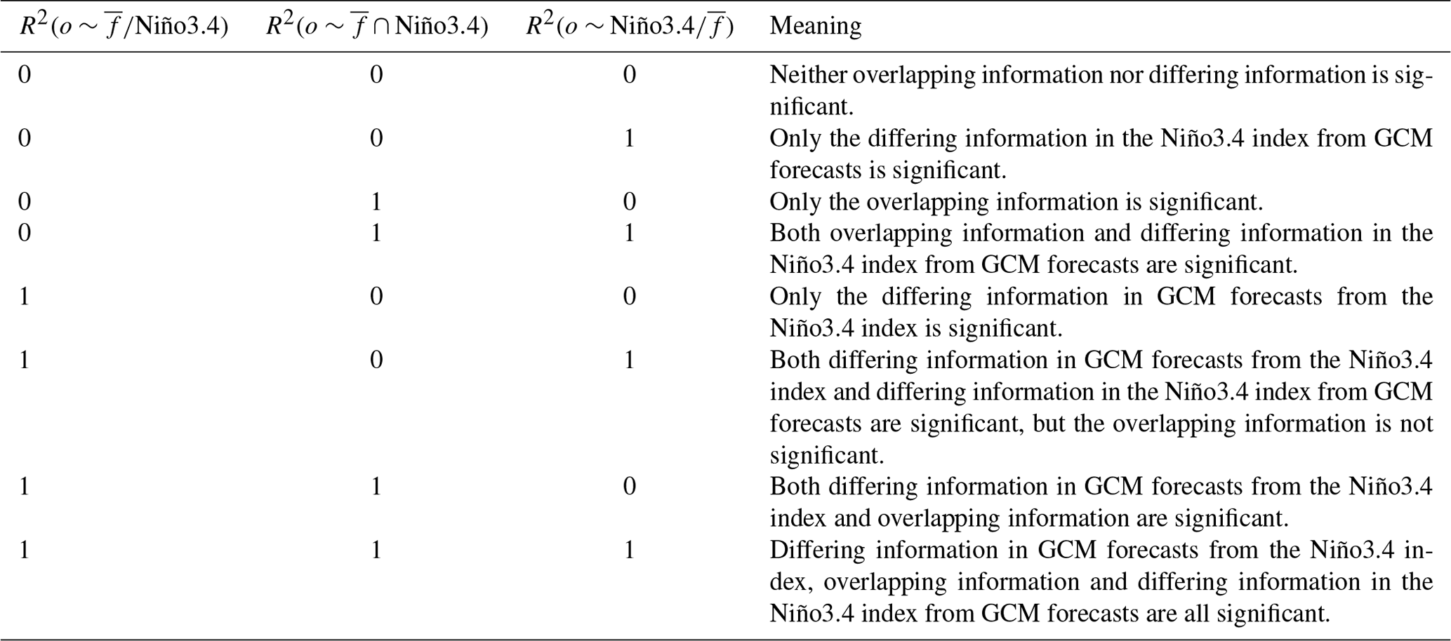
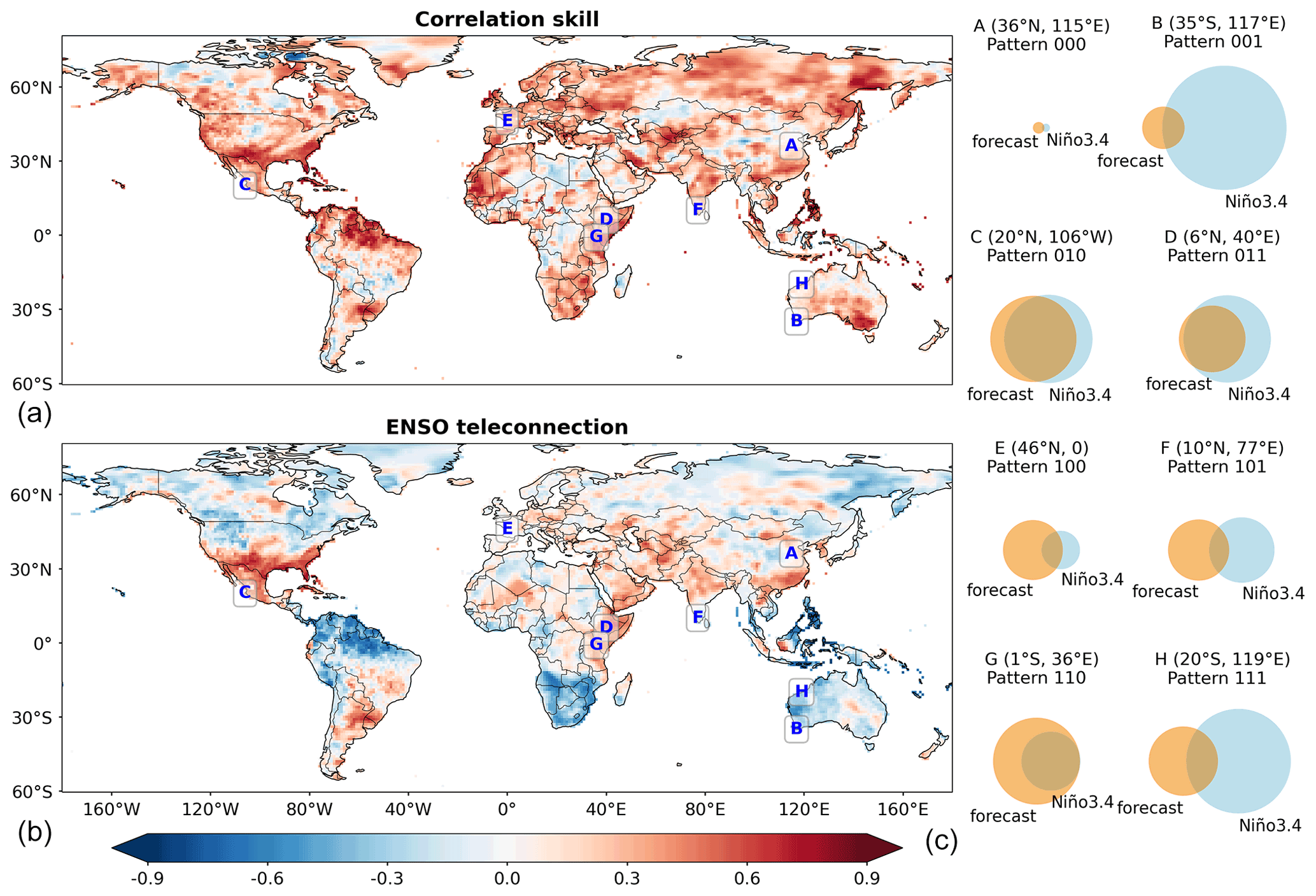
Figure 2 Spatial plots of correlation skill (a) and ENSO teleconnection (b) for global precipitation in DJF, and Venn diagrams (c) of overlapping and differing information for eight selected grid cells under the eight patterns.

The one type of overlapping information and the two types of differing information each have two cases of significance, i.e., significant or non-significant. Therefore, in Table 1, a three-digit number is devised to represent the results of significance tests. The first digit indicates the significance of $R^{\mathrm{2}}(o\sim \stackrel{\mathrm{‾}}{f}/\text{Niño}\mathrm{3.4})$, the second digit the significance of $R^{\mathrm{2}}(o\sim \stackrel{\mathrm{‾}}{f}\cap \text{Niño}\mathrm{3.4})$ and the third digit the significance of $R^{\mathrm{2}}(o\sim \text{Niño}\mathrm{3.4}/\stackrel{\mathrm{‾}}{f})$. As shown in Table 1, there are in total 8 ($\mathrm{2}\cdot \mathrm{2}\cdot \mathrm{2}$) patterns, with 1 representing a significant case and 0 indicating a non-significant case. The meanings of the eight patterns are illustrated in the last column of Table 1.

4 Results

4.1 Spatial plots of correlation skill and ENSO teleconnection

GCM forecast correlation skill and ENSO teleconnection for DJF are shown on the left-hand side of Fig. 2. The correlation skill is mathematically Pearson's correlation coefficient between the GCM forecast ensemble mean and observed precipitation. In the upper left part of Fig. 2, it is observed that the correlation skill is higher than 0.3 in a substantial number of grid cells around the world. This result indicates that the ensemble mean is generally indicative of observed precipitation; i.e., high values of the ensemble mean coincide with high values of observed precipitation and vice versa (Saha et al., 2014; Yuan et al., 2014; Cash et al., 2019). In the lower left part is ENSO teleconnection that mathematically represents Pearson's correlation coefficient between the Niño3.4 index and observed precipitation. Both positive and negative ENSO teleconnections are observed. For example, the teleconnection tends to be positive in southern North America, southeastern South America, southern China and eastern Africa, implying above-average precipitation in El Niño years but below-average precipitation in La Niña years, and it turns out to be negative in the northern part of South America, southern Africa as well as Southeast Asia; i.e., there can be below-average precipitation in El Niño years and above-average precipitation in La Niña years (Mason and Goddard, 2001; Emerton et al., 2017; Yang et al., 2018).

The SOCD method facilitates in total eight patterns to characterize the overlapping and differing information for the GCM forecast ensemble mean and the Niño3.4 index. As the Venn diagram in Fig. 1 is presented for the purpose of conceptual illustration, the right-hand side of Fig. 2 showcases the Venn diagrams generated from real-world data. The eight patterns in Table 1 are illustrated for eight grid cells selected from the left-hand side of Fig. 2. Grid cell A (36^∘ N, 115^∘ E) is under pattern 000: the areas of the circles that indicate the ratios of explained variance are rather small, implying little information on observed precipitation in GCM forecasts and the Niño3.4 index. By contrast, the areas of the circles are larger for the other seven selected grid cells, suggesting the existence of significant overlapping or differing information. For example, the significant overlapping information is highlighted in grid cell C (20^∘ N, 106^∘ W), the significant differing information in GCM forecasts from the Niño3.4 index is shown in grid cell E (46^∘ N, 0^∘) and the significant differing information in the Niño3.4 index from GCM forecasts is highlighted in grid cell B (35^∘ S, 117^∘ E).

The spatial distribution of the eight patterns is shown in Fig. 3 by applying the SOCD method and the bootstrapping significance test to all the land grid cells. Grid cells under pattern 000, which indicates poor GCM correlation skill and limited ENSO teleconnection, are in grey. On the other hand, it is noted that a considerable number of grid cells around the world are colored. That is, for the overlapping information and the two types of differing information, at least one of them is significant. From the left-hand side of Fig. 2, it can be found that positive correlation skill corresponds to positive ENSO teleconnection in southern North America and eastern Africa and that positive correlation skill corresponds to negative teleconnection over the northern part of South America, southern Africa and Southeast Asia. In the meantime, from Fig. 3 it can be observed that in these regions a considerable number of grid cells fall under patterns 010, 110 and 011, indicating the existence of significant overlapping information.

Figure 3 Spatial distribution of the eight patterns of overlapping and differing information.

4.2 Patterns of overlapping and differing information

The eight patterns serve as a link between correlation skill and ENSO teleconnection. Pattern 010 that is concentrated on the overlapping information is shown in Fig. 4. On the left-hand side of the figure are the results for grid cells under pattern 010 (the results for the other grid cells are masked). The overlapping information is significant in southern North America, where positive correlation skill (upper left part of Fig. 4) coincides with positive ENSO teleconnection (lower left part of Fig. 4). It is also significant in southern Africa and northern South America, where positive correlation skill and negative ENSO teleconnection coexist. As both correlation skill and ENSO teleconnection are mathematically Pearson's correlation coefficient, they can each be classified into three cases, i.e., significantly positive (P), non-significant (ns) and significantly negative (N) (Kirtman et al., 2014; Emerton et al., 2017; Huang and Zhao, 2022). On the right-hand side of Fig. 4, the Sankey diagram shows that 18.95 % of the global land grid cells exhibit pattern 010. For this pattern, 8.98 % of grid cells exhibit significantly positive correlation skill, 9.85 % non-significant correlation skill and 0.12 % significantly negative correlation skill. In the meantime, 3.77 % exhibit significantly positive ENSO teleconnection, 10.92 % non-significant ENSO teleconnection and 4.25 % significantly negative ENSO teleconnection.

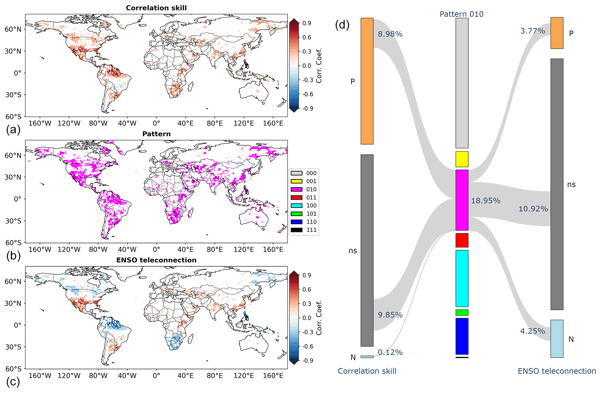
Figure 4 Illustrations of correlation skill (a) and ENSO teleconnection (c) under pattern 010 (b) and the Sankey diagram showing the percentages of grid cells under pattern 010 and the percentages of grid cells exhibiting significantly positive (P), non-significant (ns) and significantly negative (N) correlation skill/ENSO teleconnection (d). Grid cells under the other patterns are masked and therefore not shown in the spatial plots and the Sankey diagram.

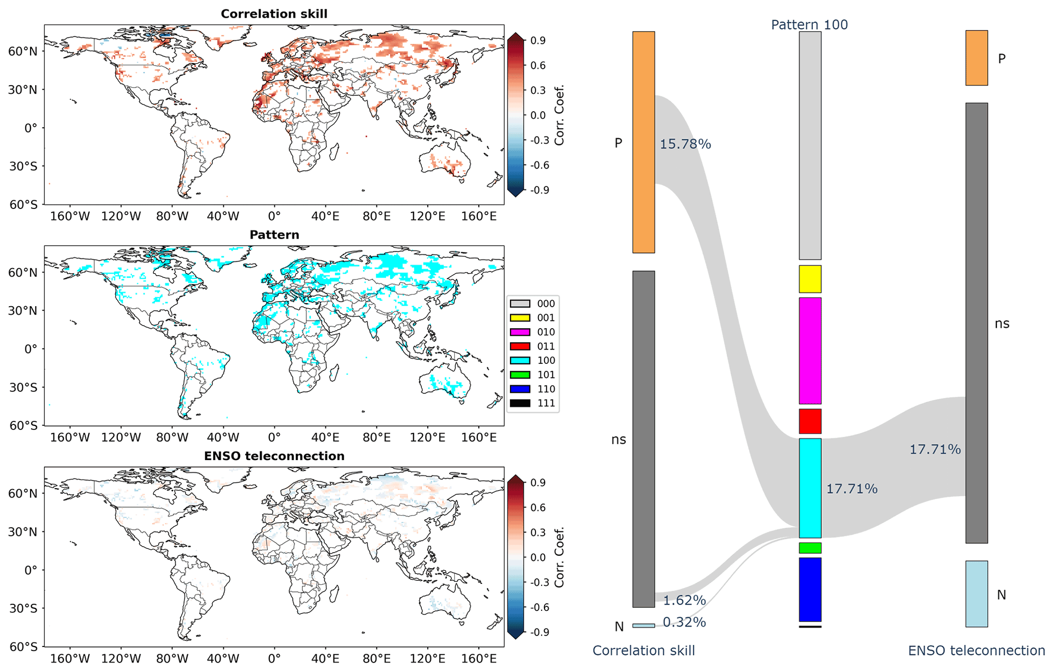
Figure 5 As for Fig. 4 but for pattern 100.

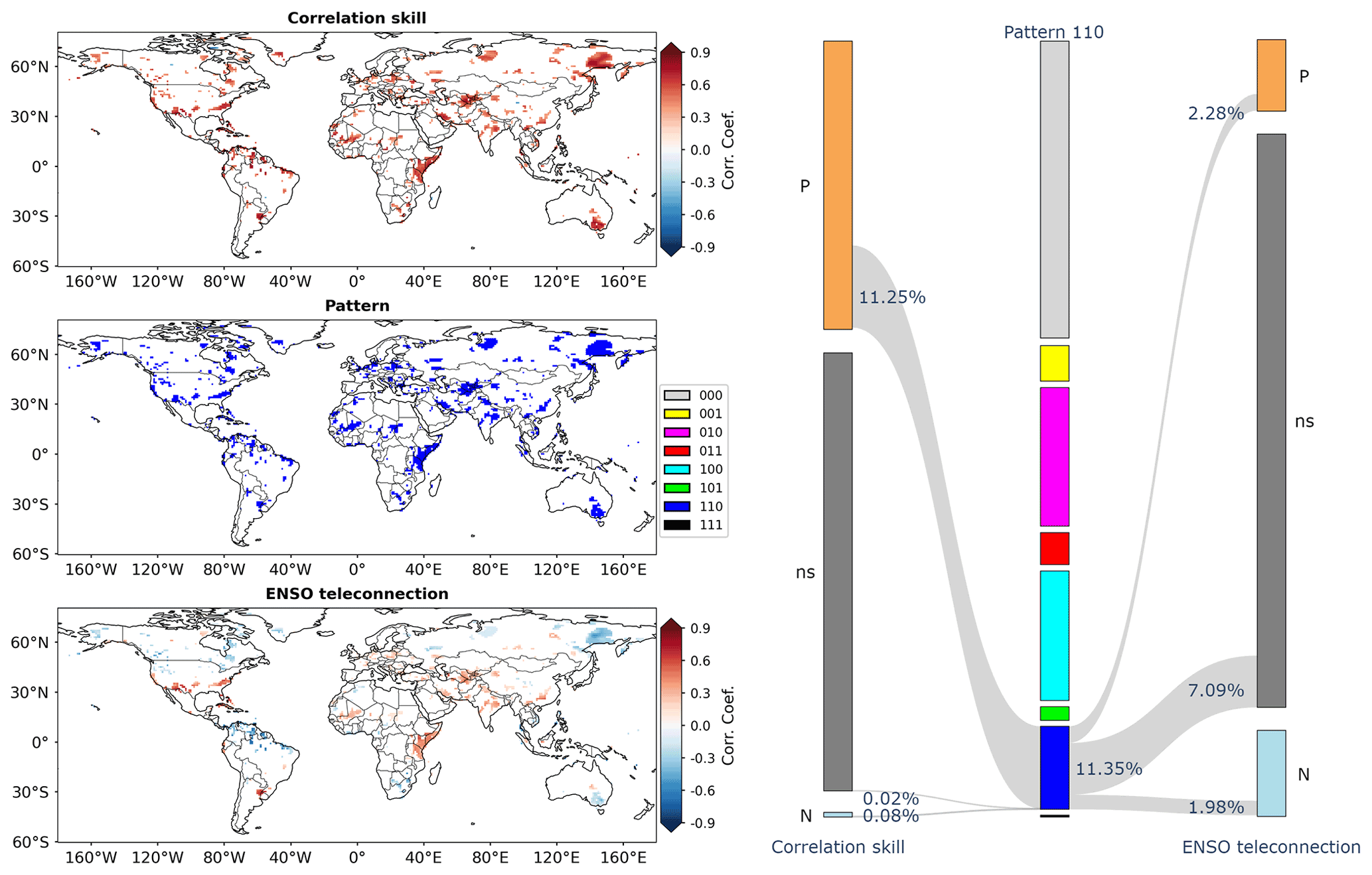
Figure 6 As for Fig. 4 but for pattern 110.

Figure 7 As for Fig. 4 but for pattern 001.

Figure 8 As for Fig. 4 but for pattern 011.

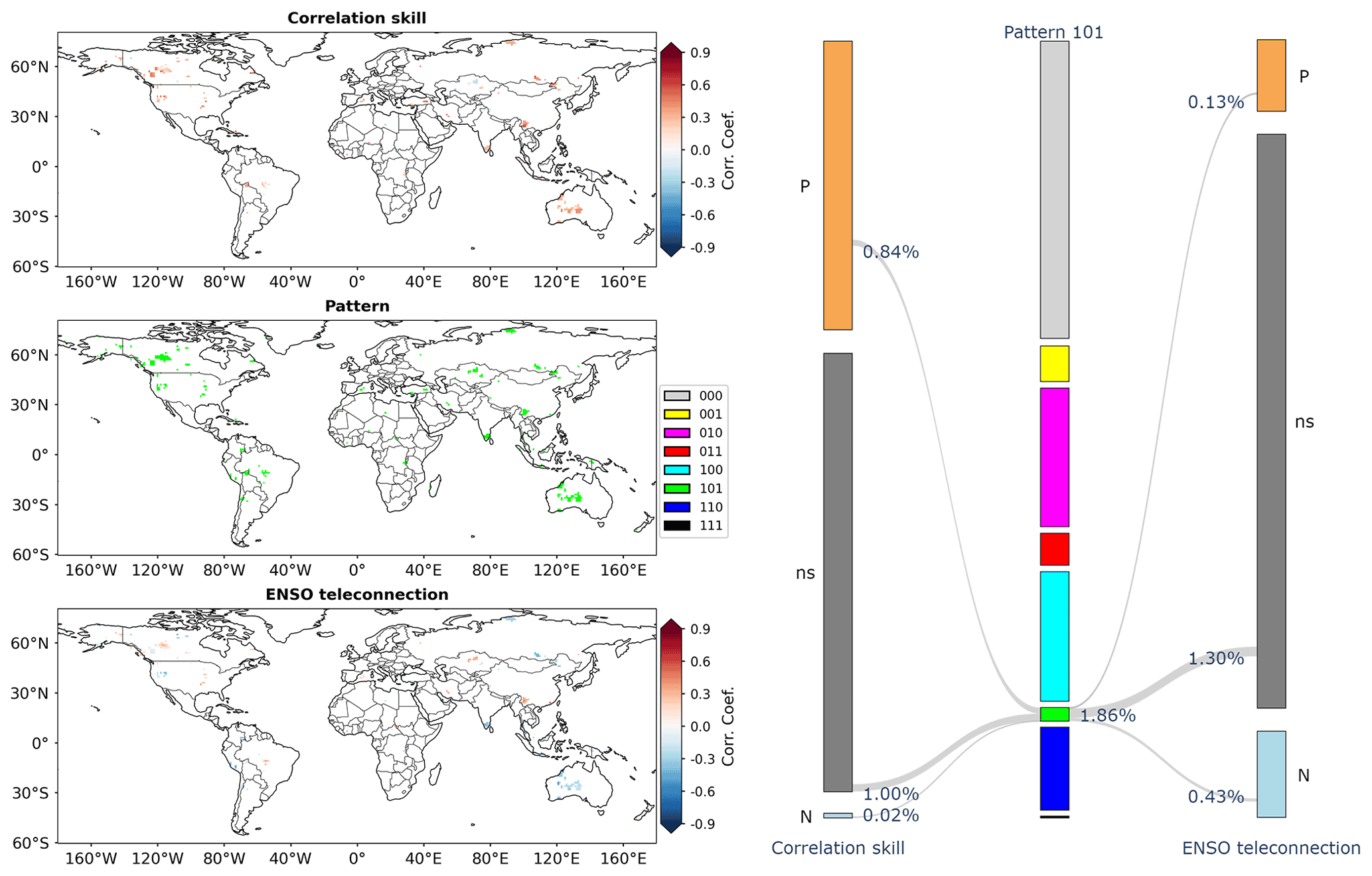
Figure 9 As for Fig. 4 but for pattern 101.

Figure 10 As for Fig. 4 but for pattern 111.

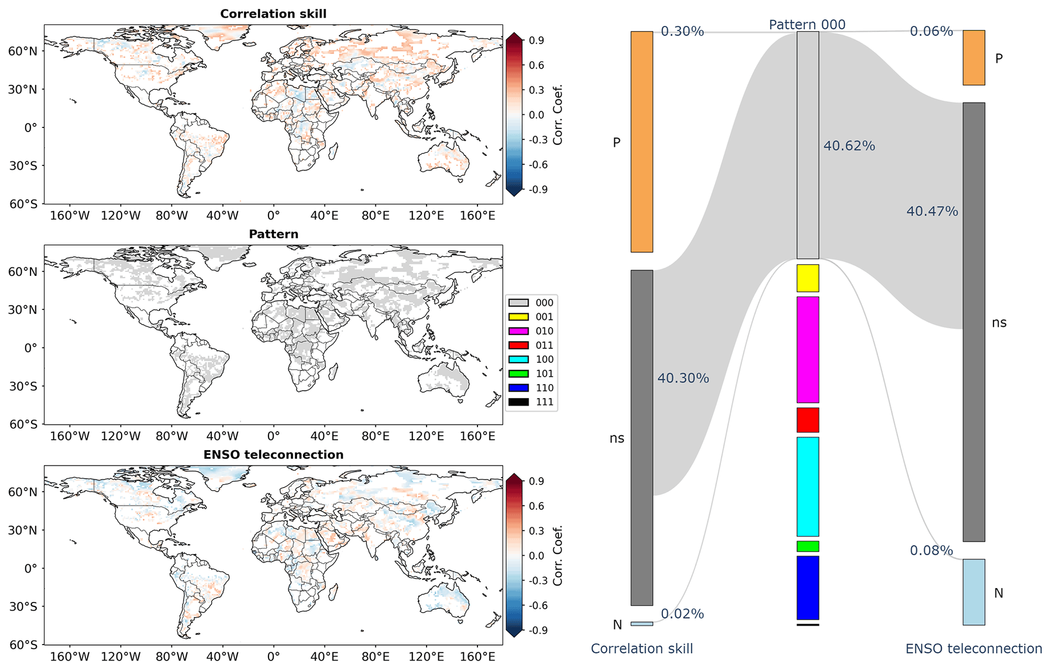
Figure 11 As for Fig. 4 but for pattern 000.

Pattern 100 that focuses on the significant differing information of global precipitation in GCM forecasts from the Niño3.4 index is shown in Fig. 5. From the left-hand side of the figure, it can be observed that this pattern (middle left part) tends to cover grid cells where correlation skill is around or above 0.3 (upper left part) but ENSO teleconnection is nearly zero (lower left part). This observation is confirmed by the right-hand side of Fig. 5. As can be seen, while the percentage of grid cells falling into pattern 100 is 17.71 %, most of them have significantly positive correlation skill (15.78 % in 17.71 %), and by contrast all of them exhibit non-significant ENSO teleconnection (17.71 % in 17.71 %). That is, the correlation skill is largely significantly positive but the ENSO teleconnection is generally neutral. These grid cells tend to be located in Europe and northern Asia, where the influence of ENSO is limited and skillful GCM forecasts can relate to other teleconnections such as the Arctic Oscillation and North Atlantic Oscillation (Hamouda et al., 2021).

Pattern 110 indicates that the overlapping information is significant and that the differing information in GCM forecasts from the Niño3.4 index is also significant. The implication is that, regarding global seasonal precipitation in DJF, GCM forecasts not only contain information that is contained in the Niño3.4 index, but also provide a considerable amount of additional information. On the left-hand side of Fig. 6, some grid cells under pattern 110 are observed in southeastern Australia, eastern Africa and northeastern Asia. Comparing Fig. 6 to Fig. 4, it is observed that some grid cells in southern North America, northern South America and southern Africa are under pattern 110, although many of them tend to be under pattern 100. Around the world, the percentage of grid cells falling into pattern 110 is 11.35 %. For these grid cells, correlation skill is predominantly significantly positive (11.25 % in 11.35 %) and, by contrast, ENSO teleconnection tends to be non-significant (7.09 % in 11.35 %).

Pattern 001 pays attention to the differing information in the Niño3.4 index from GCM forecasts. As shown in Fig. 7, this pattern covers 4.87 % of grid cells around the world. On the left-hand side of Fig. 7, it is worthwhile noting that a number of grid cells in western Australia exhibit significantly negative ENSO teleconnection but non-significant correlation skill. The implication is that therein GCM forecasts might fail to account for the information of ENSO teleconnection. On the right-hand side of Fig. 7, it is observed that most grid cells under pattern 001 have neutral correlation skill (4.86 % in 4.87 %) and that their corresponding ENSO teleconnection can be significantly negative (2.21 % in 4.87 %) or significantly positive (1.73 % in 4.87 %).

Pattern 011, shown in Fig. 8, indicates that both the overlapping information and the differing information in the Niño3.4 index from GCM forecasts are significant. Grid cells exhibiting this pattern tend to be scattered in parts of southern North America, northern South America, Southeast Asia and southern Africa. They account for 4.38 % of grid cells around the world. Among them, 1.72 % exhibit significantly positive ENSO teleconnection and 2.66 % significantly negative ENSO teleconnection. For these areas, the significant overlap suggests that a substantial amount of information in seasonal precipitation can be explained by both GCM forecasts and Niño3.4, while the significant differing information indicates the part that can only be explained by the Niño3.4 index.

Pattern 101 is shown in Fig. 9. It suggests that, at some grid cells, the overlapping information is not significant but that the two types of differing information are significant for both GCM forecasts and the Niño3.4 index. About 1.86 % of grid cells fall into this pattern.

Pattern 111 is shown in Fig. 10. It implies that, at some other grid cells, the overlapping information and the two types of differing information can all be significant. It is noted that only 0.26 % of grid cells around the world exhibit pattern 111.

Among the eight patterns, pattern 000 covers the most grid cells. The left-hand side of Fig. 11 shows that grid cells under pattern 000 generally exhibit non-significant correlation skill and non-significant ENSO teleconnection. This result is in sharp contrast to pattern 010, which indicates reasonable correspondence between correlation skill and ENSO teleconnection (Fig. 4), and to patterns 100 and 110, which suggest significantly positive correlation skill (Figs. 5 and 6). Overall, the percentage of grid cells under pattern 000 is 40.62 %. These grid cells predominantly exhibit neutral correlation skill (40.30 % in 40.62 %) and also neutral ENSO teleconnection (40.47 % in 40.62 %).

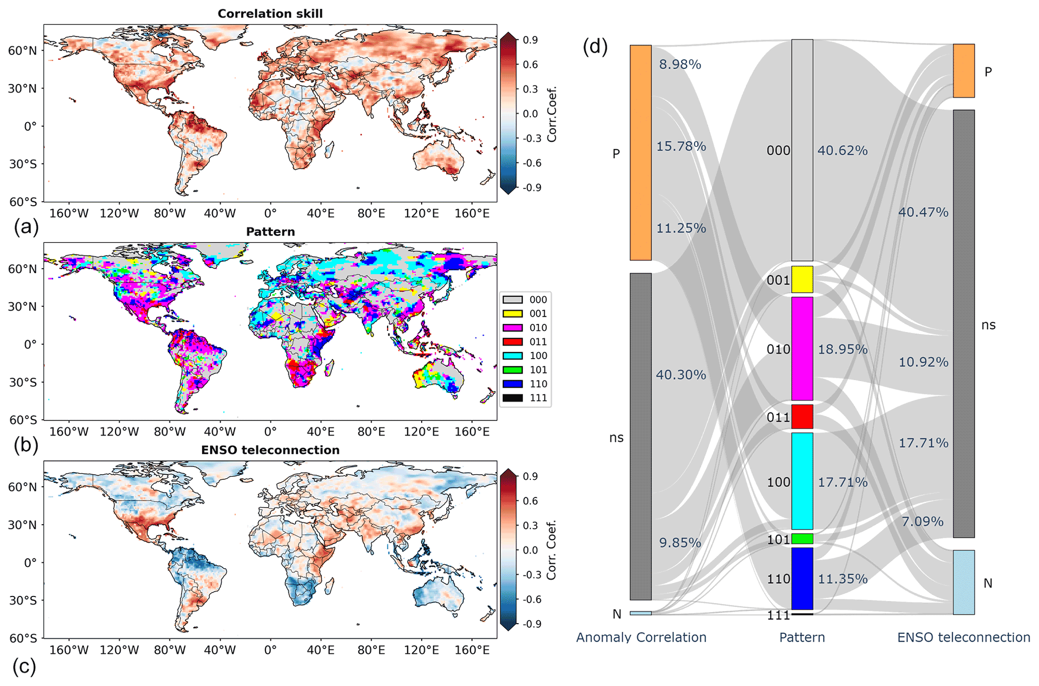
Figure 12 Spatial plots of correlation skill (a) and ENSO teleconnection (c) under the eight patterns (b) at the global scale and the Sankey diagram showing the percentages of grid cells exhibiting P, ns and N correlation skill/ENSO teleconnection (d).

4.3 Association of correlation skill with ENSO teleconnection

The results under the eight patterns are furthermore pooled in the analysis. From Fig. 12, it can be observed that the eight patterns serve as an effective link between correlation skill and ENSO teleconnection at the global scale. For the patterns that indicate significant information, the Sankey diagram on the right-hand side suggests that the percentage from highest to lowest is, respectively, 18.95 % for pattern 010, 17.71 % for pattern 100, 11.35 % for pattern 110, 4.87 % for pattern 001, 4.38 % for pattern 011, 1.86 % for pattern 101 and 0.26 % for pattern 111. More than half of the grid cells that exhibit significant correlation skill have significant overlapping information with Niño3.4, indicating considerable impacts of ENSO teleconnection on CFSv2 correlation skill.

GCM forecasts and the Niño3.4 index generally represent two different sources of information on global precipitation. In Fig. 13, GCM forecast correlation skill is plotted against ENSO teleconnection by using scatter plots. Figure 13a pools global land grid cells and employs the viridis heatmap to indicate point density. It can be observed that the correlation skill is largely positive and falls above the horizontal line. In addition, the heatmap suggests that the correlation skill tends to increase with the increase in positive ENSO teleconnection and also with the decrease in negative ENSO teleconnection. These results suggest that the skill of GCM forecasts benefits from the prominence of ENSO teleconnection since GCMs tend to capture the influences of ENSO on the variability of global precipitation (Saha et al., 2014; Khan et al., 2017; Delworth et al., 2020; Johnson et al., 2019; Becker et al., 2022).

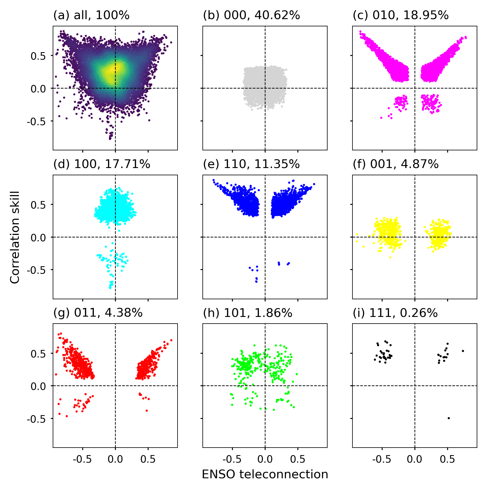
Figure 13 Scatter plots of the association of GCM forecast correlation skill with ENSO teleconnection at the global scale with the heatmap indicating the density of scatter points (a) and of the association of correlation skill with ENSO teleconnection under the eight patterns (b–i).

The subplots in Figs. 13b–i are arranged in descending order of the percentage of grid cells. Overall, close but divergent associations of correlation skill with ENSO teleconnection can be observed.

1. There exists significant overlapping information in GCM forecasts and the Niño3.4 index under patterns 010 (Fig. 13c), 110 (Fig. 13e), 011 (Fig. 13g) and 111 (Fig. 13i). It covers 34.94 % of land grid cells, i.e., 18.95 % (010) + 11.35 % (110) + 4.38 % (011) + 0.26 % (111), around the world. From the corresponding scatter plots, it can be observed that both correlation skill and ENSO teleconnection ought to be reasonably high to facilitate significant overlapping information.

2. There is significant differing information in GCM forecasts from the Niño3.4 index under patterns 100 (Fig. 13d), 110 (Fig. 13e), 101 (Fig. 13h) and 111 (Fig. 13i). It covers 31.18 % of global land grid cells, i.e., 17.71 % (100) + 11.35 % (110) + 1.86 % (101) + 0.26 % (111). Under these patterns, it is highlighted that the correlation skill tends to be higher than ENSO teleconnection. In particular, significantly positive correlation skill coincides with overall non-significant ENSO teleconnection under pattern 100 in Fig. 13d. Overall, these results imply that, apart from ENSO, GCMs account for other hydroclimatic teleconnections to produce skillful precipitation forecasts (Saha et al., 2014; Delworth et al., 2020; Lin et al., 2020).

3. There is significant differing information in the Niño3.4 index from GCM forecasts under patterns 001 (Fig. 13f), 011 (Fig. 13g), 101 (Fig. 13h) and 111 (Fig. 13i). It covers 11.37 % of global land grid cells, i.e., 4.87 % (001) + 4.38 % (011) + 1.86 % (101) + 0.26 % (111). Under these patterns, ENSO teleconnection is generally higher than correlation skill. Remarkable ENSO teleconnection coincides with overall non-significant correlation skill under pattern 001 in Fig. 13f. These results suggest that some ENSO teleconnection is still to be exploited by GCMs to improve precipitation forecast skill.

4. Neither the overlapping information nor the two types of differing information are significant under pattern 000. It covers 40.62 % of the grid cells. From Fig. 13b, it can be observed that either correlation skill or ENSO teleconnection is limited and that the corresponding scatter plot tends to cluster around the origin point. This result suggests that, despite limited ENSO teleconnection, GCM forecasts still have plenty of room for improvement.

5 Discussion

The SOCD method is furthermore applied to investigate the eight patterns considering the effects of seasonality, lead time, lag time and significance level. The additional results are presented in the Supplement. (1) The effect of seasonality is shown in Figs. S1 to S6 in the Supplement. It can be observed that regions exhibiting significant ENSO teleconnections vary by season (Figs. S1 to S3) and that the eight patterns remain effective in characterizing the overlapping and differing information (Figs. S4 to S6). (2) The effect of lead time is illustrated in Figs. S7 to S10 in the Supplement. At the lead times of 1 and 2 months, the percentage of pattern 010 remains the highest among the seven patterns other than 000. This result highlights the existence of significant overlapping information in DJF, particularly over southern North America, northern South America and southern Africa. (3) The effect of the lag time of the Niño3.4 index is illustrated in Figs. S11 to S14 in the Supplement. Compared to the concurrent teleconnection, the spatial distribution of the eight patterns tends to be similar for the monthly Niño3.4 index at the lag times of 1 and 2 months, with a slight increase in the percentage of pattern 000. This result confirms the temporal persistency in the Niño3.4 index (Yang et al., 2018). (4) The effect of the significance level is shown in Figs. S15 to S18 in the Supplement. As the significance level is reduced from 0.10 to 0.05 and furthermore to 0.01, the percentage of pattern 000 evidently increases, but the seven patterns that highlight significant overlapping and differing information remain.

The SOCD method is also extended to evaluate the overlapping and differing information under other GCM forecasts and hydroclimatic teleconnections. In the Supplement, Figs. S19 and S20 show the results for the CanCM4 forecasts generated at the Canadian Meteorological Center (CMC) (Merryfield et al., 2013). The CanCM4 forecasts seem to be less skillful in Europe but more skillful in the western part of Australia. Overall, the percentage of pattern 000 is slightly higher than that for CFSv2 forecasts. These results suggest that different GCM forecasts can be complementary to each other in different regions and that they can be combined to generate more skillful forecasts (Kirtman et al., 2014; Slater et al., 2019; Schepen et al., 2020). Figures S21 and S22 in the Supplement present the eight patterns for the Indian Ocean Dipole (IOD) (Cai et al., 2021). It can be observed that the percentage of pattern 010 is reduced from 18.95 % to 9.41 %, while the percentage of pattern 100 is increased from 17.71 % to 22.83 %. The indications are that CFSv2 forecasts exhibit less overlapping information with IOD and that there exists considerable differing information in CFSv2 forecasts from IOD teleconnection.

The correlation skill is one of the most popular measures of forecast skill owing to its simplicity in calculation and robustness to zero and missing values (Barnston et al., 2012; Yuan et al., 2014; Ma et al., 2016; Slater et al., 2019; Huang and Zhao, 2022). From spatial plots of correlation skill at regional and global scales, it can be observed where GCM forecasts are skillful and where GCM forecasts are not satisfactory (Ma et al., 2016; Slater et al., 2019; Delworth et al., 2020). Previously, it was observed that GCM forecasts tend to be skillful in regions subject to prominent influences of ENSO; accordingly, forecast skill is attributed to the effectiveness of GCMs in capturing ENSO-related climate dynamics (Kirtman et al., 2014; Slater et al., 2019; Lin et al., 2020). In this paper, the developed SOCD method not only confirms the significant overlapping information, but also highlights that there exists significant differing information in GCM forecasts from ENSO teleconnection for 31.18 % of global land grid cells and that there is significant differing information in ENSO teleconnection from GCM forecasts for 11.37 % of the grid cells. It is noted that the simple linear regression accounts for linear relationships. Nonlinear relationships between forecasts and observations are possible, and in the future nonlinear models can be adopted in the analysis of the overlapping and differing information (Strazzo et al., 2019; Schepen et al., 2020; Li et al., 2021).

6 Conclusions

While ENSO teleconnection has been conventionally used in the forecasting of regional precipitation and streamflow, GCM forecasts are increasingly available for hydrological applications. It is important to investigate to what extent emerging GCM forecasts provide “new” information compared to conventional ENSO teleconnection. The SOCD method developed in this paper addresses this issue through the mathematical formulations and numerical implementations of set operations. Specifically, the union operation quantifies the information of global seasonal precipitation contained in both GCM forecasts and the Niño3.4 index, the intersection operation derives the overlapping information of global precipitation in GCM forecasts and the Niño3.4 index and, furthermore, the difference operations illustrate two types of differing information, i.e., the differing information in GCM forecasts from the Niño3.4 index and the differing information in the Niño3.4 index from GCM forecasts. The significance tests of the three types of information facilitate in total eight patterns to disentangle the close but divergent associations of GCM forecast correlation skill with ENSO teleconnection. GCM forecasts and the Niño3.4 index generally provide two different sources of data for precipitation forecasting. While the existence of significant overlapping information suggests that they can provide some similar information, the existence of significant differing information highlights that the two data sources can also be complementary to each other. In the future, more efforts can be devoted to investigating more datasets of GCM forecasts and more hydroclimatic teleconnections to yield insights into the forecast skill of GCM forecasts and to facilitate applications of GCM forecasts to hydrological modeling and water resources management.