the Creative Commons Attribution 4.0 License.
the Creative Commons Attribution 4.0 License.
 | 26 Jan 2022
Aquifer recharge in the Piedmont Alpine zone: historical trends and future scenarios
Elisa Brussolo
Jost von Hardenberg
Giulio Masetti
Gianna Vivaldo
Maurizio Previati
Davide Canone
Davide Gisolo
Ivan Bevilacqua
Antonello Provenzale
Stefano Ferraris
The spatial and temporal variability of air temperature, precipitation, actual evapotranspiration (AET) and their related water balance components, as well as their responses to anthropogenic climate change, provide fundamental information for an effective management of water resources and for a proactive involvement of users and stakeholders, in order to develop and apply adaptation and mitigation strategies at the local level.
In this study, using an interdisciplinary research approach tailored to water management needs, we evaluate the past, present and future quantity of water potentially available for drinking supply in the water catchments feeding the about 2.3 million inhabitants of the Turin metropolitan area (the former Province of Turin, north-western Italy), considering climatologies at the quarterly and yearly timescales. Observed daily maximum surface air temperature and precipitation data from 1959 to 2017 were analysed to assess historical trends, their significance and the possible cross-correlations between the water balance components. Regional climate model (RCM) simulations from a small ensemble were analysed to provide mid-century projections of the difference between precipitation and AET for the area of interest in the future CMIP5 scenarios RCP4.5 (stabilization) and RCP8.5 (business as usual). Temporal and spatial variations in recharge were approximated with variations of drainage. The impact of irrigation, and of snowpack variability, on the latter was also assessed. The other terms of water balance were disregarded because they are affected by higher uncertainty.
The analysis over the historical period indicated that the driest area of the study region displayed significant negative annual (and spring) trends of both precipitation and drainage. Results from field experiments were used to model irrigation, and we found that relatively wetter watersheds in the northern and in the southern parts behave differently, with a significant increase of AET due to irrigation. The analysis of future projections suggested almost stationary conditions for annual data. Regarding quarterly data, a slight decrease in summer drainage was found in three out of five models in both emission scenarios. The RCM ensemble exhibits a large spread in the representation of the future drainage trends. The large interannual variability of precipitation was also quantified and identified as a relevant risk factor for water management, expected to play a major role also in future decades.
- Article
(18291 KB) - Full-text XML
-
Supplement
(169 KB) - BibTeX
- EndNote


Water is a crucial resource, intrinsically linked to society and culture development, food and energy security, well-being, environmental sustainability and poverty reduction. However, several factors, including urbanization, population growth, land use and soil consumption, and industrial and agricultural development, endanger water resource sustainability in terms of availability, quality, management and demand (IPCC, 2014; WWAP, 2015). Groundwater resources represent about 97 % of liquid freshwater resources on Earth (WHO, 2006; Healy, 2010) and play a key role in water supply and proper preservation of ecosystems (WWAP, 2015). Groundwater resources help to maintain river discharges and, together with surface freshwaters, are accounted for in water budget considerations at the river basin scale (Rumsey et al., 2015). The hydrological connection between groundwater and surface water is primarily controlled by (1) the driving force generated by the hydraulic gradient between groundwater and surface water and (2) the permeability degree of the aquifer in comparison to a streambed (i.e. different hydraulic conductivity) due to the geological context (Lasagna et al., 2016; Epting et al., 2018). Groundwater and surface water interaction is influenced by both local and regional regimes (Epting et al., 2018). Local interaction could be very complex, and different methods were developed to quantify this interaction in different locations (Bertrand et al., 2014; Kalbus et al., 2006). Groundwater resources are of utmost importance for their mitigation effects during dry periods, and their reduction can impact the whole hydrological cycle. Groundwater is a fundamental natural resource that acts as a reservoir from which good-quality water can be collected for drinking purposes, requiring few purifying treatments compared to surface water. Climate change influences several components of the water cycle, including groundwater resources, causing a lowering of piezometric levels due to discharge modifications as a result of snow retention reduction, changes in precipitation regimes and potential evapotranspiration that increases with increasing temperatures. In Alpine regions, shorter and thinner snowpack will decrease late spring flows, while the air temperature rise will increase stream flows in autumn and winter due to trading of snowfall for rainfall (Confortola et al., 2013), leading to a shift of groundwater recharge from summer to winter, as evaluated by CH2018-Project-Team (2018) and Epting et al. (2021) in Switzerland.
Surface water and pollutants infiltration, together with over-exploitation of wells, can further deplete groundwater resources, triggering the competition between irrigation and potable uses. While the degradation of water quality mostly depends on land use and saltwater intrusions into coastal groundwater (Jiménez Cisneros et al., 2014), climate change also may affect, either directly or indirectly, the quality of groundwater resources. Temperature impacts biological, chemical and physical properties of groundwater resources (Epting et al., 2021), even if the increase of air temperature is not necessary directly correlated with groundwater temperature increase. In fact, this correlation depends on the intrinsic properties of aquifers, on local and regional spatio-temporal scales and on different anthropic inputs (Epting et al., 2021; Bastiancich et al., 2021). Moreover, the interaction between surface water and groundwater flow systems influences the water chemistry (Lasagna et al., 2016), since in areas where rainfall intensity is expected to increase, pollutants will be increasingly washed from soils to water bodies (IPCC, 2007). Finally, water-level changes are a key indicator that flow patterns are changing and that low-quality water may be mobilized (Moench et al., 2003).
Climate change also exacerbates the risks associated with changes in the distribution and availability of water resources (Jiménez Cisneros et al., 2014), with consequences for water-demand management and infrastructural system planning (van der Gun, 2012). In this framework, assessing climate change impacts on Integrated Urban Water Management (IUWM), considering a worsening of pre-existing conditions and/or an occurrence of new hazards or risk factors and planning climate change adaptation strategies are fundamental challenges that IUWM is expected to face in the near future, using an integrated approach based on prevention, preparedness and risk assessment. To this end, an appropriate proactive engagement of stakeholders is needed, in order to develop and apply adaptation and mitigation strategies quantified and driven by state-of-the art climate information and projections.
The Alps and the Mediterranean area are recognized as two climate hotspot regions (IPCC, 2014), showing amplified climate change signals and associated environmental, social and economical impacts. Future projections for the Italian territory, in particular, show an increase of high precipitation intensity, typically distributed in more intermittent events, together with an increase of the duration of dry periods (Desiato et al., 2015). However, in north-western Italy, these trends are not clear, and they are very site-dependent (Baiamonte et al., 2019). In a recent paper analysing European floods, in Piedmont almost no precipitation trend emerged, with the exception of the Dora Riparia valley, where precipitation is declining (Blöschl et al., 2019). Another recent work shows the differences in freshwater trends between central and southern Europe (Gudmundsson et al., 2017). In fact, Italy is a climatic bridge between the Mediterranean and the inland European climate (Libertino et al., 2019), and in Piedmont there are mountains 4000 m high at just 160 km distance from the Mediterranean Sea.
Northern Italy is also a bridge between areas where actual evapotranspiration is mainly soil-moisture-limited (Mediterranean) and areas where it is energy-limited (central Europe).
For precipitation, the transient development of the impingement of cold fronts on the Alps induces a wide range of mesoscale phenomena. On the one hand, when the Alpine chain is subject to a southerly flow of moist and relatively warm air from the Mediterranean Sea, very intense precipitation episodes can take place, such as the Piedmont flood in November 1994. The Piedmont lowlands act as a natural trap for moist airflows from the south-east, particularly in autumn. On the other hand, northerly flows lead to dry weather, particularly in winter (Pradier et al., 2002). Most relevant rainfall and snowfall episodes, including extreme events, are thus due to southerly flow.
For water management, the IUWM in Italy is geographically organized into local districts (called “ATO” – Ambiti Territoriali Ottimali, which translates into “Optimal Territorial Divisions”), whose domains were defined based on various criteria, either administrative boundaries or physical ones, including river basin boundaries (Legislative Decree No 152/2006, as further amended). The boundaries of these districts mostly coincide with administrative borders; in the Piedmont region, the Turin metropolitan area represents local district ATO3, where the IUWM is provided by Società Metropolitana Acque Torino (SMAT). This is a wide and geographically complex area, and SMAT exploits many and diverse supply sources, with groundwater resources representing about 80 % of the whole water supply in terms of volume available to SMAT.
It is therefore important to evaluate the balance between precipitation and actual evapotranspiration (AET) and their related spatial and temporal variabilities. Several studies can be found in the literature which evaluate the impacts of climate change on groundwater resources, e.g. Jiménez Cisneros et al. (2014) and Taylor et al. (2013).
Recharge varies in space and time, and it is difficult to measure directly; therefore a comprehensive understanding is lacking. In this paper, we define recharge as the difference between precipitation and actual evapotranspiration. This simplification follows a recent review paper, where mesoscale is defined as the ideal scale for simulating the effect of climate change on recharge, and precipitation is mentioned as the largest source of recharge variability (Smerdon, 2017). Moreover, in a recent study, considering several wells located in nine regions of the central and north-eastern United States, the recharge (evaluated as drainage from the lowest model soil layer) was shown to be compatible with observed monthly groundwater storage anomalies and month-to-month changes in groundwater storage (Li et al., 2015). In the selected study area, a recent study commissioned by the Water Department of the Piedmont Region shows that the recharge areas of the deep aquifers occur in the high plain sectors, close to the Alps (Regione Piemonte, 2018b; De Luca et al., 2020), justifying our choice to avoid river-fed recharge. A new global dataset encompassing more than 5000 locations has shown that precipitation amounts and seasonality of temperature and precipitation are the most important variables (Moeck et al., 2020; Condon et al., 2020). Epting et al. (2021), in a recent paper on Swiss alluvial aquifers, underline the importance of both spatial and temporal variability in recharge related studies carried out in a region close to our study area. Regarding spatial variability, Pangle et al. (2014) identified drainage as a proxy for recharge in a controlled mesocosm. Their results highlighted the potential for local interactions between temperature, vegetation and soils to moderate the hydrological response to climate warming. The importance of soil and vegetation was also underlined by Condon et al. (2020). The outputs of the Pangle et al. (2014) study show that AET decreased in summer because of soil moisture shortage. This result is due to the fact that precipitation is out of phase with the growing season cycle, and irrigation is operated only for reproducing natural rainfall events. At the yearly timescale, they did not find a reduction of AET in their evaluation of trends.
Regarding temporal variability, interannual variability also plays a major role in groundwater recharge, and it is critical for water managers. Masbruch et al. (2016) have shown how quasi-decadal large groundwater recharge events can be important for replenishing the aquifers. These events are characterized by large precipitation (both rainfall and snow water equivalent) and by below-average seasonal temperatures.
Also, the effects of climate change are not all in the same direction. In a study using 16 global climate models (GCMs), a considerable uncertainty in both the magnitude and direction of recharge changes was shown for 2050 year projections in different parts of the High Plains (Crosbie et al., 2013). A more recent study has revealed variability in both direction and magnitude of hydrological changes for the Great Lake basin of North America, with a combination of different regional climate models (RCMs; Persaud et al., 2020).
Konapala et al. (2020) reported at the global scale an increase in annual mean evaporation over the land surface, attributed to the increase in temperature. They deal with water availability as the difference between precipitation and actual evapotranspiration. In this paper we call this quantity drainage, as a proxy for recharge, computed by the soil model in each pixel, without modelling both runoff and the underlying aquifer flow. The other terms of water balance have more uncertainty and probably lower impact: soil water storage is small, river runoff has scattered measurements and complex process modelling and subsurface flow always shows large uncertainties associated with its estimation (Healy, 2010).
In this paper we develop a stakeholder-driven interdisciplinary research study, where scientists in atmospheric/climate research and hydrologists work together with agricultural and soil scientists and experts from a water utility to quantify the role of groundwater, focusing on an area providing water to about 2.3 million people. This area is characterized by a very large spatial precipitation and air temperature variability, owing to the proximity of high mountains and of the sea.
The main research questions, relevant also for other regions worldwide, are as follows: (a) can the water balance show a significant trend only because of a significant trend in AET? Is also a significant trend in precipitation necessary? (b) How different are water balance trends in three different parts of the area, namely a drier west–east-oriented mountain area, a wetter mountain area and a mostly irrigated agricultural area? In fact, in about 7000 km2 there are quite different situations, the former two with an impact of snow versus rain and anticipated snowmelt trends and the latter with a AET temperature increase compensation with irrigation. (c) To what extent are the spatial variability and trends observed in the past 60 years expected to undergo changes during the next 30 years?
We evaluate the temporal variability and the trends of the water balance terms, estimating the quantity of groundwater resource available for drinking water supply in the water catchments of the area managed by SMAT. The analyses are performed at both the quarterly and the hydrological year timescale, for both past and future conditions, analysing a historical climate dataset for the period 1959–2017 and future projections from regional climate model RCA4 RCM simulations up to 2050, in order to be compliant with relatively short-term water management objectives.
The expected results will form a knowledge basis for operational indications and will be useful to characterize future groundwater resources availability in other border areas between Mediterranean and continental climate, especially where the water resource is subject to multiple anthropogenic pressures. This paper represents a scientific contribution to the management and the governance of water resources and water supply that could be applied worldwide, through, for example, the implementation of scientifically driven guidelines and strategic agendas on water supply and water policies.
2.1 Study area
Many foothill zones in the Alps and Apennines contain aquifer systems of strategic interest for water supply, especially for drinking purposes (Doveri et al., 2016). In this framework, the aquifer system extending in the foothill plain located between the western Alps and the Turin hills represents one of the most significant and studied groundwater bodies in the Piedmont region (Raco et al., 2021).
This study area, within the administrative borders of the Turin metropolitan area (encompassing the entire territory of the former Province of Turin), has a complex orography and is surrounded on the western and northern sides by the Alps (with elevation peaks higher than 4000 m above sea level at the border with the Valle d'Aosta region) and on the eastern and southern sides by hills and plains. Precipitation in the study area is characterized by relatively high spatial and temporal variability (yearly total ranging from about 500 mm in the plain to 2000 mm for high-elevation gauges). The study area, in fact, is prone to topographically induced precipitation and is exposed to the inflow of moisture-rich air from the Mediterranean Sea (Ciccarelli et al., 2008). It is also an area characterized by the occurrence of relatively long dry periods, up to 6.4 d on average during winter (Agnese et al., 2012; Baiamonte et al., 2019).
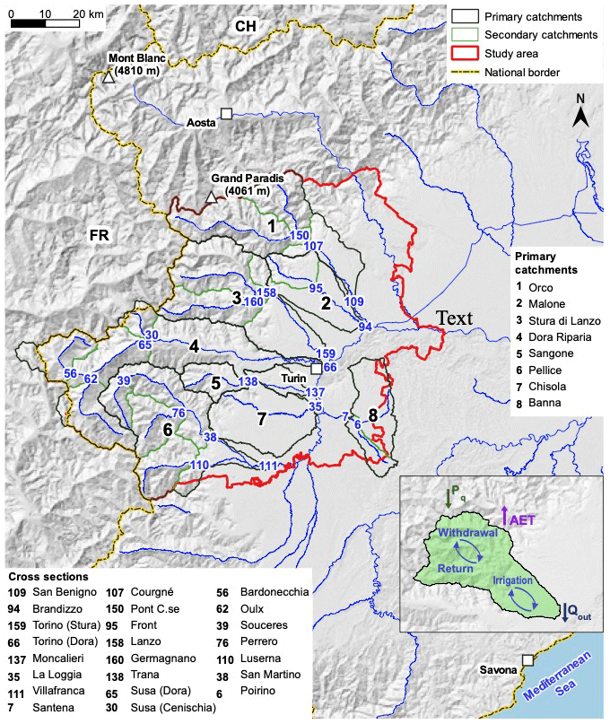
Figure 1The study area including river catchments and sub-catchments. Illustration of the water balance terms at the catchment scale is shown in the inset. Topographic shading is based on DEM data from the “Progetto Risknat – Base topografica transfrontaliera, ARPA Piemonte” (http://webgis.arpa.piemonte.it/ags101free/rest/services/topografia_dati_di_base/Sfumo_Europa_WM/MapServer, last access: 14 August 2020).
Owing to its hydrogeological features (see also the rivers system shown in Fig. 1), the foothill aquifer systems generally sustain the infiltration of both local rainfall and stream water originating from mountain catchments. These systems are highly sensitive to variations in meteoclimatic variables, first of all in precipitation regimes.
2.2 Water balance terms
In this paper we refer to water balance as the balance between water inputs and outputs at the catchment scale, as schematically shown in Fig. 1.
Given the timescales of interest and the uncertainties inherent in some terms of the water balance equation, in this study the standard formulation of this equation has been simplified, including precipitation, actual evapotranspiration (AET) and drainage (obtained by subtracting AET from the sum of rainfall and snowmelt), which is used as a proxy for the groundwater recharge. This approach is common to other studies, and many of them (Healy, 2010) do not make a distinction between drainage and groundwater recharge. This choice has also been discussed in the Introduction. Also, in the study area, measured river flow data cover a temporal interval shorter than 2 decades (2000–2017), not allowing robust regressive models to be built to be able to estimate deep percolation outside the time interval of data availability. Regarding the time step of calculation, the daily scale is recommended because of precipitation intermittency, in order to avoid the underestimation of drainage and recharge (e.g. Healy, 2010). Therefore in this work the computation is done at the daily scale in the soil column, and results are then aggregated at the yearly and quarterly timescale and, spatially, at the catchment scale.
The daily soil model will be described later in the text. The yearly catchment water balance can be simplified as follows (Healy, 2010):
where Pq represents the sum of liquid precipitation (rainfall) and snowmelt, AET the actual evapotranspiration and Qout the drainage. Surface and subsurface catchments are assumed to be coincident as they are bounded by the border mountain divide (De Luca et al., 2020). Storage variations in time are disregarded because the control volume is composed of vadose zone soil columns, with an aggregation of results at the quarterly and yearly timescale. The soil model presented in the following is used to calculate AET and Qout in each pixel at the daily timescale.
To account for the different ground characteristics and variations, together with the physical description of the hydrological processes, all the water balance variables (except for output discharge) must be first evaluated at a fine spatial resolution and then aggregated (i.e. upscaled) at watershed level. To this end, a horizontal spatial resolution of 250 m was considered to be a good compromise between the necessity of high resolution and the computational resources required: the study area was discretized into a grid of 652×521 pixels.
The model takes into account the effects of irrigation on the value of AET. However, input and output irrigation terms in surface and groundwater balance are assumed to balance out at the catchment level. Also, industrial water withdrawals do not change the water balance at the watershed scale because they give back the captured water at short distance, performed mostly for hydroelectric energy production.
The contribution of glacier and permanent snow melting can be disregarded because it is very small in comparison with the catchment areas. However the evaluation of snowmelt from the snowpack is quite important as it represents the amount of daily snow equivalent contributing to the water balance. In fact, as outlined in the review by Taylor et al. (2013), at high altitudes, increasing temperatures lead to less snow accumulation and earlier snowmelt and to more winter precipitation in form of rain.
To this end, as a first step, air temperature was used to distinguish between snowfall (Ps) and rainfall (Pr) (DeWalle and Rango, 2008): for temperatures lower than or equal to −2 ∘C, all the precipitation amount can be considered to be snowfall, while for temperatures higher than or equal to 5 ∘C, all the precipitation amount can be considered to be rainfall. For temperatures between −2 and 5 ∘C, rainfall and snowfall amounts were linearly interpolated, in order to break down the different percentages of precipitation type. The resulting snowfall Ps was used as an input to a simple bucket model in each pixel, used to integrate the storage of snow on ground, S. The daily snowmelt, Nf, was subtracted from the same bucket, and it was evaluated using the method by Zeinivand and Smedt (2009), where the melted snow is a function of the difference between the daily mean temperature Tmean and melting temperature T0 (0 ∘C) and of the rainfall amount (Pr evaluated in mm d−1), as follows:
where krain (rainfall melt-rate factor) and ksnow (melt-rate factor) are fixed parameters. The same values as in Zeinivand and Smedt (2009) were used: krain=0.0757 ∘C−1 and ksnow=3 mm d−1 ∘C−1.
A correct evaluation of the water balance allows for a reliable estimation of water availability. To this end, the following chain was applied in the study area:
-
identification and retrieval of the daily meteoclimatic (i.e. temperature and precipitation) data;
-
regridding of the meteoclimatic and hydrological data at the spatial resolution required by the hydrological model, namely a square 250 m grid;
-
setting up of a mathematical model that accounts for soil–vegetation–atmosphere interactions and provides actual evapotranspiration estimates (see Sect. 2.3).
Observational and reanalysis datasets have been used to obtain meteoclimatic data for the period 1959–2017, as described in Sect. 3, while for the assessment of future water balance scenarios, climate projections of temperature and precipitation were used (see Sect. 4).
In order to be compliant with management objectives for strategic long-term planning, the input datasets, available at daily resolution (see Sect. 3), were aggregated to quarterly and yearly timescales using the definition of hydrological year (the first quarter includes January, February and March (JFM), the second April, May and June (AMJ), the third July, August and September (JAS) and the fourth October, November and December (OND)). The hydrological year, N, starts on 1 October of year N−1 and ends on 30 September of year N. During the hydrological year, a complete snowfall melting occurs, making the breakdown of precipitation between rainfall and melted snow negligible. At high altitudes, this melting is not complete, and the annual variability entails the fluctuation of snow on the ground from one (hydrological) year to the following one. This phenomenon is limited to the highest peaks and is relevant only for limited areas. For this reason, for evaluations at the yearly timescale, Pq was assumed to be equal to the total average yearly precipitation.
2.3 Soil water model
A simple bucket soil water model was developed in order to estimate AET values at the daily scale for each 250 m × 250 m pixel of the study area. The soil is schematized with seven different layers of increasing thickness with depth, similar to the FAO56 model (Allen et al., 1998). The water inputs for the model are precipitation (sum of rainfall and melted snow) and irrigation, if any. The outputs are AET and drainage (sum of runoff and deep percolation). The distinction between runoff and deep percolation is not included in the model, as well as the modelling of capillary rise.
For each layer, the bucket equation is as follows:
where Pq is rainfall plus snowmelt, I* is irrigation, Qout is drainage, AET is actual evapotranspiration and ΔS is the variation of water storage in the soil per day. In a bucket model (as discussed by Baudena et al., 2012, in their paper focused on the same area in north-western Italy) water can be lost via evapotranspiration or evaporation and flow downwards between layers via deep percolation, as a function of soil water content of each layer: if it exceeds field capacity, the water surplus percolates into the layer immediately below.
2.4 Actual evapotranspiration computation
As reported by the Fifth Assessment Report of the IPCC (IPCC, 2014), a rise in greenhouse gas concentrations is associated with reduced soil moisture in Northern Hemisphere mid-latitude summers. This is the result of higher winter and spring evaporation, caused by higher temperatures and reduced snow cover, and of lower rainfall inputs during summer. Regarding the effects on recharge of managed agrosystems, Taylor et al. (2013) state that changes in surface energy budgets are associated with enhanced soil moisture from irrigation. The widespread use of irrigation in most parts of the Po Valley plain cancels out the dampening role of AET soil moisture limitation. At the same time, roughly half of the surface of the study area is covered by mountain grasslands and non-irrigated areas, where moisture limitation can play an important role.
The actual evapotranspiration, AET, was calculated starting from potential evapotranspiration, PET, then reduced by considering the actual soil water content, obtained from the bucket soil model for each layer, with AET of each day being the sum of the depletions from the single layers. PET was calculated with the model of Hargreaves and Samani as in Allen et al. (1998), using daily maximum and minimum air temperature data from the regional dataset described in Sect. 3.1 and extraterrestrial radiation modelled as in Aguilar et al. (2010). Also, the reduction of evapotranspiration (from PET to AET) due to actual soil water content was modelled using the coefficients Kc and Ks related to crop and soil respectively according to Allen et al. (1998), comparing the modelling results with real-world measurements at different sites (Raffelli et al., 2017).
The soil water model reproduces the data in the case of no irrigation very well. However, a relevant contribution of irrigation, especially for highly water-demanding crops such as maize, can increase the AET term of the water balance. These water-demanding crops are quite widespread in the study area (about 750 km2), and therefore a novel procedure reproducing agricultural irrigation techniques was implemented in the soil water model. This module is based on previous research in three farms (Canone et al., 2015, 2016), reproducing the farmers' decision rules and tuned in order to obtain irrigation events similar to the observed ones.
3.1 Temperature and precipitation
The past and present precipitation and temperature data necessary to force the hydrological model employed in this study were derived from the Regional Environmental Protection Agency of Piedmont (ARPA Piemonte) databases. In particular they have been extracted from the OI (optimal interpolation) dataset (in italian, ARPA Piemonte, 2010a). This dataset provides cumulative daily precipitation and maximum and minimum daily temperature at a spatial resolution of 0.125∘ longitude–latitude (corresponding to ∼12 km) over the entire Piedmont region, for a time period extending from 1959 to 2017. The OI dataset was obtained by interpolation of in situ observations collected by the Hydrographic Office network and by the network of the ARPA telemetry stations through the technique of optimal interpolation, which allows data to be obtained on a regular grid, homogenizing observational data from different measurement networks and sources (ARPA Piemonte, 2010b). A preliminary quality check of the OI data revealed the existence of days (all referring to years before 1990) for which the minimum temperature showed a higher value than the maximum temperature, probably owing to issues in the data acquisition. These data were excluded from the analysis and replaced by new values obtained through linear interpolation in time, rather than in space, in order not to smooth the orographic information inherent in the original OI dataset.
The OI dataset provides a set of meteorological variables at a coarser spatial resolution than that required to describe the small-scale hydrological processes and to accurately estimate the water balance terms, calling for the application of interpolation and downscaling techniques. After re-projecting the OI temperature and precipitation data into a WGS84/UTM zone 32 N coordinate system useful for the subsequent analyses, they were further interpolated at the finer resolution of 250 m over the domain of interest (xmin=304 250 m, xmax=434 500 m, ymin=4 951 750 m, ymax=5 094 750 m). The conversion was preceded by a preliminary bilinear interpolation of the OI dataset, in order to produce an intermediate higher resolution dataset at a resolution of 0.001∘ latitude–longitude and to avoid artefacts when re-projecting into UTM coordinates. Post-processing was performed using GDAL (Geospatial Data Abstraction Library; v. 2.1) and CDO (Climate Data Operators; v. 1.7.0) software.
A further adjustment to account for orographic effects was applied to maximum and minimum temperature data, using the environmental lapse-rate correction coefficients derived for the Alpine region by Rolland (2003), shown in Table 1. Figure 2 shows an example of orographic correction (panel b) applied to a maximum temperature field (panel a) for a selected day (1 January 2009). The orography of the study area is shown in the right panel, based on a 90 m resolution digital elevation model (DEM) derived from the SRTM (Shuttle Radar Topography Mission) project (Jarvis et al., 2008), interpolated at 250 m.
Table 1Average climatological monthly adiabatic lapse rate from Rolland (2003) for the Alpine region (expressed in K km−1).

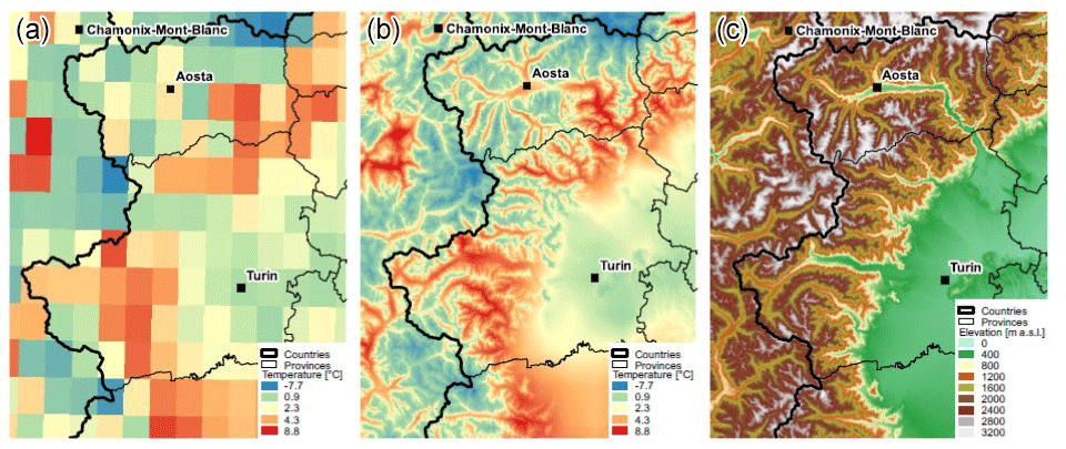
Figure 2Maximum temperature field at (a) 0.125∘ longitude–latitude spatial resolution from the original OI dataset and at (b) 250 m resolution after interpolation with orographic correction, for 1 January 2009. Panel (c) shows the orography of the study area from a digital elevation model derived from the SRTM project, interpolated at 250 m of spatial resolution.
3.2 Input data of the soil water model
The soil hydraulic properties have been estimated via pedotransfer functions (PTF) following Schaap et al. (2001) from the sand, clay and silt percentages taken from the soil map of the Piemonte Region (scale 1:250 000, IPLA, 2007). Computing the wilting point (WP) and field capacity (FC) via PTF, the total available water (TAW) is calculated for each layer as follows:
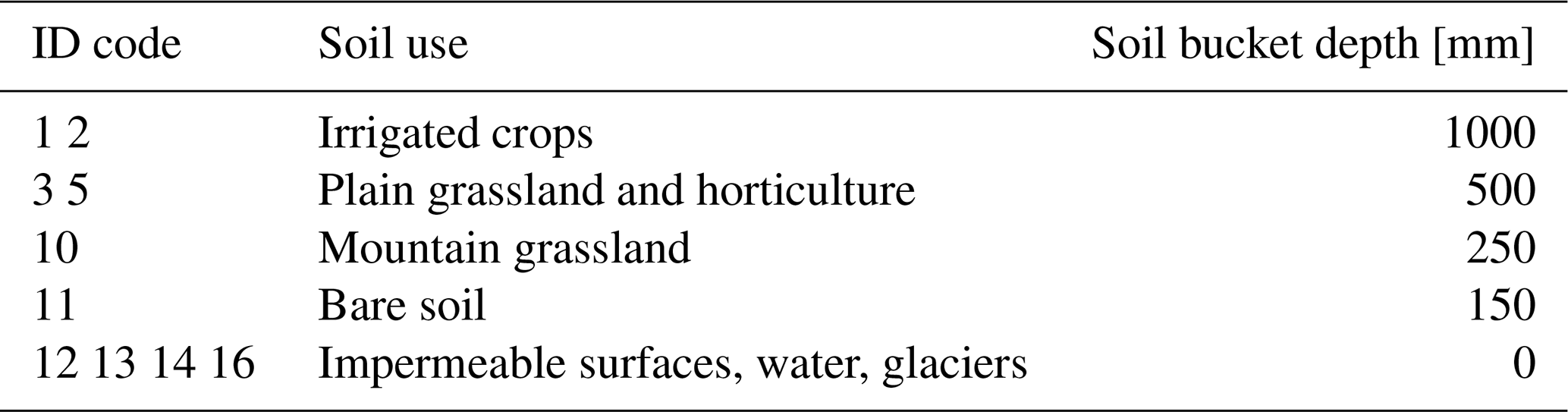
where r is the fraction of volume occupied by stones, and Ld is the layer depth, which is obtained by dividing the root zone depth z by the number of layers (seven; see Sect. 2.3). The root zone depth has been obtained using the land cover classes from the BDTRE database (Regione Piemonte, 2018a), listed in Table 2, converted into root zone depth using different root zone depths for each class, as listed in Table 3. The resulting root zone depth was compared with the soil depth provided by the soil map of the Piemonte Region (IPLA, 2007), choosing the minimum between the two depths. For trees, the water from the whole soil depth can be depleted, and so soil depth has been used. Because of the high spatial resolution of BDTRE, the raster has been produced with a 5 m × 5 m grid then resampled at 250 m by the mode criterion. Homogenizing data as a function of the evapotranspiration behaviour of each class, the different land cover classes have been aggregated (Table 2).

Table 3Soil bucket depth as a function of land cover class. For trees (codes 4, 6, 7, 8 and 9) the full soil depth from the soil map of the Piemonte Region is used.
Finally, considering that irrigation (here considered as water input) significantly modifies actual evapotranspiration, for quantifying the actually irrigated fields, we used the regional irrigation information system (Regione Piemonte, 2016), the agricultural crop survey and the historical maps within the actually utilized agricultural areas survey database (Regione Piemonte, 2006), for the years 2013, 2014 and 2015. The actual quantity of irrigation water and the number of irrigations have been evaluated using the measured data collected in experiments performed in real-world farms, both for surface irrigation (Canone et al., 2015) and for sprinklers (Canone et al., 2016).
Even if runoff was not considered in this study, following Kumar et al. (2016) it could be useful to quantify its variability with climate change. As suggested by Epting et al. (2021), this should be taken into account where river-fed aquifers are considered.
Reliable estimates of the hydrological response and of water availability in the coming decades generally require the implementation of a modelling chain consisting of global climate models (GCMs), which provide climate scenarios for the entire planet, regional climate models (RCMs) nested into global models providing lateral and boundary conditions for the regional simulation and, depending on the resolution which needs to be achieved, further downscaling procedures. At the end of the modelling chain, a hydrological model is thus forced with a high-resolution climatic input to simulate the hydrological response at the scale of interest. In this study, we used a small multi-member ensemble of the RCA4 RCM, (Strandberg et al., 2014) forced by five GCM simulations, able to provide the climatic variables of interest – surface air temperature and precipitation – at a spatial resolution of ∼12.5 km. More detailed analyses of the interplay between several GCMs and RCMs (Sorland et al., 2018) are outside of the operational water management scope of this paper. In this work we proceeded similarly to another recharge study (Allen et al., 2010) which used four GCMs and one RCM. They concluded that a range of GCMs should be considered for water management planning. The simulation outputs of this RCM from 1970 to 2050 have been analysed, considering two different emission scenarios for future projections among those defined by the IPCC (Intergovernmental Panel on Climate Change, IPCC, 2013; Moss et al., 2010), as described in Sect. 4.1. The model data were subsequently interpolated applying the same procedure employed for the OI observational dataset (see Sect. 3) and adjusted to correct the systematic bias which the model displays with respect to the OI reference climatology in a common time period (1986–2015; see Sect. 4.3 for a description of the post-processing procedure).
4.1 RCA4 regional climate model
In the following, we used model simulations of the RCA4 RCM (Strandberg et al., 2014) driven by five different GCMs, namely EC–Earth, CNRM–CM5, IPSL–CM5A–MR, HadGEM2–ES and MPI–ESM–LR, which provide lateral and boundary conditions for the regional simulation. Using one single RCM allowed us to obtain an ensemble of reasonably homogeneous simulations at the regional level but representing at the same time model uncertainties in future projections captured by the different large-scale GCMs. RCA4 is a state-of-the-art RCM which participated in CORDEX, the Coordinated Regional Climate Downscaling Experiment (http://wcrp-cordex.ipsl.jussieu.fr/, last access: 14 August 2020; Giorgi et al., 2009), sponsored by WCRP (World Climate Research Program), aimed at providing a global coordination of regional climate downscaling activities useful to support climate change adaptation policies. The simulations used in this study, in particular, are part of the EURO-CORDEX initiative (http://www.euro-cordex.net/, last access: 14 August 2020), which provides regional climate projections for Europe at two different spatial resolutions, ∼50 km (EUR-44, 0.44∘ resolution) and ∼12 km (EUR-11, 0.11∘ resolution). EURO-CORDEX includes a total of seven RCMs nested into several GCMs, whose simulations belong to the most recent Climate Model Intercomparison Project phase 5 (CMIP5 Taylor et al., 2012). The RCA4 model was chosen because, at the time of downloading the data from the CORDEX archive, it was the only RCM providing data at the finest available spatial resolution (∼12 km) and with sub-daily (3 h) temporal resolution (WCRP, 2009). For a detailed description of the RCA4 model and its validation, please refer to the technical report by Strandberg et al. (2014).
4.2 Emission scenarios
Future projections provided by climate models are based on a set of assumptions about the future evolution of the society in terms of energetic and technological choices, population growth, land use changes and others, which correspond to possible greenhouse gas emission and concentration pathways in the atmosphere. The fifth IPCC Assessment Report (IPCC, 2013) uses four different Representative Concentration Pathway (RCP) scenarios (Moss et al., 2010; van Vuuren et al., 2011) to evaluate how climate is likely to change by the end of the 21st century. For this study, two of these scenarios were considered, referred to as RCP4.5 and RCP8.5, as they were the only ones available for the model under consideration. RCP4.5 is a stabilization scenario in which emissions will be stabilized by 2070 and carbon dioxide concentrations in the atmosphere are expected to stabilize at about twice the pre-industrial level by the end of the century. RCP8.5 is an extreme business-as-usual scenario in which greenhouse gas emissions are not expected to stabilize and carbon dioxide concentrations will be more than tripled at the end of the century compared to pre-industrial levels.
4.3 RCM data post-processing
RCA4 simulation outputs were linearly interpolated on the UTM grid at 1 km resolution in the study area using the same method applied to the OI data and illustrated in Sect. 3. To avoid distortions and artefacts, the data were first mapped with the CDO tool (Climate Data Operators; v. 1.7) on a longitude–latitude grid at 0.001∘ resolution and then projected with GDALwarp (Geospatial Data Abstraction Library; v. 2.1) on the final UTM grid (WGS 84/UTM zone 32 N) at 1 km resolution. The intrinsic imperfections of climate model parameterizations and the errors in the model initialization are often reflected in an imperfect representation of the observed climate, which can give rise to biases. Model biases must be taken into account when the climate model outputs are used in impact studies, as impacts and feedbacks can be sensitive to the absolute values and the statistical properties of the climatic input. Bias correction methods are usually applied to correct the differences between climate model output and observed climatologies and are different depending on the variable and specific application which is considered (Hempel et al., 2013; Maraun, 2013; Maraun et al., 2010). In this study we used an additive correction factor for adjusting the temperature and a multiplicative correction factor for precipitation (a standard procedure for positive-defined fields) applied pixel by pixel and constant in time, in order to correct the differences in the long-term climatology calculated over a common time period between the simulated and observed fields. To this end, we calculated the long-term mean of the historical Euro-CORDEX simulations and of the OI dataset, already interpolated on the UTM grid, in the 30-year-long period from 1986 to 2015. In order to maintain the physical consistency between the minimum temperature and the maximum temperature, and thus avoid possible inversions, the same correction factor was used for daily minimum and maximum temperature data, calculated from the average between the daily minimum temperature and the maximum temperatures. The correction factor calculated to correct the model bias in the historical reference period was then applied to the future simulations. In addition to the bias adjustment, temperatures have been further corrected for the lapse rate, as already done for the OI data, based on Rolland (2003).
5.1 Trends in observed data
Historical data from 1959 to 2017 were analysed in each river catchment and sub-catchment, aggregating all data previously evaluated at the spatial resolution of 250 m, to find out significant trends both of the water balance terms and of the meteorological variables, for both the hydrological year and the quarterly analysis.
A linear regression was performed to calculate the temporal trends. The goodness-of-fit line was estimated with the coefficient of determination R2, and its statistical significance was evaluated considering the p value at a 5 % level (i.e. 95 % significance) (Wilks, 2011).
5.1.1 Hydrological year analysis
During the hydrological year, an almost complete snow melting usually occurs in the considered area. Thus, in Eq. (1) Pq refers to the whole precipitation amount and Pq−AET to drainage. Figure 3 shows the time series from 1959 to 2017 of the daily maximum temperature (in Kelvin, panel a), Pq (mm yr−1, panel b), AET (mm yr−1, panel c), and drainage (mm yr−1, panel d), for the Dora Riparia station in Turin as an example. It represents the driest watershed in this study, located in the middle of the study area with a west–east orientation (Fig. 1). In the Alps, this kind of valley is often characterized by foehn wind, corresponding to dry weather. Other examples in the Alps are Valais, Valle d'Aosta, Valtellina and Val Venosta.
Figure 3 reveals that, for this catchment, the daily maximum temperature has increased during the study period, with a statistically significant trend, as in all other catchments. The total precipitation, Pq, has decreased (p=0.059), while AET has increased (p=0.054), and drainage has significantly decreased (p=0.032). The catchment considered here is in the driest part of the study region, which is also the part where most of the significant trends of precipitation and AET were detected in the data analysis. The same approach is adopted for all the catchments in the study area. The results are summarized in Table S1 of the Supplement. For all catchments, hydrological year trends in maximum temperature are positive and statistically significant, ranging between 0.032 and 0.078 K yr−1. AET trends are also positive for all catchments and statistically significant in 14 out of 23 cases. In 13 cases out of 14, they were either in the western mountain Dora Riparia area or in the southern irrigated area. The finding of an increase in AET is not obvious. Pangle et al. (2014) found a decreasing trend of AET looking at data from a mesocosm experiment. Their results highlight that the hydrological response to climate warming can be attenuated where precipitation is out of phase with the vegetation growing season. Our results refer instead to an area where precipitation and growing season are not markedly out of phase. This can be due to the presence of the irrigated fields in the southern plains, where AET is mostly water-limited and to the forested areas in the western mountain part of the region, where AET is mostly energy-limited. Blyth et al. (2018) also found an increase in evapotranspiration under similar conditions, using a land surface model in Great Britain from 1961 to 2015. In a more theoretical work, Fatichi and Ivanov (2014) found AET to be quite unaffected by the imposed climate fluctuations, using the input data from four very different sites. This confirms the large role of spatial variability in the response of water balance to climate change.
The map in Fig. 4 represents the spatial distribution of annual actual evapotranspiration. It clearly shows the higher values of AET in the southern part of the region, where the irrigated fields play a major role, highlighting the importance of correctly modelling irrigation, as in the irrigation module implemented in our soil water model. The surface energy budget is heavily influenced by agricultural water management, and, together with air temperature increase, this leads to higher evapotranspiration average fluxes in comparison to non-irrigated crops.
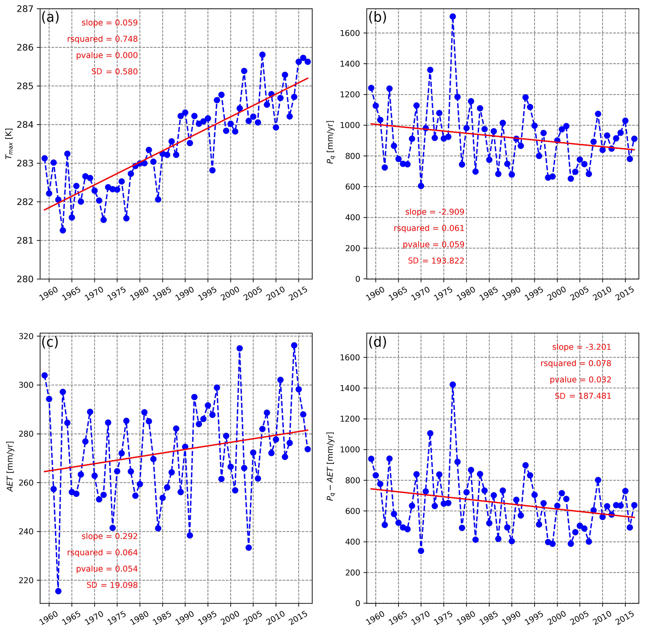
Figure 3Hydrological year time series of Tmax (a), Pq (b), AET (c) and drainage (d) along with their trends, R2, p values and standard deviations, for the time period from 1959 to 2017, at the Turin cross-section 66 (the location is shown in Fig. 1) of Dora Riparia river basin (average at the catchment level). The standard deviation, evaluated considering the detrended time series, provides a quantification of interannual variability.

Figure 4Spatial distribution of annual actual evapotranspiration.
Most catchments exhibit negative precipitation (Pq) trends, but only five cases display statistically significant trends. Precipitation at all catchments exhibits a high interannual variability (a quantification of interannual variability can be provided by the standard deviation, evaluated considering the detrended time series, shown in Table S1 of the Supplement), in accordance with the results of previous studies in the same area (Pavan et al., 2019; Baiamonte et al., 2019; Ciccarelli et al., 2008). A recent study has shown a low-frequency variability in the same historical years of this study for the Alpine region (Haslinger et al., 2021).
Drainage shows negative but mostly non-significant trends in all catchments. The seven catchments with significant decreasing trends all belong to the western and driest part of the region (Dora Riparia catchment). Four of them have significant trends both in Pq and AET, two of them have significant trends only in AET and one has significant trends only in Pq.
This area is characterized by much lower yearly total precipitation values than the northern one. Long-term climatological values of cumulative yearly precipitation in the western Dora Riparia area are Oulx, 552 mm; Susa, 710 mm; Beaulard, 680 mm; Bardonecchia, 724 mm; and Pragelato, 818 mm; while in the northern and wetter part they are Pont Canavese, 1228 mm; Viu, 1338 mm; and Germagnano, 1342 mm. The southern part is instead characterized by the following values: Cumiana, 924 mm, and Moncalieri, 882 mm.
To summarize, a slight negative trend is observed for precipitation and drainage over the last 60 years, showing a high spatial and interannual variability, as highlighted by the existing literature (Blöschl et al., 2019; Gudmundsson et al., 2017; Libertino et al., 2019). In Fig. 3, the values for the whole Dora Riparia catchment down to Turin are shown. This western part of the study area can be identified as the driest one, as already observed in a recent work by Blöschl et al. (2019), where decreasing precipitation trends combine with increasing evapotranspiration trends. This can be attributed to non-water-limited mountain vegetation in combination with increasing temperatures. Finally, the increasing evapotranspiration trends that characterize the southern part of the study area (due to irrigation by farmers) are not associated with significant decreasing precipitation trends, leading to a non-significant drainage variation over time, even if AET has relatively high values in the southern area (Fig. 4). Thus, in regions such as the one considered in this paper, when focusing on trend analysis, precipitation plays a major role in affecting drainage tendencies.
5.1.2 Analysis at the quarterly scale
The meteorological and hydrological variables at the quarterly timescale provide information on intra-annual variations. Figure 5 shows the trend results (colour code) for all catchments (identified by their ID number in the y axis of each panel) and for Tmax (panel a), rainfall plus snowmelt (panel b), AET (panel c) and drainage (panel d) from 1959 to 2017. The numerical value of the trend is displayed in a cell when it is statistically significant (p<0.05). When quarters are considered for the analysis, total precipitation (water input) is defined as the sum of liquid precipitation Pr and snowmelt Nf (see Sect. 2.3).

Figure 5Trend slope of all quarters and catchments considered. (a) Tmax, (b) precipitation, (c) AET and (d) drainage. Trend slope is specified if significant at a 5 % level. When quarters are considered, the precipitation is represented by the sum of liquid precipitation Pr and melted snow Nf.
Tmax shows positive and statistically significant trends in all catchments and quarters in the period 1959–2017, with values between 0.022 and 0.086 K yr−1. The increase in the daily maximum temperature is more evident in winter (first quarter) and autumn (fourth quarter). The time series of actual evapotranspiration show positive and significant trends in the majority of catchments and quarters, indicating an overall increase of AET in the entire study area. AET has a greater increase in the summer quarter (JAS). Positive trends in the first quarter are consistent with those observed for Tmax, both suggesting a possible anticipation of the growing season.
While historical yearly precipitation trends are overall negative, the quarterly analysis shows a significant decrease of precipitation in the first and second quarters, confirming that precipitation trends in north-western Italy depend on the considered temporal aggregation (Brunetti et al., 2006). The drainage trend analysis shows an overall reduction in the first and second quarters, with larger decreases in AMJ, but significant only for six watersheds, again in the western driest part of the region. The third and fourth quarters show slight positive non-significant trends.
A visual comparison between yearly and quarterly analysis is shown in Fig. 6, where precipitation (panel a) and drainage (panel b) trends are displayed over the whole study area. This figure clearly shows again the spatial pattern of hydrological changes, with negative trends in both precipitation plus snowmelt and discharge in spring. The dry western area is mainly represented by the Dora Riparia valley. Beside the spatial issue, the quarterly results show the importance of the time variability of precipitation. It confirms the importance of the computation at the daily scale (Healy, 2010). Masbruch et al. (2016) have also shown the sensitivity of drainage to rainfall time variability, and Fatichi and Ivanov (2014) stressed the importance of short periods (order of hours or days) with high AET.
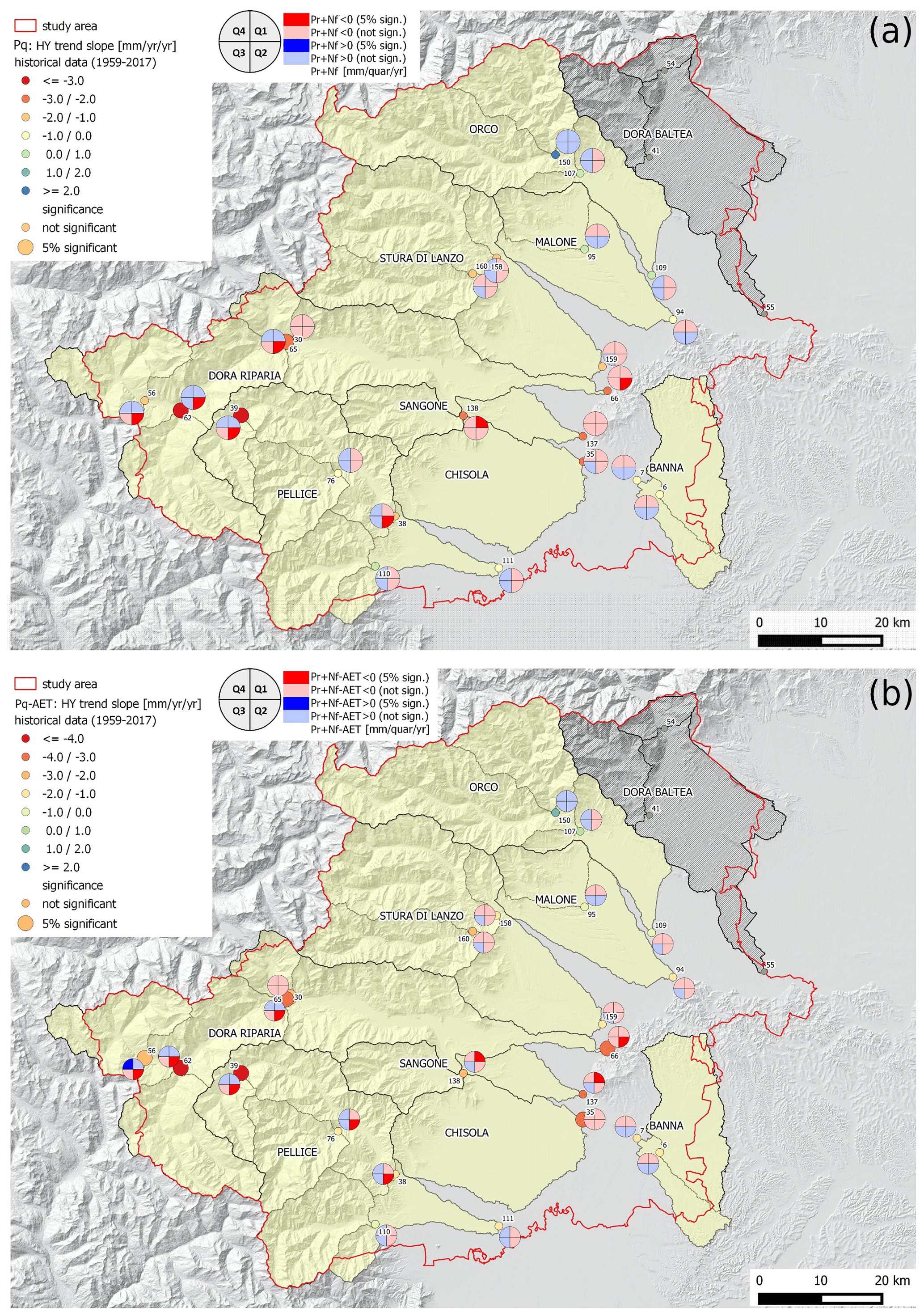
Figure 6Trend slope at the catchment level for all studied catchments. (a) Total precipitation and (b) drainage. Hydrological year (full dots) and quarterly trend values (four-segments circles) are jointly represented, and trend significance is also indicated. When quarters are considered, the precipitation is the sum of liquid precipitation Pr and melted snow Nf. Topographic shading is based on DEM data from the Risknat project – “Base topografica transfrontaliera, ARPA Piemonte” (http://webgis.arpa.piemonte.it/ags101free/rest/services/topografia_dati_di_base/Sfumo_Europa_WM/MapServer, last access: 14 August 2020).
5.2 Mid-century projections of drainage
This section reports the results for the future projections of drainage. As already mentioned, this variable allows us to quantify the groundwater resource availability using only meteorological variables provided by the climate models. The simulations have been performed up to 2050 using the ensemble of simulations obtained with the RCM described in Sect. 4.1, at both hydrological year and quarterly scales.
5.2.1 Hydrological year analysis
Table S2 of the Supplement shows the drainage trend slopes from 2018 up to 2050 for each catchment in the study area using climate projections under the RCP4.5 and the RCP8.5 scenarios. Drainage trends in the RCP4.5 scenario are often negative but not statistically significant. These negative trends become stronger and occasionally statistically significant in the more extreme RCP8.5 scenario.
As a general statement, also taking into account the variability within the projection ensemble, the rather small values of drainage trends and their limited significance do not suggest a strong variation from a steady-state yearly drainage condition until 2050, with total precipitation that shows a slight decrease. We find a slight drainage increase with higher precipitation amounts, decreasing trends with higher daily maximum temperature and, above all, a strong interannual variability (see, as an example, the standard deviation evaluated for the detrended time series shown in Fig. 7).
The projections of Pq−AET (drainage) for two different cross-sections of the study area, the Dora Riparia station in Turin (catchment ID 66) and the Orco station in S. Benigno (catchment ID 109), are shown in Fig. 7. These two cases were shown because the two catchments are among the largest ones (as shown in Table S1 of the Supplement, 1243 and 829 km2, respectively), and they represent, respectively, the drier (western) and the wetter (northern) parts of the region.
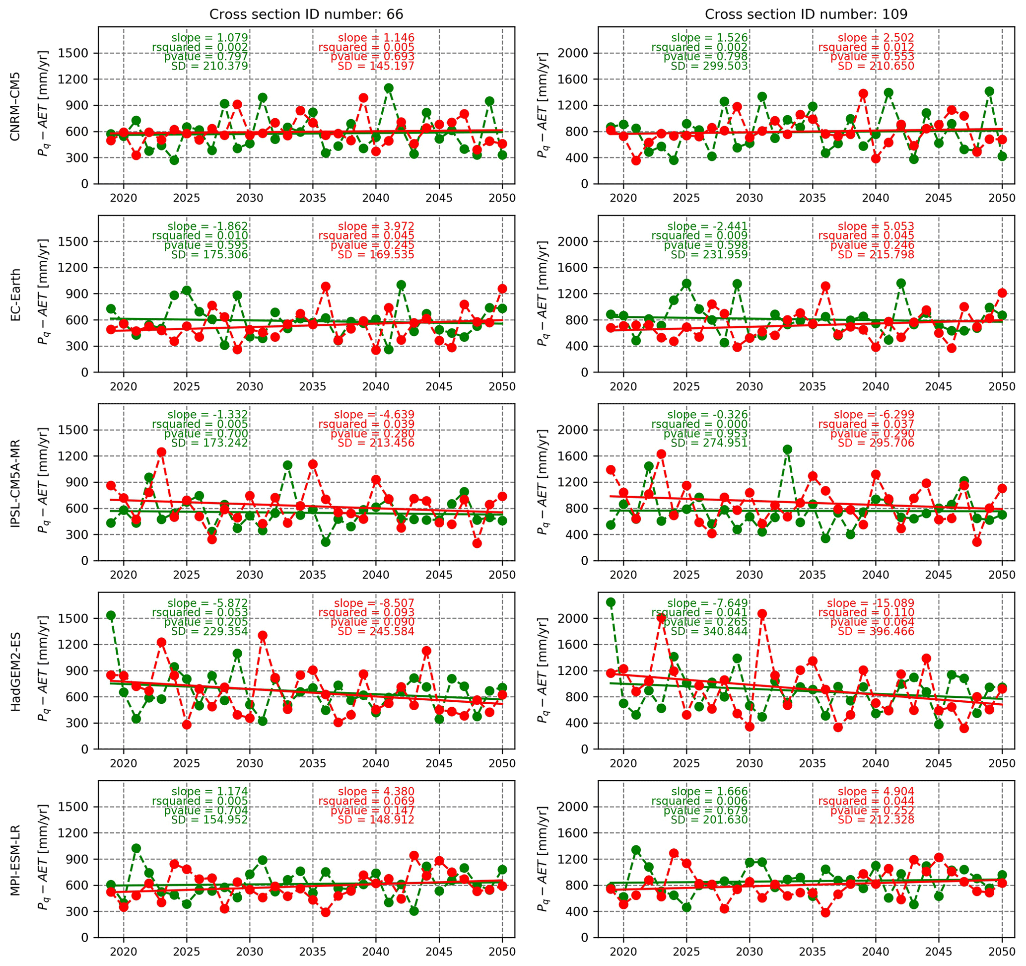
Figure 7Yearly drainage projections (RCP4.5 scenario in green and RCP8.5 scenario in red) for two different cross-sections (Dora Riparia in Torino, cross-section 66, and Orco in San Benigno, cross-section 109) of the studied area. Each row corresponds to the results obtained with one GCM driving the RCA4 RCM. The slope of the regression line, the coefficient of determination R2, the p value and the standard deviation evaluated for the detrended time series are also indicated.
The overall results at yearly timescale can be summarized as follows:
-
Tmax shows positive trends that are almost always significant for all model realizations and both scenarios.
-
Pq has either positive or negative trends (according to the different GCMs and scenarios), rarely significant. In particular, RCA4 driven by the CNRM-CM5 and MPI–ESM–LR models shows positive trends for all catchments and scenarios. RCA4 driven by EC-Earth shows negative trends in all catchments when the RCP4.5 scenario is considered and positive trends for the RCP8.5 scenario. Finally, RCA4 driven by IPSL–CM5A–MR and HadGEM2–ES shows negative trends in the whole study area for both the RCP4.5 and RCP8.5 scenarios.
-
AET has either positive and negative trends, rarely significant. In detail, considering the RCP4.5 scenario, RCA4 driven by the HadGEM2–ES and MPI–ESM–LR models shows positive trends in the whole study area; when driven by EC-Earth and IPSL–CM5A–MR it shows negative trends in almost all catchments, and when driven by CNRM-CM5, it shows spatial heterogeneity (only Malone, Sangone, Chisola and Orco primary catchments have positive trends). Considering the RCP8.5 scenario, RCA4 driven by CNRM-CM5, EC-Earth and MPI–ESM–LR shows positive trends in the whole study area that are almost always significant for the case of the CNRM-CM5 model. RCA4 driven by IPSL–CM5A–MR has negative trends for all catchments, while RCA4 driven by HadGEM2–ES shows negative trends only in Banna, Chisola, Malone and Sangone primary catchments.
-
There are slight positive drainage trends with higher precipitation amounts, negative trends with higher Tmax and high interannual variability.
To summarize, we observe a large variability between the different projections, as also found in Crosbie et al. (2013) and in Persaud et al. (2020), with a much less clear pattern in spatial variability if compared with the historical data trend evaluations.
5.2.2 Quarterly analysis
Projections of drainage evaluated at the seasonal timescale show again a large variability within the ensemble of projections. However, a general tendency to drainage increase in the first quarter and to drainage decrease in the third and fourth quarters, JAS and OND, emerges. Tables S3–S6 of the Supplement show the drainage trend (expressed in mm per quarter per year) in the four quarters.
In the first quarter (JFM), the models mostly agree in their indication of a drainage increase up to 2050 over the whole study area, with a wider agreement for RCP4.5 (four out of five models concur in all catchments). In the second quarter (AMJ), in all river basins, at least three out of five models estimate a drainage decrease for the RCP8.5 scenario, not for RCP4.5. In the third (three out of five models) and fourth (four out of five models) quarters, an overall tendency of drainage decrease in the whole study area for RCP4.5 is evident.
For the other meteoclimatic and water balance variables, at quarterly timescale we can report the following:
-
Tmax shows positive trends in all quarters, almost always significant for all models and scenarios.
-
In all quarters, both rainfall plus snowmelt Pq and rainfall (Pr) have both positive and negative trends, rarely significant. Rainfall has almost everywhere a weak positive trend in the first quarter, rarely significant. Snowfall shows broad negative trends, almost always significant.
-
AET shows broad positive trends in the first and second quarters, despite some differences between the models. In the third quarter, an overall decreasing tendency can be observed, while in the fourth quarter, trend slopes have values close to zero.
Stoll et al. (2011) also found a major role of the time variability of precipitation in recharge projections for a catchment in northern Switzerland. Konapala et al. (2020) indicate changes in long-term drainage, but they recall the limitations in the ability of current generation coupled climate models to capture the key drivers of persistent weather extremes.
Assessing the impacts of climate change on groundwater resources represents a priority in water management, besides being an important scientific challenge. In this framework, a proactive engagement of stakeholders is still lacking to a large part, and stakeholders are mainly considered to be final users who download pre-computed decision-relevant scientific information in order to develop and apply adaptation or mitigation strategies. In this study a stakeholder-driven research study was carried out to quantify the role of groundwater in an area providing water to about 2.3 million people. This area is characterized by a very large spatial variability of precipitation, due to the proximity of high mountains and of the sea.
This work quantifies the trends of precipitation, temperature and actual evapotranspiration in order to estimate the trend of drainage as a proxy for the water available for drinking purposes. The analyses have been performed both at the hydrological year and at the quarterly timescales. We analysed past and future conditions, using a historical climate dataset providing minimum and maximum daily air temperature and precipitation data for the period 1959–2017 and future projections from a multi-member ensemble of a regional climate model up to 2050, in order to be compliant with the time frame of water management objectives.
As suggested by Taylor et al. (2013), the role of irrigated agriculture is considered. In such a context, irrigation, that significantly contributes to the increase of actual evapotranspiration as a consequence of the air temperature increase, was simulated in a novel way. More specifically, the results of field studies with both surface and sprinkler irrigation methods were used, combining them with crop and irrigation regional databases. AET has its greatest increase in summer, while in the first 3 months of the year, there is a consistent increase of both Tmax and AET, suggesting a possible anticipation of the growing season. Regarding drainage, our analysis revealed a very strong interannual variability in the historical period, as well as remarkable spatial differences, i.e. across the different catchments. It was found that the driest part of the region (the Dora Riparia valley) shows significant negative precipitation and drainage trends, both yearly and from January to June, confirming the seasonal variations found by Epting et al. (2021) and giving interesting hints for other dry climate valleys in the Alps. The increasing trend of yearly actual evapotranspiration is positive for all catchments and statistically significant in 14 out of 23 cases, namely both in the Dora Riparia valley and in the southern irrigated area. This quantity, together with the relevant interannual variability of precipitation, has to be monitored in the future for its potential effects on drainage. Interestingly, only the Dora Riparia valley and the most western part of Pellice catchment (cross-section 39) show significant negative trends for drainage, combining a significant decrease of precipitation and increase of AET due to mountain non-water-limited vegetation. The significant increasing trend of AET due to irrigation of the southern irrigated plain area led to a non-significant drainage because it was not combined with a significant decreasing of precipitation.
As for the future projections, there is a large inter-model variability, as in Crosbie et al. (2013) and in Persaud et al. (2020), of all hydrological variables, which is evident for all catchments, and almost no significant trends are present. This last result is in line with Gudmundsson et al. (2017) for this part of Europe. Also interestingly, the future scenarios do not reproduce the spatial variability of the historical analyses, although the soil and irrigation model used was the same.
This study constitutes a knowledge basis which aids a better informed management, infrastructural and supply decisions in the considered study area, with a methodology that could also be applied in other areas in the world. In the Dora Riparia area, a new drinking water aqueduct (70 km long, 800 L s−1 discharge and EUR 130 million cost) has been built to provide water from an existing hydroelectric reservoir at 1600 m a.s.l., close to the border with France, down to Turin (Società Metropolitana Acque Torino, 2019). It will allow continued pumping from the Dora Riparia aquifer to be avoided, which has a negative trend of drainage and has so far provided drinking water to 27 municipalities. A complementary hydraulic research study has been performed by the Polytechnic of Turin (Fellini et al., 2018). The characteristics of spatial and temporal variability of aquifer recharge found in this paper will be of interest for other European areas, particularly in the Mediterranean area and in the Alps, where multiple anthropogenic pressures act on groundwater resources and where climate change will exacerbate competition between different users. Finally, climate-change-related spatial variability of precipitation has been similarly shown in a recent work about European floods for the period 1960–2010 (Blöschl et al., 2019). Even if that is a larger scale study, it is possible to see a decreasing trend for Dora Riparia, to be compared to a slightly increasing trend for the rest of northern Italy, a behaviour similar to the one found in this work. The outcomes of this paper reinforce the findings of two different precipitation regimes over Europe, the Mediterranean and the continental one. Both can be found in our study area, and the Dora Riparia valley seems to be the bridge between them.
In this research, climate scientists, hydrologists, agricultural and soil scientists worked together with the experts from the local water utility to assess the water potential of the study area and better understand the role of groundwater in the future provision of water to the community. The approach followed is tailored to stakeholder needs, and the outcomes of the study are intended to drive or support local policies, in a general context which stimulated and supported participatory planning, driven by state-of-the art climate information and projections. Our results will be integrated in the definition and refinement of the study-area long-term guidelines and strategic development for groundwater resources protection and infrastructural provision and planning. It will be a part of a wider effort to strengthen good water resource management and governance.
The derived datasets presented in this study can be obtained upon request to the corresponding author. Post-processed data are reproducible following the detailed descriptions of Sects. 2 and 3 and are available upon request to the authors. All other datasets cited in the text can be retrieved following the instructions in the relevant citations. In particular: The ARPA Piemonte NWIOI dataset is available at http://www.arpa.piemonte.it/rischinaturali/tematismi/clima/confronti-storici/dati/dati.html (ARPA Piemonte, 2010a); the SRTM 90 m DEM Digital Elevation Database is available at http://srtm.csi.cgiar.org (Jarvis et al., 2008); the Regione Piemonte Anagrafe agricola – data warehouse is available at: https://servizi.regione.piemonte.it/catalogo/anagrafe-agricola-data-warehouse (Regione Piemonte, 2006); the Regione Piemonte Bonifica e Irrigazione (SIBI) is available at https://www.regione.piemonte.it/web/temi/agricoltura/agroambiente-meteo-suoli/bonifica-irrigazione-sibi (Regione Piemonte, 2016); the Regione Piemonte BDTRE is available at https://www.geoportale.piemonte.it/geonetwork/srv/ita/catalog.search#/metadata/r_piemon:94379297-e72a-41f8-918d-f497a956eb39 (Regione Piemonte, 2018a).
The supplement related to this article is available online at: https://doi.org/10.5194/hess-26-407-2022-supplement.
All the authors conceived the study. EP and JvH provided and preprocessed the meteoclimatic data. GM, GV, MP, DC, DG, IB and SF performed and analysed the hydrological simulations and prepared some of the figures. EB and SF analysed the results. EB and IB prepared the figures and EB all the tables. EB, EP, JvH, AP and SF wrote the paper with support from all the authors.
The contact author has declared that neither they nor their co-authors have any competing interests.
Publisher's note: Copernicus Publications remains neutral with regard to jurisdictional claims in published maps and institutional affiliations.
The authors would like to thank the Risk Responsible Resilience Interdepartmental Centre (R3C) DIST–PoliTO for valuable collaboration and ARPA Piemonte for kind support.
This work has been funded by Società Metropolitana Acque Torino S.p.A. Research has been supported in part by “Dipartimento di Eccellenza” DIST department funds and “PRIN MIUR 2017SL7ABC_005 WATZON Project” and by the Project of National Interest NextData of the MIUR (Italian Ministry for Education, University and Research).
This paper was edited by Günter Blöschl and reviewed by two anonymous referees.
Agnese, C., Baiamonte, G., Cammalleri, C., Cat Berro, D., Ferraris, S., and Mercalli, L.: Statistical analysis of inter-arrival times of rainfall events for Italian Sub-Alpine and Mediterranean areas, Adv. Sci. Res., 8, 171–177, https://doi.org/10.5194/asr-8-171-2012, 2012. a
Aguilar, C., Herrero, J., and Polo, M. J.: Topographic effects on solar radiation distribution in mountainous watersheds and their influence on reference evapotranspiration estimates at watershed scale, Hydrol. Earth Syst. Sci., 14, 2479–2494, https://doi.org/10.5194/hess-14-2479-2010, 2010. a
Allen, D., Cannon, A., Toews, M., and Scibek, J. Variability in simulated recharge using different GCMs, Water Resour. Res., 46, https://doi.org/10.1029/2009WR008932, 2010. a
Allen, R., Pereira, L., Raes, D., and Smith, M.: FAO irrigation and drainage paper No. 56, Food and Agriculture Organization of the United Nations, Tech. Rep. 56, 1998. a, b, c
ARPA Piemonte: NWIOI daily data, Version 2.1, data updated daily, Rischi Naturali Archive Center [data set], available at: http://www.arpa.piemonte.it/rischinaturali/tematismi/clima/confronti-storici/dati/dati.html (last access: 14 August 2020), 2010a. a, b
ARPA Piemonte: Metodologia dell'Optimal Interpolation, Tech. rep., Arpa Piemonte, Dipartimento Sistemi Previsionali, available at: http://rsaonline.arpa.piemonte.it/meteoclima50/pdf/metodologia.pdf (last access: 14 August 2020), 2010b. a
Baiamonte, G., Mercalli, L., Cat-Berro, D., Agnese, C., and Ferraris, S.: Modelling the frequency distribution of interarrival times from daily precipitation time-series in North-West Italy, Hydrol. Res., 50, 339–357, https://doi.org/10.2166/nh.2018.042, 2019. a, b, c
Bastiancich, L., Lasagna, M., Mancini, S., Falco, M., and Luca, D. A. D.: Temperature and discharge variations in natural mineral water springs due to climate variability: a case study in the Piedmont Alps (NW Italy), Environ. Geochem. Health, 1-24, https://doi.org/10.1007/s10653-021-00864-8, 2021. a
Baudena, M., Bevilacqua, I., Canone, D., Ferraris, S., Previati, M., and Provenzale, A.: Soil water dynamics at a midlatitude test site: Field measurements and box modeling approaches, J. Hydrol., 414–415, 329–340, https://doi.org/10.1016/j.jhydrol.2011.11.009, 2012. a
Bertrand, G., Siergieiev, D., Ala-Aho, P., and Rossi, P.: Environmental tracers and indicators bringing together groundwater, surface water and groundwater-dependent ecosystems: importance of scale in choosing relevant tools, Environ. Earth Sci., 72, 813–827, https://doi.org/10.1007/s12665-013-3005-8, 2014. a
Blöschl, G., Hall, J., Viglione, A., Perdigão, R. A. P., Parajka, J., Merz, B., Lun, D., Arheimer, B., Aronica, G. T., Bilibashi, A., Boháč, M., Bonacci, O., Borga, M., Čanjevac, I., Castellarin, A., Chirico, G. B., Claps, P., Frolova, N., Ganora, D., Gorbachova, L., Gül, A., Hannaford, J., Harrigan, S., Kireeva, M., Kiss, A., Kjeldsen, T. R., Kohnová, S., Koskela, J. J., Ledvinka, O., Macdonald, N., Mavrova-Guirguinova, M., Mediero, L., Merz, R., Molnar, P., Montanari, A., Murphy, C., Osuch, M., Ovcharuk, V., Radevski, I., Salinas, J. L., Sauquet, E., Šraj, M., Szolgay, J., Volpi, E., Wilson, D., Zaimi, K., and Živković, N.: Changing climate both increases and decreases European river floods, Nature, 573, 108–111, https://doi.org/10.1038/s41586-019-1495-6, 2019. a, b, c, d
Blyth, E. M., Martinez-de la Torre, A., and Robinson, E. L.: Trends in evapotranspiration and its drivers in Great Britain: 1961 to 2015, Hydrol. Earth Syst. Sci. Discuss. [preprint], https://doi.org/10.5194/hess-2018-153, 2018. a
Brunetti, M., Maugeri, M., Nanni, T., Auer, I., Bohm, R., and Schoner, W.: Precipitation variability and changes in the greater Alpine region over the 1800-2003 period, J. Geophys. Res.-Atmos., 111, D11107, https://doi.org/10.1029/2005JD006674, 2006. a
Canone, D., Previati, M., Bevilacqua, I., Salvai, L., and Ferraris, S.: Field measurements based model for surface irrigation efficiency assessment, Agric. Water Manage., 156, 30–42, 2015. a, b
Canone, D., Previati, M., and Ferraris, S.: Evaluation of stem-flow effects on the spatial distribution of soil moisture using TDR monitoring and an infiltration model, Asce J. Irrig. Drain. Eng., 143, 04016075–1–04016075–14, https://doi.org/10.1061/(ASCE)IR.1943-4774.0001120, 2016. a, b
CH2018 Project Team: CH2018 – Climate Scenarios for Switzerland, Technical Report, National Centre for Climate Services, Zurich, ISBN 978-3-9525031-4-0, 2018. a
Ciccarelli, N., von Hardenberg, J., Provenzale, A., Ronchi, C., Vargiu, A., and Pelosini, R.: Climate variability in north-western Italy during the second half of the 20th century, Global Planet. Change, 63, 185–195, https://doi.org/10.1016/j.gloplacha.2008.03.006, 2008. a, b
Condon, L., Atchley, A., and Maxwell, R.: Evapotranspiration depletes groundwater under warming over the contiguous United States, Nat. Commun., 11, 873, 1–8, https://doi.org/10.1038/s41467-020-14688-0, 2020. a, b
Confortola, G., Soncini, A., and Bocchiola, D.: Climate change will affect hydrological regimes in the Alps, J. Alp. Res., 101-3, https://doi.org/10.4000/rga.2176, 2013. a
Crosbie, R., Scanlon, B., Mpelasoka, F., Reedy, R., and Gates, J.: Potential climate change effects on groundwater recharge in the High Plains Aquifer, USA, Water Resour. Res., 49, 3936–3951, https://doi.org/10.1002/wrcr.20292, 2013. a, b, c
De Luca, D., Lasagna, M., and Debernardi, L.: Hydrogeology of the western Po plain (Piedmont, NW Italy), J. Maps, 16, 265–273, https://doi.org/10.1080/17445647.2020.1738280, 2020. a, b
Desiato, F., Fioravanti, G., Fraschetti, P., Perconti, W., and Piervitali, E.: Il clima futuro in Italia: analisi delle proiezioni dei modelli regionali. Stato dell'Ambiente 58/2015, ISPRA, Tech. rep., 2015. a
DeWalle, D. and Rango, A.: Principles of snow hydrology, Cambridge Univ. Press, Cambridge, UK, 2008. a
Doveri, M., Menichini, M., and Scozzari, A.: Protection of groundwater resources: worldwide regulations, scientific approaches and case study, Springer, Berlin, DEU, 40, 13–30, https://doi.org/10.1007/698_2015_421, 2016. a
Epting, J., Huggenberger, P., Radny, D., Hammes, F., Hollender, J., Page, R. M., Weber, S., Bänninger, D., and Auckenthaler, A.: Spatiotemporal scales of river-groundwater interaction – The role of local interaction processes and regional groundwater regimes, Sci Total Environ., 618, 1224–1243, https://doi.org/10.1016/j.scitotenv.2017.09.219, 2018. a, b
Epting, J., Michel, A., Affolter, A., and Huggenberger, P.: Climate change effects on groundwater recharge and temperatures in Swiss alluvial aquifers, J. Hydrol., 11, 100071, https://doi.org/10.1016/j.hydroa.2020.100071, 2021. a, b, c, d, e, f
Fatichi, S. and Ivanov, V.: Interannual variability of evapotranspiration and vegetation productivity, Water Resour. Res., 50, 3275–3294, https://doi.org/10.1002/2013WR015044, 2014. a, b
Fellini, S., Vesipa, R., Boano, F., and Ridolfi, L.: Multipurpose Design of the Flow-Control System of a Steep Water Main, J. Water Resour. Plan. Manag. ASCE, 144, 05017018-1, https://doi.org/10.1061/(ASCE)WR.1943-5452.0000867, 2018. a
Giorgi, F., Jones, C., and Asrar, G.: Addressing climate information needs at the regional level: the CORDEX framework, World Meteorological Organization (WMO) Bulletin, 58, 175, 2009. a
Gudmundsson, L., Seneviratne, S., and Zhang, X.: Anthropogenic climate change detected in European renewable freshwater resources, Nat. Climate Change, 7, 813–817, https://doi.org/10.1038/NCLIMATE3416, 2017. a, b, c
Haslinger, K., Hofstatter, M., Schoener, W., and Bloeschl, G.: Changing summer precipitation variability in the Alpine region: on the role of scale dependent atmospheric drivers, Clim. Dynam., 57, 1009–1021, https://doi.org/10.1007/s00382-021-05753-5, 2021. a
Healy, R. W.: Estimating groundwater recharge, Cambridge, Cambridge, UK, 2010. a, b, c, d, e, f
Hempel, S., Frieler, K., Warszawski, L., Schewe, J., and Piontek, F.: A trend-preserving bias correction – the ISI-MIP approach, Earth Syst. Dynam., 4, 219–236, https://doi.org/10.5194/esd-4-219-2013, 2013. a
IPCC: Climate Change 2007: Impacts, Adaptation and Vulnerability. Contribution of Working Group II to the Fourth Assessment Report of the Intergovernmental Panel on Climate Change, edited by: Parry, M. L., Canziani, O. F., Palutikof, J. P., van der Linden, P. J., and Hanson, C. E., Cambridge University Press, Cambridge, UK, ISBN 978 0521 88010-7, 2007. a
IPCC: Climate Change 2013: The Physical Science Basis. Contribution of Working Group I to the Fifth Assessment Report of the Intergovernmental Panel on Climate Change, Cambridge University Press, Cambridge, United Kingdom and New York, NY, USA, https://doi.org/10.1017/CBO9781107415324, 2013. a, b
IPCC: Climate Change 2014: Synthesis Report. Contribution of Working Groups I, II, and III to the Fifth Assessment Report of the Intergovernmental Panel on Climate Change, IPCC, Geneva, Switzerland, 2014. a, b, c
IPLA: Carta dei suoli del Piemonte a scala 1:250 000, Tech. rep., IPLA, Regione Piemonte, Firenze, Italy, 2007. a, b
Jarvis, A., Guevara, E., Reuter, H., and Nelson, A.: Hole-filled SRTM for the globe: version 4: data grid, published by CGIAR-CSI on 19 August 2008, CGIAR-CSI SRTM 90m Database [data set], available at: (http://srtm.csi.cgiar.org, last access: 14 August 2020), 2008. a, b
Jiménez Cisneros, B., Oki, T., Arnell, N., Benito, G., Cogley, J., Doll, P., Jiang, T., and Mwakalila, S.: Freshwater resources, Cambridge University Press, 2014. a, b, c
Kalbus, E., Reinstorf, F., and Schirmer, M.: Measuring methods for groundwater – surface water interactions: a review, Hydrol. Earth Syst. Sci., 10, 873–887, https://doi.org/10.5194/hess-10-873-2006, 2006. a
Konapala, G., Mishra, A. K., Wada, Y., and Mann, M. E.: Climate change will affect global water availability through compounding changes in seasonal precipitation and evaporation, Nat. Commun., 11, 3044, https://doi.org/10.1038/s41467-020-16757-w, 2020. a, b
Kumar, S., Zwiers, F., Dirmeyer, P., Lawrence, D., Shresta, R., and Werner, A. T.: Terrestrial contribution to the heterogeneity in hydrological changes under global warming, Water Resour. Res., 52, 3127–3142, 2016. a
Lasagna, M., Luca, D. D., and Franchino, E.: Nitrate contamination of groundwater in the western Po Plain (Italy): the effects of groundwater and surface water interactions, Environ. Earth Sci., 75, 240, https://doi.org/10.1007/s12665-015-5039-6, 2016. a, b
Li, B., Rodell, M., and Famiglietti, J. S.: Groundwater variability across temporal and spatial scales in the central and northeastern U.S., J. Hydrol., 525, 769–780, https://doi.org/10.1016/j.jhydrol.2015.04.033, 2015. a
Libertino, A., Ganora, D., and Claps, P.: Evidence for increasing rainfall extremes remains elusive at large spatial scales: the case of Italy, Geophys. Res. Lett., 46, 7437–7446, https://doi.org/10.1029/2019GL083371, 2019. a, b
Maraun, D.: Bias correction, quantile mapping, and downscaling: revisiting the inflation issue, J. Climate, 26, 2137–2143, 2013. a
Maraun, D., Wetterhall, F., Ireson, A. M., Chandler, R. E., Kendon, E. J., Widmann, M., Brienen, S., Rust, H. W., Sauter, T., Themeßl, M., Chun, K. P., Goodess, C. M., Jones, R. G., Onof, C., Vrac, M., Thiele-Eich, I., and Thiele-Eich, I.: Precipitation downscaling under climate change: Recent developments to bridge the gap between dynamical models and the end user, Rev. Geophys., 48, RG3003, https://doi.org/10.1029/2009RG000314, 2010. a
Masbruch, M., Rumsey, C., Gangopadhyyay, S., Susong, D., and Pruitt, T.: Analyses of infrequent (quasi-decadal) large groundwater recharge events in the northern Great basin: their importance for groundwater availability, use, and management, Water Resour. Res., 52, 7819–7836, 2016. a, b
Moeck, C., Grech-Cumbo, N., Podgorski, J., Bretzler, A., and Gurdak, J.: A global-scale dataset of direct natural groundwater recharge rates: a review of variables, processes and relationships, Sci. Total Environ., 717, 1–19, https://doi.org/10.1016/j.scitotenv.2020.137042, 2020. a
Moench, M., Burke, J., and Moench, Y.: Rethinking the Approach to Groundwater and Food Security, Tech. Rep. Water Reports 24, Food and Agriculture Organization of the United Nations, Rome, Italy, 2003. a
Moss, R. H., Edmonds, J. A., Hibbard, K. A. , Manning, M. R., Rose, S. K., van Vuuren, D. P., Carter, T. R., Emori, S., Kainuma, M., Kram, T., Meehl, G. A., Mitchell, J. F. B., Nakicenovic, N., Riahi, K., Smith, S. J., Stouffer, R. J., Thomson, A. M., Weyant, J. P., and Wilbanks, T. J.: The next generation of scenarios for climate change research and assessment, Nature, 463, 747–756, https://doi.org/10.1038/nature08823, 2010. a, b
Pangle, L., Gregg, J., and McDonnell, J.: Rainfall seasonality and an ecohydrological feedback offset the potential impact of climate warming on evapotranspiration and groundwater recharge, Water Resour. Res., 50, 1308–1321, https://doi.org/10.1002/2012WR013253, 2014. a, b, c
Pavan, V., Antolini, G., Barbiero, R., Berni, N., Brunier, F., Cacciamani, C., Cagnati, A., Cazzuli, O., Cicogna, A., De Luigi, C., Di Carlo, E., Francioni, M., Maraldo, L., Marigo, G., Micheletti, S., Onorato, L., Panettieri, E., Pellegrini, U., Pelosini, R., Piccinini, D., Ratto, S., Ronchi, C., Rusca, L., Sofia, S., Stelluti, M., Tomozeiu, R., and Torrigiani Malaspina, T.: High resolution climate precipitation analysis for north-central Italy, 1961–2015, Clim. Dynam., 52, 3435–3453, https://doi.org/10.1007/s00382-018-4337-6, 2019. a
Persaud, E., Levison, J., MacRitchie, S., Berg, S., Parker, B., and Sudicky, E.: Integrated modelling to assess climate change impacts on groundwater and surface water in the Great lakes Basin using diverse climate forcing, J. Hydrol., 584, 1–15, https://doi.org/10.1016/j.jhydrol.2020.124682, 2020. a, b, c
Pradier, S., Chong, M., and Roux, F.: Radar observations and numerical modeling of a precipitation line during MAP IOP 5, Mon. Weather Rev., 130, 2533–2553, 2002. a
Raco, B., Vivaldo, G., Doveri, M., Menichini, M., Masetti, G., Battaglini, R., Irace, A., Fioraso, G., Marcelli, I., and Brussolo, E.: Geochemical, geostatistical and time series analysis techniques as a tool to achieve the Water Framework Directive goals: An example from Piedmont region (NW Italy), J. Geochem. Explor., 229, 106832, https://doi.org/10.1016/j.gexplo.2021.106832, 2021. a
Raffelli, G., Previati, M., Canone, D., Gisolo, D., Bevilacqua, I., Capello, G., Biddoccu, M., Cavallo, E., Deiana, R., Cassiani, G., and Ferraris, S.: Local- and Plot-Scale Measurements of Soil Moisture: Time and Spatially Resolved Field Techniques in Plain, Hill and Mountain Sites, Water, 9, 706, https://doi.org/10.3390/w9090706, 2017. a
Regione Piemonte: Anagrafe agricola del Piemonte, Regione Piemonte [data set], available at: http://www.sistemapiemonte.it/cms/privati/agricoltura/servizi/367-anagrafe-agricola-unica-data-warehouse (last access: 14 August 2020), 2006. a, b
Regione Piemonte: SIBI Sistema Informativo della Bonifica e Irrigazione, retrieved online from Regional Irrigation Information System Archive Center, Regione Piemonte [data set], available at: https://www.regione.piemonte.it/web/temi/agricoltura/agroambiente-meteo-suoli/bonifica-irrigazione-sibi (last access: 14 August 2020), 2016. a, b
Regione Piemonte: BDTRE, Base Dati Territoriale di Riferimento degli Enti, cartographic reference material, 1:250 000, retrieved online from Sistema informativo territoriale e ambientale Archive Center, Regione Piemonte [data set], available at: https://www.geoportale.piemonte.it/geonetwork/srv/ita/catalog.search#/metadata/r_piemon:94379297-e72a-41f8-918d-f497a956eb39 (last access: 13 January 2022), 2018a. a, b
Regione Piemonte: Piano di Tutela delle Acque – Revisione 2018, Tech. rep., Regione Piemonte, Direzione Ambiente, Governo e Tutela del territorio, Settore Tutela delle Acque, available at: https://www.regione.piemonte.it/web/sites/default/files/media/documenti/2019-01/pta2018_tavole_di_piano.pdf (last access: 7 May 2021), 2018b. a
Rolland, C.: Spatial and seasonal variations of air temperature lapse rates in Alpine regions, J. Climate, 16, 1032–1046, https://doi.org/10.1175/1520-0442(2003)016<1032:SASVOA>2.0.CO;2, 2003. a, b, c
Rumsey, C. A., Miller, M., Susong, D., Tillman, F., and Anning, D.: Regional scale estimates of baseflow and factors influencing baseflow in the Upper Colorado River Basin, J. Hydrol.-Regional Studies, 4, 91–107, https://doi.org/10.1016/j.ejrh.2015.04.008, 2015. a
Schaap, M., Leij, F., and van Genuchten, M.: Rosetta: a computer program for estimating soil hydraulic parameters with hierarchical pedotransfer functions, J. Hydrol., 251, 163–176, https://doi.org/10.1016/S0022-1694(01)00466-8, 2001. a
Smerdon, B. D.: A synopsis of climate change effects on groundwater recharge, J. Hydrol., 555, 125–128, https://doi.org/10.1016/j.jhydrol.2017.09.047, 2017. a
Società Metropolitana Acque Torino: Consolidated financial statement and fiscal year financial statement, Tech. rep., available at: https://www.smatorino.it/wp-content/uploads/2020/07/EN-BILANCIO_SMAT_31_12_2019.pdf (last access: 9 August 2021), 2019. a
Sorland, S., Schar, C., Luthi, D., and Kjellstrom, E.: Bias patterns and climate change signals in GCM-RCM model chains, Environ. Res. Lett., 13, 074717, https://doi.org/10.1088/1748-9326/aacc77, 2018. a
Stoll, S., Hendricks Franssen, H. J., Butts, M., and Kinzelbach, W.: Analysis of the impact of climate change on groundwater related hydrological fluxes: a multi-model approach including different downscaling methods, Hydrol. Earth Syst. Sci., 15, 21–38, https://doi.org/10.5194/hess-15-21-2011, 2011. a
Strandberg, G., Bärring, L., Hansson, U., Jansson, C., Jones, C., Kjellström, E., Kolax, M., M. Kupiainen, M., Nikulin, G., Samuelsson, P., Ullerstig, A., and Wang, S.: CORDEX scenarios for Europe from the Rossby Centre regional climate model RCA4, available at: http://urn.kb.se/resolve?urn=urn:nbn:se:smhi:diva-2839 (last access: 14 August 2020), 2014. a, b, c
Taylor, K., Stouffer, R., and Meehl, G.: An overview of CMIP5 and the experiment design, B. Am. Meteorol. Soc., 93, 485–498, https://doi.org/10.1175/BAMS-D-11-00094.1, 2012. a
Taylor, R., Scanlon, B., Döll, P., Rodell, M., van Beek, R., Wada, Y., Longuevergne, L., Leblanc, M., Famiglietti, J. S., Edmunds, M., Konikow, L., Green, T. R., Chen, J., Taniguchi, M., Bierkens, M. F. P., MacDonald, A., Fan, Y., Maxwell, R. M., Yechieli, Y., Gurdak, J. J., Allen, D. M., Shamsudduha, M., Hiscock, K., Yeh, P. J.-F., Holman, I., and Treidel, H.: Ground water and climate change, Nat. Clim. Change, 3, 322–329, https://doi.org/10.1038/nclimate1744, 2013. a, b, c, d
van der Gun, J.: Groundwater and Global Change: Trends, Opportunities and Challenges, Tech. rep., United Nations Educational, Paris, France, 2012. a
van Vuuren, D. P., Stehfest, E., den Elzen, M. G. J., Kram, T., van Vliet, J., Deetman, S., Isaac, M., Klein Goldewijk, K., Hof, A., Mendoza Beltran, A., Oostenrijk, R., and van Ruijven, B.: RCP2.6: Exploring the possibility to keep global mean temperature change below 2 ∘C, Clim. Change, 109, 95–116, https://doi.org/10.1007/s10584-011-0152-3, 2011. a
WCRP: CORDEX data access, retrieved online from ESGF Archive Center, available at: https://cordex.org/data-access/esgf/ (last access: 14 August 2020), 2009. a
WHO: Protecting groundwater for health: Managing the quality of drinking-water sources, IWA Publishing for World Health Organization, ISBN 92 4 154668 9, 2006. a
Wilks, D. S.: Statistical Methods in the Atmospheric Sciences, vol. 100, Academic Press, third edn., available at: http://www.sciencedirect.com/science/bookseries/00746142/100/supp/C (last access: 14 August 2020), 2011. a
WWAP: The United Nations World Water Development Report 2015: Water for a Sustainable World, Tech. rep., UNESCO, Paris, 2015. a, b
Zeinivand, H. and Smedt, F. D.: Hydrological modeling of snow accumulation and melting on river basin scale, Water Resour. Manage., 23, 2271–2287, 2009. a, b