the Creative Commons Attribution 4.0 License.
the Creative Commons Attribution 4.0 License.
 | 05 Aug 2022
Spatiotemporal optimization of groundwater monitoring networks using data-driven sparse sensing methods
Tanja Liesch
Andreas Wunsch
Groundwater monitoring and specific collection of data on the spatiotemporal dynamics of the aquifer are prerequisites for effective groundwater management and determine nearly all downstream management decisions. An optimally designed groundwater monitoring network (GMN) will provide the maximum information content at the minimum cost (Pareto optimum). In this study, PySensors, a Python package containing scalable, data-driven algorithms for sparse sensor selection and signal reconstruction with dimensionality reduction is applied to an existing GMN in 1D (hydrographs) and 2D (gridded groundwater contour maps). The algorithm first fits a basis object to the training data and then applies a computationally efficient QR algorithm that ranks existing monitoring wells (for 1D) or suitable sites for additional monitoring (for 2D) in order of importance, based on the state reconstruction of this tailored basis. This procedure enables a network to be reduced or extended along the Pareto front. Moreover, we investigate the effect of basis choice on reconstruction performance by comparing three types typically used for sparse sensor selection (i.e., identity, random projection, and SVD, respectively, PCA). We define a gridded cost function for the extension case that penalizes unsuitable locations. Our results show that the proposed approach performs better than the best randomly selected wells. The optimized reduction makes it possible to adequately reconstruct the removed hydrographs with a highly reduced subset with low loss. With a GMN reduced by 94 %, an average absolute reconstruction accuracy of 0.1 m is achieved, in addition to 0.05 m with a reduction by 69 % and 0.01 m with 18 %.
- Article
(30016 KB) - Full-text XML
- BibTeX
- EndNote


Groundwater is a vital resource for drinking water supply and industrial, commercial, and agricultural uses. Therefore, effective groundwater management and monitoring practices are critical to ensure the availability and quality of water supplies for future generations. A groundwater monitoring network (GMN) is defined by a spatial arrangement of groundwater monitoring wells and a temporal sampling frequency (Loaiciga et al., 1992). In most cases, there are economic interests behind groundwater management and thus also behind a monitoring network. As a result, while many monitoring networks meet the basic requirements for groundwater management, they are scientifically insufficient to monitor aquifer dynamics. Considering monitoring costs and monitoring quality (i.e., the information gained by monitoring) as axes in a two-dimensional coordinate system, optimal GMNs lie along a Pareto front on which the maximum information content is achieved for the respective budget. Moreover, existing GMNs are usually grown historically regarding the locations and number of monitoring wells and are therefore primarily inefficient. This means that the monitoring quality is relatively low for the given costs. Thus, optimization could reduce the operating costs without loss of monitoring quality by optimizing the monitoring network regarding the number of wells and their location (Emmert et al., 2016). Furthermore, directives such as the European Water Framework Directive (WFD; EC, 2000) or the European Nitrates Directive (ND; EC, 1991) demand the integration of regional monitoring networks into national or international networks. Selecting a reasonable subset of these networks capable of capturing the dynamics of the groundwater body is an essential and challenging task.
Usually, GMNs are classified according to their purpose into a groundwater quality monitoring network (GQMN), i.e., mostly multivariate, and groundwater quantity/groundwater level monitoring network (GLMN), i.e., univariate. This classification does not preclude a GMN from performing both tasks. However, optimization approaches usually address one of the two tasks. To date, there are neither standard regulations for the planning and expansion of existing GMNs nor established methods. Instead, a high degree of subjectivity prevails. In the last few decades, many studies have been published dealing with the optimization of GMNs. The widely varying requirements for optimizing monitoring networks led to various approaches that attempt to meet these requirements differently. The choice of method usually depends on the GMN type (GQMN vs. GLMN), scale (local, regional, and national), uni- or multivariate network, optimization strategy (extension of GMN vs. reduction of redundant wells), consideration of dynamics (spatial vs. spatiotemporal), and, last, purpose of the monitoring network. With the latter, a distinction is usually made between risk-oriented monitoring (mainly concerning groundwater quality in the catchment of waterworks) and surveillance monitoring, e.g., according to the European WFD.
In general, the design of a monitoring network is considered a nonlinear and non-convex optimization problem whose optimal criterion measures the useful information contained in the information matrix of the design (Ushijima et al., 2021). GMN optimization approaches are commonly divided into the following three categories based on the techniques applied: (a) those based on hydrogeological conceptual models and hydrogeological expert knowledge, (b) those based on numerical groundwater flow models (Kim and Lee, 2007; Singh and Datta, 2016; Thakur, 2017; Sreekanth et al., 2017), and (c) those based on data analysis with (geo-)statistical techniques. Many studies have focused on the geostatistical ability of kriging frameworks to determine new monitoring wells based on the reduction of estimation variance as the optimization criterion (Nunes et al., 2004; Li et al., 2011; Varouchakis and Hristopulos, 2013; Bhat et al., 2015; Thakur, 2015; Ohmer et al., 2019). With the steady increase in computational capacity in recent years, there are a growing number of studies that tackle these optimization problems using traditional data-driven heuristic optimization criteria such as genetic algorithms (GAs; Dhar and Patil, 2012; Reed and Kollat, 2013; Khader and McKee, 2014; Puri et al., 2017; Pourshahabi et al., 2018; Ayvaz and Elçi, 2018; Yudina et al., 2021; Komasi and Goudarzi, 2021), artificial neural networks (ANNs; Alizadeh et al., 2018), particle swarm optimizations (Gaur et al., 2013; Guneshwor et al., 2018; De Jesus et al., 2021), support vector machines (Asefa et al., 2004; Bashi-Azghadi and Kerachian, 2010, SVMs;) and relevance vector machines (RVMs; Khalil et al., 2005; Ammar et al., 2008), or a combination of these approaches. Further studies use entropy- and information-theory-based approaches (Hosseini and Kerachian, 2017; Keum et al., 2017; Alizadeh and Mahjouri, 2017) and Kalman filtering (KF; Kollat et al., 2011; Júnez-Ferreira et al., 2016).
In most of the mentioned studies, the optimization of the GMN amounts to a computationally intensive combinatorial search with innumerable multi-dimensional iteration steps, since many complex physical systems are described by a high-dimensional state [x∈ℝn]. Moreover, improved data recording and increasing storage leads to fast and strongly growing system complexities and, therefore, to increased computing time beyond Moore's law (Moore, 1998). However, the dynamics of such complex systems often evolve on a low-dimensional attractor, which can be used to predict and control these systems. Pattern extraction is associated with the search for coordinate transformations that simplify the system dynamic and the computational effort (Brunton and Kutz, 2017). In recent years, powerful new techniques in data science have been developed that are capable of analyzing complex data and extracting essential features and correlations from high-dimensional dynamic systems. Sparse sampling (Candes et al., 2005; Candes and Wakin, 2008; Baraniuk, 2007), sparse reconstruction (Yildirim et al., 2009; Annoni et al., 2018; Castillo and Messina, 2020), and sparse classification (Brunton et al., 2016) enable the recovery of relevant information from remarkably few measurements. Although sparse sampling, such as compressed sensing, is a common and powerful method often used in other fields of science including seismic and medical image processing, fluid dynamics, or remote sensing, to our knowledge, there are only a few studies in the field of hydrogeology that applied sparse sensing for hydrogeological tasks. Hussain and Muhammad (2013) utilized sparse signal extraction methods based on l1 norm minimization to exploit the spatial sparsity in hydrodynamic models and thereby reduce the number of measurements needed to reconstruct the signal. Lee et al. (2021) used compressed sensing for generating groundwater level (GWL) contour maps based on sparsely sampled or incomplete data from a groundwater model below the Nyquist–Shannon sampling criterion (Shannon, 1949). They found that compressed sensing performed much better compared to traditional interpolation methods such as kriging. Ushijima et al. (2021) developed an experimental design algorithm to select locations for a network of monitoring wells with maximum information. The combinatorial search was performed with a GA combined with a proper orthogonal decomposition (POD) to reduce the computational cost of using the GA. POD, which is often formulated using the singular value decomposition (SVD), is a dimensionality reduction method that extracts relevant large coherent structures/patterns (low-dimensional features) from high-dimensional data (Pollard et al., 2017).
This study focuses on a data-driven algorithm to optimize a GMN regarding the number and locations of monitoring wells for temporal and spatial GWL reconstruction. The algorithm uses data-driven sparse-sensing techniques and a QR-based sensor placement algorithm that ranks sensors, in our case monitoring wells, according to their information content. It is based on work by de Silva et al. (2021a), Manohar et al. (2018), and Clark et al. (2019), implemented in the PySensors package, and has, e.g., been successfully applied in a similar context of sensor placement for sea surface temperature reconstruction, fluid flow data (Manohar et al., 2018; Clark et al., 2019), and wind flow data (Annoni et al., 2018), as well as for classification tasks in, e.g., image recognition or cancer classification by microarrays (Brunton et al., 2016). We have adapted this methodology for the first time for the application to GMN, as we see the following advantages over existing methods: (i) it can simultaneously take spatial and temporal information into account, (ii) it allows the ranking of existing monitoring wells based on their information content, (iii) based on the ranking, an existing network can be reduced, while the values either of the abandoned wells or a spatially continuous GWL can be reconstructed, (iv) it proposes locations for an extension of a network that account for the best possible gain in knowledge, and (v), if necessary, allows the application of a cost function for the extension of the network (Clark et al., 2019), either to prefer more suitable locations (e.g., in terms of infrastructure) or to exclude certain areas (like inaccessible terrains, steep slopes, etc.).
We apply the adapted algorithm to a real-world GLMN to demonstrate its suitability for groundwater monitoring networks in general. The data set used for this purpose consists of weekly GWL monitoring between 1990 and 2015 from 480 monitoring sites in the Upper Rhine Graben (URG)'s upper alluvial aquifer. In particular, we show how the algorithm can be applied to address the following questions regarding the optimization of an existing network:
-
What is the ranking of monitoring wells in an existing network in terms of their information content/reconstruction performance, i.e., in which order should the wells be removed if a network reduction is desired?
-
How does the reconstruction/interpolation error vary as wells are progressively removed from the monitoring network in the order of the proposed ranking, and how does this compare to the removal of randomly selected wells?
-
When the goal is network extension, where should new wells be placed for maximum information gain? How significant is the increase in information, i.e., how much will the spatial reconstruction error be reduced?
-
How well does a combined reduction/extension (i.e., replacement) of a certain number of wells perform compared to a straightforward extension?
2.1 Mathematical background
2.1.1 Compressed sensing
Most multi-dimensional natural signals are compressible (respectively, sparsely representable). That means that when the signals are transformed into a convenient coordinate system (basis), only a limited number of basis modes are active. These basis modes correspond to the large mode amplitudes (Brunton and Kutz, 2017). In data compression, for example, JPEG or MP3 file compression, only these values are stored to efficiently reconstruct the input signal with a considerable reduction in data size and little loss of information. A compressible signal x∈ℝn can be written as a sparse vector s∈ℝn on a new orthonormal basis of such that, in the following:
Vector s is K sparse if it is a linear combination of only K basis vectors (exactly K nonzero elements). The theory of compressed sensing uses this principle as it attempts to infer the sparse representation s in a known transformed basis system with a very small, low-dimensional (compressed) subsample.
where the vector y∈ℝp is a set of incoherent observations and an observation matrix of p linear observations. Θ is the condition number. The objective of compressed sensing is to find the l1 norm of the sparsest vector (under a set of conditions) that is consistent with y, as follows:
which almost certainly ends up with the sparsest possible solution for s (Candes et al., 2005; Candes and Wakin, 2008; Donoho, 2006; Baraniuk, 2007).
2.1.2 Sparse sensor placement
While compressed sensing uses random measurements to reconstruct high-dimensional unknown data from a universal basis , a data-driven sparse sensor placement collects available information about a signal from observed samples to build up a tailored basis for the respective signal and thus to identify optimal sensor placements for the reconstruction of this signal with low losses. Let the full signal be an unknown linear combination of basis coefficients a∈ℝr (vector of mode amplitudes of x in basis Ψ) as follows:
The central challenge is to design a incoherent (i.e., rows of C not correlated with columns ψ of Ψr) measurement matrix C that allows us to identify the optimal p observations yi to accurately reproduce the signal x, as follows:
For n sensor observations and a given p sensor budget, the sampling matrix C must be structured as follows:
Here ej∈ℝn are the canonical basis vectors with a unit entry at index j and zeros elsewhere. Thus, each row of C only observes from a single spatial location corresponding to the sensor location. The observations are made up of p elements selected from x,
with γ∈ℕp as an index set of the sensor locations that designates the index with cardinality and, additionally, the number of sensors n≥r of Ψ for a well-defined linear inverse problem (Manohar et al., 2018). The unknown x can thus be reconstructed by approximating a with the Moore–Penrose pseudoinverse of Eq. (5) to the following:
where † denotes the Moore–Penrose pseudoinverse. It is assumed that optimal sensor selection C* is mostly a sparse subset selection operator, and the nonzero entries in the rows represent the monitoring wells.
2.1.3 Tailored basis Ψr
As described above, in data-driven sparse sensing, the universal basis Ψ is replaced by a tailored basis Ψr which is built from the training data Xtr, e.g., by using dimensionality reduction techniques. In this study, we are using the following three basis types which are typically used for sparse sensor selection:
-
Identity basis. Centered raw data are used directly without dimensionality reduction. Ψr=Xtr. Since no low-rank approximation of the data is performed, no information is lost. However, this comes at the cost of a longer computation time (de Silva et al., 2021a).
-
Random projection basis. Dimensionality is reduced by projecting the input data onto a randomly generated matrix Ψr=GXtr, where the entries are drawn from a Gaussian density function with mean zero and variance (Dasgupta, 2000; Li et al., 2006).
-
SVD/principal component analysis (PCA). Linear dimensionality reduction is performed using a truncated SVD. SVD is a numerically robust and efficient method for extracting dominant patterns from a low dimension (Golub and Kahan, 1965; Halko et al., 2011). For a matrix , the SVD is given by the following:
The columns of Ψ are the left singular vector of X. They are often termed as spatial correlations, principal components, features, or POD modes of the data set. Σ is a diagonal matrix.
2.1.4 QR pivoting for sparse sensors
While the previous steps serve to best fit the basis to the training data, the next steps aim to determine the resulting optimal sensor locations that minimize the reconstruction error. This optimization problem is solved using an approximate greedy solution using reduced QR factorization with column pivoting (Brunton and Kutz, 2017; Halko et al., 2011). The QR factorization decomposes a matrix into a unitary matrix Q and an upper-triangular matrix R and a column permutation matrix C (Eq. 6), such that ACT=QR. The diagonal inputs of R are determined by a selection of the pivot columns with maximum l2 norm within all modes in the library. Subsequently, the orthogonal projection of the pivot column is then subtracted from all other columns, and the process is iteratively repeated over all columns. Thus, QR factorization with column pivoting yields r column indices (which correspond to sensor locations) that best sample the r basis modes (columns) .
Since the pivot columns represent the sensors, the QR factorization results in a hierarchical list of all n pivots, where the first p pivots are optimized for the reconstruction of Ψr. This means that, in the GMN optimization based on hydrograph data, all monitoring wells are ranked based on their information content. When using spatial input data, e.g., from interpolation or model results, all gridded input data cells are ranked based on their information content. Thus, it allows recommendations for the placement of additional monitoring wells at locations with supposedly high information content. The used QR decomposition approach includes a cost constraint function (Clark et al., 2019). This constraint allows different costs to be considered when selecting sensor placement, such as favoring or excluding certain areas.
2.2 Application cases
In principle, there are the following two possible application cases of the algorithm regarding groundwater monitoring data: (i) the application to the observed data at the wells (i.e., hydrographs) only and (ii) the application of spatially continuous gridded information that has been regionalized based on the well data (e.g., by interpolation). While the optimization based on hydrographs only serves to rank the individual wells of the network according to their information content and thus to identify and eliminate redundant wells, the spatially continuous input data also allow a GMN extension at optimal locations and the best possible reduction of the spatial prediction error.
2.3 Error metrics
The calculation of the reconstruction error for a given set of measurements is done using the root mean square error (RMSE) for the scoring function. We further used the following metrics widely used for calibration and evaluation of hydrological models: mean absolute error (MAE), Nash–Sutcliffe efficiency (NSE), Kling–Gupta efficiency (KGE), squared Pearson's correlation coefficient (R2), and relative bias (rBias). In the following equations, o stands for observed values, r for the reconstructed values, cov is the covariance, σ is the standard deviation, μ is the arithmetic mean, and n stands for the number of measurements.
The RMSE is one of the most commonly used error index statistics. In general, the lower the RMSE, the better the model performance. It is useful for comparing different model performances for a given time series. However, only the relative root mean square error (rRMSE) is meaningful in comparing the model performance between different time series.
Analogous to the RMSE, the smaller the MAE, the better the performance, as follows:
The NSE (Nash and Sutcliffe, 1970) is a widely used goodness of fit measure of hydrologic models, as it normalizes model performance into an interpretable scale (Knoben et al., 2019). The NSE ranges between −∞ and 1, where 1 indicates a perfect correspondence between observations and reconstructions, while a NSE = 0 indicates that the model has the same explanatory power as μ(o).
The KGE (Gupta et al., 2009) was proposed as an alternative to the NSE because it addresses several shortcomings of the NSE (Knoben et al., 2019). Like the NSE, a KGE = 1 indicates a perfect model correspondence. However, explicit statements on benchmark performance have varied so far.
where r is the linear correlation between o and r, α is a measure of the variability error, and β is a bias term.
We use the squared Pearson r (Eq. 14) correlation coefficient as a general coefficient R2. It describes the degree of collinearity between measured and reconstructed data. R2 ranges from 0 to 1, with higher values indicating lower error variance. In general, values above 0.5 are considered acceptable.
The relative bias is a measure for a systematic over- or underestimation of a model. The optimal rBias is 0. Positive values indicate model underestimation of bias; negative values indicate model overestimation of bias. (Gupta et al., 1999).
Statements about model performance in Sect. 3 are based on the Moriasi et al. (2007) guidelines for model evaluation.
2.4 Data and study area
2.4.1 Hydrogeological framework
The Upper Rhine Graben (URG), also known as Rhine Rift Valley, is a 300 km long and, on average, 50 km wide structural trough. It was formed in the Oligocene in response to the alpine orogenesis and subsequently filled with fluvial to lacustrine sediments of the Late Miocene, Pliocene, and Quaternary (Przyrowski and Schäfer, 2015). The Pliocene and Quaternary alluvial gravels and sands represent the largest groundwater reservoir in central Europe (LUBW, 2006). Based on their permeability and the appearance of fine-grained horizons, the Pliocene and Quaternary gravels are subdivided into three (locally also more) aquifers, partly separated by fine-grained sediments (Wirsing and Luz, 2007). The study region is in the Baden-Württemberg part of the URG (Fig. 1). The Rhine forms the western boundary, and the Kaiserstuhl volcano complex is the southern boundary. To the east, the URG is bounded by a rift flank uplift composed of a system of troughs and highs, which follow the ENE structural grain of the Variscan fold belt (Derer, 2003). Along the study area these are, from south to north, the Black Forest high, Kraichgau basin, and Odenwald–Spessart high. Groundwater recharge occurs predominantly through lateral inflow and infiltration of streams from the Black Forest valleys in the east, the Freiburg basin in the southwest, and the infiltration of the Rhine and other surface waters.
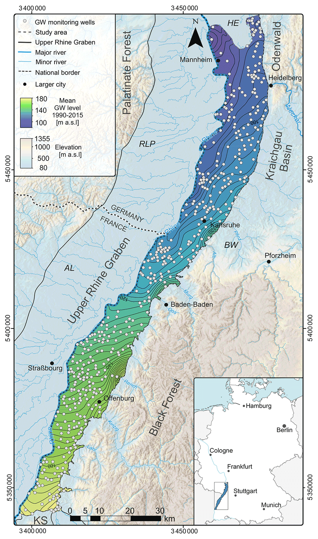
Figure 1Study area within the URG and the 480 groundwater monitoring wells used for optimization. RLP – Rhineland-Palatinate; He – Hesse; BW – Baden-Württemberg; Al – Alsace (France); KS – Kaiserstuhl volcanic complex.
2.4.2 Data and preprocessing
The data set used in this study consists of weekly GWL measurements from 480 wells in the uppermost aquifer within the Quaternary sand/gravel deposits of the URG, covering the period from 1990 to 2015 (i.e., 1304 time steps). Data values that deviate by more than ±3σ from the moving average (with a window size of 11 values) are considered outliers and were removed from further processing. Data gaps were subsequently filled based on information from highly correlated neighboring hydrographs using the clustering results of Wunsch et al. (2022). Where this did not yield plausible results or was not possible due to similarly missing data in neighboring hydrographs, an alternative PCHIP (piecewise cubic hermite interpolating polynomial) interpolation was performed. To avoid possible bias, the measurement data are globally and locally centered. The data set is split into the following two subsets: the first 80 % (January 1990–December 2009; 1043 time steps) is used to train the algorithm and the last 20 % for test/validation (January 2009–December 2014; 261 time steps). The well data are publicly available from the Baden-Württemberg State Office for Environment web service (LUBW, 2021).
2.4.3 Groundwater contour maps
We used the hydrograph data to generate 1304 weekly groundwater contour maps with a grid size of 50×50 m using ordinary kriging. In addition to finding a sparse set of monitoring wells for the optimal temporal reconstruction of other hydrographs, the objective is to identify monitoring wells that allow optimal spatiotemporal reconstruction of GWL from a subset of the wells. Moreover, the spatially continuous information of the gridded contour maps is used to suggest additional locations for an extended network. We used an isotropic Gaussian semivariogram model for interpolation, which is flexible and, therefore, a good candidate for a standard model (Krivoruchko, 2011). The associated parameters partial sill (42.7 m), range (17 853 m), lag size (1485 m), and nugget (0.05 m) were optimized using automatic cross-validation (CV) diagnostics to achieve the lowest mean square error. It should be noted that the use of a single variogram model (Gaussian) may not be the optimal way to quantify spatial correlation, especially for nonstationary data. However, this is a necessary simplification due to the automation process that still produces comparable interpolation results, while the best possible interpolation result is not the focus of this study. Just as with the hydrographs, the first 80 % (January 1990–December 2009; 1043 time steps) of the contour maps were used to train the algorithm and the last 20 % for test/validation (January 2009–December 2014; 261 time steps).
The following section is structured as follows. First, the grid search results regarding the three types of basis used, the number of basis modes, and a varying number of sensors are presented and discussed. Since we are applying the presented sensor placement approach to a groundwater monitoring well optimization, we use the term “well” as a synonym for sensors in the following. This is followed by the results of the GMN optimization based solely on the hydrograph data set. Finally, the results of the GMN optimization with the interpolated GWL as inputs are shown.

Figure 2Grid search CV results. (a) Reconstruction error (RMSE) vs. the number of monitoring wells and the number of basis modes for the three basis projections described in Sect. 2.1.3, i.e., identity (Ψr=Xtr), random projection (Ψr=GXtr), and SVD (Ψr=Utr). (b) Minimum RMSE achieved with a given number of QR-selected monitoring wells (Pareto front) and the same number of randomly selected wells (median of 100 runs; gray shading represents the total range) for comparison. (c) The corresponding number of basis modes that leads to the lowest RMSE in panel (b). Accordingly, panels (b) and (c) represent a section through panel (a) at the respective minimum on the axis of n monitoring wells.
3.1 Grid search results
Figure 2a shows the RMSE between the estimated and actual GWL for the validation set as a function of the number of wells that the network is reduced to, the type of tailored basis (identity basis, random projection, and SVD basis), and the number of basis modes used. Since the number of wells and basis modes interacts, it is necessary to determine the appropriate number of basis modes that will result in the lowest reconstruction error for a given number of wells. If the number of wells is close to the number of basis modes, the reconstruction error increases significantly for all three basis mode types used. While the number of basis modes for identity and random projection is theoretically open-ended, the dimensionality for SVD, and thus the number of basis modes, must be less than the number of wells. Although there are SVD methods (e.g., randomized SVD; Halko et al., 2011) that allow oversampling with an additional number of random vectors, our results show that the accuracy of SVD generally decreases as the number of basis modes increases, which is consistent with the findings of de Silva et al. (2021a). Therefore, we decided against an SVD method with oversampling and opted for the truncated SVD implemented in PySensors (de Silva et al., 2021a), thus using a maximum of 480 basis modes. All 1043 time steps (in the training set) were used as the maximum number of basis modes for identity and random projection. According to previous studies, the number of basis modes should be at least equal to the number of wells p+10 (de Silva et al., 2021a). Clark et al. (2019) used 2p basis modes, which in our case equals a maximum of 960 (for all 480 wells) and, thus, is covered by the maximum of 1043 basis modes in the grid search.
The results show that, with only a few basis modes, SVD has the highest accuracy (Fig. 2a). As the number of basis modes exceeds the number of remaining wells, the identity and random projection basis perform better. In general, random projection and identity basis perform similarly. With fewer than 950 basis modes, slightly better results are obtained with random projection; above 950, the identity basis performs marginally better. Figure 2b shows the lowest RMSE per number of wells achieved in the grid search, and Fig. 2c shows the corresponding number of basis modes. The gray dashed line in Fig. 2b shows the median of reconstruction errors from 100 iterations, with a random well selection as a benchmark. Except for SVD basis with fewer than 50 wells, all three basis types perform considerably better compared to reconstruction with the randomly placed wells and independently of the number of wells. Our findings are consistent with those of Manohar et al. (2018), Clark et al. (2019), and de Silva et al. (2021a), where SVD consistently underperforms compared to random projection and identity basis. However, the latter two show almost identical results with an optimized number of basis modes (Fig. 2b), with random projection performing marginally better with a small number of wells and identity basis performing slightly better with a larger number of wells. For consistency reasons, and based on the grid search results, we decided to compute the optimization steps shown in the following uniformly with identity basis and a fixed number of 1043 basis modes. This combination, on average, shows the best results for any chosen number of remaining wells (Fig. 2c).
As examples, all results of the following section are presented using five reduction stages: 10 %, 25 %, 50 %, 75 %, and 90 %. Thus, in the 25 % stage, the 25 % wells with the lowest information content are removed, and their hydrographs are predicted using the remaining optimal 75 % of the monitoring wells. The reduction stages are also shown in the grid search results (Fig. 2b and c). The color scheme of the reduction stages is kept for all remaining figures.
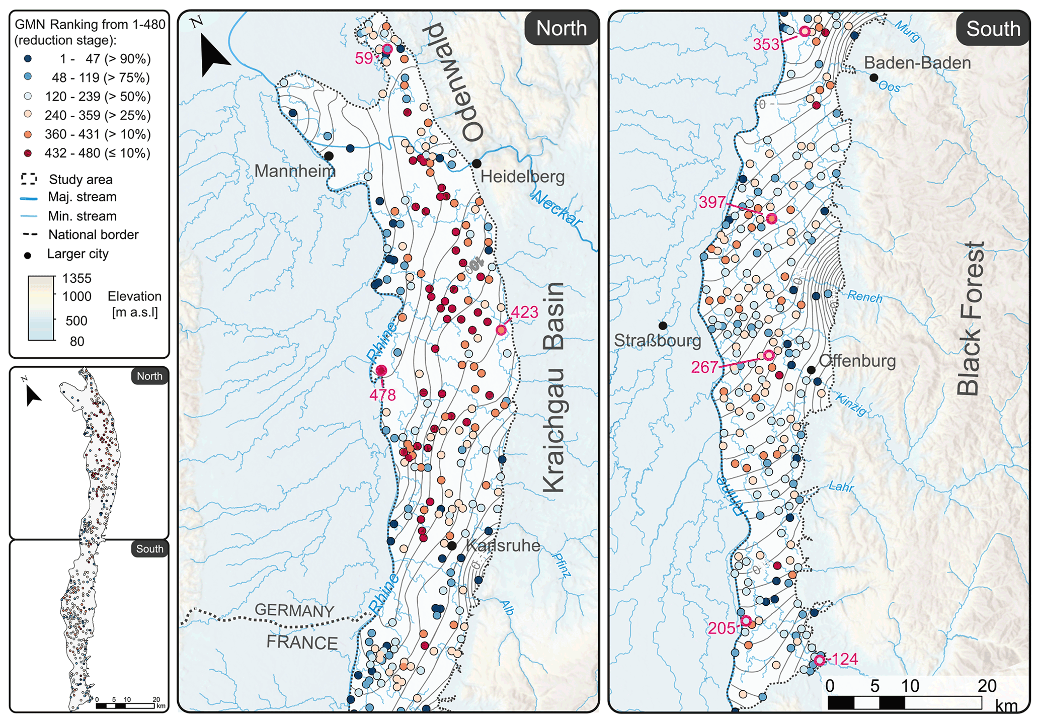
Figure 3QR-based ranking of groundwater monitoring wells based on hydrograph information content, from 1 (high information content; blue) to 480 (redundant; red). The reduction stage at which the respective wells are removed is indicated in parentheses. The hydrographs of the highlighted wells (pink) are shown in Fig. 6.
3.2 Ranking of wells and network reduction with hydrograph data
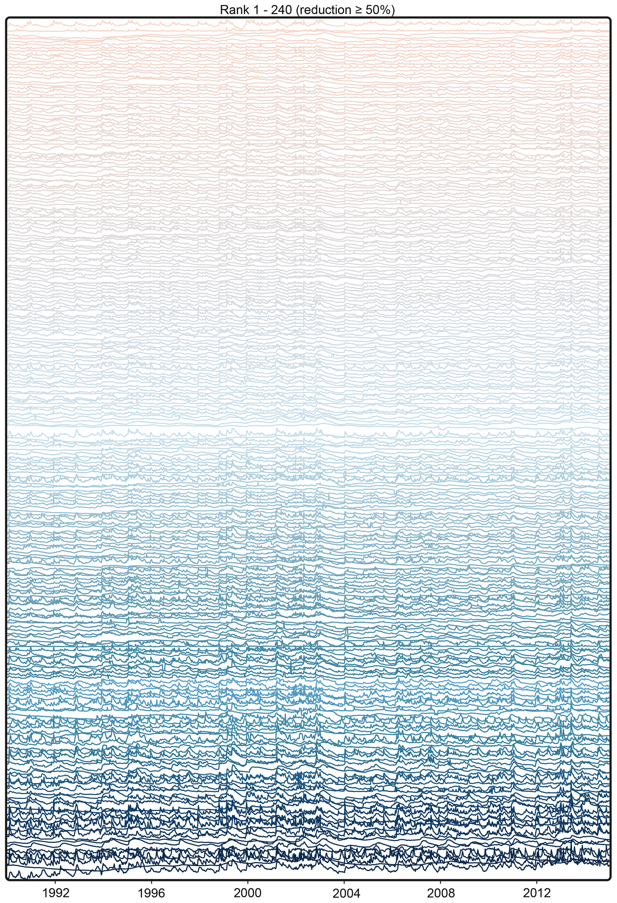
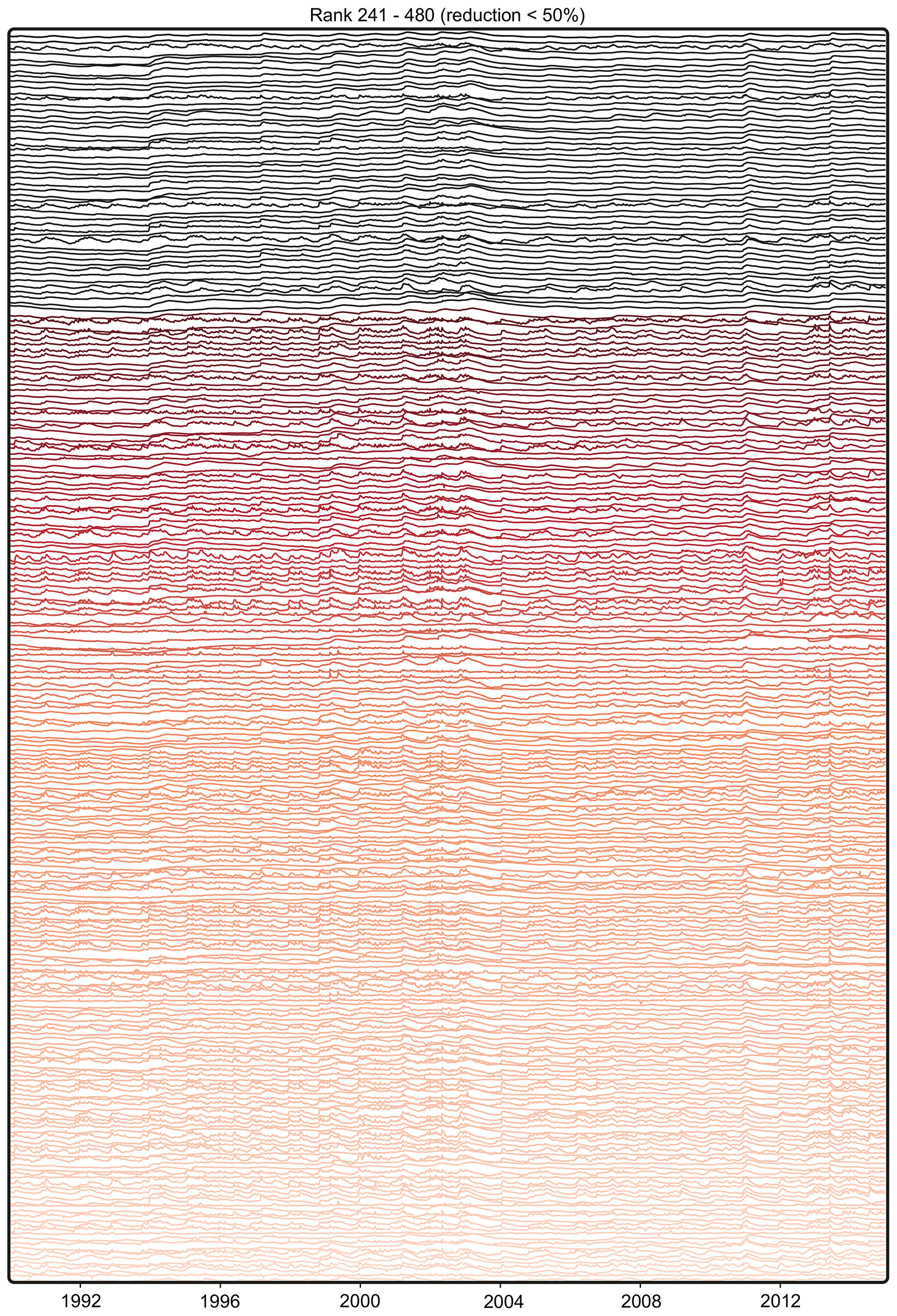
Figure 3 shows the result of the ranking of the monitoring wells computed with an identity basis and using 1043 basis modes. The ranks are assigned from 1 (essential well with high information content) to 480 (most redundant well); thus, lower numbers mean a higher ranking concerning their information content and importance to reconstructing potentially removed redundant wells. The reduction stage at which the respective wells are removed is indicated in parentheses. The color scheme ranges from dark red for redundant monitoring wells that can be eliminated with a minor loss in prediction accuracy to dark blue for important monitoring wells that contain essential information about the system and are needed for the accurate reconstruction of signals at other monitoring wells. In addition, Fig. 4 shows the centered hydrographs of the most important 10 % and the most redundant 10 % of all hydrographs. Most of the important wells (blue; removal at a reduction of >90 %) show a pronounced flashiness (i.e., high frequency and rapidity of short-term changes) and strong irregular patterns during the recording period. These dynamics indicate a strong interaction with surface waters or boundary inflows, for example, from side valleys of the rift flanks, which can also be seen in Fig. 3 from the location of the wells. Additionally, the most important wells include those with a distinct trend, which can be best seen for the two highest-ranked wells at the bottom, showing an upward trend over the considered period.
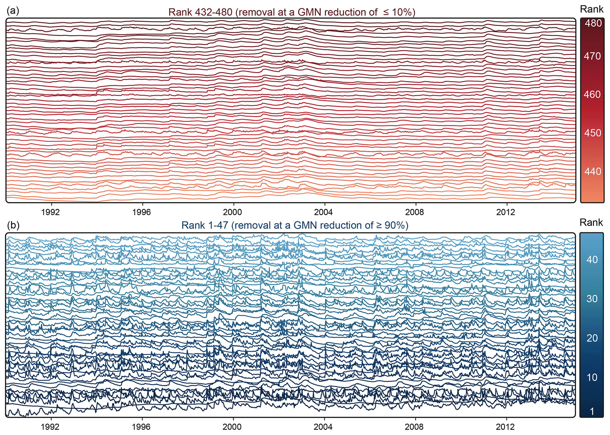
Figure 4Stacked z-transformed hydrographs of the 10 % most important monitoring wells (blue; panel b) and the 10 % most redundant monitoring wells (red; panel a). Coloring and stacked order reflect the ranking order.
In contrast, the redundant wells show low flashiness and also include wells with high seasonality, though most of the signals seem to be dominated by interannual variations. Most of these wells are located in the northern part of the study area within the URG. Since the eastern boundary in this area is the Kraichgau basin, the landscape profile is less pronounced than in the Black Forest hill range in the south and the Odenwald in the north. Therefore, less recharge occurs through stream infiltration, which is often the reason for more pronounced short-term variations or flashiness. The hydrographs of all wells can be found in the Appendix. Overall, the ranking shows that the most important wells include the ones with a noticeable unusual behavior, i.e., patterns that are not present in many of the other wells (like flashiness, trends, and jumps) and thus are hard to reconstruct. Overall, the more redundant wells either show a higher seasonality or tend to show low variability. Both patterns are common to a larger number of the wells and can be reconstructed more easily.
While the ranking itself already contains essential information and could be used, for example, to equip higher-ranked monitoring wells with higher-quality sensors or measure them with a higher time frequency, we use the ranks here to reduce the original network well by well, with most of the results shown only for the five abovementioned reduction stages, i.e., GMN reduction by 10 %, 25 %, 50 %, 75 %, and 90 %.
The upper part of Fig. 5 shows the development of the prediction accuracy of the GMN reduction for the error measures NSE, KGE, and R2 (left), as well as rBias, RMSE, and MAE (right), for the validation data set (mean and ranges of the reconstructed validation period of all predicted/removed wells). Even with only a few optimally selected wells, the predictive power is considerably higher than the mean value of the time series (NSE = 0). An average performance for the validation period of all predicted removed wells rated as satisfactory (NSE > 0.5) is already achieved with only nine remaining wells (corresponds to a reduction of 98.1 %), those rated as good (NSE > 0.65) with 21 remaining wells (95.6 %), and those rated as very good (NSE > 0.75) with 54 remaining wells (88.7 %). With more than 191 wells (60.2 %), the NSE rises above 0.9. KGE and R2 behave in much the same way as NSE. A KGE of 0.75 is achieved with nine wells (98.1 %) and 0.9 with 144 wells (70.0 %). R2 of 0.75 is achieved with 22 wells (95.4 %) and of 0.9 with 155 wells (67.7 %), respectively. A MAE of 0.1 m is achieved with 31 monitoring wells (93.5 %) remaining, 0.05 m with 147 wells (69.4 %), and 0.01 m with 394 wells (17.9 %). From a reduction of more than about 75 %, the removal of each subsequent well leads to a disproportionate decrease in accuracy, with a very steep drop from about 95 % on. When the reduction is less than 75 %, the gradient shows a nearly linear course, meaning a linear (but small) performance increase with more monitoring wells. The rBias also approaches zero at a reduction below 75 %. Thus, we conclude that about 25 % of the wells could be seen as a kind of absolute minimum that is required to adequately describe the system dynamics in the considered study area, despite the average NSE of the reconstruction still being rated as good for only the optimally selected 10 % of the wells.

Figure 5(a) Reconstruction error metrics (KGE, R2, NSE, MAE, RMSE, and rBias) as a function of the number of QR-ranked remaining monitoring wells for the identity basis and 1043 basis modes (lines are mean values, and shading represents the total range of reconstruction errors over all removed wells). (b) Same reconstruction error metrics with a GMN reduction of 10 %, 25 %, 50 %, 75 %, and 90 %, as boxplots, compared to the same number of randomly removed wells (gray).
The lower part of Fig. 5 displays the performance of the QR-optimized wells compared to an equal number of randomly selected remaining wells for a reduction by 10 % (48 wells) to 90% (432 wells) of the GMN. Removing wells based on the ranking results leads to a lower prediction loss. Only at a reduction of more than 90 % are the errors in the same range as for the randomly removed wells. Therefore, the information content of these 10 % remaining wells is probably not sufficient to reflect the overall dynamics. Again, from about 75 % downwards, the performance differences become more pronounced, with a considerably higher average, 25 % quantile, and minimum NSE, KGE, and R2 values (lower MAE and RMSE, respectively). Below a reduction of 25 %, the 75 % quantile and minimum NSE, KGE, and R2 values are also clearly higher (lower for MAE and RMSE, respectively). This clearly shows that the advantages of the data-driven optimization method come into play, especially for moderate to smaller reductions of a GMN.
Figure 6 shows the temporal reconstruction accuracy at the considered reduction stages from 10 % to 90 % for eight selected wells (see also Fig. 3). These wells were chosen to reflect the dynamics spectrum and represent the full ranking range. The reconstruction is always based on the higher-ranked remaining wells (but keeping the chosen reduction stages). Consequently, well 154-304-1, the highest-ranked well shown with rank 59 (bottom), which could theoretically be reconstructed with a maximum of 58 remaining wells, is reconstructed with 10 % of the wells (48). Similarly, well 132-257-4, the lowest-ranked well with rank 478 (top), which could theoretically be reconstructed with a maximum of 477 wells, is reconstructed with 90 %, 75 %, 50 %, 25 %, and 10 % remaining wells (432, 360, 240, 120, and 48, respectively) for a comparison.
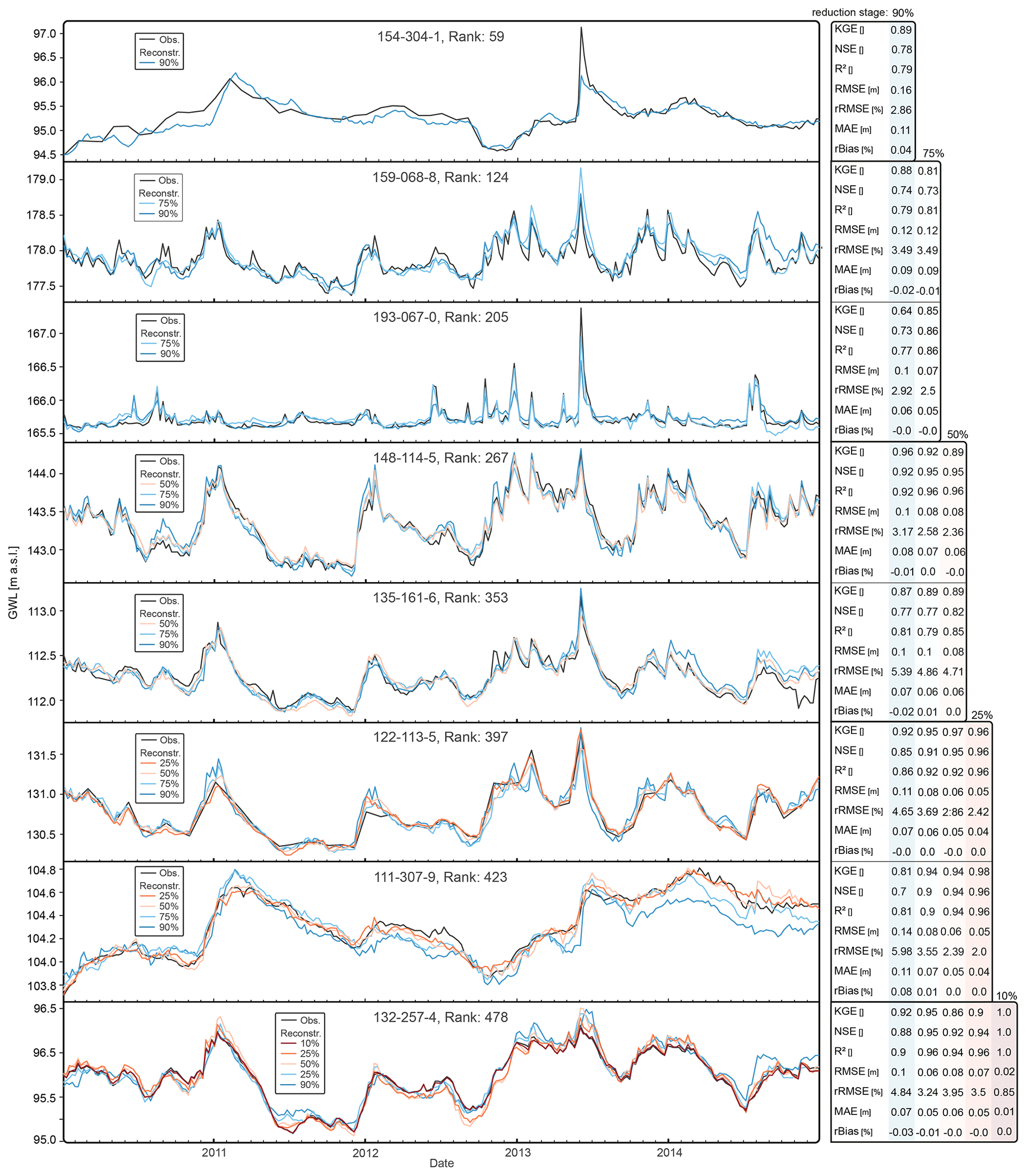
Figure 6Hydrograph reconstruction at the five reduction stages 10 %–90 % shown for eight monitoring wells, along with the respective error measures.
The results show that the individual dynamics of the hydrographs can already be adequately reconstructed with a 10 % subset of the monitoring network. As expected, as the number of wells increases, the accuracy improves on average, hydrographs are reproduced more consistently, and short-term peaks are reproduced more accurately. Though these seem to be only, comparatively, slight improvements, considering the overall dynamics for some wells and time steps, the absolute errors can be up to several tens of centimeters, albeit achieved by many additional wells. Whether this justifies the increased operating costs of the monitoring network depends on the task at hand. The reconstruction results for the other wells can be found in the Appendix.
3.3 Network reduction and extension based on gridded GWL contour maps
This application case is based on spatially continuous gridded weekly GWL contour maps from 1990 to 2015. Analogous to the hydrograph data set, the first 80 % of this period was used for model training and the last 20 % for evaluation. According to the ranking, we investigate how well the GWL can be reconstructed with two reduction stages in which 10 % and 20 % of the GMN are removed. We have selected these reduction stages since, in the analysis of the reduction stages with hydrographs, the advantages of the data-driven optimization method were more pronounced for moderate to smaller reductions of a GMN. Moreover, reducing an existing network by more than 20 % seems unrealistic in practice. Furthermore, we extend the existing network by 10 % and 20 % wells and analyze where new wells are placed to supposedly improve the GMN. To account for more or less suitable locations (e.g., with regard to infrastructure), we apply costs with a non-uniform spatial step function on a 50×50 grid (corresponding to the used GWL grid) into the QR factorization. The cost function grid is assigned zero (no additional costs) at existing monitoring well locations to ensure that existing wells remain since, technically, the extension (by e.g., 10 %) is realized such that 110 % of new wells are placed on the gridded GWL maps. At potentially well-suited additional sites, which are defined within 50 m of roads and paths, outside surface waters, and where the slope is less than 20 %, we assigned a cost value of 21. For all other areas that are considered as not suitable, the cost weighting is set to 22. Alternatively, a gradual cost function can be used, where the weighting increases with distance to the infrastructure or similar. It should be noted that the weighting depends on the system, basis, and cost function and must be adjusted for the particular case (Clark et al., 2019). We assigned the mentioned weighting factors iteratively until it resulted in the desired behavior. With the weightings chosen in this way, it was possible to achieve a result such that the first 480 wells are placed at existing monitoring wells, and all subsequent wells are placed at suitable locations, while the algorithm avoids the other locations. Finally, we combine a reduction/extension scenario, where the original number of wells is kept, but the 10 % and 20 % most redundant wells are removed and replaced afterward. Technically, this is done in a two-step procedure, consisting of the reduction step followed by the above-described extension, where the cost function is adapted for the existing wells.
The maps on the left side of Fig. 7a show the spatial distribution of the monitoring wells as a result of a 10 % (yellow dots) and 20 % (red dots) reduction (1), and a 10 % (light blue dots) and 20 % (dark blue dots) extension (2) of the GMN, as well as a combined reduction/extension of the GMN (3). For the latter, redundant 10 % and 20 % monitoring wells were eliminated and replaced with wells at optimal locations. We should note that the ranking based on the spatially interpolated data is different from the ranking based on the hydrographs alone (see Appendix A).
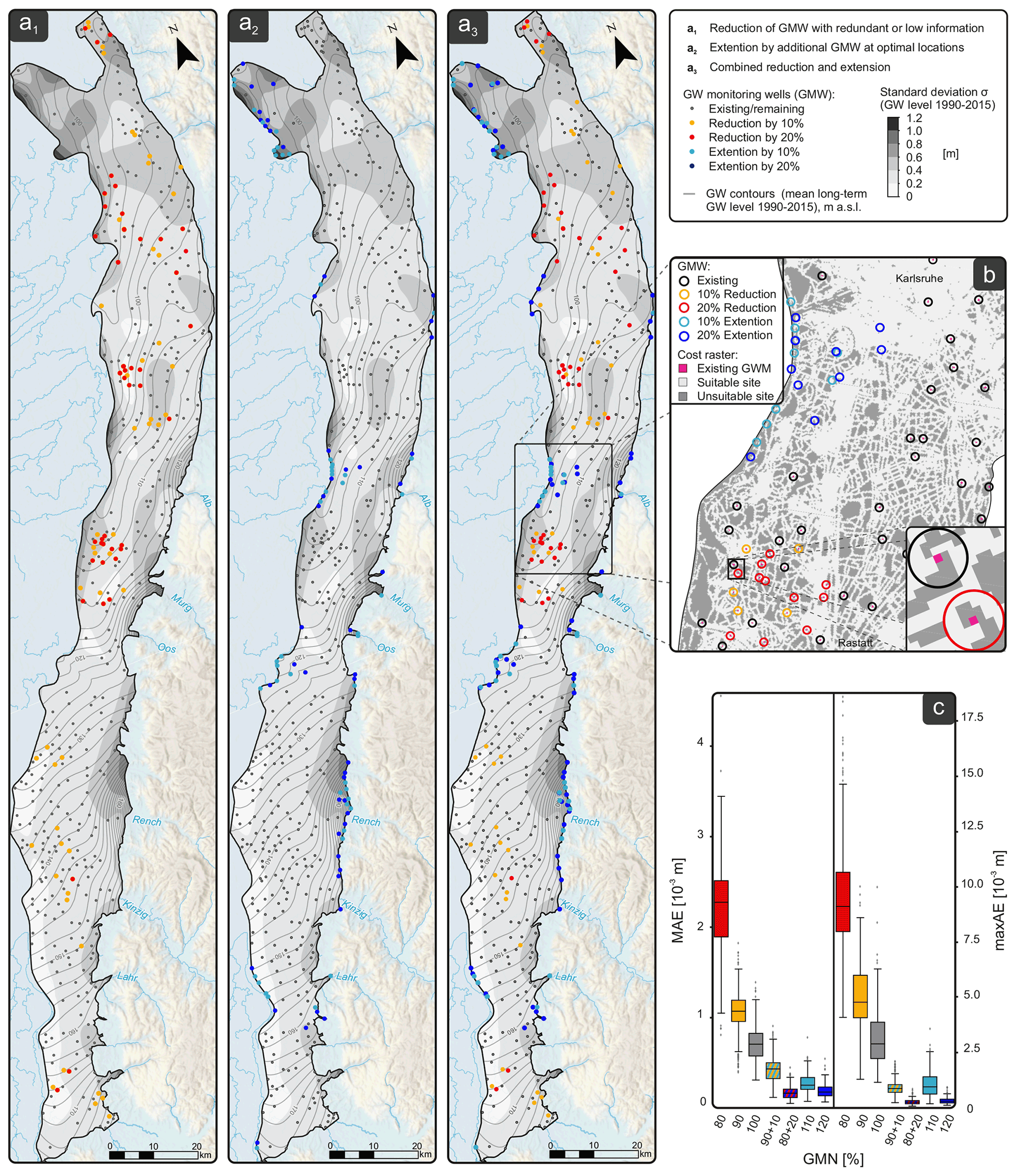
Figure 7(a) Location of removed groundwater monitoring wells (GMWs) in a 10 % (yellow) and 20 % (red) QR-based monitoring well reduction (left map; panel a1), in a 10 % (light blue) and 20 % extension (center map, a2), and in a combined reduction/extension in which 10 % and 20 %, respectively, of the monitoring wells were removed and replaced with wells at optimal locations (right map; panel a3). (b) Cost function grid used for the GMN extension. (c) Box plots show the mean and maximum absolute error of the reconstruction of the 216 GWL contour maps of the test set obtained with the mentioned GMN reduction/extension.
This variation can be explained by the ranking reflecting the information content regarding the reconstruction with the lowest possible error. While, in the case of hydrographs, the goal is to reconstruct the hydrographs of the removed wells, here the goal is to reconstruct the interpolated surface (which constitutes a best guess of spatially continuous GWL based on the available data).
While the first 10 % of reduced wells are evenly distributed across the study area, the subsequent removal step (i.e., additional 10 %; thus, 20 % removed wells in total) eliminates well clusters in the central and northern regions. This seems conclusive because clusters of nearby wells tend to show similar dynamics and thus do not add much information to an interpolation, according to Tobler's law. Optimal locations for additional wells are identified primarily along the western and eastern margins, i.e., along the Rhine and downstream of the alluvial valley aquifers of the adjacent Black Forest. These are areas with expected higher groundwater dynamics (e.g., high seasonal magnitudes and high flashiness) and, on the other hand, due to the elongated geometry of the URG, areas with increased interpolation uncertainty (transition from interpolation to extrapolation). Optimal well locations are primarily, but not exclusively, located in areas of increased variability (standard deviation of the interpolated GWL; see Fig. 7a2 and a3).
The box plots in Fig. 7c show the mean (left) and maximum (right) absolute error of the reconstructed 261 GWL contour maps of the evaluation set for all abovementioned scenarios. It has to be noted that the MAE is now taken as the mean over the spatial axis, i.e., for each of the reconstructed 261 GWL contour maps separately (whereas, with the hydrographs, the MAE was taken as the mean over the time axis for each reconstructed well). This was done because, in the application case, the focus is on the error of a spatial reconstruction of GWL contours and not explicitly on time series. Correspondingly, the maximum absolute error (maxAE) is the maximum over the spatial axis for each of the reconstructed 261 GWL contour maps. We therefore also refer to them as mean and maximum spatial reconstruction errors. Thus, the boxes in Fig. 7c show the variability in the mean absolute error and maximum absolute error over the 261 time steps.
On average, the model can reconstruct the GWL contour maps with very high accuracy, with mean absolute errors far below 1 cm. This seems very low compared to the reconstruction of the hydrographs. However, this is due to the fact that the reconstruction of a large number of many similar values (i.e. raster pixels) is much easier for the model, for the following two reasons: (i) there are many more training patterns for each type of dynamics than with the hydrographs alone, and (ii) the overall dynamics are reduced by the interpolation itself, which smooths the data spatially and temporally. Taking these limitations due to spatially interpolated data into account, it seems more reasonable to focus on the maximum absolute error, which allows the identification of areas with higher errors, where the model (with the existing data) cannot produce reliable reconstructions and additional wells would bring the most information.
When comparing the maxAE (Fig. 7c; right) for all scenarios, we see that a reduction in the network increases the spatial reconstruction error by a factor of about 2 for 10 % reduction and about 3 to 4 for 20 %. For comparison, the gray box (100 %) shows the reconstruction errors with an unchanged GMN (this error results from the fact that the model is trained with the first 80 % of all time steps, but the reconstruction is performed for the unknown 20 % of the evaluation data set). An extension of the network by 10 % can considerably reduce the spatial reconstruction error to about less than two-thirds, while an extension by 20 % reduces it further to 1/10 of the initial value. Most interestingly, the reconstruction errors for the combined reduction/extension scenarios with 90 %/10 % and 80 %/20 %, respectively (thus an unchanged number of 480 wells in total), are slightly below the straightforward GMN extension with 110 % (528 wells) and 120 % (576 wells). To a lesser degree, this also applies to the mean absolute errors, at least for the 80 %/20 % scenario, which performs slightly better than an extension by 20 %, and considerably better than a 10 % extension. In practice, that means that, with a combined reduction/extension, for example, sensors/data loggers that become available can be used elsewhere at better locations. This reduces the installation costs of the additional wells and the operating costs of the GMN and, moreover, performs about the same as or even better than a pure extension.
This study investigated data-driven sparse sensing approaches based on the work of de Silva et al. (2021a), Clark et al. (2019), and Manohar et al. (2018) and adapted them to optimize an existing GLMN. The algorithm fits a tailored basis to the training data, subsequently used in a QR decomposition to rank the monitoring wells by importance based on reconstruction performance. This approach allows us to remove groundwater monitoring wells with low information content if needed, equip monitoring wells with higher rank with higher quality sensors, or measure with a higher time frequency. When using spatially continuous input data (by interpolation or numerical simulation), the ranking is performed according to the same scheme for all locations. This rank can be used as a decision-making aid to search for locations for additional monitoring wells. We incorporated a cost function to eliminate inaccessible locations from the site selection process. Adjusting the cost constraint allows a specific adaptation to the individual problem definition.
Our results show that identifying redundant, low-ranking monitoring sites would allow a drastic reduction of the monitoring network, with a minor loss of information, compared to a random reduction (which corresponds to a reduction based on other criteria, as is often the case in practice). In the case of a desired network extension, the reconstruction quality can benefit from the additional removal of unsuitable wells.
As in related previous studies (Clark et al., 2019; Manohar et al., 2018), using the identity data basis (raw data without dimensionality reduction) and the total number of available base modes yielded a lower reconstruction error for a given number of wells compared to other basis mode types and numbers. This is because no information is lost when constructing a low-ranking approximation to the data. However, for larger data sets than the one used in this study, an optimization without previous dimensionality reduction can lead to impractically long computation times. Just as in the work of Clark et al. (2019) and Manohar et al. (2018), a randomized projection of the data in our study performed, on average, only slightly worse than the raw data and may be worthwhile for large data sets or multiple computational runs due to lower computational costs. Even though the widely used SVD basis gave the worst results for our data set, the reconstruction errors are still lower than for a random network optimization.
In addition to GLMN, this approach can also optimize groundwater quality or multivariate monitoring networks. As with all data-driven methods, the quality of the results depends strongly on the availability of the input data (spatial and primarily temporal). Since this approach relies on detecting patterns in data and placing monitoring locations based on those patterns, it benefits from large data sets. Therefore, we see the main application of this technique in optimizing monitoring networks of regional-scale groundwater systems, where a comprehensive overview of the variability and quantity of groundwater bodies and the assessment of long-term changes in natural conditions is the monitoring objective.
Overall, we could demonstrate that modern data-driven methods of sparse sensing are well suited for the application to groundwater monitoring networks, as long as there is a good historic data basis. The applied method can be used for an optimization regarding the number of wells and their location, for a network reduction and extension, or for both combined. Using hydrographs (1D) as input data, the applied approach allows an information-based assessment of an operated monitoring network. The outcomes can be used to identify representative key wells for selecting expressive subnetworks, equip the critical wells with improved data loggers, or release installed sensors/loggers at redundant wells for more suitable locations. The spatial dependency structures and the sphere of influence of wells can be considered in optimizing with two-dimensional input data, both for reduction and for an extension of monitoring networks tailored to the dynamics of the aquifer. Although optimized reduction can generally lead to greater cost efficiency, it should always be done judiciously and in combination with expert knowledge of the system.
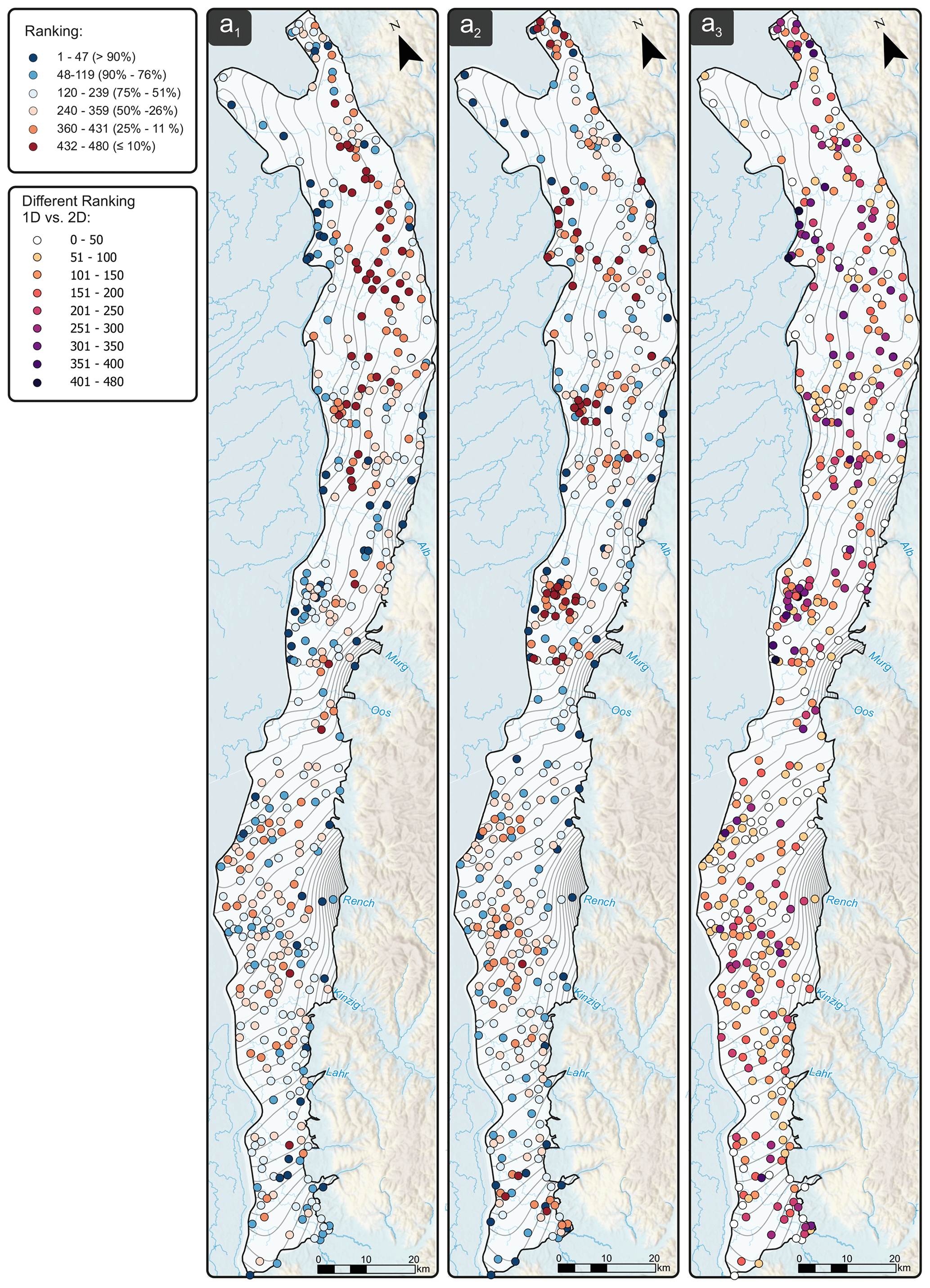
Figure A1Comparison of QR-based ranking with 1D hydrograph data (left; panel a1), with 2D interpolated GWL contour maps (middle; panel a2) and differences of rankings between 1D and 2D (right; panel a3).
| Abbreviations | |
| CV | Cross validation |
| GA | Genetic algorithm |
| GLMN | Groundwater level monitoring network |
| GMN | Groundwater monitoring network |
| GQMN | Groundwater quality monitoring network |
| GWL | Groundwater level |
| GMW | Groundwater monitoring well |
| KGE | Kling–Gupta efficiency |
| MAE | Mean absolute error |
| maxAE | Maximum absolute error |
| NSE | Nash–Sutcliffe efficiency |
| R2 | Coefficient of determination here: squared |
| Pearson r | |
| PCA | Principal component analysis |
| POD | Proper orthogonal decomposition |
| rBias | Relative bias |
| rRMSE | Relative root mean square error |
| RMSE | Root mean square error |
| SVD | Singular value decomposition |
| URG | Upper Rhine Graben |
| WFD | Water Framework Directive |
| ND | Nitrates Directive |
The work is based on the methodology developed by de Silva et al. (2021a), Manohar et al. (2018), and Clark et al. (2019), for optimized sensor placement implemented in PySensors and is available at https://doi.org/10.5281/zenodo.4542530 (de Silva et al., 2021b). The well data are publicly available from the web service of the Baden-Württemberg State Office for Environment (LUBW, 2021). Our customized code files for the optimization of groundwater monitoring networks are available in Ohmer (2022).
MO was responsible for the conceptualization, methodology, software, formal analysis, validation, investigation, visualization, and preparing the original draft. TL was responsible for the conceptualization, methodology, and review and editing of the paper and also supervised. AW preprocessed and curated the data and assisted with the review and editing of the paper.
The contact author has declared that none of the authors has any competing interests.
Publisher's note: Copernicus Publications remains neutral with regard to jurisdictional claims in published maps and institutional affiliations.
This study is a contribution to the project “Nitrate Monitoring 4.0 – Intelligent Systems for Sustainable Reduction of Nitrate in Groundwater (NiMo 4.0)”, funded by the German Federal Ministry for the Environment, Nature Conservation, and Nuclear Safety (BMU) on the basis of a resolution of the German Federal Parliament. We thank all colleagues in the project, for valuable discussions.
The article processing charges for this open-access publication were covered by the Karlsruhe Institute of Technology (KIT).
This paper was edited by Mauro Giudici and reviewed by Alper Elci and Hugo Loaiciga.
Alizadeh, Z. and Mahjouri, N.: A spatiotemporal Bayesian maximum entropy-based methodology for dealing with sparse data in revising groundwater quality monitoring networks: the Tehran region experience, Environ. Earth Sci., 76, 436, https://doi.org/10.1007/s12665-017-6767-6, 2017. a
Alizadeh, Z., Yazdi, J., and Moridi, A.: Development of an Entropy Method for Groundwater Quality Monitoring Network Design, Environ. Process., 5, 769–788, https://doi.org/10.1007/s40710-018-0335-2, 2018. a
Ammar, K., Khalil, A., McKee, M., and Kaluarachchi, J.: Bayesian deduction for redundancy detection in groundwater quality monitoring networks, Water Resour. Res., 44, W08412, https://doi.org/10.1029/2006WR005616, 2008. a
Annoni, J., Taylor, T., Bay, C., Johnson, K., Pao, L., Fleming, P., and Dykes, K.: Sparse-Sensor Placement for Wind Farm Control, J. Phys.: Conf. Ser., 1037, W08412, https://doi.org/10.1088/1742-6596/1037/3/032019, 2018. a, b
Asefa, T., Kemblowski, M. W., Urroz, G., McKee, M., and Khalil, A.: Support vectors-based groundwater head observation networks design, Water Resour. Res., 40, W11509, https://doi.org/10.1029/2004WR003304, 2004. a
Ayvaz, M. T. and Elçi, A.: Identification of the optimum groundwater quality monitoring network using a genetic algorithm based optimization approach, J. Hydrol., 563, 1078–1091, https://doi.org/10.1016/j.jhydrol.2018.06.006, 2018. a
Baraniuk, R.: A Lecture on Compressive Sensing v, IEEE signal processing magazine, 24.4, 118–121, 2007. a, b
Bashi-Azghadi, S. N. and Kerachian, R.: Locating monitoring wells in groundwater systems using embedded optimization and simulation models, Sci. Total Environ., 408, 2189–2198, https://doi.org/10.1016/j.scitotenv.2010.02.004, 2010. a
Bhat, S., Motz, L. H., Pathak, C., and Kuebler, L.: Geostatistics-based groundwater-level monitoring network design and its application to the Upper Floridan aquifer, USA, Environ. Monit. Assess., 187, 4183, https://doi.org/10.1007/s10661-014-4183-x, 2015. a
Brunton, B. W., Brunton, S. L., Proctor, J. L., and Kutz, J. N.: Sparse Sensor Placement Optimization for Classification, SIAM J. Appl. Math., 76, 2099–2122, https://doi.org/10.1137/15M1036713, 2016. a, b
Brunton, S. L. and Kutz, J. N.: Data-driven Science and Engineering: Machine Learning, Dynamical Systems, and Control, Cambridge University Press, https://doi.org/10.1017/9781108380690, 2017. a, b, c
Candes, E. and Wakin, M.: An Introduction To Compressive Sampling, IEEE Signal Process. Mag., 25, 21–30, https://doi.org/10.1109/MSP.2007.914731, 2008. a, b
Candes, E., Romberg, J., and Tao, T.: Stable Signal Recovery from Incomplete and Inaccurate Measurements, arXiv:math/0503066, p. 15castillo, https://doi.org/10.48550/arXiv.math/0503066, 2005. a, b
Castillo, A. and Messina, A. R.: Data‐driven sensor placement for state reconstruction via POD analysis, IET Generat. Transmiss. Distribut., 14, 656–664, https://doi.org/10.1049/iet-gtd.2019.0199, 2020. a
Clark, E., Askham, T., Brunton, S. L., and Nathan Kutz, J.: Greedy Sensor Placement With Cost Constraints, IEEE Sensors J., 19, 2642–2656, https://doi.org/10.1109/JSEN.2018.2887044, 2019. a, b, c, d, e, f, g, h, i, j, k
Dasgupta, S.: Experiments with Random Projection, in: Proceedings of the Sixteenth Conference on Uncertainty in Artificial Intelligence, 30 June–3 July 2000, Stanford, 143–151, 2000. a
De Jesus, K. L. M., Senoro, D. B., Dela Cruz, J. C., and Chan, E. B.: A Hybrid Neural Network-Particle Swarm Optimization Informed Spatial Interpolation Technique for Groundwater Quality Mapping in a Small Island Province of the Philippines, Toxics, 9, 273, https://doi.org/10.3390/toxics9110273, 2021. a
Derer, C. E.: Tectono-sedimentary evolution of the northern Upper Rhine Graben (Germany), with special regard to the early syn-rift stage, PhD thesis, Rheinischen Friedrich-Wilhelms-Universität Bonn, Bonn, https://nbn-resolving.org/urn:nbn:de:hbz:5n-02633 (last access: 3 August 2022), 2003. a
de Silva, B. M., Manohar, K., Clark, E., Brunton, B. W., Brunton, S. L., and Kutz, J. N.: PySensors: A Python Package for Sparse Sensor Placement, J. of Open Source Softw., 6, 2828, https://doi.org/10.21105/joss.02828, 2021a. a, b, c, d, e, f, g, h
de Silva, B. M., Manohar, K., Clark, E., Brunton, B. W., Kutz, J. N., and Brunton, S. L.: PySensors: A Python Package for Sparse Sensor Placement (v0.3.3), Zenodo [code], https://doi.org/10.5281/zenodo.4542530, 2021b. a
Dhar, A. and Patil, R. S.: Multiobjective Design of Groundwater Monitoring Network Under Epistemic Uncertainty, Water Resour. Manage., 26, 1809–1825, https://doi.org/10.1007/s11269-012-9988-1, 2012. a
Donoho, D.: Compressed sensing, IEEE T. Inform. Theory, 52, 1289–1306, https://doi.org/10.1109/TIT.2006.871582, 2006. a
EC: Council Directive 91/676/EC of 12 December 1991 concerning the protection of waters against pollution caused by nitrates from agricultural sources, Official Journal of the European Communities, L375, Vol. 34, ISSN 0378-6978, 1991. a
EC: Directive 2000/60/EC of the European Parliament and of the Council of 23 October 2000 establishing a framework for Community action in the field of water policy, Official Journal of the European Communities, L 327, Vol. 43, ISSN 0378-6978, 2000. a
Emmert, M., Zigelli, N., Haakh, F., Bode, F., and Nowak, W.: Risikiobasiertes Grundwassermonitoring für Wasserschutzgebiete, energie/wasser-praxis, 68–73, https://www.dvgw.de/medien/dvgw/sicherheit/wasser/ewp-risikomanagement-wasserschutzgebiete (last access: 3 August 2022), 2016. a
Gaur, S., Ch, S., Graillot, D., Chahar, B. R., and Kumar, D. N.: Application of Artificial Neural Networks and Particle Swarm Optimization for the Management of Groundwater Resources, Water Resour. Manage., 27, 927–941, https://doi.org/10.1007/s11269-012-0226-7, 2013. a
Golub, G. and Kahan, W.: Calculating the Singular Value and Pseudo-Inverse of a Matrix, J. SIAM Numer. Anal. Ser. B, 2, 205–224, 1965. a
Guneshwor, L., Eldho, T. I., and Vinod Kumar, A.: Identification of Groundwater Contamination Sources Using Meshfree RPCM Simulation and Particle Swarm Optimization, Water Resour. Manage., 32, 1517–1538, https://doi.org/10.1007/s11269-017-1885-1, 2018. a
Gupta, H. V., Sorooshian, S., and Yapo, P. O.: Status of Automatic Calibration for Hydrologic Models: Comparison with Multilevel Expert Calibration, J. Hydrol. Eng., 4, 135–143, https://doi.org/10.1061/(ASCE)1084-0699(1999)4:2(135), 1999. a
Gupta, H. V., Kling, H., Yilmaz, K. K., and Martinez, G. F.: Decomposition of the mean squared error and NSE performance criteria: Implications for improving hydrological modelling, J. Hydrol., 377, 80–91, https://doi.org/10.1016/j.jhydrol.2009.08.003, 2009. a
Halko, N., Martinsson, P.-G., and Tropp, J. A.: Finding structure with randomness: Probabilistic algorithms for constructing approximate matrix decompositions, SIAM Rev., Survey and Review section, 53, 217–288, https://doi.org/10.48550/arXiv.0909.4061, 2011. a, b, c
Hosseini, M. and Kerachian, R.: A Bayesian maximum entropy-based methodology for optimal spatiotemporal design of groundwater monitoring networks, Environ. Monit. Assess., 189, 433, https://doi.org/10.1007/s10661-017-6129-6, 2017. a
Hussain, Z. and Muhammad, A.: Sample size reduction in groundwater surveys via sparse data assimilation, in: 2013 IEEE 10th International Conference on Networking, Sensing and Control (ICNSC 2013), 10–12 April 2013, Evry, France, 176–182, https://doi.org/10.1109/ICNSC.2013.6548732, 2013. a
Júnez-Ferreira, H. E., Herrera, G. S., González-Hita, L., Cardona, A., and Mora-Rodríguez, J.: Optimal design of monitoring networks for multiple groundwater quality parameters using a Kalman filter: application to the Irapuato-Valle aquifer, Environ. Monit. Assess., 188, 39, https://doi.org/10.1007/s10661-015-5036-y, 2016. a
Keum, J., Kornelsen, K., Leach, J., and Coulibaly, P.: Entropy Applications to Water Monitoring Network Design: A Review, Entropy, 19, 613, https://doi.org/10.3390/e19110613, 2017. a
Khader, A. I. and McKee, M.: Use of a relevance vector machine for groundwater quality monitoring network design under uncertainty, Environ. Model. Softw., 57, 115–126, https://doi.org/10.1016/j.envsoft.2014.02.015, 2014. a
Khalil, A., Almasri, M. N., McKee, M., and Kaluarachchi, J. J.: Applicability of statistical learning algorithms in groundwater quality modeling, Water Resour. Res., 41, W05010, https://doi.org/10.1029/2004WR003608, 2005. a
Kim, K.-H. and Lee, K.-K.: Optimization of groundwater-monitoring networks for identification of the distribution of a contaminant plume, Stoch. Environ. Res. Risk A., 21, 785–794, https://doi.org/10.1007/s00477-006-0094-x, 2007. a
Knoben, W. J. M., Freer, J. E., and Woods, R. A.: Technical note: Inherent benchmark or not? Comparing Nash–Sutcliffe and Kling–Gupta efficiency scores, Hydrol. Earth Syst. Sci., 23, 4323–4331, https://doi.org/10.5194/hess-23-4323-2019, 2019. a, b
Kollat, J., Reed, P., and Maxwell, R.: Many-objective groundwater monitoring network design using bias-aware ensemble Kalman filtering, evolutionary optimization, and visual analytics, Water Resour. Res., 47, W02529, https://doi.org/10.1029/2010WR009194, 2011. a
Komasi, M. and Goudarzi, H.: Multi-objective optimization of groundwater monitoring network using a probability Pareto genetic algorithm and entropy method (case study: Silakhor plain), J. Hydroinform., 23, 136–150, https://doi.org/10.2166/hydro.2020.061, 2021. a
Krivoruchko, K.: Spatial Statistical Data Analysis for GIS Users, Esri Press, Redlands, California, https://downloads.esri.com/esripress/pdfs/spatial-statistical-data-analysis-for-gis-users.pdf (last access: 3 August 2022), 2011. a
Lee, T.-W., Lee, J. Y., Park, J. E., Bellerova, H., and Raudensky, M.: Reconstructive Mapping from Sparsely-Sampled Groundwater Data Using Compressive Sensing, J. Geogr. Inform. Syst., 13, 287–301, https://doi.org/10.4236/jgis.2021.133016, 2021. a
Li, J., Bárdossy, A., Guenni, L., and Liu, M.: A Copula based observation network design approach, Environ. Model. Softw., 26, 1349–1357, https://doi.org/10.1016/j.envsoft.2011.05.001, 2011. a
Li, P., Hastie, T. J., and Church, K. W.: Very sparse random projections, in: Proceedings of the 12th ACM SIGKDD international conference on Knowledge discovery and data mining – KDD'06, ACM Press, Philadelphia, PA, USA, p. 287, https://doi.org/10.1145/1150402.1150436, 2006. a
Loaiciga, H. A., Charbeneau, R. J., Everett, L. G., Fogg, G. E., Hobbs, B. F., and Rouhani, S.: Review of Ground-Water Quality Monitoring Network Design, J. Hydraul. Eng., 118, 11–37, https://doi.org/10.1061/(ASCE)0733-9429(1992)118:1(11), 1992. a
LUBW: Hydrogeologischer Bau und hydraulische Eigenschaften – INTERREG III A-Projekt MoNit “Modellierung der Grundwasserbelastung durch Nitrat im Oberrheingraben”, https://pudi.lubw.de/detailseite/-/publication/92102-INTERREG_III_A-Projekt_MoNit__Modellierung_der_Grundwasserbelastung_durch_Nitrat_im_Oberrheingraben_.pdf (last access: 3 August 2022), 2006. a
LUBW: Umwelt-Daten und -Karten Online (UDO), https://udo.lubw.baden-wuerttemberg.de/public/ (last access: 3 August 2022), 2021. a, b
Manohar, K., Brunton, B., Kutz, K., and Brunton, S.: Data-Driven Sparse Sensor Placement for Reconstruction: Demonstrating the Benefits of Exploiting Known Patterns, IEEE Control Syst., 38, 63–86, https://doi.org/10.1109/MCS.2018.2810460, 2018. a, b, c, d, e, f, g, h
Moore, G. E.: Cramming more components onto integrated circuits, Proc. IEEE, 86, 82–85, 1998. a
Moriasi, D., Arnold, J. G., Liew, M. W. V., Bingner, R. L., Harmel, R. D., and Veith, T. L.: Model Evaluation Guidelines for Systematic Quantification of Accuracy in Watershed Simulations, T. ASABE, 50, 885–900, https://doi.org/10.13031/2013.23153, 2007. a
Nash, J. and Sutcliffe, J.: River flow forecasting through conceptual models part I – A discussion of principles, J. Hydrol., 10, 282–290, https://doi.org/10.1016/0022-1694(70)90255-6, 1970. a
Nunes, L. M., Cunha, M. C., and Ribeiro, L.: Groundwater Monitoring Network Optimization with Redundancy Reduction, J. Water Resour. Pl. Manage., 130, 33–43, https://doi.org/10.1061/(ASCE)0733-9496(2004)130:1(33), 2004. a
Ohmer, M.: marcohmer/GMNO: Initial Release, Zenodo [code], https://doi.org/10.5281/zenodo.6075863, 2022. a
Ohmer, M., Liesch, T., and Goldscheider, N.: On the Optimal Spatial Design for Groundwater Level Monitoring Networks, Water Resour. Res., 55, 9454–9473, https://doi.org/10.1029/2019WR025728, 2019. a
Pollard, A., Castillo, L., Danaila, L., and Glauser, M. (Eds.): Whither Turbulence and Big Data in the 21st Century?, Springer International Publishing, Cham, https://doi.org/10.1007/978-3-319-41217-7, 2017. a
Pourshahabi, S., Talebbeydokhti, N., Rakhshandehroo, G., and Nikoo, M. R.: Spatio-Temporal Multi-Criteria Optimization of Reservoir Water Quality Monitoring Network Using Value of Information and Transinformation Entropy, Water Resour. Manage., 32, 3489–3504, https://doi.org/10.1007/s11269-018-2003-8, 2018. a
Przyrowski, R. and Schäfer, A.: Quaternary fluvial basin of northern Upper Rhine Graben, Z. Deutsch. Gesell. Geowissen., 166, 71–98, https://doi.org/10.1127/1860-1804/2014/0080, 2015. a
Puri, D., Borel, K., Vance, C., and Karthikeyan, R.: Optimization of a Water Quality Monitoring Network Using a Spatially Referenced Water Quality Model and a Genetic Algorithm, Water, 9, 704, https://doi.org/10.3390/w9090704, 2017. a
Reed, P. M. and Kollat, J. B.: Visual analytics clarify the scalability and effectiveness of massively parallel many-objective optimization: A groundwater monitoring design example, Adv. Water Resour., 56, 1–13, https://doi.org/10.1016/j.advwatres.2013.01.011, 2013. a
Shannon, C.: Communication in the Presence of Noise, Proc. IRE, 37, 10–21, https://doi.org/10.1109/JRPROC.1949.232969, 1949. a
Singh, D. and Datta, B.: Linked Optimization Model for Groundwater Monitoring Network Design, in: Urban Hydrology, Watershed Management and Socio-Economic Aspects, vol. 73, Springer International Publishing, Cham, 107–125, https://doi.org/10.1007/978-3-319-40195-9_9, 2016. a
Sreekanth, J., Lau, H., and Pagendam, D. E.: Design of optimal groundwater monitoring well network using stochastic modeling and reduced-rank spatial prediction: Optimal Monitoring Network Design , Water Resour. Res., 53, 6821–6840, https://doi.org/10.1002/2017WR020385, 2017. a
Thakur, J.: Optimizing Groundwater Monitoring Networks Using Integrated Statistical and Geostatistical Approaches, Hydrology, 2, 148–175, https://doi.org/10.3390/hydrology2030148, 2015. a
Thakur, J. K.: Hydrogeological modeling for improving groundwater monitoring network and strategies, Appl. Water Sci., 7, 3223–3240, https://doi.org/10.1007/s13201-016-0469-1, 2017. a
Ushijima, T. T., Yeh, W. W. G., and Wong, W. K.: Constructing robust and efficient experimental designs in groundwater modeling using a Galerkin method, proper orthogonal decomposition, and metaheuristic algorithms, PLOS ONE, 16, e0254620, https://doi.org/10.1371/journal.pone.0254620, 2021. a, b
Varouchakis, E. A. and Hristopulos, D.: Comparison of stochastic and deterministic methods for mapping groundwater level spatial variability in sparsely monitored basins, Environ. Monit. Assess., 185, 1–19, https://doi.org/10.1007/s10661-012-2527-y, 2013. a
Wirsing, G. and Luz, A.: Hydrogeologischer Bau und Aquifereigenschaften der Lockergesteine im Oberrheingraben (Baden-Württemberg), LGRB Informationen 19, Regierungspräsidium Freiburg, Landesamt für Geologie, Rohstoffe und Bergbau, p. 130, ISSN 1619-5329, 2007. a
Wunsch, A., Liesch, T., and Broda, S.: Feature-based Groundwater Hydrograph Clustering Using Unsupervised Self-Organizing Map-Ensembles, Water Resour. Manage., 36, 39–54, https://doi.org/10.1007/s11269-021-03006-y, 2022. a
Yildirim, B., Chryssostomidis, C., and Karniadakis, G.: Efficient sensor placement for ocean measurements using low-dimensional concepts, Ocean Model., 27, 160–173, https://doi.org/10.1016/j.ocemod.2009.01.001, 2009. a
Yudina, E., Petrovskaia, A., Shadrin, D., Tregubova, P., Chernova, E., Pukalchik, M., and Oseledets, I.: Optimization of Water Quality Monitoring Networks Using Metaheuristic Approaches: Moscow Region Use Case, Water, 13, 888, https://doi.org/10.3390/w13070888, 2021. a