the Creative Commons Attribution 4.0 License.
the Creative Commons Attribution 4.0 License.
 | 01 Aug 2022
Intersecting near-real time fluvial and pluvial inundation estimates with sociodemographic vulnerability to quantify a household flood impact index
Matthew Preisser
Paola Passalacqua
R. Patrick Bixler
Julian Hofmann
Increased interest in combining compound flood hazards and social vulnerability has driven recent advances in flood impact mapping. However, current methods to estimate event-specific compound flooding at the household level require high-performance computing resources frequently not available to local stakeholders. Government and non-governmental agencies currently lack the methods to repeatedly and rapidly create flood impact maps that incorporate the local variability in both hazards and social vulnerability. We address this gap by developing a methodology to estimate a flood impact index at the household level in near-real time, utilizing high-resolution elevation data to approximate event-specific inundation from both pluvial and fluvial sources in conjunction with a social vulnerability index. Our analysis uses the 2015 Memorial Day flood in Austin, Texas, as a case study and proof of concept for our methodology. We show that 37 % of the census block groups in the study area experience flooding from only pluvial sources and are not identified in local or national flood hazard maps as being at risk. Furthermore, averaging hazard estimates to cartographic boundaries masks household variability, with 60 % of the census block groups in the study area having a coefficient of variation around the mean flood depth exceeding 50 %. Comparing our pluvial flooding estimates to a 2D physics-based model, we classify household impact accurately for 92 % of households. Our methodology can be used as a tool to create household compound flood impact maps to provide computationally efficient information to local stakeholders.
- Article
(14808 KB) - Full-text XML
- BibTeX
- EndNote


Flooding is the natural hazard with the greatest economic and societal impacts in the United States, and these impacts are becoming more severe over time (National Academies of Sciences Engineering and Medicine, 2019). In conjunction, as of 2019, over 80 % of the United States population lives in urban areas. The total USA population at risk of serious flooding (i.e., having an annual exceedance probability of less than 1 %) ranges from 13 to 41 million people, depending on the flood model, with high amounts of uncertainty and underestimation in urban centers (Wing et al., 2018). Urban flood waters come from the following three main sources: fluvial sources, as rivers and streams exceed their banks, pluvial sources from overland runoff, and coastal sources such as storm surges, tides, and waves. While coastal and fluvial threats are reported in leading flood hazard maps, such as those produced by the Federal Emergency Management Agency (FEMA) or the city of Austin's FloodPro software (the leading source for local floodplain information in Austin, Texas), these maps lack information regarding the threat of pluvial flood waters, potentially underreporting flood hazards. Furthermore, end-users, such as emergency responders and city planners, frequently request maps in terms of more concrete reference points including pluvial flood hazards and ponded water depths/extents instead of in terms of exceedance probability (Luke et al., 2018). It is of specific concern to numerous government agencies that pluvial flooding is included in flood warning, mapping, and risk management efforts, including the specific identification of topographic depressions that allow for the ponding of water (Falconer et al., 2009). The goal of this study is to produce a flooding impact index at the residential parcel level (i.e., a lot or plot of land zoned for human occupancy, also referred to as a household in this study), using a near-real-time inland compounding flooding estimate and a region-specific social vulnerability index.
Compound flooding broadly refers to the co-occurrence of flooding from rainfall (pluvial and fluvial flooding) and coastal sources (Wahl et al., 2015; Muthusamy et al., 2019). Pluvial flooding predominantly occurs in topographic depressions, defined as areas that do not drain and have no outward flow when only partially filled with water. These areas have either a lower elevation in reference to their surrounding boundaries (Lewin and Ashworth, 2014) or have no change in elevation, producing no lateral flow (Le and Kumar, 2014). This study is specifically concerned with inland compound flooding and focuses on two possible fluvial–pluvial mechanisms, i.e., compounding in both time and space or compounding only in time (Wahl et al., 2015). For the former, fluvial and pluvial floodwaters impact depressions directly adjacent to and within fluvial floodplains and are therefore compounding at the same location at the same time. For the latter, compound effects are only in time, meaning that pluvial and fluvial flooding occur at the same time over a broader region. When pluvial and fluvial flooding occur simultaneously across a city in multiple locations, emergency services have to be spread out over larger regions, thus constraining access to resources. Urban flood planning can integrate topographic depressions to identify risk associated with the compounding effects of fluvial and pluvial flooding.
Overlaying flood hazard maps with social or sociodemographic vulnerability maps can identify the people and neighborhoods impacted the most during flooding events (Rufat et al., 2015). This process is useful in order to discern emergency management plans and identify potential environmental justice concerns (Chakraborty et al., 2014). Kaźmierczak and Cavan (2011) identified four characteristics of people and their households that influence vulnerability in the context of flooding: access to information, ability to prepare for flooding, ability to respond to flooding, and ability to recover. These characteristics are influenced by the individual and household’s social and demographic characteristics. Survey data measuring household flood vulnerability (the four previous characteristics) can target specific flooding scenarios or events and can be insightful to local and regional planners. However, low survey response rates, inadequate sampling methods, and time between surveys can make these surveys obsolete after a few years when considering the long-term effects and trends of urban flooding (Collins et al., 2019). Therefore, researchers, city planners, and emergency managers utilize social vulnerability indices (SVIs) based on more commonly measured metrics (e.g., household income, household size, age, race, ethnicity, housing type, access to healthcare, and access to transportation) in general vulnerability applications.
SVIs measure a population's ability to respond to and recover from the impacts of a hazard. SVIs often rely on national level survey data, such as the U.S. Census Bureau's American Community Survey (ACS). ACS data have numerous strengths when compared to primary survey methods because the methods/data are standardized across geographies, are available for all geographies, and are free to use. Researchers often aggregate survey data at coarser resolutions than those of flood models (census block groups, tracts, zip codes, counties, etc.). This operation can protect individual privacy and can assist for strategic statistical sampling purposes to reduce the necessary resources (time and money). However, the use of such boundaries does not provide a level of precision sufficient enough for the identification of significant disparities in flooding impacts, thus limiting a community's ability to provide emergency services adequately to those most in need (Nelson et al., 2015).
Our study acts as a proof of concept for a new workflow to create storm-specific flood hazard and subsequent flood impact maps in near-real time using the 2015 Memorial Day flood in Austin, Texas, as a case study. We quantify the fluvial and pluvial flood hazard using high-resolution digital elevation models (DEMs), identifying if there is a significant difference in flood hazard estimates when considering only fluvial and both fluvial/pluvial sources. Furthermore, we combine residential flood hazard with relative sociodemographic vulnerability scores to estimate a storm-specific impact index at the parcel level. In the context of census block groups, these results highlight how aggregating flood hazard and impact estimates to cartographic boundaries fails to capture important variability at local scales.
The inequitable distribution of flood impacts on different communities is more accurately described when examining hazard and vulnerability values at the parcel level. This information can be helpful for local officials, natural resource managers, city planners, emergency responders, non-profits, and community leaders to better discern the extent to which flood events will impact their community. Our simplified (i.e., elevation-based) approach to estimate inundation allows for our workflow to be efficiently computed in near-real time, allowing for numerous flood scenarios to be calculated rapidly on personal computing resources without burdensome data requirements or specialized technical backgrounds.
This paper is organized as follows: first, we provide background information (Sect. 2) on terrain, social vulnerability, and flood impact mapping, cover the characteristics of our study area and data sources (Sect. 3), and then explain our workflow and methodology (Sect. 4). We present results (Sect. 5) for the 2015 Memorial Day flood and discuss them (Sect. 6). Finally, we state the conclusions of this work and opportunities for future research (Sect. 7).
2.1 Fluvial inundation mapping
Fluvial flooding is researched and studied at all spatial resolutions, from global models to individual streams, and approaches to estimate fluvial flooding can be categorized as empirical methods (observation based), hydrodynamic models (mathematical and physics based), and simplified conceptual models (non-physics based), each with their own advantages and disadvantages (Teng et al., 2017). This analysis uses an existing terrain-based simplified conceptual model to estimate fluvial flooding (GeoFlood) because it has been shown to be able to capture the general inundation patterns of flooding events and have a significant potential in guiding real-time flood disaster preparedness and response (Zheng et al., 2018). Since the use of high-resolution terrain data in fluvial inundation has been covered in previous work, we refer the reader to the GeoFlood publication (Zheng et al., 2018) and references therein. Since the novelty of our study lies in the integration of a pluvial flooding estimate and vulnerability in near-real time into this existing approach, we provide more background on these specific components.
2.2 Modeling surface water in depressions
A variety of processes form depressions along different sections of alluvial plains, ranging from centimeters to kilometers in scale, and play a critical role in sediment deposition and water accumulation, suggesting the necessity of including such features in flood management and forecasting (Syvitski et al., 2012). Prior to the recent increase in the availability of lidar data, end-users viewed depressions in coarser-resolution DEMs (+30 m) as errors in the data collection process, and these were subsequently filled in or removed to ensure that water flowed continuously downstream (Li et al., 2011; Callaghan and Wickert, 2019). Flood fill, breaching, carving, and combination algorithms modify the DEM by raising and/or lowering cells to create a depressionless surface (Jenson and Domingue, 1988; Martz and Garbrecht, 1999; Soille et al., 2003; Lindsay and Creed, 2005). Alternatives to modifying elevation data also exist through the use of a least cost drainage path algorithm that is able to pass through depressions (Metz et al., 2011). Regardless of the method used, these algorithms produce hydrologically connected elevation surfaces by ignoring or removing depressions in the DEM and discounting their significant hydrologic impact (Callaghan and Wickert, 2019). With lidar technology and the availability of high-resolution DEMs (1 m and finer), topographic analyses can incorporate existing depressions that are both naturally occurring and from anthropogenic sources. A variety of methods utilizing remote sensing and automation techniques can identify depressions. Identification methods typically begin by comparing a filled and unfilled DEM (i.e., a depressionless DEM and the original DEM) to identify areas that are different. From here, methodologies vary slightly in their ability to eliminate noise in data and to represent the complex nested hierarchy of depressions. Some methods utilize elevation profiles (Wu et al., 2016), simplified hierarchical trees (Wu and Lane, 2016), or filtering based on threshold variables for surface area, depth, or volume (de Carvalho Júnior et al., 2013). Numerous methods exist to model how surface water moves through complex depressions with possible applications to micro- and macro-topographical features. Examples include the puddle-to-puddle (P2P) model, which routes a gridded rainfall depth, and the Fill–Spill–Merge algorithm, which routes a gridded runoff depth (Chu et al., 2013a; Barnes et al., 2019). As discussed later in Sect. 4.1, due to the high concentration of impervious surfaces and likely saturated conditions from multiple days of rain, we use rainfall depth as an equivalent for runoff depth in this study.
P2P delineation was first discussed in reference to microtopographic depressions or depressions at the millimeter scale (Chu et al., 2013a). P2P exists as a full physically based overland flow model, coupled with infiltration and unsaturated flow models that can handle spatiotemporally varying rainfall conditions (both single and multiple rainfall events). This model introduced the idea of cell-to-cell, and subsequently puddle-to-puddle, routing of water and identifies the importance and necessity of incorporating topographic depressions in overland flow modeling, specifically as the spatial resolution of elevation data increases. However, given the computationally expensive nature of P2P and other similar overland flow models that utilize cell-by-cell algorithms, near-real-time analyses need a more efficient approach that is able to be broadly applied across a large landscape (e.g., an urban watershed). The algorithm chosen for this study is Fill–Spill–Merge, a mass-conserving approach that uses a network-based algorithm (Barnes et al., 2020, 2019).
Fill–Spill–Merge utilizes a depression hierarchy and represents the topological and topographic complexity of depressions across a landscape as a network. Sub-depressions can merge to form meta-depressions, and a depression hierarchy tree can selectively fill and breach depressions based on the volume of water in them. The Fill–Spill–Merge workflow is as follows: first, Fill–Spill–Merge calculates the depression hierarchy, flow directions, and label matrix needed to route water over the landscape. Second, water is routed to its lowest downslope pit, assigning it to the appropriate leaf in the hierarchy. Third, moving through each leaf, water that overflows from a depression is redistributed to siblings and parents within the hierarchy. Fourth, the algorithm determines the final depths based on whether the depression is completely filled, partially filled, or empty.
The implementation of the depression hierarchy and routing process between leaves, siblings, and parents makes this algorithm's computation time independent of the runoff depth, therefore drastically increasing its computational speed at higher runoff values when compared to cell-by-cell algorithms by a factor ranging between 2000 and 63 000 (Barnes et al., 2019). Fill–Spill–Merge's ability to efficiently route water over a complex landscape is therefore ideal for determining the extent and depths of pluvial flood waters. While Fill–Spill–Merge was originally tested on coarse-resolution DEMs (ranging between 15 and 120 m cell size), this analysis looks to apply Fill–Spill–Merge on a higher-resolution DEM (1 m resolution).
2.3 Recent compound flooding advancements
Recent advancements in the field of flood hazard mapping, as related to this study, fall into the following two broad categories, both utilizing high-resolution (5 m horizontal resolution or better) elevation data: (1) large-scale (e.g., global, national, and regional) compound flood mapping efforts for multiple return periods (Bates et al., 2021) and (2) the speeding up of hydrodynamic models using advanced computing techniques (e.g., using graphical processing units or GPUs) and numerical weather forecasting (Ming et al., 2020). Both advancements have their advantages including, but not limited to, highlighting national and global spatial patterns of future flood hazards (Bates et al., 2021) or having the capability to forecast extreme events, in some cases with a substantial lead time (e.g., produce results at 10 m horizontal resolution within 2 h; Ming et al., 2020). However, the use of high-performance flood modeling technologies is still in its infancy, and hydrodynamic models are still burdened with massive data input requirements (Ming et al., 2020; Guo et al., 2021). Furthermore, the historical records required for some of these national models that are built on return periods simply do not exist for smaller and medium-sized channels, such as those in this study.
2.4 Adaptive capacity and social vulnerability
Adaptive capacity is the degree to which an individual or community is able to respond to or cope with changes quickly and easily (Smit and Wandel, 2006). Exposure and sensitivity characteristics reflect the likelihood of a system experiencing a specific event and the characteristics of the system which influence its response to said event. Exposure and sensitivity are influenced by variables including social, political, cultural, and economic conditions, which in turn influence and constrain adaptive capacity (Smit and Wandel, 2006). Understanding the interconnected relationships among exposure, sensitivity, and adaptive capacity is important to estimate the degree to which stakeholders can mitigate environmental hazards (Smit and Wandel, 2006). Social vulnerability, as seen by social scientists, serves as a proxy for a community's sensitivity. SVIs are therefore built on sociodemographic data and can incorporate multi-hazard exposure estimates for a final metric that represents a community's resiliency (Smit and Wandel, 2006).
The original calculation and most frequently cited tool for estimating social vulnerability within the United States is the Social Vulnerability Index, SoVI® (Cutter et al., 2003). SoVI® synthesizes 42 socioeconomic and built environment variables to quantify social vulnerability to environmental hazards and generate a comparative metric that facilitates the examination of the differences between U.S. counties (Cutter et al., 2003). Since its inception, it has been revised numerous times (SoVI® 2010–2014) and reduced to 29 socioeconomic variables. Since then, numerous social vulnerability indices, both global and regional, including those created by the United Nations Development Program (UNDP, 2010) and the Center for Disease Control (CDC; Flanagan et al., 2011) have been developed and widely used. Different constructs of and variations in SVIs have different levels of predicative power and therefore require fine tuning for each specific use (Rufat et al., 2019). Both SoVI® and the CDC's SVI, two of the most commonly cited SVIs that specifically focus on the USA, estimate social vulnerability at the county level. Due to the vulnerability heterogeneity that exists within counties, variance can go undetected, which can adversely affect vulnerable populations. With the onset of sociodemographic data available at resolutions higher than counties, researchers have applied similar methodologies to those by Cutter et al. (2013) at higher-resolution boundaries.
Previous attempts have been made to disaggregate social vulnerability variables to a finer scale, such as individual tax parcels (Nelson et al., 2015). General methodologies follow the same core concept of using dasymetric mapping techniques, which utilize ancillary datasets to divide mapped areas into new but still relevant zones, such as tax parcels. This method is commonly used with cadastral data (land use/land cover data) to divide other geographic boundaries. Nelson et al. (2015) discuss using cadastral-informed selective disaggregation logic to both extract relevant social vulnerability variables from tax parcel layers while dissolving census block group variables to produce a parcel level SVI estimate. Our analysis dissolves census block group variables to residential parcels but does not use a selective disaggregation logic. While geographic tax parcel data are widely available (e.g., parcel boundaries), some associated variables (housing type, property value, gross rent, etc.) are not consistently reported across counties, regions, and states. Therefore, for vulnerability uniformity purposes, this analysis extracted all social and demographic variables from the American Community Survey (ACS) report.
2.5 Impact as a function of vulnerability and hazard
This study's focus is on the intersection of social vulnerability and urban inundation mapping in near-real time. It is therefore important to define key terminology related to flood and climate risk. Risk definitions broadly fall into two categories (Samuels and Goudby, 2009), depending on the output's units, whether it is a sum of expected losses (lives lost, property damaged, economic activity managed, personal injury, etc.), as defined by the United Nations Disaster Relief Organization (UNDRO; Peduzzi, 2019), or as the probability of an event adversely affecting the normal function of a community or society, as defined by the International Panel for Climate Change (IPCC; Cardona et al., 2012). Different fields of study are concerned with quantifying different variables in the context of climate risk. While some researchers are concerned with the sum of expected monetary losses (Tsakiris, 2014), others are concerned with the probability of a disaster causing harm (Kron, 2005). These diverging definitions stem from varying uses and understandings of the principal components of risk including exposure, hazard, vulnerability, and impact. This study uses the latter definition, defining risk as a probability, as the former definition can be misleading in the context of social vulnerability for this study (i.e., monetary risk might highlight more affluent/wealthy residents who are, in theory, less vulnerable). Exposure is broadly accepted to be the inventory or physical count of elements in an area where a hazard occurs, including the number of people, buildings, cultural sites, etc. (Cardona et al., 2012).
The definition of a hazard is where researchers begin to diverge. The IPCC defines a hazard as a possible, future occurrence of a natural or human-induced physical event that may have adverse effects on vulnerable and exposed elements (Cardona et al., 2012). This implies a probability component to a hazard, as it examines future possible occurrences. However, an alternative definition, as used by the United Nations International Strategy for Risk Reduction (ISDR), defines a hazard as a potentially damaging physical event, phenomenon, or human activity that may cause the loss of life, or injury, property damage, social and economic disruption, or environmental degradation (ISDR, 2009). With this definition, a map of inundation depths of an affected area is equivalent to a hazard in terms of flooding (Tsakiris, 2014). We choose to use this definition of a hazard as we are not currently considering probability and are rather using known flood characteristics to create our inundation map estimate.
Similar to risk, vulnerability has also taken numerous definitions, falling into two categories depending on what end-users consider in the vulnerability estimate. The IPCC defines vulnerability as the degree to which a system is susceptible to, or unable to cope with, the adverse effects of a hazard or, more broadly, climate change (Cardona et al., 2012). This is more similarly related to the social vulnerability definition in social science fields, which relate vulnerability to adaptive capacity (Smit and Wandel, 2006). Other definitions of vulnerability are more encompassing, including variables such as the degree of exposure, capacity of the system, magnitude of a hazard, or value of assets exposed (Samuels and Goudby, 2009; Tsakiris, 2014). In the context of this study, we utilize the former definition of vulnerability, as this is representative of adaptive capacity and degree/magnitude of exposure/hazard are covered elsewhere.
The IPCC uses the word impact synonymously with consequence and outcomes, defining it as the effects of extreme weather and climate events on natural and human systems (Agard and Schipper, 2012). The European Union's FLOODSite program further defines impact as the economic, social, and environmental damage that is a result of a flood, expressed either quantitatively or categorically (Samuels and Goudby, 2009). It is with these definitions that we combine hazard and social vulnerability estimates to compute a flood impact, or consequence, map.
Austin, Texas, considered one of the fastest-growing cities in the USA, has a population approaching 1 million residents. In conjunction with rapid urbanization to accommodate for the influx of new residents, central Texas has seen an increase in the occurrence of 1 % annual exceedance probability storms, experiencing three in a 5-year window, including the 2013 Halloween Day flood, 2015 Memorial Day flood, and the 2018 Hill Country flood. These events pose a risk to new residents, as increased development, and subsequent expansion of impervious surfaces, increase people's potential exposure to both pluvial and fluvial flooding. Dividing Austin, Texas, in the middle is the Colorado River, which is dammed by the Tom Miller Dam to the northwest (upstream) and the Longhorn Dam to the southeast (downstream). There are also numerous major creeks throughout the northern and southern sections of Austin. This study focuses on the region of Austin that is north of the Colorado River and contains the majority of new developments, major creeks, and population groups within Austin (Fig. 1). Furthermore, this area encompasses a wide range of demographic groups stretching from west to east Austin and encompassing the downtown and University of Texas at Austin areas. When discussing hazard, vulnerability, and impacts at the parcel level, our analysis only considers residential parcels within the formally defined Austin neighborhood boundary.
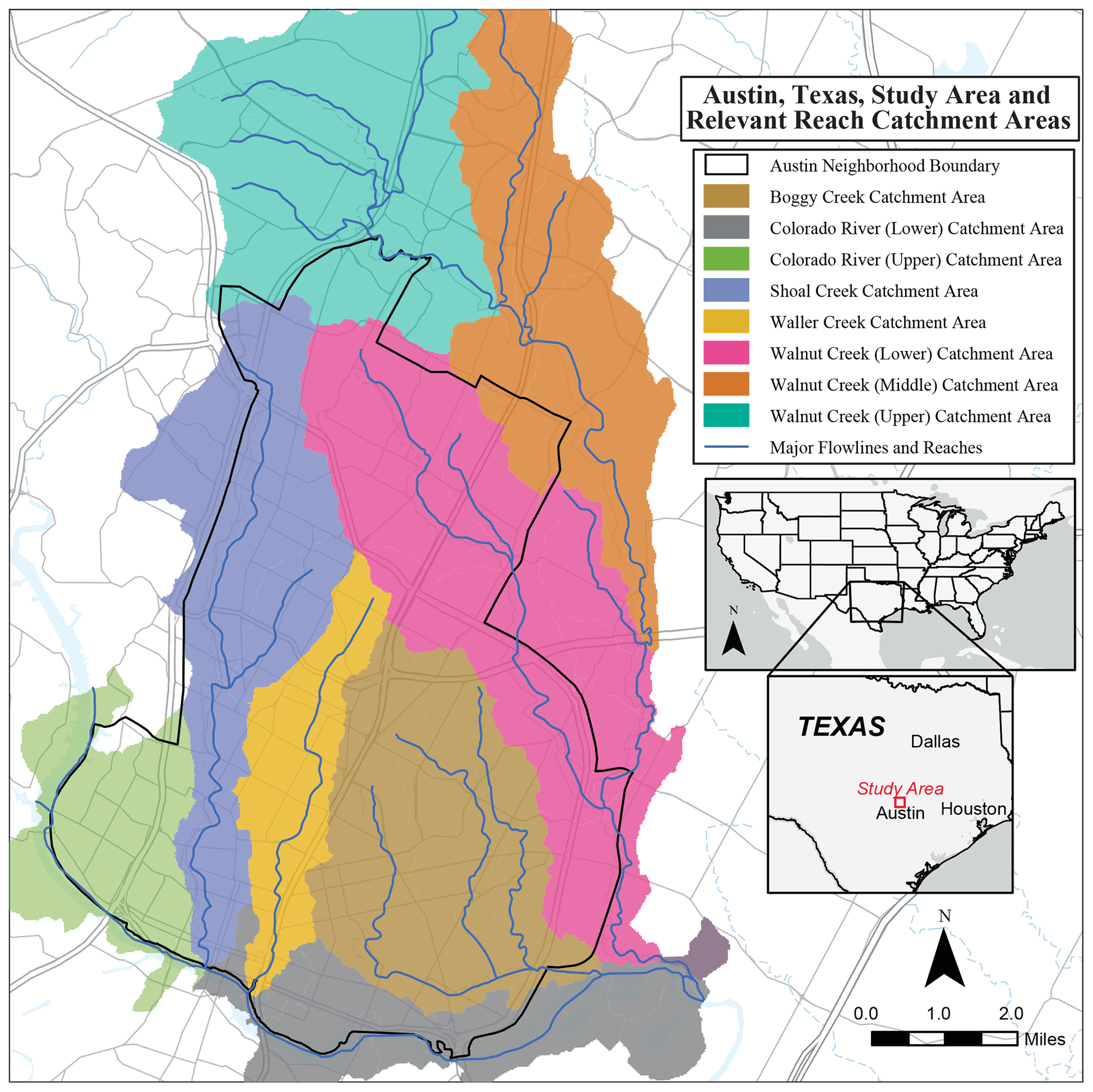
Figure 1Austin, Texas, study area boundary and relevant stream reach catchment areas.
We use the 2015 Memorial Day (25 May 2015) flood in our analysis, as locals refer to this as being the worst flood in recent Austin history. In 2015, Texas saw intense rainfall events from April through May, causing state and local emergency response agencies to be active throughout the entire month of May and the majority of June (Schumann et al., 2016). On Memorial Day, starting at 13:00 Central Standard Time (CST), it began to rain in Austin, TX, pouring 5.2 in. (13.2 cm) in the following 5 h, with 80 % falling within a 2 h period. This value is the second-highest amount of precipitation in a single day in Austin, Texas, since 2002 and the eighth-highest amount since 1927, which is the farthest back that uninterrupted records for this region extend. All stream reaches in this study reached their peak instantaneous flow rates within the 3 h immediately following the end of the precipitation (i.e., by 20:00 CST).
The data sources and tools used in our analysis were deliberately chosen for their broad accessibility across the country, allowing the application of this methodology to occur across the U.S. with little to no data availability concerns (Table 2). Stream reaches, their boundaries, streamflow discharge, and rainfall are all publicly available and provided by the United States Geological Survey (USGS) and the National Oceanic and Atmospheric Administration (NOAA; Table 1). The 1 m DEMs for the contiguous United States are also broadly available from the USGS and through other state and regional agencies. Parcel boundaries are well defined across the country, and while a single national source is not publicly available, most city and state agencies will provide this information for free. For example, the Texas Natural Resources Information System (TNRIS) currently has 228 of 254 counties' parcel data available for free.
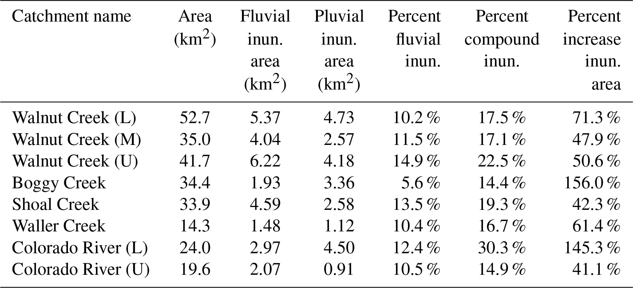
Table 1Austin, Texas, catchment characteristics.
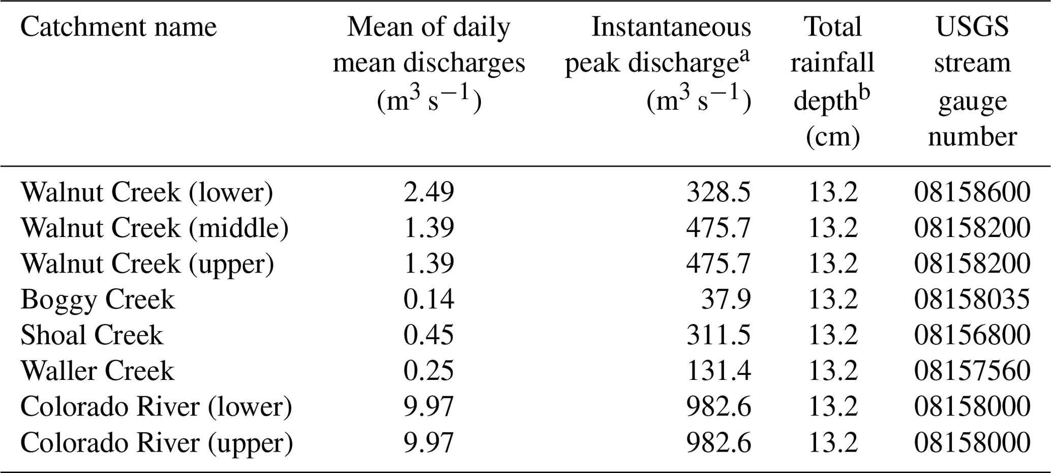
a Peak instantaneous discharge was used as a representation of the worst-case scenario and of the rapid flood characteristics related to the Memorial Day flood. b Total rainfall represents the total amount of precipitation that fell on Memorial Day (25 May 2015) over a 5 h period. Usually, 13.2 cm of rain is approximately a 0.005 annual exceedance probability for this region (according to NOAA historical precipitation data).
Table 2Programming tools and data sources utilized in this methodology.
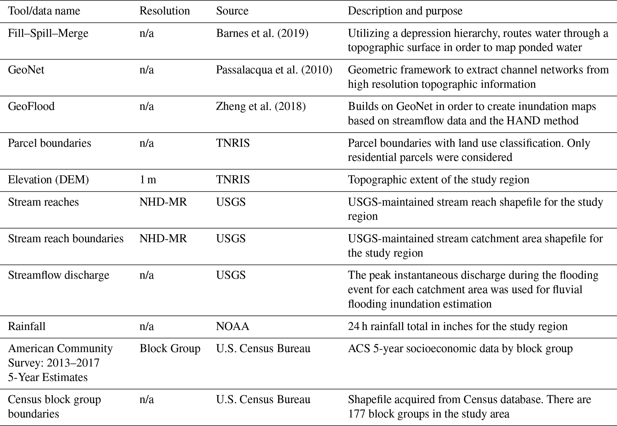
n/a: not applicable. NHD-MR: National Hydrography Dataset Medium Resolution.
The ACS 5-Year Estimates are period estimates that represent data from the previous 60 months, which is the largest sample size when compared to other ACS reports. For example, the 2017 data used in this analysis are an aggregation of data collected from 2013 through 2017. This large sample size is able to dampen outliers and potential errors in sociodemographic data. ACS 5-Year Estimates are available for all block groups across the U.S., which is the highest spatial resolution at which the Census Bureau publishes data, and are therefore able to capture the variation in the demographic make-up of a region. Block groups have a population ranging from 600 to 3000 people, depending on if the block group is in a more rural or urban location.
ACS 5-Year Estimate reports at the block group level are not without disadvantages. Block groups are not perfect delineations of neighborhoods, and can unintentionally group dissimilar neighborhoods (e.g., a predominantly black neighborhood that is grouped with an adjacent predominantly white neighborhood might not capture socioeconomic differences and give a false illusion of neighborhood heterogeneity), creating a large margin of error in some estimations. ACS 5-Year Estimates are also the least current datasets available due to their 5-year look back nature. This 5-year look back period also limits comparisons that can be made between datasets. For example, the 2017 ACS 5-Year Estimate used in this study could not be compared to the 2018 5-Year Estimate, as they would have 4 out of 5 years of overlapping coverage. However, compared to other ACS reports and the difficulties and expenses of other survey data sources, the advantages of using the ACS 5-Year Estimates reports outweigh the disadvantages presented. This analysis uses social and demographic data from the 2017 ACS 5-Year Estimates report, as they best capture the socioeconomic conditions of 2015 (i.e., 2015 is the midpoint of the 2017 dataset). In applications of this methodology in terms of future planning and emergency response, the most relevant 5-Year Estimate will be the one most recently released.
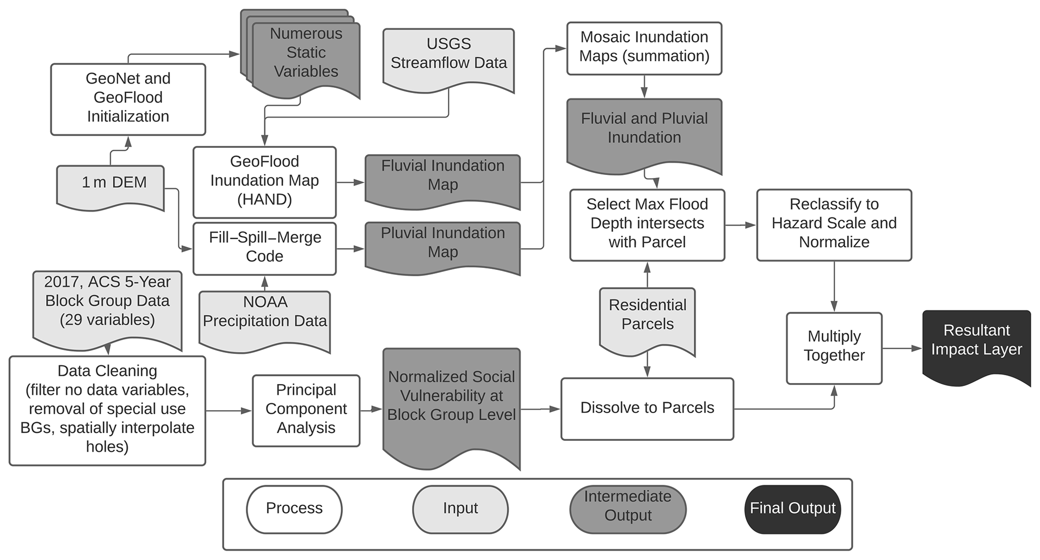
Figure 2Complete workflow of our approach, including fluvial/pluvial inundation estimation and SVI calculation. White boxes indicate a process (mathematical function, program, or action), lightly shaded boxes indicate an outside data input, dark shaded boxes indicate an intermediate dataset, and the black box is the final output/result.
The following subsections detail the methodology and workflow for calculating the flood hazard map, sociodemographic vulnerability, and flood impact index at the parcel level (Fig. 2).
4.1 Flood hazard at the parcel level
The 1 m DEM was first processed using the GeoNet workflow (Passalacqua et al., 2010; Sangireddy et al., 2016). GeoNet extracts channel networks from high-resolution topography data through the application of nonlinear filtering and the identification of geodesic paths as curves of minimum cost. GeoNet uses a Perona–Malik nonlinear smoothing image filter (set to 50 iterations) to remove observational noise and irregularities within the DEM. This nonlinear filter uses gradient information to define the diffusion coefficient in order to preferentially smooth regions outside and within the channel, rather than across its boundary, in order to maintain clear channel boundaries. GeoNet is able to calculate both a geometric and Laplacian curvature based on the desired use. We chose to use the geometric curvature in order to normalize across the entire study region (as compared to the Laplacian calculation, which is more selective). GeoNet uses this information, along with flow accumulation, flow direction, and slope in a cost function representing travel between two points to determine the geodesic curve from the channel head to the basin outlet. GeoFlood integrates terrain and hydrological outputs from GeoNet, which creates, through the application of the Height Above Nearest Drainage (HAND) method, an inundation map (extent and depths of flood waters) along the delineated stream channels for a given input flow rate (Nobre et al., 2011; Zheng et al., 2018).
The HAND method relies on a flow direction raster as one of its primary inputs, thus requiring a hydrologically connected, or a “hydrologically coherent” (Nobre et al., 2011), DEM from which all depressions, pits, and flat areas are removed. Therefore, the resulting estimated fluvial inundation depths do not consider depressions. Given a known centerline water depth, h, at a river segment, the HAND raster is used to produce a water depth grid of the inundated area, F(h), within the local catchment draining to that segment. The water depth, d, at any location, i, is therefore as follows:
The Fill–Spill–Merge algorithm determines the pluvial inundation depths and extents using a uniform runoff depth across the study region. The previous 5 d leading up to the storm event under investigation all recorded some level of precipitation. Furthermore, the storm itself exhibited flash flood characteristics, with 80 % of the precipitation (over 10 cm) falling within 2 h. These conditions led to saturated soils for the majority of downtown Austin, justifying using rainfall depth as an equivalent for runoff depth. We utilized a uniform rainfall depth, as it is a more accurate representation of an input that would be available in a near-real-time scenario as compared to a gridded satellite precipitation measurement. Fill–Spill–Merge routes the rainfall depth through the depression hierarchy to its lowest downstream point before being redistributed to nodes with enough volume to contain the volume of rainwater, with the excess being sent to the “ocean” (Barnes et al., 2019). Fill–Spill–Merge requires an input elevation that is equal to the lowest elevation across the DEM which serves as the ocean or the super-sink of the network that all water not remaining in a depression drains to. To accommodate this, we added an artificial elevation along the entire perimeter of the DEM that was set to 0 ft (0 m). Given a known volume of water in a depression, Vw, and the raster cells within that depression with a known length (l) and width (w), ci=c1, …, cN, the water level in the depression, Zw, is therefore as follows:
with each cell in the depression having a water elevation equal to the computed Zw. For a more detailed explanation of this algorithm, we refer the reader to the Fill–Spill–Merge publication (Barnes et al., 2019) and references therein.
Since the rainfall event lasted approximately 5 h and all stream reaches had their maximum instantaneous streamflows within 3 h following the storm, we chose to use the peak discharge of each reach, independent of time, as a proxy for the worst-case scenario of fluvial flooding. Similarly, we consider the total cumulative rainfall depth as the worst-case scenario for pluvial flooding. The inundation extents produced by GeoFlood and Fill–Spill–Merge and Eqs. (1) and (2) are merged to estimate the compound hazard. Using raster mathematical functions, the fluvial and pluvial inundation estimates are summed. This summation specifically highlights areas that will experience both fluvial and pluvial flooding.
We determine residential parcel hazard by overlaying the inundation and parcel layers and extracting the highest flood depth that intersects each parcel. Numerous factors affect an individual's exposure to a hazard, including, but not limited to, the flood duration, depth of water, velocity of storm water, and water quality (Middelmann-Fernandes, 2010). Therefore, there is uncertainty regarding the direct correlation between flood depth and flood damage (Freni et al., 2010). Regardless, flood depth–damage relations remain one of the leading methodologies for flood exposure estimation in numerous models (de Moel and Aerts, 2011). For this study, flood depth remains the quickest and easiest proxy for hazard.
Adapting methods from other flood communication research, we reclassified flood depths and binned them to a more easily understandable scale that relates water depth to various heights along the average person's body (Calianno et al., 2013; Ahmed et al., 2018a, b). Relating flood depths to human features is becoming a useful tool for relating hazards to physical vulnerability during extreme flood events (Wang and Marsooli, 2021). Putting the hazard in terms of physical vulnerability helps to more easily combine it with social vulnerability in the final impact index. This approach coincides with the United Nations International Strategy for Disaster Reduction (UNISDR), as vulnerability is an assortment of physical and social factors affecting the susceptibility of an individual to the damaging effect of a hazard (ISDR, 2009). Furthermore, this approach avoids the over-/under-inflation of other relative exposure results from one storm to another. For example, if flood depths were only min–max normalized, a small regional flood would appear to have a similar hazard to a large regional flood. Therefore, a household's hazard level refers to the reclassified maximum inundation depth, dmax, at that parcel (Eq. 3).
Before being multiplied by the SVI, the reclassified flood depths are normalized to a 0–1 scale, with 1 having the highest flood hazard and 0 experiencing no flood.
4.2 Sociodemographic vulnerability at the parcel level
We collected sociodemographic vulnerability data at the block group level from Bixler et al. (2021), who utilized data from the 2017 ACS 5-Year Estimates. Bixler et al. (2021)'s procedure is an adaptation of SoVI® specifically developed for Austin, TX, and Texas at large. Of the 29 SoVI® variables, 4 were not available for this time period in Austin at the block group level and were therefore not extracted (e.g., hospitals per capita, percent of population without health insurance, nursing home residents per capita, percent of female-headed households). To further handle missing values, Bixler et al. (2021) excluded special use block groups (e.g., airports, military bases, and prisons) and filled in holes by spatially interpolating from the surrounding area by averaging the values of the neighboring block groups. Min–max scaling all values for each block group further prepared the variables for the principal component analysis (PCA).
Table 3Variables included and excluded from the social vulnerability index (SVI) of Austin, Texas, as retrieved from Bixler et al. (2021).
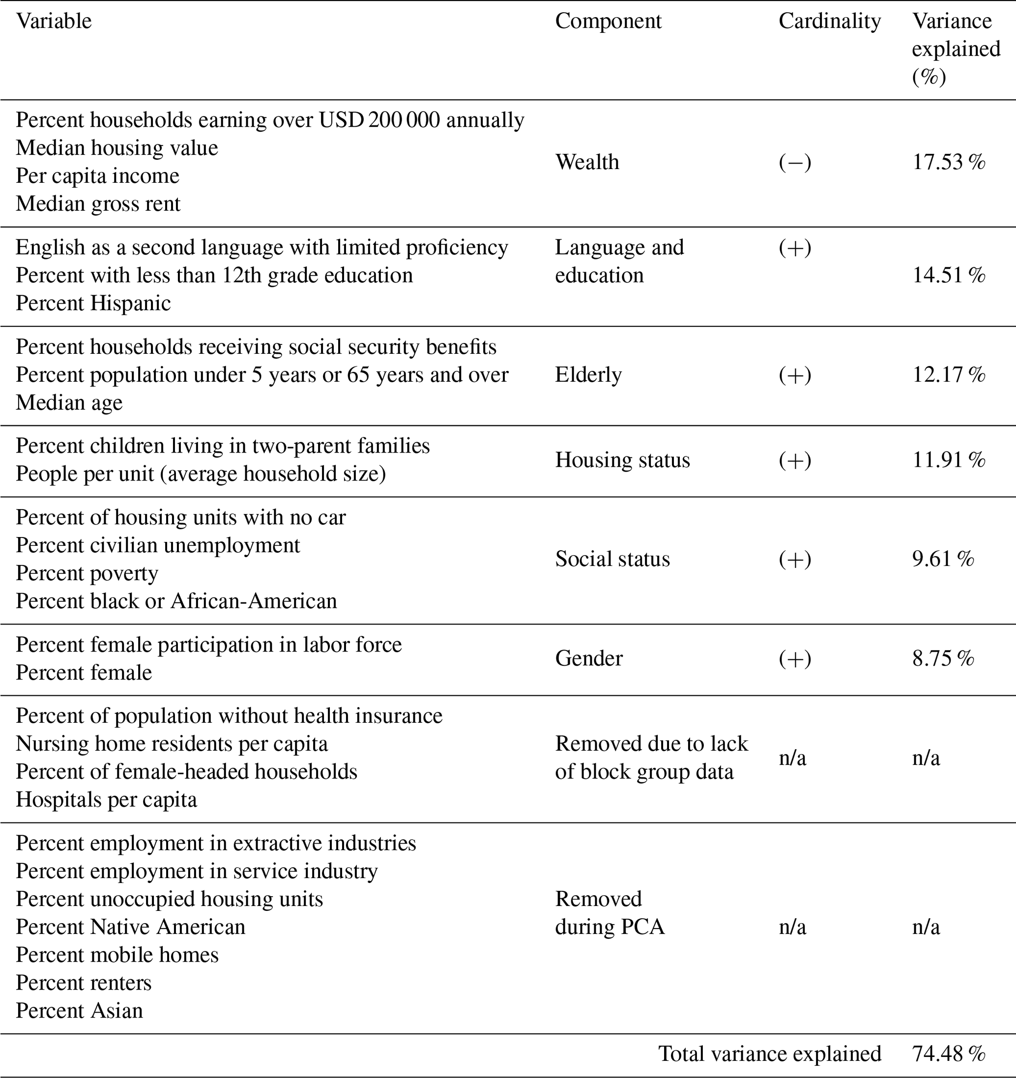
n/a: not applicable.
The PCA's purpose is to reduce the dimensionality to statistically optimized components. A large number of variables are likely to have an influence on an individual's vulnerability. The PCA reduces variables to the most influential factors and merges them into similar highly correlated components. As a result, the PCA eliminated 7 variables, leaving a total of 18 variables divided into six components (wealth, language and education, elderly, housing status, social status, and gender). The 18 variables that remained are therefore the most significant socioeconomic variables (of the original 29) that will impact an individual's social vulnerability (Table 3). The six components are listed in descending order from the highest amount of variance explained. For example, the variables in the wealth component account for 17.53 % of the original variance between all of the variables. The removed variables have less descriptive power and are therefore removed. We manually adjusted the cardinality of each component so that a higher variable value indicated a higher vulnerability (Table 3). For example, wealth has a negative cardinality because having a higher per capita income would make an individual less vulnerable. The numerical composite social vulnerability score for each block group is the sum of the normalized and direction-adjusted values for each variable. This final score was again normalized from 0–1 (with 1 being the most vulnerable). The residential parcel SVI score is the SVI score for the block group to which that parcel belongs.
4.3 Flood impact at the parcel level
As previously described, impact is the product of hazard and vulnerability (Eq. 5). Therefore, household impact is calculated by multiplying the normalized flood hazard value (Eq. 3) by the normalized relative sociodemographic vulnerability value (Eq. 4). Plotted by quintile, the final residential parcel flood impact index highlights the comparative communities that are the least and most impacted.
4.4 Pluvial flooding comparison
GeoFlood has been shown to capture the general fluvial inundation patterns of flood events, with inundation extents overlapping with 60 %–90 % of FEMA inundation extents (Zheng et al., 2018, 2022). To compare Fill–Spill–Merge and our pluvial inundation estimates to a full hydrodynamic model, we employed a physically based 2D hydrodynamic model by using the software ProMaIDes (Protection Measures against Inundation Decision support). ProMaIDes is a modular open-source tool for risk-based assessment for river, urban, and coastal flooding and has been developed at the RWTH Aachen University and Magdeburg-Stendal University of Applied Sciences, Germany (Grimm et al., 2012; Bachmann, 2012, 2021). The hydrodynamic analysis implemented in ProMaIDes is based on a finite volume approach solving the diffusive wave equations, and it includes a multistep backward differentiation method for the temporal discretization (Tsai, 2003).
The 2D model domain for the hydrodynamic model is one subbasin within the Shoal Creek watershed, covering approximately 5 km2. The hydrodynamic model can be driven by spatially and temporally varying rainfall input. However, to enhance comparability, we applied a uniform rainfall depth of 13.2 cm. We used a uniform roughness coefficient for the model area of 0.03 (Manning). To avoid high computational costs, we limited the simulation time to 1 h of rainfall and 5 h of follow-up time, and we downsampled the DEM resolution to 3 m by 3 m cells. The computational time required was 670 min, using an AMD Ryzen 9 3900X 12-core processor. The model's final inundation output was then put through the same reclassification scheme to determine parcel level hazards (Eq. 3). We compared the parcel level hazard values of our terrain-based estimate to the model's final inundation output for all parcels in this subbasin that are not impacted by fluvial flood waters (3015 parcels).
Following the initial preprocessing steps (i.e., initializing GeoNet and GeoFlood), we computed the flood inundation layers (fluvial and pluvial components) in under 28 min on a Linux machine with a 4.2 GHz i5-10210U processor with four cores (eight threads). In the following figures (excluding Fig. 3), inset areas (A) and (B) compare two different locations within Austin, TX, and represent the same area across all figures. Inset (A) to the north highlights an area that is dominated by fluvial flooding. Inset (B) to the south highlights an area that is dominated by pluvial flooding.
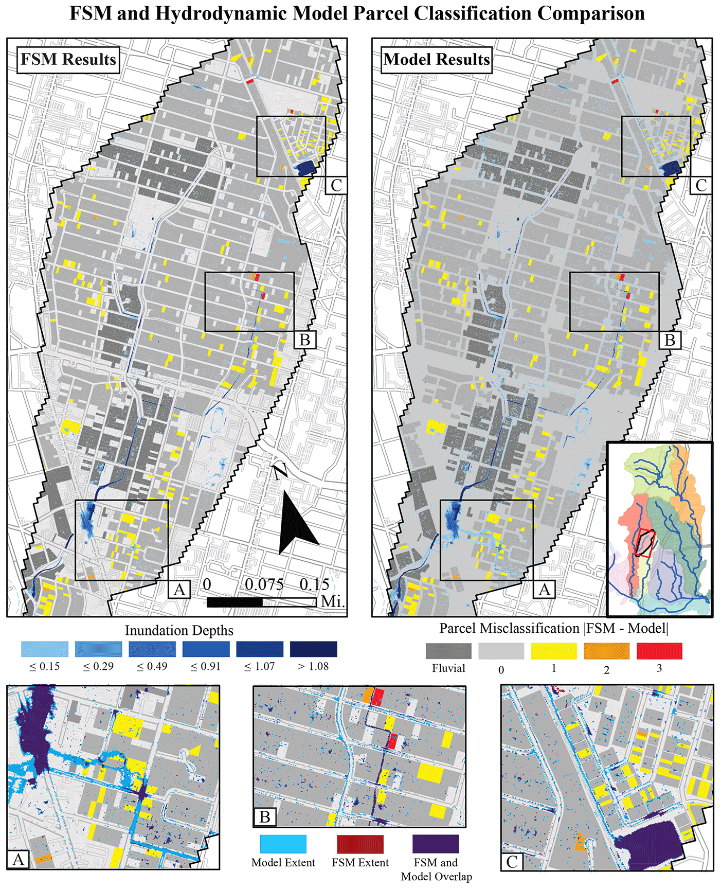
Figure 3Comparison between near real-time estimate (Fill–Spill–Merge) and a 2D physical based hydrodynamic model estimate of pluvial flooding at the parcel level. (a)–(c) highlight areas with concentrated parcel misclassifications. Parcel misclassification is defined as the absolute value of the difference between a parcel's hazard class when determined with either a Fill–Spill–Merge (FSM) or the hydrodynamic model.
5.1 Pluvial flooding comparison
To compare the inundation extent estimates from Fill–Spill–Merge to the physically based model, we overlaid and intersected both rasters (Fig. 3). The intersected raster was then classified into four categories of wet–wet, wet–dry, dry–wet, and dry–dry, with each term in each pair referring to one of the raster layers (i.e., wet–wet refers to a cell that is flooded in both rasters, whereas wet–dry refers to a cell that is flooded in only one raster; Johnson et al., 2019). We define accuracy of the Fill–Spill–Merge model as the number of wet–wet cells divided by the sum of the wet–wet, wet–dry, and dry–wet cells. We found the Fill–Spill–Merge model to be 31 % accurate when excluding any inundated depths less than 1 cm. When the lower limit of allowable depths is increased to 6 cm and 15 cm, the accuracy increases to 44 % and 66.5 % respectively, suggesting that Fill–Spill–Merge performs comparably well at depths that are more likely to affect on the final impact index. Fill–Spill–Merge is predominantly underestimating inundated extents when compared to the model, and this is occurring at larger intersections and along some roadways (Fig. 3; insets A–C).
With the overarching goal to be able to produce a comparable impact map in a fraction of the time, we thus compare reclassified parcel impact maps. Comparing our reclassified parcel level pluvial flood hazard estimates to that of a hydrodynamic model's output, we classified 92 % of the 3015 parcels similarly (Fig. 3). Of the 251 misclassified parcels, 94.4 % (237 parcels) of them were misclassified by only one class (Eq. 3). For example, a residential parcel may have an exposure classification of 2 (between 15 and 29 cm of flooding) in the model output but only a hazard classification of 1 (between 1 and 15 cm of flooding) in the Fill–Spill–Merge estimate. Furthermore, of the misclassified parcels, 69 % (173 parcels) involve a misclassification between no flooding and less than 15 cm of flooding, which is the lowest hazard level. Therefore, the misclassified parcels have a minimal effect on final impact values across the subbasin. Misclassifications are not specifically concentrated in any one area and appear across the subbasin. By reporting the impact at the parcel level and by using hazard classes for flood depths (Eq. 3), we produce comparable impact maps.
5.2 Flood hazard
Through the application of our workflow (Fig. 2) we estimated the worst-case fluvial and pluvial flood extent for the Memorial Day flood (Fig. 4). Insets A1 and B1 show only the fluvial inundation component, while insets A2 and B2 show only the pluvial inundation component of the flood event. The compounding mechanism varies across the study region, with some locations experiencing both fluvial and pluvial flooding in time and space (insets A1 and A2) and other locations compounding only in time (insets B1 and B2).
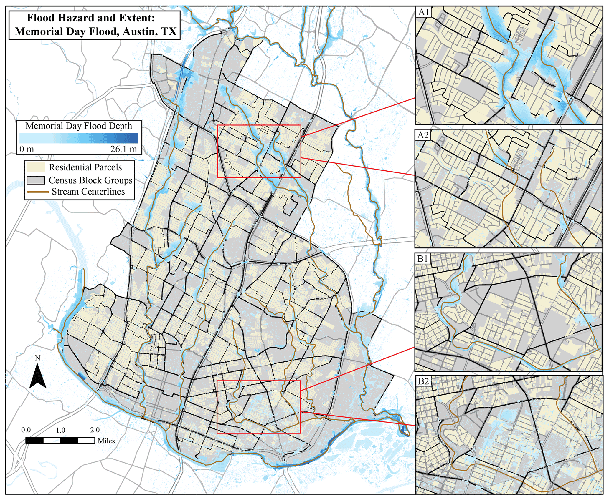
Figure 4Fluvial and pluvial flood depths and extent in Austin, Texas, during the 2015 Memorial Day flood. Insets A1 and B1 show only the fluvial inundation component, while insets A2 and B2 show only the pluvial inundation component of the flood event.
Overall floodwater extents increase when considering both pluvial and fluvial sources (Fig. 5). However, pluvial and fluvial flooding do not affect all locations equally, with some locations being affected more by fluvial flooding and others being affected more by pluvial flooding. Of the 177 block groups within the study area, 67 (37.9 %) experience flooding from only pluvial sources. Flood mapping that exclusively considers fluvial sources would not identify the potential flood hazard of these block groups. Only five block groups have an increase in flood extents greater than 100 %, suggesting that, while pluvial flooding can greatly increase inundation extents across a city or region, fluvial flooding remains the dominant source of flood waters (i.e., the majority of flooding comes from fluvial sources) in those block groups that already experience fluvial flooding. This increase in floodwater extents is also visible by catchment area, showing that the increase in floodwater extents is equally substantial across an entire watershed and not limited to certain locations along a stream reach (Table 4). The increase in floodwater extents within catchment areas, when considering the combined effects of fluvial and pluvial flood sources, ranges from 40 % to 156 %.
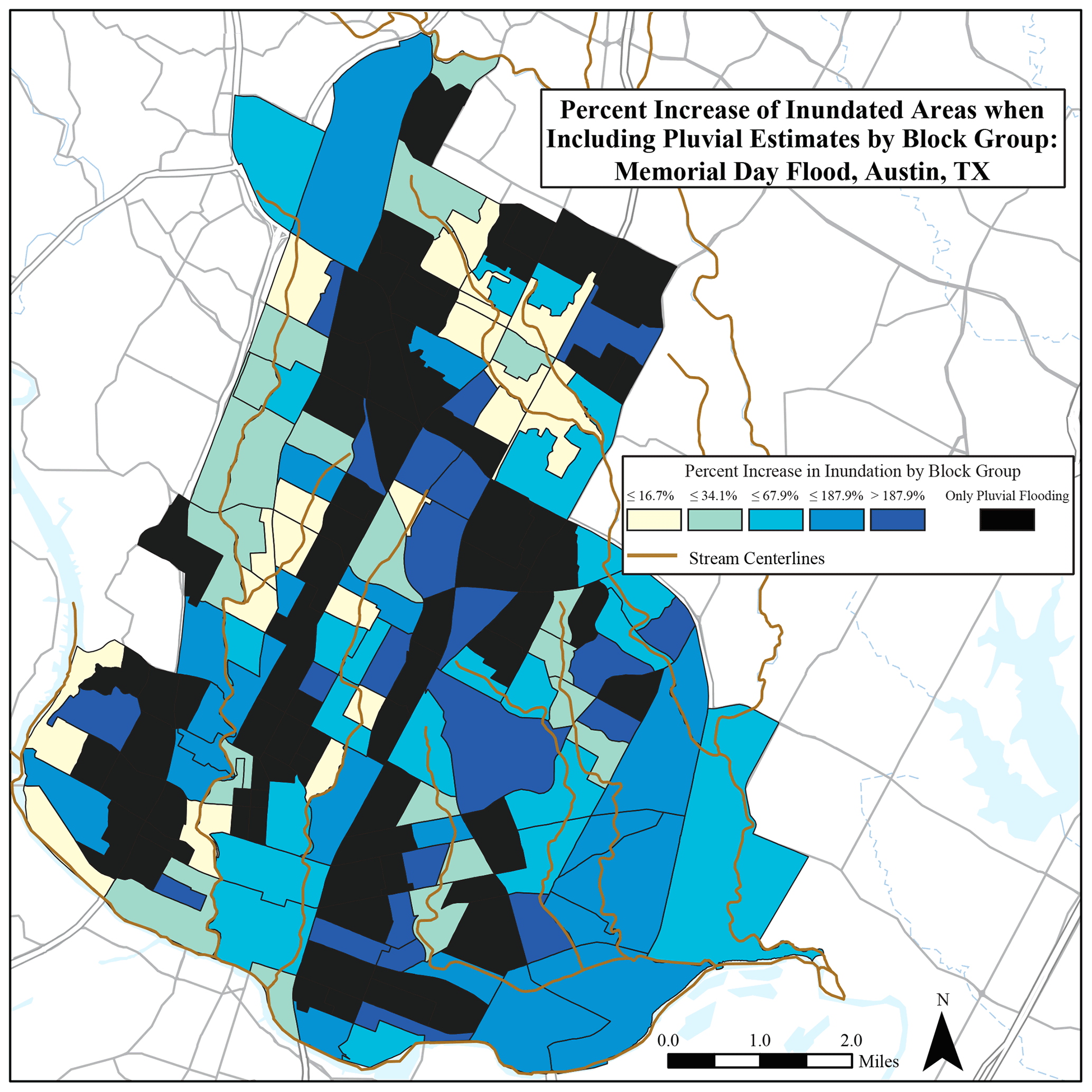
Figure 5Percent increase in inundation extent by census block group when comparing fluvial/pluvial flooding with only fluvial sources during the 2015 Memorial Day flood in Austin, Texas. Darker colors signify a greater percent increase, with black block groups only experiencing pluvial sources.
Table 4Percent increase in inundation extent by catchment area when comparing fluvial/pluvial flooding with only fluvial sources during the 2015 Memorial Day flood in Austin, Texas.
Analyzing flood hazard results by block groups produces a high level of variability, both between and within block groups (Fig. 6). High coefficients of variation (standard deviation divided by mean) signals a wide distribution, suggesting that mean hazard within the giving boundary is going to significantly over- and underestimate household hazard. This is represented in Fig. 6 by the circles, with larger darker circles equating to a higher coefficient of variation. Furthermore, the high dispersion in the average by block group suggests that aggregating at a higher-level boundary (e.g., county) would result in similarly high coefficients of variation.
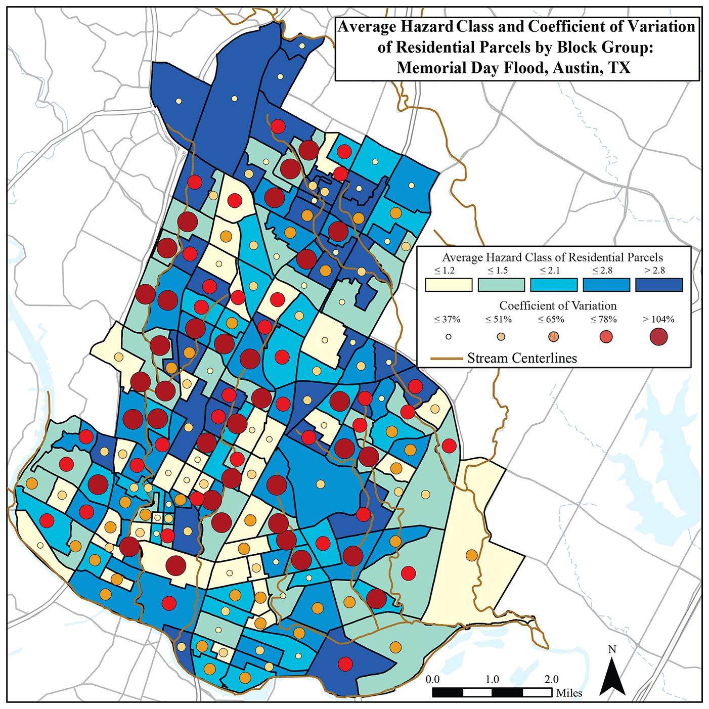
Figure 6Average flood hazard class of residential parcels and their coefficient of variation by census block group during the 2015 Memorial Day flood in Austin, Texas. Darker block groups signify a higher average hazard class, and larger circles signify a higher coefficient of variation.
Reporting hazard values by residential parcels allows for this variability and dispersion to be captured in the final impact calculation (Fig. 7). The reclassification of hazard values (Eq. 3) allows for easier comparisons between regions, thus allowing for quicker identification of potential hot spots. High hazard results predominantly appear along streamlines, which is expected, as fluvial channel floodplains offer more locations for higher depths as compared to topographic depressions which have a much smaller scale in size. Conversely, areas further away from streamlines overwhelmingly appear to be classified in the lowest hazard level and thus are directly impacted, to a lesser extent, by high depth values (Fig. 7).
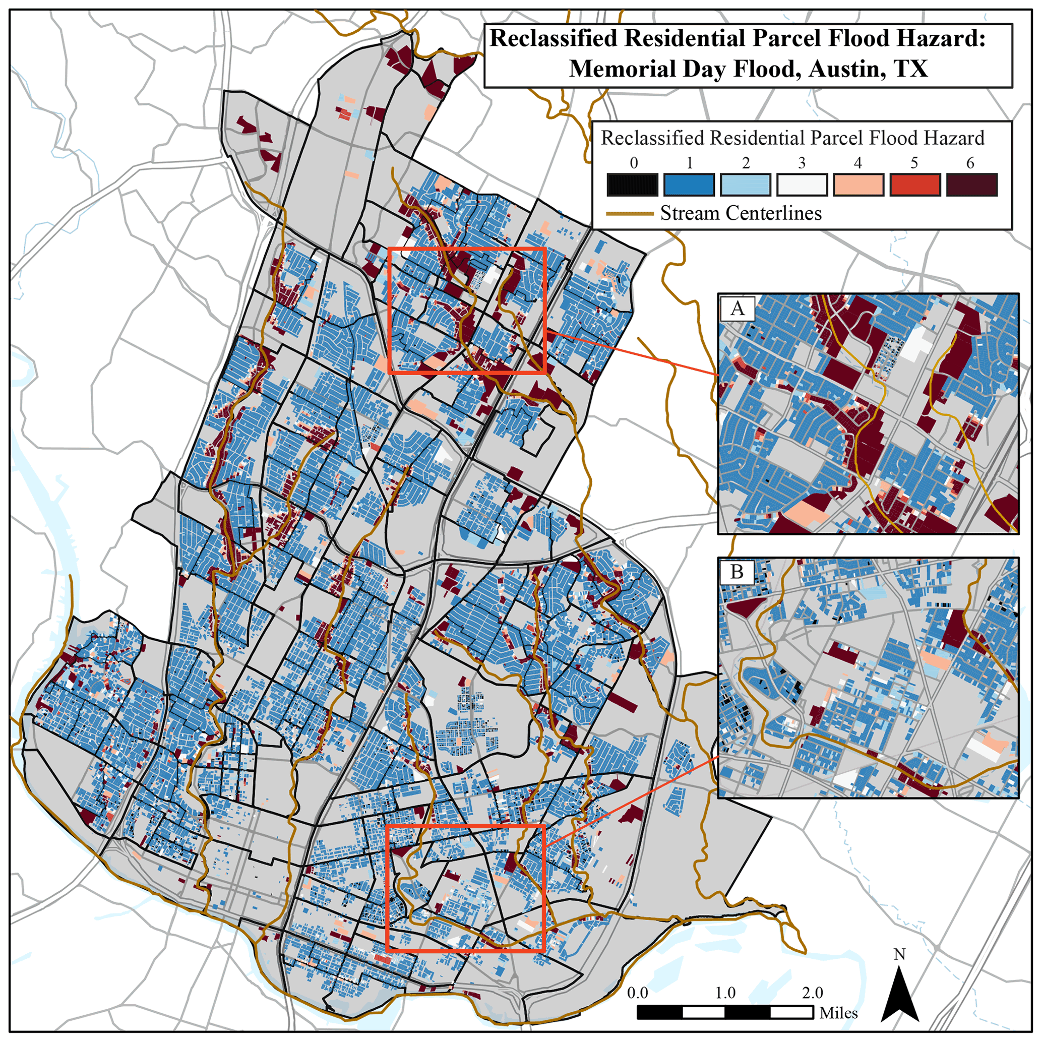
Figure 7Reclassified residential flood hazard during the 2015 Memorial Day flood in Austin, Texas.
5.3 Sociodemographic vulnerability
Clear geographic disparities exist between the eastern and western portions of the study area in terms of the SVI estimates (Fig. 8). Each residential parcel's SVI value is equivalent to the SVI value of the block group that it coincides with. It is important to remember that the SVI estimate shown is relative and is therefore an arbitrary value that can be compared between locations. Parcels with a score of 1 are the most vulnerable, and parcels with a score of 0 are the least vulnerable. The purpose of dissolving the SVI down to the parcel level is to intersect it with our household hazard estimate to compute a parcel specific impact.
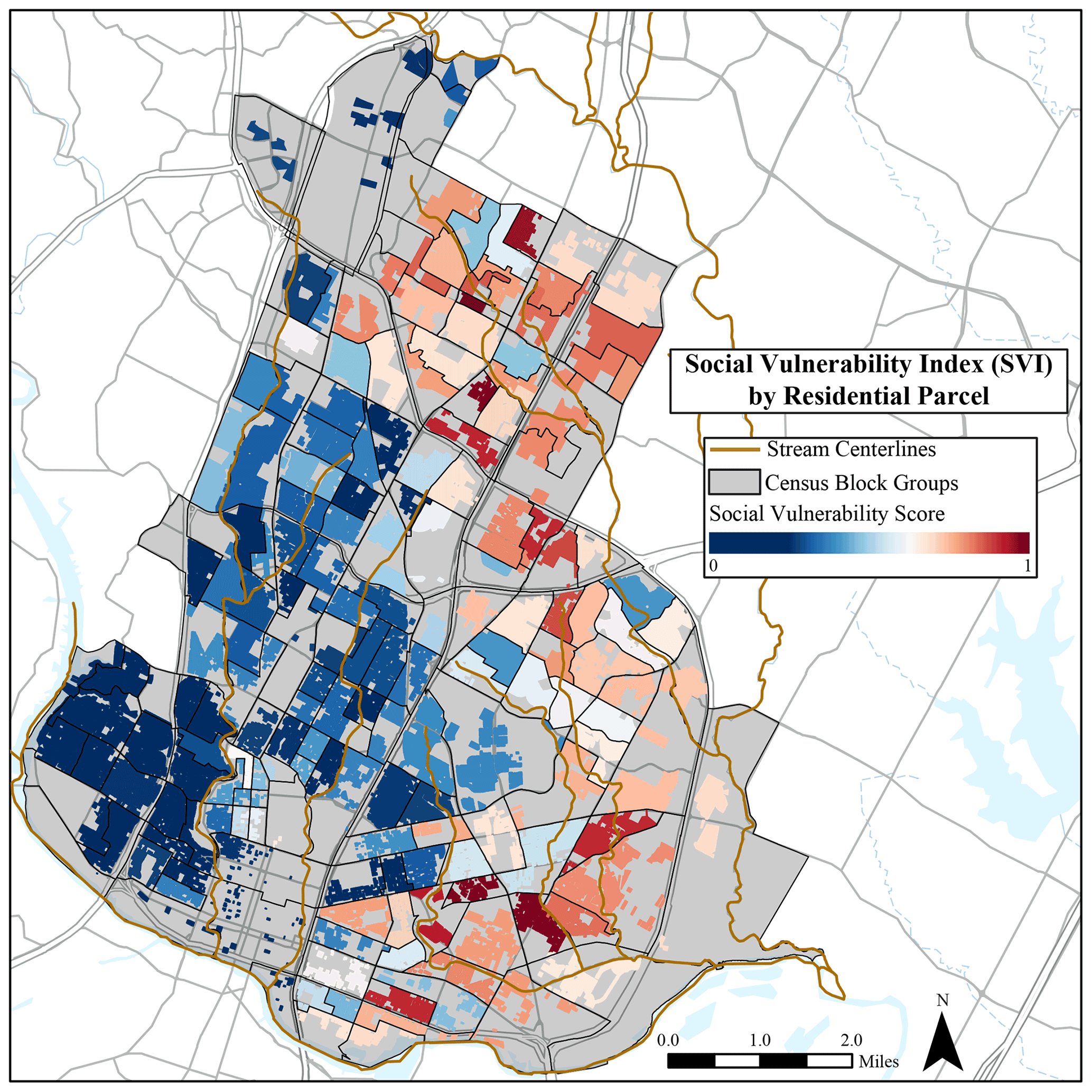
Figure 8Austin, Texas, relative social vulnerability index (SVI), with 1 being most vulnerable and 0 being least vulnerable.
5.4 Impact
There is a clear distinction in the flood impact index between the eastern and western portions of the study area; however, individual block groups themselves also contain variability (Fig. 9). Some locations have varying levels of impact within the same block group, which aggregated estimates would not capture. This is especially prevalent in areas with a higher concentration of higher impact households. Furthermore, high-impact parcels exist in areas not directly adjacent to stream reaches.
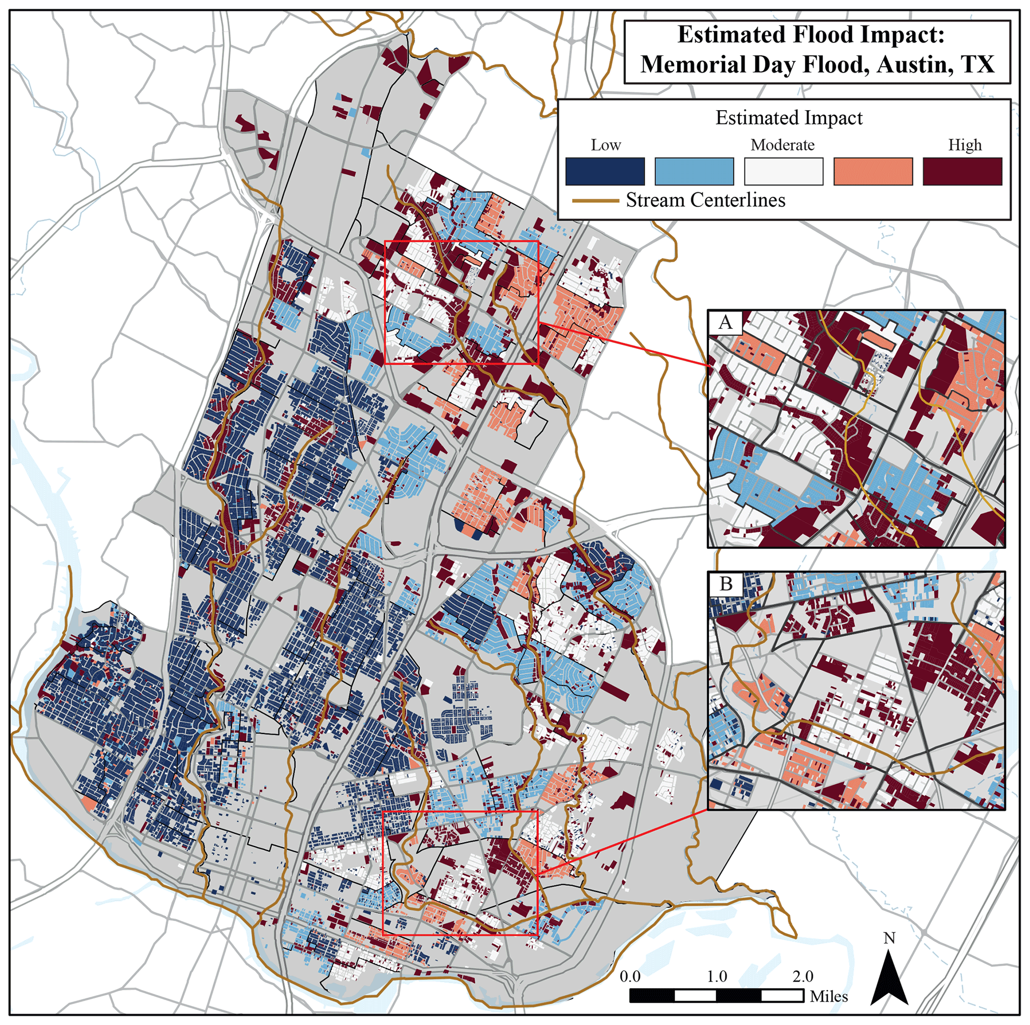
Figure 9Residential flood impact during the 2015 Memorial Day flood in Austin, Texas. Darker reds signify a higher impact, while darker blues signify a lower impact.
6.1 High-resolution compound flooding's role in increasing parcel level hazard
Flood hazard is a function of both inundation extents and depths. Extent determines the breadth of flood waters, with larger flood extents forcing response and recovery efforts to spread out over large areas. Depth determines the level of damage, with a higher depth related to a higher level of damage. A significant source of hazard in urban areas that is often ignored is from pluvial sources (Houston et al., 2011; Grahn and Nyberg, 2017). The exclusion of pluvial flooding from flood mitigation and emergency response planning will result in a drastic under-representation of flood water extents, which could impact millions of households across the United States (Wing et al., 2018). With 38 % of all census block groups in our study area only impacted by pluvial flooding, our results show that pluvial flooding cannot be excluded from flood hazard maps (Fig. 5).
Leading flood hazard maps (e.g., FEMA floodplain maps) and numerous flood risk studies (Burton and Cutter, 2008; Fekete, 2009; Burton, 2010; Finch et al., 2010; Abbas and Routray, 2014; Chakraborty et al., 2014; Tate et al., 2016) do not consider pluvial flood waters in their inundation estimations, instead focusing on fluvial and/or coastal flooding. Recent national level exploratory analyses that do consider pluvial flood waters rely on coarser-resolution (30 m) estimates (Wing et al., 2018; Tate et al., 2021), which can fail to capture small-scale topographic depressions that exist in urban environments. For example, the average width of a four-lane intersection is approximately 15 m. At 30 m resolution, it will not be possible to capture pluvial flooding's impact on roadways. We show that pluvial flooding specifically leads to ponded water on impervious surfaces, such as roadways, intersections, and parking lots, that would otherwise not be identified as being inundated (Fig. 4). Standing water depths greater than 13 cm can be high enough to reach the undercarriage of most passenger cars, inhibiting safe evacuation routes (Moftakhari et al., 2018). Any increase in velocity or depth can block emergency response vehicles from reaching inundated areas.
The co-occurrence of multiple types of flooding will either increase depths (i.e., occurring at the same location), extents (i.e., occurring at the same time), or a combination of both (Wahl et al., 2015). In our study area, compound flooding is predominantly related to increasing extents (Fig. 4). Fluvial flooding is associated with higher depths, concentrated along stream reaches, while pluvial flooding is associated with lower depths spread out over larger areas (Fig. 7). Low depth pluvial flooding can be described as “nuisance flooding”, which has the ability to disrupt transportation networks, impact public safety, and potentially damage property (Moftakhari et al., 2018). Fluvial and pluvial floodwaters require specific mitigation actions; therefore, it is important to quantify this distinction due to the place-based nature of flooding.
The city of Austin's FloodPro software, which is the city's leading source of floodplain information, lacks pluvial flooding information, therefore significantly under-reporting exposure. The inclusion of high-resolution pluvial flooding estimates is necessary for understanding the potential impacts to local infrastructure, residents, and emergency services. High-resolution compound flooding estimates can drastically improve local and regional flood polices' impacts by more accurately addressing flood issues that would otherwise go unnoticed.
6.2 Impact of aggregating hazard and impact to cartographic boundaries
One of the leading purposes of mapping flood hazards with social vulnerability is to identify the most impacted populations and individuals. However, aggregating and reporting estimates to cartographic boundaries can significantly mask household level variability, thus misclassifying some high- and low-impacted households. This misidentification can inhibit the proper allocation of mitigation and emergency response services. Our results show that when household hazard is averaged to census block groups, 60 % of all block groups have a coefficient of variation higher than 50 %, showing that using a central tendency statistic to report flood hazards over a cartographic boundary is not representative of actual flood conditions (Fig. 7).
The majority of recent research on social vulnerability to floods aggregates exposure, hazard, impact, consequence, or the subsequent risk estimates to census tract, zip code, or county boundaries (Burton and Cutter, 2008; Cutter et al., 2013; Chakraborty et al., 2014; Wing et al., 2020; Tate et al., 2021). The two primary reasons for aggregating results are (i) the exploratory nature and large geographic scale of these studies to identify broad regions of interest, and (ii) the aggregated boundary is the resolution of the utilized socioeconomic data. In this study, hazard is heterogeneous within block groups (Fig. 7). Since social vulnerability estimates do not vary within a block group (Fig. 8), the observed heterogeneity in the final impact estimate comes solely from the variability in hazard (Fig. 9). While aggregated results can draw attention to broad regions of risk, household level data are required to properly classify who will be impacted. This is not the first study to incorporate tax parcel data to attempt to estimate a hazard at the household level (Nelson et al., 2015; Fahy et al., 2019); however, previous studies have relied on 100-year floodplain data that lack pluvial estimates. Recent studies have also computed high-resolution compound floodplains based on a multitude of return periods (Bates et al., 2021). However, return period information has implementation limitations in city planning and natural resource management scenarios, as end-users prefer to have information reported in more easily understandable and concrete reference points such as depth values (Luke et al., 2018).
The methodology proposed in this study is not intended to replace large-scale pluvial and compound flood mapping techniques that also utilize high resolution DEMs. As stated in Bermúdez et al. (2018) and Bulti and Abebe (2020a), full hydrodynamic 1D and 2D drainage models are well established to simulate urban pluvial floods and are available in a number of commercial software including SOBEK, XPSWMM 2D, MIKE FLOOD, and InfoWorks ICM (see references therein). Furthermore, Tate et al. (2021) have demonstrated that high-resolution elevation data can be incorporated into full hydrodynamic models at the national scale. While broad exploratory and aggregated studies can assist with equally scaled mitigation and planning programs at the national and state level (e.g., FEMA's National Flood Insurance Program or the Texas Water Development Board's Flood Intended Use Plan), household estimates are necessary for local planning and action plans to effectively serve those who are most impacted. If our final impact estimates were aggregated to the block group level, high-impact households would be masked and not identified. Similarly, low-impact households could be labeled inaccurately, leading to a misappropriation of resources. Highly impacted households are not necessarily limited to high-vulnerability neighborhoods, and it is therefore important to view and report impact and risk estimates in an unbiased manner and at the highest resolution possible. Additionally, this simplified model has fewer input data requirements and requires less technical expertise to produce inundation scenario maps – a feature that is unavailable in full hydrodynamic models.
6.3 Pluvial flooding comparison
While GeoFlood's accuracy and comparability to full hydrodynamic model results has already been researched (Zheng et al., 2018), Fill–Spill–Merge's applicability as a pluvial flooding estimate has not been studied previously. The advantages and disadvantages between a terrain-based estimate of pluvial flooding to a hydrodynamic model can be grouped into two categories, i.e., time and accuracy.
The single subbasin used in the hydrodynamic model, which is 5 km2 in size, represents only 2 % of the entire watershed studied and took over 11 h to compute. This is even when considering the additional model parameters chosen to reduce computational time, such as using a uniform rainfall and roughness coefficient, reduced rainfall and follow up time, and downsampling the DEM. While there is room for the model to be optimized and increase in speed, the terrain-based estimate for the entire study area can be processed in less than 30 min. Rapidly occurring floods (i.e., flooding occurring within 6 h of the onset of precipitation) are some of the most hazardous natural events (Hapuarachchi et al., 2011). Short-term, storm-specific hazard and impact estimates require the speed that comes with our estimation methodology, which can play a critical role in deploying emergency communications before a flooding event begins.
When we compared the terrain-based pluvial inundation estimate to the hydrodynamic model, we found that it had a spatial extent accuracy of 31 %, which further increased to 66.5 % when we ignored the lowest depth classification (Eq. 3). The mismatch in inundation extents predominantly occurred along intersections and roadways, which do not have an impact on our household level classification since these locations do not intersect with residential parcels. This is supported by our 92 % similar household classification, especially considering 237 of the 251 misclassified parcels were by only one class. The difference in the depth estimates of Fill–Spill–Merge and the hydrodynamic model are minimized when we examine maximum parcel depths. Identifying the households with the highest impact is the most important function of the reclassification methodology. In total, 69 % of the misclassified parcels are miscategorized between not experiencing the hazard (i.e., no flooding) and receiving less than 15 cm of flooding (i.e., the lowest classification), therefore having little effect on the final impact calculation.
Comparing simplified conceptual models to full hydrodynamic models is a common methodology for verifying the functionality of the said simplified models in their ability to produce comparable results in a fraction of the time (Lhomme et al., 2008; Bernini and Franchini, 2013; Zheng et al., 2018). A validation of the proposed methodology would involve comparing estimates to historical observations (McGrath et al., 2018). However, these data do not exist for the 2015 Memorial Day flood in Austin, Texas.
6.4 Limitations and future work
There are inherent challenges associated with SVIs and reporting results in terms of relative risk that will require future and more in-depth analyses. Studies have shown that social vulnerability models related to specific hazards and outcomes perform better than generic social vulnerability indices (Tellman et al., 2020). Furthermore, the performance of generic indices has been shown to be statistically biased, based on when the model configuration is manipulated (Tate, 2013). Similarly, while some studies show that flood exposure is higher for socially vulnerable populations (Lee and Jung, 2014; Rolfe et al., 2020), other studies show that socially vulnerable populations can experience the highest exposure to flood hazards, given certain circumstances (Fielding and Burningham, 2005; Bin and Kruse, 2006; Ueland and Warf, 2006; Chakraborty et al., 2014). Resiliency and vulnerability indices are created unequally, and researchers should clearly state index objectives and structure underlying their metrics to support validation of the results based on established goals (Bakkensen et al., 2017). We selected the SoVI® algorithm and variable set due to its widespread adoption and the proof-of-concept nature of our workflow to be able to accept an SVI-like variable.
The simplistic nature of SVIs allows instantaneous estimations, but SVIs cannot measure the full complex nature of vulnerability (Rufat et al., 2015). SVIs could inadvertently weight variables inaccurately (i.e., household income carries the same vulnerability weight as median age), creating a biased depiction of vulnerability over a region, thus misidentifying at-risk individuals and perpetuating risk. SVIs should incorporate city-specific information, including variables such as distance to critical infrastructure (e.g., hospitals) or access to resources (e.g., gas, food, electricity, transportation, and water), to ensure proper representation of all residents. Further consideration needs to be given to estimating social vulnerability at the household level. Census data, especially at the block group level, can have large margins of error. Assuming that values found for the areal units apply at the household level requires a more specific analysis. One such option that has been used to address this concern is the use of primary household survey data (Collins et al., 2015). Despite these limitations, generic social vulnerability indices continue to have prolific use in disaster and emergency research fields and are beneficial in identifying potentially at-risk individuals (Tellman et al., 2020; Tate et al., 2021).
There are also challenges associated with estimating flood hazard. The methods used to estimate exposure are a simplification of much more complex flood mechanics and do not account for variables such as storm drainage networks, movement around buildings and structures, and timing/velocity considerations. One of the known limitations of topographic-based inundation models is that they lack a timing mechanism and can therefore only be used to show a single state of inundation (Bulti and Abebe, 2020b; Fritsch et al., 2016; Lhomme et al., 2008). While this workflow can produce estimates in near-real time, it is important to consider these estimates in the broader context of flood modeling and consider the inherent uncertainties of terrain-based flood mapping. In the context of pluvial flooding, specifically nuisance flooding at lower depths, estimates are directly impacted by DEM accuracy. The DEM used has a vertical accuracy of 6 cm, which is significant when considering flood depths that are between 3 and 10 cm (Moftakhari et al., 2018). While uncertainty and its communication can have a substantial impacts on regulatory and response processes (Downton et al., 2005; Luke et al., 2018), there is also evidence that flood emergency managers are willing to trade larger uncertainties for faster information (McCarthy et al., 2007). As shown, pluvial flooding has a direct impact on roadways and intersections, suggesting that its predominant impact may be in the disruption of traffic and emergency services, especially considering the exponential decrease in vehicular traffic as a result of standing water and the complete halting of traffic when depths exceed 15 cm (Pregnolato et al., 2017). Furthermore, initial conditions, and whether or not there is a base amount of ponded water, can be considered and applied to this methodology as well by routing a volume/depth through the topography before any additional runoff is routed.
There are other topographic-based inundation methods that incorporate more flooding factors such as land use information factors, including infiltration and friction (Chu et al., 2013b; Appels et al., 2011; Antoine et al., 2009; Lhomme et al., 2008). However, it is important to note the increased computational time involved with such methods. For example, the rapid flood spreading model (RFSM) only requires an input flood volume, elevation, and surface roughness (Bernini and Franchini, 2013; Lhomme et al., 2008). Due to the inclusion of surface roughness, the RFSM method is approximately 3.8 times slower than the Fill–Spill–Merge method utilized on our study (calculated by comparing the ratio of DEM cells to computational time in our study to theirs, with 502 ×106 cells in 28 min with our method and 387 000 cells in 5 s with theirs). In a near-real time scenario when the entire storm event occurs in less than 5 h, the difference between a computational time of 28 min (our computational time) and 106 min (our computational time multiplied by 3.8, which is the estimated speed ratio of RFSM to Fill–Spill–Merge) is substantial. Future research will examine how to improve FSM's ability to estimate lower depth inundation extents (i.e., less than 15 cm) and how road network disruptions impact a household's ability to access critical resources in near-real time (grocery stores, gas stations, pharmacies, hospitals, etc.)
While it is necessary to understand both short-term and long-term risk, as they require unique actions and policies to address them, this study is a specific attempt to identify short-term impacts for a known storm event. Long-term future flood risks caused by the projected increase in the frequency of extreme weather events due to climate change will require additional analyses. Future flood risk calculations can incorporate this workflow by using modeled storm characteristics and projected sociodemographic information. As a supplemental tool, this workflow can contribute to other research, response, and mitigation efforts.
The proposed workflow in this study creates a storm-specific urban flood impact index at the parcel level using high-resolution topographic data, near-real-time pluvial and fluvial flood estimations, and a region-specific social vulnerability index. The application of this workflow to the Memorial Day flood in Austin, TX, showed that estimating fluvial flooding alone is not enough to predict urban flood hazards. We showed that our pluvial hazard estimate can accurately determine the parcel level impact index 94.4 % of the time, when compared to a full hydrodynamic model, in near-real time. Furthermore, we show that aggregating results to cartographic boundaries masks the dispersion of hazards and impacts, thus making it difficult to identify priority locations that must be addressed in planning, management, and emergency response scenarios. Through the inclusion of a social vulnerability index, end-users are better informed in identifying those individuals facing the greatest impact (a product of flood hazard and vulnerability).
This methodology's power lies in the ability to calculate a 1 m horizontal resolution inundation estimate for large urban areas (>250 km2) in under 30 min on a personal computer while strictly using open-source data that are theoretically available for the entire United States (i.e., census data, USGS stream gauge data, rainfall data, DEMs, and residential parcels can generally be found free online for the majority of the country). Therefore, this framework can estimate a region- and storm-specific impact index in near-real time, anywhere, with widely available computing resources. Future work will explore more, including more flooding and vulnerability factors, such as non-census sociodemographic data, social and governance networks, coastal compound flooding, and local infrastructure data to improve impact estimates.
All data used in this analysis are publicly obtained from their respective sources, including NOAA, USGS, TNRIS, and the U.S. Census Bureau. The GeoFlood and Fill–Spill–Merge codes can be found on their respective GitHub pages (https://github.com/r-barnes/Barnes2020-FillSpillMerge, Barnes, 2022; https://github.com/passaH2O/GeoFlood, , ). All data and the associated codes used can be retrieved from https://doi.org/10.5281/zenodo.6584401 (Preisser et al., 2022).
PP and RPB supervised MP during the entire research process, assisting with the conceptualization and the development of the methodology of the presented research. MP conducted the data collection, investigation, and analysis that make up the presented research. JH created the hydrodynamic comparison datasets that MP utilized in the analysis. MP wrote the original draft and created the visualizations of the paper, with all co-authors contributing to reviewing and editing subsequent drafts.
The contact author has declared that none of the authors has any competing interests.
Publisher's note: Copernicus Publications remains neutral with regard to jurisdictional claims in published maps and institutional affiliations.
We thank the reviewers and editor for providing valuable comments that have improved the clarity and contents of this paper.
This material is based upon work supported by the National Science Foundation Graduate Research Fellowship (grant no. DGE-1610403), the NOAA-JTTI Program (grant no. NA19OAR4590229), and Planet Texas 2050, a research grand challenge at the University of Texas at Austin.
This paper was edited by Hongkai Gao and reviewed by two anonymous referees.
Abbas, H. B. and Routray, J. K.: Vulnerability to flood-induced public health risks in Sudan, Disast. Prevent. Manage., 23, 395–419, https://doi.org/10.1108/DPM-07-2013-0112, 2014. a
Agard, J. and Schipper, E. L. F.: Glossary, Annex II, in: Managing the Risks of Extreme Events and Disasters to Advance Climate Change Adaptation: Special Report of the Intergovernmental Panel on Climate Change, edited by: Birkmann, J., Campos, M., Dubeux, C., Nojiri, Y., Olsson, L., Osman-Elasha, B., Pelling, M., Prather, M., Rivera-Ferre, M., Ruppel, O., Sallenger, A., Smith, K., and St. Clair, A., Cambridge Univesrity Press, Cambridge, UK, and New York, NY, USA, 1757–1776, https://doi.org/10.1016/s0959-3780(06)00031-8, 2012. a
Ahmed, F., Khan, M. S. A., Warner, J., Moors, E., and Terwisscha Van Scheltinga, C.: Integrated Adaptation Tipping Points (IATPs) for urban flood resilience, Environ. Urbaniz., 30, 575–596, https://doi.org/10.1177/0956247818776510, 2018a. a
Ahmed, F., Moors, E., Khan, M. S. A., Warner, J., and Terwisscha van Scheltinga, C.: Tipping points in adaptation to urban flooding under climate change and urban growth: The case of the Dhaka megacity, Land Use Policy, 79, 496–506, https://doi.org/10.1016/j.landusepol.2018.05.051, 2018b. a
Antoine, M., Javaux, M., and Bielders, C.: What indicators can capture runoff-relevant connectivity properties of the micro-topography at the plot scale?, Adv. Water Resour., 32, 1297–1310, https://doi.org/10.1016/j.advwatres.2009.05.006, 2009. a
Appels, W. M., Bogaart, P. W., and van der Zee, S. E.: Influence of spatial variations of microtopography and infiltration on surface runoff and field scale hydrological connectivity, Adv. in Water Resour., 34, 303–313, https://doi.org/10.1016/j.advwatres.2010.12.003, 2011. a
Bachmann, D.: Beitrag zur Entwicklung eines Entscheidungsunterstützungssystems zur Bewertung und Planung von Hochwasserschutzmaßnahmen, PhD thesis, Institut für Wasserbau und Wasserwirtschaft, RWTH Aachen, Aachen, https://d-nb.info/1023005069/34 (last access: 15 March 2022), 2012. a
Bachmann, D.: ProMaIDes: State-of-the Science Flood Risk Management Tool, https://promaides.h2.de/promaides/ (last access: 15 March 2022), 2021. a
Bakkensen, L. A., Fox-Lent, C., Read, L. K., and Linkov, I.: Validating Resilience and Vulnerability Indices in the Context of Natural Disasters, Risk Anal., 37, 982–1004, https://doi.org/10.1111/risa.12677, 2017. a
Barnes, R.: r-barnes/Barnes2020-FillSpillMerge, GitHub [code], https://github.com/r-barnes/Barnes2020-FillSpillMerge, last access: 28 July 2022. a
Barnes, R., Callaghan, K., and Wickert, A.: Computing water flow through complex landscapes – Part 3: Fill-Spill-Merge: Flow routing in depression hierarchies, Earth Surf. Dynam., 7, 737–753, https://doi.org/10.5194/esurf-7-737-2019, 2019. a, b, c, d, e, f
Barnes, R., Callaghan, K. L., and Wickert, A. D.: Computing water flow through complex landscapes – Part 2: Finding hierarchies in depressions and morphological segmentations, Earth Surf. Dynam., 8, 431–445, https://doi.org/10.5194/esurf-8-431-2020, 2020. a
Bates, P. D., Quinn, N., Sampson, C., Smith, A., Wing, O., Sosa, J., Savage, J., Olcese, G., Neal, J., Schumann, G., Giustarini, L., Coxon, G., Porter, J. R., Amodeo, M. F., Chu, Z., Lewis-Gruss, S., Freeman, N. B., Houser, T., Delgado, M., Hamidi, A., Bolliger, I., McCusker, K., Emanuel, K., Ferreira, C. M., Khalid, A., Haigh, I. D., Couasnon, A., Kopp, R., Hsiang, S., and Krajewski, W. F.: Combined Modeling of US Fluvial, Pluvial, and Coastal Flood Hazard Under Current and Future Climates, Water Resour. Res., 57, 1–29, https://doi.org/10.1029/2020WR028673, 2021. a, b, c
Bermúdez, M., Ntegeka, V., Wolfs, V., and Willems, P.: Development and Comparison of Two Fast Surrogate Models for Urban Pluvial Flood Simulations, Water Resour. Manage., 32, 2801–2815, https://doi.org/10.1007/s11269-018-1959-8, 2018. a
Bernini, A. and Franchini, M.: A Rapid Model for Delimiting Flooded Areas, Water Resour. Manage., 27, 3825–3846, https://doi.org/10.1007/s11269-013-0383-3, 2013. a, b
Bin, O. and Kruse, J. B.: Real Estate Market Response to Coastal Flood Hazards, Nat. Hazards Rev., 7, 137–144, https://doi.org/10.1061/(asce)1527-6988(2006)7:4(137), 2006. a
Bixler, R. P., Yang, E., Richter, S. M., and Coudert, M.: Boundary crossing for urban community resilience: A social vulnerability and multi-hazard approach in Austin, Texas, USA, Int. J. Disast. Risk Reduct., 66, 102613, https://doi.org/10.1016/j.ijdrr.2021.102613, 2021. a, b, c, d
Bulti, D. T. and Abebe, B. G.: A review of flood modeling methods for urban pluvial flood application, Model. Earth Syst. Environ., 6, 1293–1302, https://doi.org/10.1007/s40808-020-00803-z, 2020a. a
Bulti, D. T. and Abebe, B. G.: A review of flood modeling methods for urban pluvial flood application, Model. Earth Syst. Environ., 6, 1293–1302, https://doi.org/10.1007/s40808-020-00803-z, 2020b. a
Burton, C. and Cutter, S. L.: Levee Failures and Social Vulnerability in the Sacramento-San Joaquin Delta Area, California, Nat. Hazards Rev., 9, 136–149, https://doi.org/10.1061/(asce)1527-6988(2008)9:3(136), 2008. a, b
Burton, C. G.: Social Vulnerability and Hurricane Impact Modeling, Nat. Hazards Rev., 11, 58–68, https://doi.org/10.1061/(asce)1527-6988(2010)11:2(58), 2010. a
Calianno, M., Ruin, I., and Gourley, J. J.: Supplementing flash flood reports with impact classifications, J. Hydrol., 477, 1–16, https://doi.org/10.1016/j.jhydrol.2012.09.036, 2013. a
Callaghan, K. L. and Wickert, A. D.: Computing water flow through complex landscapes – Part 1: Incorporating depressions in flow routing using FlowFill, Earth Surf. Dynam., 7, 737–753, https://doi.org/10.5194/esurf-7-737-2019, 2019. a, b
Cardona, O. D., Van Aalst, M. K., Birkmann, J., Fordham, M., Mc Gregor, G., Rosa, P., Pulwarty, R. S., Schipper, E. L. F., Sinh, B. T., Décamps, H., Keim, M., Davis, I., Ebi, K. L., Lavell, A., Mechler, R., Murray, V., Pelling, M., Pohl, J., Smith, A. O., and Thomalla, F.: Determinants of risk: Exposure and vulnerability, in: Managing the Risks of Extreme Events and Disasters to Advance Climate Change Adaptation: Special Report of the Intergovernmental Panel on Climate Change, Cambridge Univesrity Press, Cambridge, UK, and New York, NY, USA, 65–108, https://doi.org/10.1017/CBO9781139177245.005, 2012. a, b, c, d
Chakraborty, J., Collins, T. W., Montgomery, M. C., and Grineski, S. E.: Social and Spatial Inequities in Exposure to Flood Risk in Miami, Florida, Nat. Hazards Rev., 15, 04014006, https://doi.org/10.1061/(asce)nh.1527-6996.0000140, 2014. a, b, c, d
Chu, X., Yang, J., Chi, Y., and Zhang, J.: Dynamic puddle delineation and modeling of puddle-to-puddle filling-spilling-merging-splitting overland flow processes, Water Resour. Res., 49, 3825–3829, https://doi.org/10.1002/wrcr.20286, 2013a. a, b
Chu, X., Yang, J., Chi, Y., and Zhang, J.: Dynamic puddle delineation and modeling of puddle-to-puddle filling-spilling-merging-splitting overland flow processes, Water Resour. Res., 49, 3825–3829, https://doi.org/10.1002/wrcr.20286, 2013b. a
Collins, T. W., Grineski, S. E., Chakraborty, J., Montgomery, M. C., and Hernandez, M.: Downscaling Environmental Justice Analysis: Determinants of Household-Level Hazardous Air Pollutant Exposure in Greater Houston, Ann. Assoc. Am. Geogr., 105, 684–703, https://doi.org/10.1080/00045608.2015.1050754, 2015. a
Collins, T. W., Grineski, S. E., Chakraborty, J., and Flores, A. B.: Environmental injustice and Hurricane Harvey: A household-level study of socially disparate flood exposures in Greater Houston, Texas, USA, Environ. Res., 179, 108772, https://doi.org/10.1016/j.envres.2019.108772, 2019. a
Cutter, S. L., Boruff, B., and Shirley, W. L.: Social vulnerability to environmental hazards, Social Sci. Quart., 84, 242–261, https://doi.org/10.1111/1540-6237.8402002, 2003. a, b
Cutter, S. L., Emrich, C. T., Morath, D. P., and Dunning, C. M.: Integrating social vulnerability into federal flood risk management planning, J. Flood Risk Manage., 6, 332–344, https://doi.org/10.1111/jfr3.12018, 2013. a, b
de Carvalho Júnior, O. A., Guimarães, R. F., Montgomery, D. R., Gillespie, A. R., Gomes, R. A. T., Martins, É. D. S., and Silva, N. C.: Karst depression detection using ASTER, ALOS/PRISM and SRTM-derived digital elevation models in the Bambuí group, Brazil, Remote Sens., 6, 330–351, https://doi.org/10.3390/rs6010330, 2013. a
de Moel, H. and Aerts, J. C.: Effect of uncertainty in land use, damage models and inundation depth on flood damage estimates, Nat. Hazards, 58, 407–425, https://doi.org/10.1007/s11069-010-9675-6, 2011. a
Downton, M. W., Morss, R. E., Wilhelmi, O. V., Gruntfest, E., and Higgins, M. L.: Interactions between scientific uncertainty and flood management decisions: Two case studies in Colorado, Environ. Hazards, 6, 134–146, https://doi.org/10.1016/j.hazards.2006.05.003, 2005. a
Fahy, B., Brenneman, E., Chang, H., and Shandas, V.: Spatial analysis of urban flooding and extreme heat hazard potential in Portland, OR, Int. J. Disast. Risk Reduct., 39, 101117, https://doi.org/10.1016/j.ijdrr.2019.101117, 2019. a
Falconer, R. H., Cobby, D., Smyth, P., Astle, G., Dent, J., and Golding, B.: Pluvial flooding: New approaches in flood warning, mapping and risk management, J. Flood Risk Manage., 2, 198–208, https://doi.org/10.1111/j.1753-318X.2009.01034.x, 2009. a
Fekete, A.: Validation of a social vulnerability index in context to river-floods in Germany, Nat. Hazards Earth Syst. Sci., 9, 393–403, https://doi.org/10.5194/nhess-9-393-2009, 2009. a
Fielding, J. and Burningham, K.: Environmental inequality and flood hazard, Local Environ., 10, 379–395, https://doi.org/10.1080/13549830500160875, 2005. a
Finch, C., Emrich, C. T., and Cutter, S. L.: Disaster disparities and differential recovery in New Orleans, Populat. Environ., 31, 179–202, https://doi.org/10.1007/s11111-009-0099-8, 2010. a
Flanagan, B. E., Gregory, E. W., Hallisey, E. J., Heitgerd, J. L., and Lewis, B.: A Social Vulnerability Index for Disaster Management, J. Homeland Secur. Emerg. Manage., 8, 1–22, https://doi.org/10.2202/1547-7355.1792, 2011. a
Freni, G., La Loggia, G., and Notaro, V.: Uncertainty in urban flood damage assessment due to urban drainage modelling and depth-damage curve estimation, Water Sci. Technol., 61, 2979–2993, https://doi.org/10.2166/wst.2010.177, 2010. a
Fritsch, K., Assmann, A., and Tyrna, B.: Long-term experiences with pluvial flood risk management, in: E3S Web of Conferences, 7, https://doi.org/10.1051/e3sconf/20160704017, 2016. a
Grahn, T. and Nyberg, L.: Assessment of pluvial flood exposure and vulnerability of residential areas, Int. J. Disast. Risk Reduct., 21, 367–375, https://doi.org/10.1016/j.ijdrr.2017.01.016, 2017. a
Grimm, C., Wöffler, T., Bachmann, D., and Schüttrumpf, H.: Risk management in coastal engineering: Applied coastal research projects for Northern Germany, Wasser Abfall, 14, 53–55, 2012. a
Guo, K., Guan, M., and Yu, D.: Urban surface water flood modelling – a comprehensive review of current models and future challenges, Hydrol. Earth Syst. Sci., 25, 2843–2860, https://doi.org/10.5194/hess-25-2843-2021, 2021. a
Hapuarachchi, H. A. P., Wang, Q. J., and Pagano, T. C.: A review of advances in flash flood forecasting, Hydrol. Process., 2784, 2771–2784, https://doi.org/10.1002/hyp.8040, 2011. a
Houston, D., Werrity, A., Bassett, D., Geddes, A., Hoolachan, A., and McMillan, M.: Pluvial(rain-related) flooding in urban areas: the invisible hazard, Joseph Rowntree Foundation, https://www.jrf.org.uk/report/pluvial-rain-related-flooding-urban-areas-invisible-hazard#jl_downloads_0 (last access: 15 March 2022), 2011. a
ISDR: UNISDR Terminology on Disaster Risk, Tech. rep., ISDR, https://doi.org/10.7591/9781501701498-008, 2009. a, b
Jenson, S. K. and Domingue, J. O.: Extracting topographic structure from digital elevation data for geographic information system analysis, Photogram. Eng. Remote Sens., 54, 1593–1600, 1988. a
Johnson, M. J., Munasinghe, D., Eyelade, D., and Cohen, S.: An integrated evaluation of the National Water Model (NWM)–Height above nearest drainage (HAND) flood mapping methodology, Nat. Hazards Earth Syst. Sci., 19, 2405–2420, https://doi.org/10.5194/nhess-19-2405-2019, 2019. a
Kaźmierczak, A. and Cavan, G.: Surface water flooding risk to urban communities: Analysis of vulnerability, hazard and exposure, Landsc. Urban Plan., 103, 185–197, https://doi.org/10.1016/j.landurbplan.2011.07.008, 2011. a
Kron, W.: Flood risk = hazard ⋅ values ⋅ vulnerability, Water Int., 30, 58–68, https://doi.org/10.1080/02508060508691837, 2005. a
Le, P. V. V. and Kumar, P.: Power law scaling of topographic depressions and their hydrologic connectivity, Geophys. Res. Lett., 41, 1553–1559, https://doi.org/10.1002/2013GL059114, 2014. a
Lee, D. and Jung, J.: The growth of low-income population in floodplains: A case study of Austin, TX, KSCE J. Civ. Eng., 18, 683–693, https://doi.org/10.1007/s12205-014-0205-z, 2014. a
Lewin, J. and Ashworth, P. J.: The negative relief of large river floodplains, Earth-Sci. Rev., 129, 1–23, https://doi.org/10.1016/j.earscirev.2013.10.014, 2014. a
Lhomme, J., Sayers, P., Gouldby, B., Wills, M., and Mulet-Marti, J.: Recent development and application of a rapid flood spreading method, in: Flood Risk Management: Research and Practice, Taylor & Francis Group, 15–24, ISBN 9780429207129, 2008. a, b, c, d
Li, S., MacMillan, R. A., Lobb, D. A., McConkey, B. G., Moulin, A., and Fraser, W. R.: Lidar DEM error analyses and topographic depression identification in a hummocky landscape in the prairie region of Canada, Geomorphology, 129, 263–275, https://doi.org/10.1016/j.geomorph.2011.02.020, 2011. a
Lindsay, J. B. and Creed, I. F.: Removal of artifact depressions from digital elevation models: Towards a minimum impact approach, Hydrol. Process., 19, 3113–3126, https://doi.org/10.1002/hyp.5835, 2005. a
Luke, A., Sanders, B. F., Goodrich, K. A., Feldman, D. L., Boudreau, D., Eguiarte, A., Serrano, K., Reyes, A., Schubert, J. E., Aghakouchak, A., Basolo, V., and Matthew, R. A.: Going beyond the flood insurance rate map: Insights from flood hazard map co-production, Nat. Hazards Earth Syst. Sci., 18, 1097–1120, https://doi.org/10.5194/nhess-18-1097-2018, 2018. a, b, c
Martz, L. W. and Garbrecht, J.: An outlet breaching algorithm for the treatment of closed depressions in a raster DEM, Comput. Geosci., 25, 835–844, https://doi.org/10.1016/S0098-3004(99)00018-7, 1999. a
McCarthy, S., Tunstall, S., Parker, D., Faulkner, H., and Howe, J.: Risk communication in emergency response to a simulated extreme flood, Environ. Hazards, 7, 179–192, https://doi.org/10.1016/j.envhaz.2007.06.003, 2007. a
McGrath, H., Bourgon, J. F., Proulx-Bourque, J. S., Nastev, M., and Abo El Ezz, A.: A comparison of simplified conceptual models for rapid web-based flood inundation mapping, Nat. Hazards, 93, 905–920, https://doi.org/10.1007/s11069-018-3331-y, 2018. a
Metz, M., Mitasova, H., and Harmon, R. S.: Efficient extraction of drainage networks from massive, radar-based elevation models with least cost path search, Hydrol. Earth Syst. Sci., 15, 667–678, https://doi.org/10.5194/hess-15-667-2011, 2011. a
Middelmann-Fernandes, M. H.: Flood damage estimation beyond stage-damage functions: An Australian example, J. Flood Risk Manage., 3, 88–96, https://doi.org/10.1111/j.1753-318X.2009.01058.x, 2010. a
Ming, X., Liang, Q., Xia, X., Li, D., and Fowler, H. J.: Real-Time Flood Forecasting Based on a High-Performance 2-D Hydrodynamic Model and Numerical Weather Predictions, Water Resour. Res., 56, 7, https://doi.org/10.1029/2019WR025583, 2020. a, b, c
Moftakhari, H. R., AghaKouchak, A., Sanders, B. F., Allaire, M., and Matthew, R. A.: What Is Nuisance Flooding? Defining and Monitoring an Emerging Challenge, Water Resour. Res., 54, 4218–4227, https://doi.org/10.1029/2018WR022828, 2018. a, b, c
Muthusamy, M., Casado, M. R., Salmoral, G., Irvine, T., and Leinster, P.: A remote sensing based integrated approach to quantify the impact of fluvial and pluvial flooding in an urban catchment, Remote Sens., 11, 577, https://doi.org/10.3390/rs11050577, 2019. a
National Academies of Sciences Engineering and Medicine: Framing the Challenge of Urban Flooding in the United States, The National Academies Press, Washington, DC, https://doi.org/10.17226/25381, 2019. a
Nelson, K. S., Abkowitz, M. D., and Camp, J. V.: A method for creating high resolution maps of social vulnerability in the context of environmental hazards, Appl. Geogr., 63, 89–100, https://doi.org/10.1016/j.apgeog.2015.06.011, 2015. a, b, c, d
Nobre, A. D., Cuartas, L. A., Hodnett, M., Rennó, C. D., Rodrigues, G., Silveira, A., Waterloo, M., and Saleska, S.: Height Above the Nearest Drainage – a hydrologically relevant new terrain model, J. Hydrol., 404, 13–29, https://doi.org/10.1016/j.jhydrol.2011.03.051, 2011. a, b
PassaH2O Group: passaH2O/GeoFlood, GitHub [code], https://github.com/passaH2O/GeoFlood, last access: 28 July 2022. a
Passalacqua, P., Do Trung, T., Foufoula-Georgiou, E., Sapiro, G., and Dietrich, W. E.: A geometric framework for channel network extraction from lidar: Nonlinear diffusion and geodesic paths, J. Geophys. Res., 115, 1–18, https://doi.org/10.1029/2009jf001254, 2010. a, b
Peduzzi, P.: The Disaster Risk, Global Change, and Sustainability Nexus, Sustainability (Switzerland), 11, 1–21, https://doi.org/10.3390/su11040957, 2019. a
Pregnolato, M., Ford, A., Wilkinson, S. M., and Dawson, R. J.: The impact of flooding on road transport: A depth-disruption function, Transport. Res. Pt. D, 55, 67–81, https://doi.org/10.1016/j.trd.2017.06.020, 2017. a
Preisser, M., Passalacqua, P., Bixler, R. P., and Hofmann, J.: Data, Scripts, and Results for “Intersecting Near-Real Time Fluvial and Pluvial Inundation Estimates with Sociodemographic Vulnerability to Quantify a Household Flood Impact Index”. In Hydrology and Earth System Sciences, Zenodo [data set and code], https://doi.org/10.5281/zenodo.6584401, 2022. a
Rolfe, M. I., Pit, S. W., McKenzie, J. W., Longman, J., Matthews, V., Bailie, R., and Morgan, G. G.: Social vulnerability in a high-risk flood-affected rural region of NSW, Australia, Nat. Hazards, 101, 631–650, https://doi.org/10.1007/s11069-020-03887-z, 2020. a
Rufat, S., Tate, E., Burton, C. G., and Maroof, A. S.: Social vulnerability to floods: Review of case studies and implications for measurement, Int. J. Disast. Risk Reduct., 14, 470–486, https://doi.org/10.1016/j.ijdrr.2015.09.013, 2015. a, b
Rufat, S., Tate, E., Emrich, C. T., and Antolini, F.: How Valid Are Social Vulnerability Models?, Ann. Am. Assoc. Geogr., 109, 1131–1153, https://doi.org/10.1080/24694452.2018.1535887, 2019. a
Samuels, P. and Goudby, B.: Language of Risk, Tech. rep., Floodsite Program, http://www.floodsite.net/html/partner_area/project_docs/FLOODsite_Language_of_Risk_v4_0_P1.pdf (last access: 27 July 2022), 2009. a, b, c
Sangireddy, H., Carothers, R. A., Stark, C. P., and Passalacqua, P.: Controls of climate, topography, vegetation, and lithology on drainage density extracted from high resolution topography data, J. Hydrol., 537, 271–282, https://doi.org/10.1016/j.jhydrol.2016.02.051, 2016. a
Schumann, G., Frye, S., Wells, G., Adler, R., Brakenridge, R., Bolten, J., Murray, J., Slayback, D., Policelli, F., Kirschbaum, D., Wu, H., Cappelaere, P., Howard, T., Flamig, Z., Clark, R., Stough, T., Chini, M., Matgen, P., Green, D., and Jones, B.: Unlocking the full potential of Earth observation during the 2015 Texas flood disaster, Water Resour. Res., 52, 3288–3293, https://doi.org/10.1002/2015WR018428, 2016. a
Smit, B. and Wandel, J.: Adaptation, adaptive capacity and vulnerability, Global Environ. Change, 16, 282–292, https://doi.org/10.1016/j.gloenvcha.2006.03.008, 2006. a, b, c, d, e
Soille, P., Vogt, J., and Colombo, R.: Carving and adaptive drainage enforcement of grid digital elevation models, Water Resour. Res., 39, 1–13, https://doi.org/10.1029/2002WR001879, 2003. a
Syvitski, J. P., Overeem, I., Brakenridge, G. R., and Hannon, M.: Floods, floodplains, delta plains – A satellite imaging approach, Sediment. Geol., 267–268, 1–14, https://doi.org/10.1016/j.sedgeo.2012.05.014, 2012. a
Tate, E.: Uncertainty Analysis for a Social Vulnerability Index, Ann. Assoc. Am. Geogr., 103, 526–543, https://doi.org/10.1080/00045608.2012.700616, 2013. a
Tate, E., Strong, A., Kraus, T., and Xiong, H.: Flood recovery and property acquisition in Cedar Rapids, Iowa, Nat. Hazards, 80, 2055–2079, https://doi.org/10.1007/s11069-015-2060-8, 2016. a
Tate, E., Rahman, M. A., Emrich, C. T., and Sampson, C. C.: Flood exposure and social vulnerability in the United States, Nat. Hazards, 106, 435–457, https://doi.org/10.1007/s11069-020-04470-2, 2021. a, b, c, d
Tellman, B., Schank, C., Schwarz, B., Howe, P. D., and de Sherbinin, A.: Using disaster outcomes to validate components of social vulnerability to floods: Flood deaths and property damage across the USA, Sustainability (Switzerland), 12, 1–28, https://doi.org/10.3390/su12156006, 2020. a, b
Teng, J., Jakeman, A. J., Vaze, J., Croke, B. F., Dutta, D., and Kim, S.: Flood inundation modelling: A review of methods, recent advances and uncertainty analysis, Environ. Model. Softw., 90, 201–216, https://doi.org/10.1016/j.envsoft.2017.01.006, 2017. a
Tsai, C. W.: Applicability of Kinematic, Noninertia, and Quasi-Steady Dynamic Wave Models to Unsteady Flow Routing, J. Hydraul. Eng., 129, 613–627, https://doi.org/10.1061/(ASCE)0733-9429(2003)129:8(613), 2003. a
Tsakiris, G.: Flood risk assessment: Concepts, modelling, applications, Nat. Hazards Earth Syst. Sci., 14, 1361–1369, https://doi.org/10.5194/nhess-14-1361-2014, 2014. a, b, c
Ueland, J. and Warf, B.: Racialized Topographies: Altitude and Race in Southern Cities, Geogr. Rev., 96, 50–78, https://doi.org/10.1111/j.1931-0846.2006.tb00387.x, 2006. a
UNDP: Human Development Report 2010: The Real Wealth of Nations – Pathways to Human Development, Tech. rep., UNDP, New York, https://doi.org/10.2307/2137795, 2010. a
Wahl, T., Jain, S., Bender, J., Meyers, S. D., and Luther, M. E.: Increasing risk of compound flooding from storm surge and rainfall for major US cities, Nat. Clim. Change, 5, 1093–1097, https://doi.org/10.1038/nclimate2736, 2015. a, b, c
Wang, Y. and Marsooli, R.: Physical Instability of Individuals Exposed to Storm-Induced Coastal Flooding: Vulnerability of New Yorkers During Hurricane Sandy, Water Resour. Res., 57, https://doi.org/10.1029/2020WR028616, 2021. a
Wing, O. E., Bates, P. D., Smith, A. M., Sampson, C. C., Johnson, K. A., Fargione, J., and Morefield, P.: Estimates of present and future flood risk in the conterminous United States, Environ. Res. Lett., 13, 1–7, https://doi.org/10.1088/1748-9326/aaac65, 2018. a, b, c
Wing, O. E., Pinter, N., Bates, P. D., and Kousky, C.: New insights into US flood vulnerability revealed from flood insurance big data, Nat. Commun., 11, 1–10, https://doi.org/10.1038/s41467-020-15264-2, 2020. a
Wu, Q. and Lane, C. R.: Delineation and Quantification of Wetland Depressions in the Prairie Pothole Region of North Dakota, Wetlands, 36, 215–227, https://doi.org/10.1007/s13157-015-0731-6, 2016. a
Wu, Q., Deng, C., and Chen, Z.: Automated delineation of karst sinkholes from LiDAR-derived digital elevation models, Geomorphology, 266, 1–10, https://doi.org/10.1016/j.geomorph.2016.05.006, 2016. a
Zheng, X., Maidment, D. R., Tarboton, D. G., Liu, Y. Y., and Passalacqua, P.: GeoFlood: Large-Scale Flood Inundation Mapping Based on High-Resolution Terrain Analysis, Water Resour. Res., 54, 10013–10033, https://doi.org/10.1029/2018WR023457, 2018. a, b, c, d, e, f, g
Zheng, X., D'Angelo, C., Maidment, D., and Passlacqua, P.: Application of a large-scale terrain-analysis-based flood mapping system to Hurricane Harvey, J. Am. Water Resour. Assoc., 58, 149–163, https://doi.org/10.1111/1752-1688.12987, 2022. a