the Creative Commons Attribution 4.0 License.
the Creative Commons Attribution 4.0 License.
 | 13 Jul 2022
Exploring river–aquifer interactions and hydrological system response using baseflow separation, impulse response modeling, and time series analysis in three temperate lowland catchments
Bart Rogiers
Koen Beerten
Matej Gedeon
Marijke Huysmans
Lowland rivers and shallow aquifers are closely coupled, and their interactions are crucial for maintaining healthy stream ecological functions. To explore river–aquifer interactions and the lowland hydrological system in three Belgian catchments, we apply a combined approach of baseflow separation, impulse response modeling, and time series analysis over a 30-year study period at the catchment scale. Baseflow from hydrograph separation shows that the three catchments are groundwater-dominated systems. The recursive digital filter methods generate a smoother baseflow time series than the graphical methods. Impulse response modeling is applied using a two-step procedure. The first step of groundwater level response modeling shows that groundwater level in shallow aquifers reacts fast to the system input, with most of the wells reaching their peak response during the first day. There is an overall trend of faster response time and higher response magnitude in the wet (October–March) than the dry (April–September) periods. The second step of groundwater inflow response modeling shows that the system response is also fast and that simulated groundwater inflow can capture some variations but not the peaks of the separated baseflow time series. The time series analysis indicates that groundwater discharge to rivers is likely following groundwater level time series characteristics, with a strong trend and seasonal strengths, in contrast to the streamflow, which exhibits a weak trend and seasonality. The impulse response modeling approach from the groundwater flow perspective can be an alternative method to estimate the groundwater inflow to rivers, as it considers the physical connection between river and aquifer to a certain extent. Further research is recommended to improve the simulation, such as giving more weight to wells close to the river and adding more drainage dynamics to the model input.
- Article
(8336 KB) - Full-text XML
- BibTeX
- EndNote


In riverine environments, streamflow quantity and water quality are often largely influenced by groundwater (GW) via flow and solute exchange. River–aquifer interactions impact the stream ecological functions, as a lot of vegetation types are highly dependent on a healthy flow regime and nutrient level. Moreover, these interactions are directly linked to and influenced by changes in climate, land use, land cover, water management policies, and other human activities. Emerging hydrological stresses, such as observed record droughts in recent decades in Europe, have already resulted in low stream discharge, stream stage, and groundwater level (Fu et al., 2020; Hänsel et al., 2019; Spinoni et al., 2017; Laaha et al., 2017). Therefore, understanding river–groundwater interactions and exploring their temporal evolution are of crucial importance and can provide insights and assistance for future environmental management decisions to minimize potential adverse effects and maintain a healthy hydro-ecological balance.
Lowland catchments in temperate regions are characterized by flat topographies and shallow groundwater tables. Rivers and groundwater in these catchments are closely coupled and influenced by climatic drivers, such as precipitation (Van Walsum et al., 2002). Previous studies conducted on lowland river–aquifer interactions have their distinctive objectives and applied methodologies. For example, to quantify the exchange fluxes, there are hydraulic or heat tracer approaches (Krause et al., 2012) or event-based hydrochemical and isotopic tracer methods (Poulsen et al., 2015). Process modeling approaches are often used to simulate river–aquifer interactions. The ubiquitous and open-source numerical groundwater modeling code MODFLOW has, for instance, several options for two-way surface water and groundwater interactions (Niswonger and Prudic, 2005; Di Ciacca et al., 2019; Nützmann et al., 2013). More fully integrated models that take the physics of the surface and subsurface domains into account, such as HydroGeoSphere (Alaghmand et al., 2016), also exist. Comprehensive reviews on approaches and applications for better understanding river–groundwater interactions can be found in recent papers and books (Brunner et al., 2017; Cushman and Tartakovsky, 2016; Barthel and Banzhaf, 2016).
In Belgium, research projects with a focus on river–aquifer interactions have been intensively carried out in the Aa River, a typical Flemish lowland river, using various methods, such as heat tracer, riverbed hydraulic conductivity measurements, and numerical modeling approaches (Anibas et al., 2009, 2011, 2015, 2017; Ghysels et al., 2018, 2021; Schneidewind et al., 2016). However, these applications are limited to studies with a relatively small spatial scale (e.g., at the point scale or a short river segment) and are difficult to upscale due to the complexity of small-scale heterogeneity in riverbed materials and river morphology (Ghysels et al., 2018). The research periods of these projects cover relatively short temporal scales, where field data were collected on a few days in chosen seasons (summer and winter) or for a maximum of a few years. Very few studies have assessed the river–aquifer interactions at a larger spatial and temporal scale in Belgian lowland catchments using methods other than baseflow separation techniques (Zomlot et al., 2015; Batelaan and De Smedt, 2007). Furthermore, little research has been carried out in the selected lowland catchments (see Sect. 2) with respect to river–aquifer interaction studies, the outcome of which is important for assessing the potential for groundwater-sensitive species in the framework of ecological studies and management practices at these sites.
In this study, we present a combined approach of baseflow separation, impulse response modeling, and time series analysis to gain insights into the hydrological system and the interactions between rivers and shallow aquifers over a 30-year period in three temperate lowland catchments. Compared with a distributed hydrological model, a lumped impulse response model is less time-consuming to construct and can be more effective to transform the input impulse to yield an accurate prediction of the system output (Long, 2015; Olsthoorn, 2007; von Asmuth and Knotters, 2004). The objectives are to (1) simulate the groundwater level in response to system input of precipitation and air temperature; (2) simulate the groundwater inflow to rivers in response to system input of groundwater level and compare the estimated groundwater inflow with the separated baseflow from different baseflow separation techniques; and (3) investigate the temporal variation, trend, and seasonality of the meteorological and hydrological variables that characterize the lowland hydrological system. If this combined approach can be successfully applied in these three specific catchments, it can potentially be applied to catchments with similar conditions worldwide.
The study focuses on three temperate lowland catchments in northeastern and central Belgium: the Zwarte Beek, the Herk and Mombeek (the main tributary of the Herk), and the Dijle catchments (Fig. 1). They are sub-catchments of the Scheldt River basin and cover an area of approximately 95, 272, and 893 km2, respectively. The elevation ranges are 21–148 m TAW (Tweede Algemene Waterpassing) for the Zwarte Beek, 25–133 m TAW for the Herk and Mombeek, and 9–177 m TAW for the Dijle. The highest point in the Zwarte Beek (148 m TAW) is the spoil tip of a coal mine. The climate of the area is humid temperate. The average annual precipitation, observed between 1990 and 2019 from nearby meteorological stations (Fig. 1a), is 824, 773, and 706 mm for the Zwarte Beek, the Herk and Mombeek, and the Dijle, respectively (KMI, 2020). The average monthly precipitation data show that August and December are the wettest months, with respective precipitation values of 81 and 87 mm for the Zwarte Beek, 85 and 79 mm for the Herk and Mombeek, and 81 and 72 mm for the Dijle (Fig. 2). April is the driest month with 48, 45, and 39 mm of precipitation for the three abovementioned catchments, respectively (Fig. 2). The average daily air temperature is approximately 11 ∘C for the three catchments during the same observation period (KMI, 2020). The hottest and coldest months are July and January, with an average monthly air temperature of around 19 and 4 ∘C, respectively (Fig. 2). The average annual potential open water evaporation varies between 662 and 675 mm, of which the summer (June–August) potential evaporation accounts for approximately 85 % of the total amount (Batelaan and De Smedt, 2007).
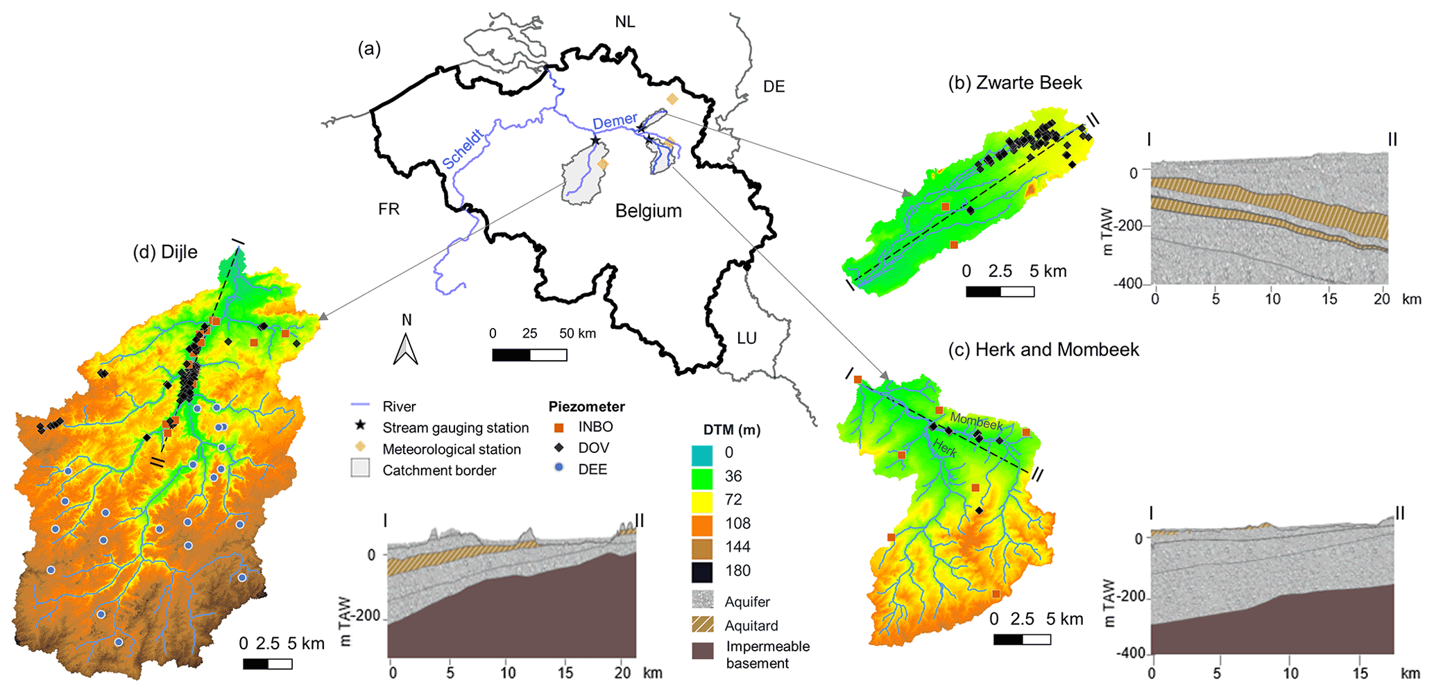
Figure 1Location of the studied catchments in (a) the Scheldt River basin, including (b) the Zwarte Beek, (c) the Herk and Mombeek, and (d) the Dijle, and the cross-sectional sketches of the hydrogeological layers (DOV, 2020) and piezometers in each catchment. The digital terrain model (DTM) is from Geopunt Vlaanderen (https://www.geopunt.be/, last access: 18 October 2020).
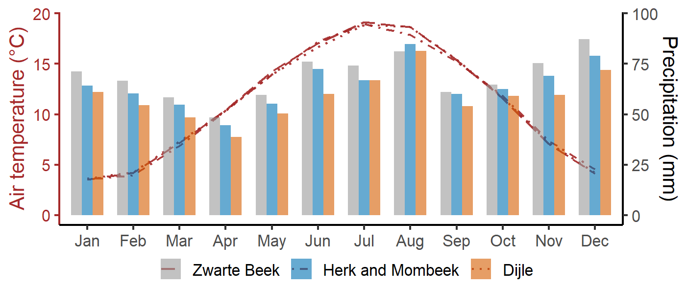
Figure 2The average monthly precipitation and air temperature of the three catchments, based on daily observations between 1990 and 2019 (KMI, 2020).
Both the Zwarte Beek and the Herk and Mombeek are tributaries of the Demer River (Fig. 1a). The Demer joins the Dijle at Rotselaar and then heads towards the Scheldt Estuary in Antwerp (Fig. 1a). The streamflows of the studied river segments are measured at the catchment outlet (Fig. 1a). The average daily streamflows are 1.05 m3 s−1 for the Zwarte Beek, 1.44 m3 s−1 for the Herk and Mombeek, and 6.65 m3 s−1 for the Dijle. The streamflow varies between 0.001 and 7.03 m3 s−1 for the Zwarte Beek, between 0.06 and 20.4 m3 s−1 for the Herk and Mombeek, and between 1.23 and 29.1 m3 s−1 for the Dijle (Fig. 3a). The flow duration curve (FDC) plots the cumulative frequency of the streamflow and represents the variability of streamflow in a catchment (Vogel and Fennessey, 1994), with a flat slope indicating a groundwater-feeding surface storage and a steep slope revealing a flashy flow regime dominated by direct runoff (Searcy, 1959). The flat slope of the FDCs (Fig. 3a) indicates that these perennial rivers have a strong groundwater-feeding feature. The monthly average streamflows show that there is some seasonality in the time series – specifically, higher flows are observed during the winter months (December–February) than during other seasons in all three catchments (Fig. 3b). For the Dijle catchment alone, the monthly average streamflows are relatively low in the spring (March–May) and relatively high in both the summer and winter during the 30-year study period (Fig. 3b).
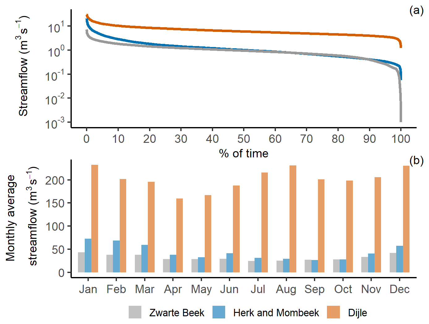
Figure 3The (a) flow duration curve (FDC) and (b) average monthly streamflow in the three catchments.

Figure 4An illustration of the methodology used in this study. PCA is the abbreviation for principle component analysis.
According to the Flanders subsurface database DOV (Databank Ondergrond Vlaanderen) and lithostratigraphic units, the Zwarte Beek catchment mainly developed in sandy Neogene sediments, and the Boom and Kortrijk Clay formations (Fig. 1b) represent two aquitards (DOV, 2020; Laga et al., 2001). The surficial geology outside the floodplain is dominated by sand, whereas the floodplain itself is dominated by sand and peat (DOV, 2020). The streambed material varies from coarse sand upstream to fine sand downstream, as observed during field trips. The Herk and Mombeek catchment (Fig. 1c) developed mostly in sandy Paleogene sediment with the Boom Clay Formation at shallow depth in the northern part (Laga et al., 2001). The top of the impermeable basement consists of marl and clay from the Heers and Hannut formations (DOV, 2020; Laga et al., 2001). The surficial geology outside the floodplain is dominated by loam and sandy loam, whereas the floodplain itself is characterized by loam and clay sediments (DOV, 2020). The riverbed of the Mombeek tributary consists mainly of clay, as observed during field trips. The Dijle Valley (Fig. 1d) mainly developed in Paleogene and Neogene sands, but continued incision is the reason why the floodplain has reached the very impermeable clay of the Kortrijk Formation below (DOV, 2020). The shallow geology outside the floodplain is dominated by loam and sandy loam deposits, and the floodplain itself consists of loam, sand, clay, and peat (DOV, 2020).
The major land uses are crop (24.4 %), meadow (23.6 %), and urban area (15.2 %) for the Zwarte Beek catchment; meadow (56.0 %), orchard (21.1 %), and crop (11.3 %) for the Herk and Mombeek; and crop (35.6 %), meadow (28.1 %), and urban area (19.7 %) for the Dijle in 2012 (DOV, 2020). The urban coverage is relatively low in all three catchments. The upstream area of the Zwarte Beek is within a military domain with little built-up area. There are also several natural reserves within these catchments. Since 1990, the Belgium government has carried out nature-based solutions for floodplain restoration and “zero management” polices to reduce the human impact on catchments such as the Dijle (Turkelboom et al., 2021); therefore, the three catchments mostly experienced natural conditions during the study period.
An illustration of the methodology is shown in Fig. 4. First of all, precipitation, air temperature, groundwater level, and streamflow data were collected and imputed where necessary. Afterwards, imputed precipitation and air temperature were used as system input for the first case in the impulse response model, and the system output was calibrated with the observed groundwater level. Only well-fitted groundwater level time series were retained and further used to generate a representative groundwater level time series via principle component analysis in each catchment. This time series was applied as system input for the second case in the impulse response model. The model output of simulated groundwater inflow to rivers was calibrated with separated baseflow obtained from hydrograph separation approaches. Finally, time series analysis was carried out to investigate the temporal variation, trend, and seasonality of the hydrological variables. Detailed explanations can be found in the following sections.
3.1 Data preparation
3.1.1 Data collection
The daily precipitation and daily air temperature were obtained from KMI (Koninklijk Meteorologisch Instituut) at the closest meteorological station for each catchment (Fig. 1a). The daily streamflow time series were accessed from https://www.waterinfo.be (last access: 10 March 2020) via the “wateRinfo” R package interface (Van Hoey, 2020) and from the river gauging station at the catchment outlet (Fig. 1a). These time series cover one climatic cycle of 30 years (1 January 1990–31 December 2019).
The groundwater levels were obtained from the piezometric observation network of INBO (Instituut voor Natuur- en Bosonderzoek), DOV, and DEE (Département de l'Environnement et de l'Eau) and represented 82 %, 11 %, and 7 % of the total number of 343 wells, respectively (Fig. 1b, c, d). The groundwater level time series from INBO are recorded daily. Mostly of the groundwater levels from the DOV are measured monthly, and the rest are recorded biweekly. The observations from the DEE are generally measured on a weekly basis, and the rest are measured on a monthly basis.
In the Zwarte Beek and the Herk and Mombeek, the average groundwater depths to the water table are 0.6 and 3.1 m, respectively, and the observations are all from shallow aquifers, with a groundwater depth to the water table of less than 17.8 m. In the northern Flemish part of the Dijle catchment, the groundwater level time series are located in the very shallow part of the aquifer, with an average depth to the water table of 1.1 m. In the southern Walloon region of the Dijle catchment, where the elevation differences are larger than in the north, we obtained a very limited number of observations (23) from DEE (Fig. 1d) and included them all to avoid data absence in that region. The groundwater depth to the water table there has a mean value of 25.3 m. The time spans of the groundwater level observations vary between 2 and 30 years, with an average of 16.2 years. Time series that covered short periods (e.g., a few months) or were very discontinuous were excluded. With a monthly frequency, time series consisting of at least 90 data points were considered to be adequate, which corresponded to one-fourth (7.5 years) of the full time period.
3.1.2 Data imputation
The missing values in the raw time series were imputed, as required for further analysis. The imputation techniques applied in this study were (1) linear or local polynomial regression models for estimations based on different time series and (2) ordered quantile normalization for rescaling different time series (Fan and Gijbels, 2018; Peterson and Cavanaugh, 2019). A time series of a nearby station that survived the quality checks and has less missing values is used as the reference series to check first if a linear regression model would be adequate (R2≥0.7). If it is not satisfactory, a local polynomial regression model is applied instead. When the linear regression model is not adequate, another option is to perform ordered quantile normalization. The marginal distribution of the target series is, in this case, approximated, using days with observations in both series, by transforming both with ordered quantile normalization and making the two distributions identical with respect to statistical properties (Peterson, 2021).
3.2 Baseflow separation
Baseflow separation divides the streamflow into the components that originate from (1) quick flow (the sum of water derived from precipitation that contributes to the stream soon after rainfall events) and (2) baseflow (groundwater discharge or other delayed sources) (Hall, 1968; Nathan and McMahon, 1990; Piggott et al. 2005). The main separation techniques include (1) graphic methods, which pick out the low-flow points from the hydrographs and link them together as the baseflow component (Sloto and Crouse, 1996; Rutledge, 1998), and (2) digital filter methods, which filter out a low-frequency signal representing baseflow and a high-frequency signal attributed to quick flow (Nathan and McMahon, 1990; Arnold and Allen, 1999; Eckhardt, 2005, 2008; Jakeman and Hornberger, 1993). The baseflow index (BFI) gives the ratio of the baseflow to the total streamflow. It is an indicator of the catchment flow regime, with high indices (>0.9) for permeable catchments with a very stable flow regime and low indices (0.15–0.2) for impermeable catchments with a flashy flow regime (Tallaksen and Van Lanen, 2004). Although it is difficult to validate the separated baseflow and there is lack of presentation of the physical processes of the river–aquifer exchange (Sloto and Crouse, 1996; Batelaan and De Smedt, 2007; Killian et al., 2019), baseflow separation is still a fast, efficient, and widely used approach to quantitatively estimate the baseflow at the catchment scale.
In this study, we used different baseflow separation methods to provide an idea of the range of potential outcomes. The selected approaches were (1) graphical separation techniques from HYSEP (Hydrograph Separation Program; Sloto and Crouse, 1996), including the fixed-interval, sliding-interval, and local-minimum technique; (2) the one-parameter digital filter method from Nathan and McMahon (1990), where the filter parameter is taken as 0.925; and (3) the two-parameter digital filter method from Eckhardt (2005, 2008), as this method agrees well with tracer-based (e.g., dissolved silica) hydrograph separation in lowland catchments (Gonzales et al., 2009). The filter parameter is set as 0.98, and the BFImax parameter is chosen as 0.80 for the Eckhardt method, as recommended by other research conducted using the same method in Flanders (Zomlot et al., 2015).
3.3 Impulse response modeling
3.3.1 Model overview
A lumped parameter impulse response model can effectively transform a hydrological system input to yield an accurate prediction of the corresponding system output, and the impulse response function (IRF) estimated in the model can provide mechanistic insights into the hydrological system, such as the peak response time and magnitude (Olsthoorn, 2007; von Asmuth and Knotters, 2004; Young, 2013). The impulse response model used in this study is the Rainfall-Response Aquifer and Watershed Flow Model (RRAWFLOW; Long, 2015). RRAWFLOW includes two processes: (1) the process of recharge generation from precipitation, denoted as precipitation recharge in this study, and (2) the process of precipitation recharge transitioning into a system response such as groundwater level or spring flow (Long and Mahler, 2013; Long, 2015).
During the first nonlinear process, the precipitation recharge is estimated using a unitless soil–moisture index, s (Long and Mahler, 2013). This s (≤1.0) represents the fraction of precipitation that infiltrates and becomes precipitation recharge. As the preceding rainfall events have impacts on soil moisture, the past rainfall record is counted and weighted by an exponential decay function (Jakeman and Hornberger, 1993). Detailed equations and parameterization can be found in Long and Mahler (2013).
During the second process, the response of the hydrological system to the precipitation recharge is estimated by convolution (Long, 2015), which is the superposition of a series of IRFs that are initiated at the time of each impulse and scaled proportionally by the magnitude of the corresponding impulse (Olsthoorn, 2007; Long and Mahler, 2013; von Asmuth et al., 2002). The discrete form of the convolution integral for uniform time steps used in RRAWFLOW is
where hi−j is the IRF; uj is the input; j and i are time step indices corresponding to system input and output, respectively; Δt (T) is the time step duration; N (unitless) is the number of time steps in the output record; βj (unitless) is an optional scaling coefficient of IRF; ψi is the error component resulting from inaccuracy in measurement, sampling intervals, or model simplification assumptions; and d0 is a hydraulic-head datum (L) for groundwater level simulation (Long, 2015). In this process, precipitation recharge (uj) is assumed to be the only forcing that can cause an increase in the hydraulic head to be above d0 (Long, 2015).
Hydrological system dynamics can be approached by different types of parametric IRFs. In this study, we use parametric gamma functions, as they tend to work well and allow us to easily evaluate the fitted parameters. The gamma function and gamma distribution function in RRAWFLOW are as follows:
Here, Γ and γ are the gamma function and gamma distribution function, respectively; λ (unitless) and η (unitless) are shape parameters; t (T) is the time centered on each discrete time step; h is the scaled gamma distribution function; and ϵ (unitless) is the scaling coefficient that compensates for the system response when there is not a one-to-one relation between system input and output (Olsthoorn, 2007; Long, 2015). RRAWFLOW allows the use of two superposed gamma distribution functions, which represent the components of quick flow and slow flow in the hydrological system, and it also allows the system records to be divided into two periods, namely dry and wet periods (Long, 2015).
The “L-BFGS-B” (limited-memory Broyden–Fletcher–Goldfarb–Shanno bound) method is used for RRAWFLOW optimization, which allows one to work with lower and upper parameter bounds (Byrd et al., 1995). The Nash–Sutcliffe efficiency (NSE) is used for the evaluation of the simulated time series (Nash and Sutcliffe, 1970). A NSE of 1 means a perfect model fit, a NSE of 0 indicates that the model has the same predictive power as the mean of the time series in terms of the sum of the squared error, and NSE < 0 means that the predictive power is worse than that of the observed mean (Nash and Sutcliffe, 1970).
We use RRAWFLOW to explore the hydrological system response of groundwater level to meteorological forcing (Sect. 3.3.2) and groundwater inflow response to groundwater level as system input (Sect. 3.3.3), under natural conditions. The model parametrization and modifications to the original RRAWFLOW code are discussed below.
3.3.2 Groundwater level response modeling
Groundwater level response modeling consists of precipitation recharge generation and recharge transitioning into groundwater level. The system input is precipitation and air temperature data, and the system output is compared with groundwater level observations. The model time step interval is daily, which is determined by the input time series of precipitation and air temperature. A warm-up period of 6 years was added (1984–1989), using the data record from the first 6 years (1990–1995). This estimated warm-up period can largely reduce the antecedent effects of the system before it is fully incorporated into the simulation.
To better represent the transient characteristics of the hydrological system, the dry (April–September) and wet (October–March) periods are defined, due to the very different evapotranspiration effects within the year (Fig. 2). Different gamma distribution functions are also used to represent quick and slow components. In total, four gamma distribution functions are used in the simulation, representing the quick flow and slow flow processes during both the dry and wet periods. In each gamma distribution function, there are three parameters to be optimized: two shape parameters (λ and η, Eq. 3) and one scaling coefficient (ϵ, Eq. 4). The double-gamma IRFs representing dry (hdry) and wet (hwet) periods are shown below:
Here, the subscripted numbers “1” and “2” are used for the respective quick and slow components during dry period, and “3” and “4” are used for the respective quick and slow components during the wet period. Besides the 12 parameters from the IRFs (Eqs. 5, 6), the hydraulic-head datum parameter (d0, Eq. 1) is also included for optimization.
Although the IRFs can have infinite length, we define that the system has a maximum memory of 6 years for an impulse in order to avoid long-term trends or human interference effects from biassing the fitted IRFs. The whole 30-year period is used for model calibration, as we are doing exploratory rather than confirmatory analysis here.
3.3.3 Groundwater inflow response modeling
Groundwater inflow response modeling simulates the process of groundwater discharge to rivers. Fitted groundwater levels from the previous step are used for this process. As there are many groundwater level time series in each catchment, we introduce a single representative groundwater level time series in order to reduce the dimensionality of the problem. The representative groundwater level time series was obtained by extracting the first principle component of the fitted groundwater level time series, so as to represent the catchment status in terms of groundwater level.
The model was set up with the representative groundwater level as the system impulse and separated baseflow as the system response. A 6-year warm-up period (1984–1989) was again added, using the representative groundwater level time series for the period between 1990 and 1995. As the groundwater discharge to streamflow happens beneath the land surface, without the pronounced wet–dry period distinctions from the effects of evapotranspiration, a time-invariant model is assumed for this modeling process. Thus, only two gamma distribution functions are used to represent the quick and slow components. The compound IRF (hcomp) is shown below:
where the subscripted letters “q” and “s” represent the quick and slow components, respectively.
Furthermore, a modification is made to the original code: a constant drainage level is subtracted from the input groundwater level. This operation turns the representative groundwater level into a proxy for the hydraulic gradient. The modified convolution integral has the following form:
Hence, there are seven parameters to be optimized: three parameters (λ, η and ϵ) for each of the two gamma distribution functions and the drainage level, which was actually implemented by using the hydraulic-head datum d0. This allowed the modification to be made with minimal code adjustments.
3.4 Time series analysis
Hydrological time series usually have strong seasonal variations and can be decomposed using an additive approach to study the temporal evolution of the different components. In this study, we apply the Seasonal and Trend decomposition with Loess (STL) method to decompose the time series into three components: (1) a trend-cycle component, (2) a seasonal component, and (3) a reminder component (Cleveland et al., 1990). The additive decomposition of the target time series has the following form:
where yt is the seasonal time series, Tt is the smoothed trend-cycle component, St is the seasonal component, and Rt is the remainder component (Cleveland et al., 1990).
The features of the STL decomposition are summarized using two parameters:
-
the strength of the trend, calculated as
with Ft close to 0 representing a weak trend and Ft close to 1 representing a strong trend; and
-
the strength of the seasonality, calculated as
with Fs close to 0 indicating weak seasonality and Fs close to 1 indicating a strong seasonality (Hyndman and Athanasopoulos, 2021).
The decomposed hydrological variables include precipitation, representative groundwater level, streamflow, and separated baseflow. The trend analysis uses a window of 365 consecutive daily observations to estimate the trend-cycle component on a yearly basis. This span allows for the retention of sufficient fluctuation in the data. The seasonal component analysis takes 365 d as its periodic cycle and a window of 11 consecutive years for estimating the seasonality.
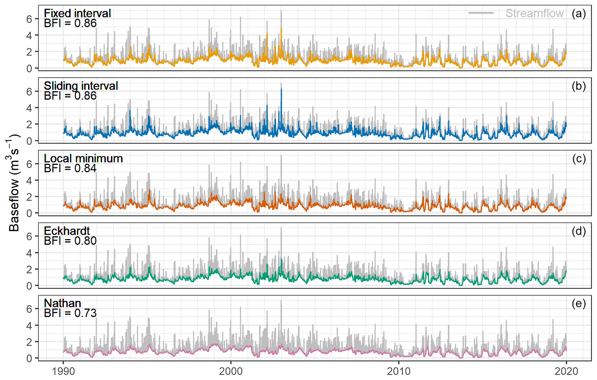
Figure 5The separated baseflow and streamflow time series over the 30-year study period in the Zwarte Beek.
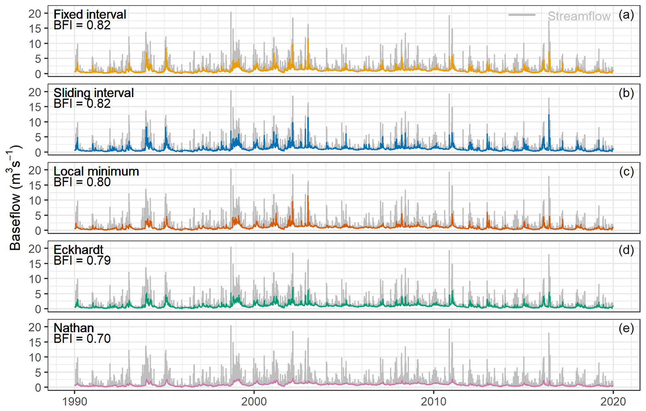
Figure 6The separated baseflow and streamflow time series over the 30-year study period in the Herk and Mombeek.
4.1 Separated baseflow
Figures 5–7 show the temporal evolution of the separated baseflow on a daily basis and the comparison of the streamflow and baseflow using different methods in the three catchments. The fixed-interval and sliding-interval approaches yield slightly higher estimated mean BFIs than other methods, as they capture quite a large amount of baseflow from the peak flows and high-flow periods in the streamflow record (panels a and b in Figs. 5–7). The local-minimum and Eckhardt methods result in slightly lower mean BFIs than the previous two methods, as they tend to filter out the large impact of high-streamflow events on the baseflow (panels c and d in Figs. 5–7). The estimated mean BFI from the Nathan approach is the lowest among all the methods, and the separated baseflow time series has less amplitude variation over time and is less influenced by high streamflows than the other methods (Figs. 5e, 6e, 7e). The mean BFIs over the 30-year period range between 0.73 and 0.86 for the Zwarte Beek, between 0.70 and 0.82 for the Herk and Mombeek, and between 0.77 and 0.84 for the Dijle.

Figure 7The separated baseflow and streamflow time series over the 30-year study period in the Dijle.
4.2 Impulse response modeling of the hydrological system
4.2.1 Groundwater level response modeling
Altogether, 100 groundwater level time series in the Zwarte Beek, 45 in the Herk and Mombeek, and 198 in the Dijle were used for the groundwater level response modeling. The positive NSEs (0–1) of the simulated time series comprise 89 %, 95 %, and 83 % of all the simulations in the Zwarte Beek, the Herk and Mombeek, and the Dijle, respectively. The overall model performance is better in the Zwarte Beek and the Herk and Mombeek than in the Dijle. Considering the balance between evaluating model performance and allowing sufficient simulated time series to compute the representative groundwater level, we considered the simulations with a NSE > 0.3 as satisfactory. This allowed 70 simulated time series for the Zwarte Beek, 38 for the Herk and Mombeek, and 108 for the Dijle to be retained. Examples of the retained groundwater level time series for each catchment are shown in Fig. 8. The time series for the Zwarte Beek and the Herk and Mombeek (Fig. 8a, b) seem to be reproduced by the impulse response model in a very detailed way (NSEs > 0.8), whereas the time series for the Dijle (Fig. 8c) seems to exhibit very low levels in the middle or second half of the year and can apparently not be captured in a straightforward manner with impulse response modeling.
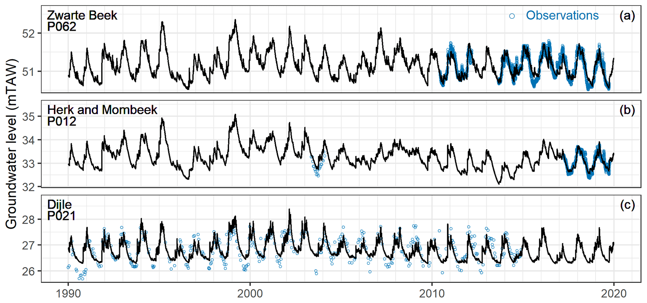
Figure 8Selected observed and simulated groundwater level time series for impulse response modeling: (a) ZWAP062 in the Zwarte Beek (NSE = 0.838), (b) MOMP012 in the Herk and Mombeek (NSE = 0.857), and (c) DYLP021 in the Dijle (NSE = 0.583).
The IRF curves from the modeling are shown in Fig. 9 for each retained groundwater level time series for the three catchments. Based on these IRFs, we extracted the peak time, representing the time it takes for the groundwater level response to reach its maximum value due to precipitation recharge, and the corresponding peak response (Fig. 10).
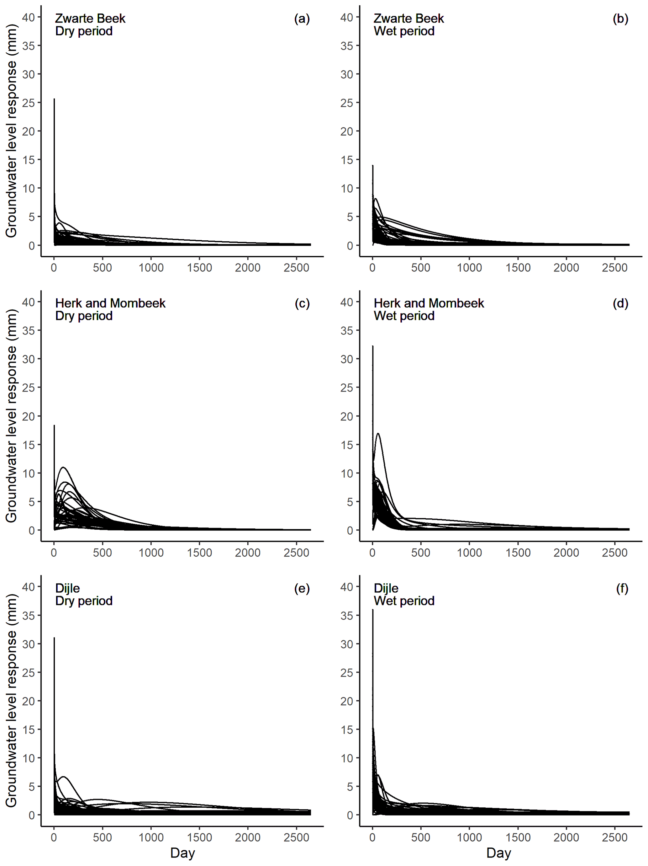
Figure 9Impulse response functions (IRFs) derived from the groundwater level response modeling for the dry (April–September) and wet (October–March) periods in the three catchments.
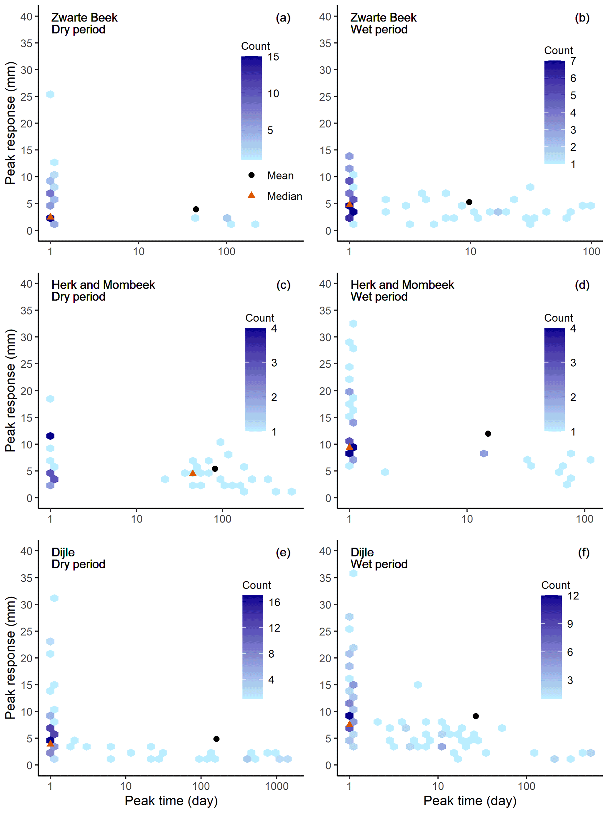
Figure 10Peak time and peak groundwater level response derived from the groundwater level response modeling for the dry (April–September) and wet (October–March) periods in the three catchments.
In the Zwarte Beek, approximately 73 % (51 of 70) of the retained groundwater level wells in the dry period (April–September) and 61 % (43 of 70) of the retained groundwater level wells in the wet period (October–March) reached their peak response on the first day (panels a and b in Figs. 9–10). This indicates a very fast response to precipitation recharge in the shallow aquifer. The rest of the level time series had a peak time ranging between 2 and 548 d during the dry period (Fig. 10a) and between 2 and 98 d during the wet period (Fig. 10b). On average, it takes 45 d in the dry period (Fig. 10a) and 10 d in the wet period (Fig. 10b) for the shallow aquifer to obtain its maximal response to precipitation recharge. For the response magnitude, 1 mm of precipitation recharge can cause a maximal immediate groundwater level rise of between 0.01 and 25.7 mm during the dry period (Fig. 10a) and of between 0.8 and 14.0 mm during the wet period (Fig. 10b). The mean peak responses are 3.9 and 5.3 mm for the dry and wet seasons, respectively (Fig. 10a, b). A relatively higher immediate increase in the groundwater level occurs in the wet period compared with the dry period.
In the Herk and Mombeek, around 42 % (16 of 38) of the groundwater level time series in the dry period and 71 % (27 of 38) of the groundwater level time series in the wet period reached their peak response on the first day (panels c and d in Figs. 9–10). For the rest, the range of the peak time is larger in the dry period (2–570 d; Fig. 10c) than in the wet period (2–104 d; Fig. 10d). The mean peak time is 81 and 15 d for the dry and wet periods, respectively (Fig. 10c, d). Therefore, there is a clear trend toward a much faster response of the shallow aquifer to precipitation recharge in the wet period than in the dry period. Regarding the peak response magnitude, the range is between 0.8 and 18.4 mm for 1 mm of precipitation recharge in the dry period (Fig. 10c) and between 2.6 and 32.3 mm in the wet period (Fig. 10d). The mean peak magnitudes are 5.4 and 12.0 mm for the dry and wet periods, respectively (Fig. 10c, d). There is a general spatial trend observed in this catchment. If an observation well is closer to the river or the groundwater depth to the water table is smaller, the peak time is relatively shorter and the peak response is higher.
During the dry period in the Dijle, approximately 68 % (73 of 108) of the observation wells reached their peak response on the first day, whereas the remaining wells varied between 2 and 574 d (Figs. 9e, 10e). During the wet period, around 59 % (64 of 108) of the observation wells reached their peak response on the first day, and the other wells peaked between 2 and 528 d (Figs. 9f, 10f). The mean peak time is 159 and 27 d for the dry and wet periods, respectively (Fig. 10e, f). The peak response ranges between 0.02 and 31.1 mm for the dry period (Fig. 10e) and between 0.6 and 36.1 mm for the wet period (Fig. 10f) for 1 mm of precipitation recharge. The mean peak response magnitudes are 4.9 and 9.2 mm for the dry and wet periods, respectively (Fig. 10e, f).
4.2.2 Groundwater inflow response modeling
The retained groundwater level time series from the previous simulations are used to generate a time series of the groundwater level in order to represent groundwater storage over the entire catchment. The extracted first principle component of the simulated groundwater levels explains 83 %, 91 %, and 79 % of the total variance for the Zwarte Beek, the Herk and Mombeek, and the Dijle, respectively (Fig. 11b, d, f). The representative groundwater level time series has a mean of zero, and the level is rescaled to a relative elevation (in meters, dividing the scores of the first principle component by the sum of the loadings) because only the level differences are relevant for the groundwater inflow response modeling (Fig. 11a, c, e). This time series can be interpreted intuitively as the relative difference between the groundwater level across the catchment at a certain point in time and the average groundwater level.
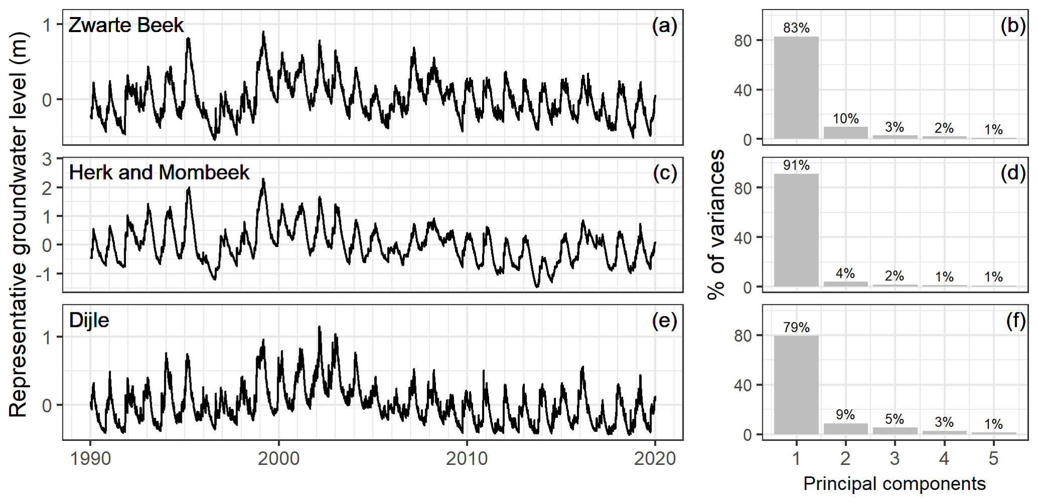
Figure 11The representative groundwater level (relative elevation) time series and the variance proportions of the first five principle components in each catchment.
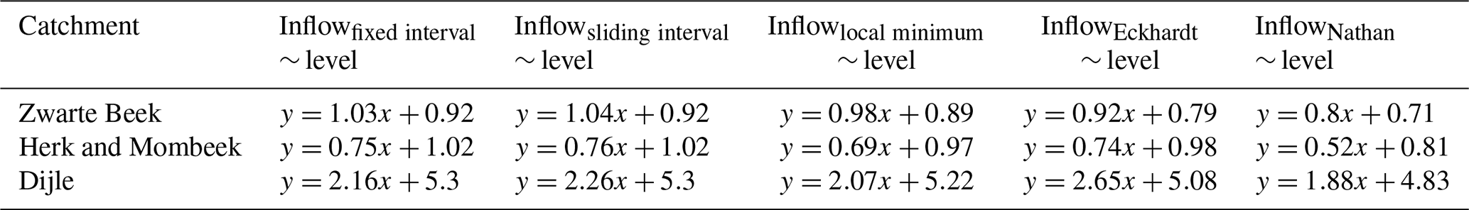
The mean NSEs of simulated baseflow time series are 0.325 for the Zwarte Beek, 0.384 for the Herk and Mombeek, and 0.146 for the Dijle. The Eckhardt and Nathan methods work better than other methods in the Zwarte Beek, with NSE values of 0.385 and 0.377, respectively. The Nathan method yields a higher NSE of 0.478 than other methods in the Herk and Mombeek. In the Dijle, the Eckhardt method performs better than other methods, with a NSE of 0.212. The IRFs extracted from the modeling show that there is basically an immediate response in the first time step, and the responses for a few days are already negligible. This means that our impulse response model basically falls back to a linear regression model of the groundwater inflow as a function of the representative groundwater level, where the intercept and the slope are related to the drainage level and impulse response function value for the first time step, as shown in Table 1. The mean peak response, calculated as the mean value of the slopes in Table 1, shows an average change of 0.95 m3 s−1 of baseflow in the Zwarte Beek, 0.69 m3 s−1 in the Herk and Mombeek, and 2.2 m3 s−1 in the Dijle as a response to a 1 m change in the groundwater level.
Table 1The linear regression fit of the groundwater inflow as a function of the representative groundwater level in each catchment. The term “level” refers to the representative groundwater level; “Fixed interval”, “Sliding interval”, “Local minimum”, “Eckhardt”, and “Nathan” refer to the different separation techniques.
The simulated time series of groundwater inflow to the river tend to be smoother than the separated baseflow time series (Figs. 12, 13, 14). For the Zwarte Beek, the simulated groundwater inflow for the first 2 decades (1990–2009) can capture most of the low points, whereas there are some continuous periods with overestimation for the last decade (2010–2019) (Fig. 12). In the Herk and Mombeek, the simulated groundwater inflow time series seem to match well with the separated baseflow between 2005 and 2010, and major model overestimation occurs in the first decade (Fig. 13). For the Dijle, the differences between the simulated groundwater inflow and separated baseflow are relatively large compared with the other catchments. For periods with decreased or increased fluctuations in separated baseflow (e.g., 1996–1999 or 2000–2008), the groundwater inflow variation is less intense (Fig. 14).

Figure 12The comparison between the simulated groundwater inflow and the separated baseflow in the Zwarte Beek.
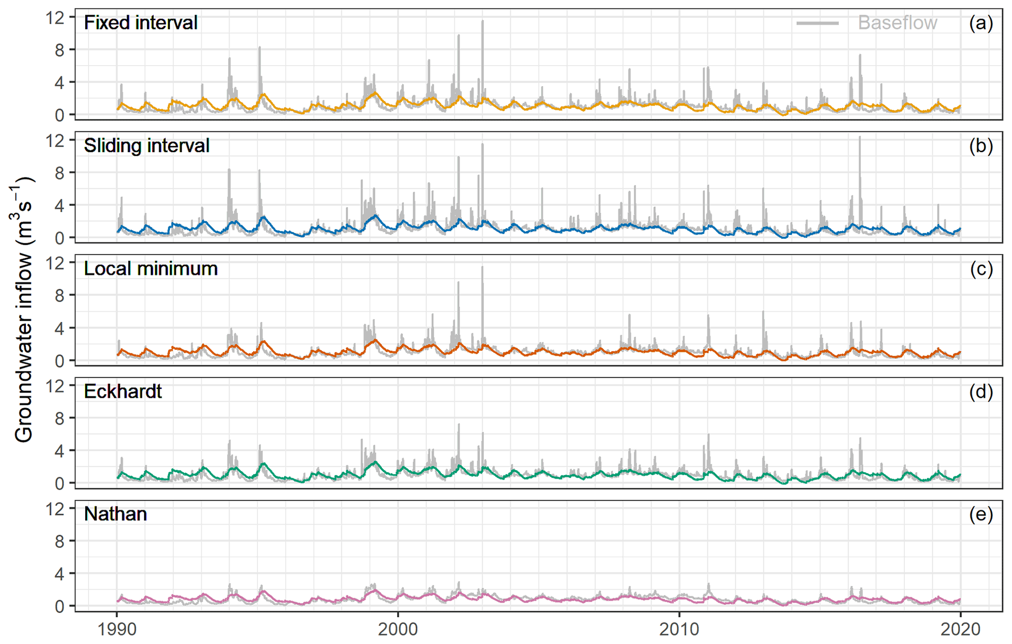
Figure 13The comparison between the simulated groundwater inflow and the separated baseflow in the Herk and Mombeek.

Figure 14The comparison between the simulated groundwater inflow and the separated baseflow in the Dijle.
4.3 Time series analysis
Precipitation has little trend over the 30-year period, and the magnitudes of the extracted trend components are much smaller than the raw time series (Figs. 15a, 16a, 17a, 18). There is some level of seasonality observed for precipitation, and the amplitudes of the seasonal components vary a lot between different years (Figs. 15b, 16b, 17b, 18). The representative (Rep.) groundwater level time series has a strong trend and seasonal strengths, and it is located in the cluster formed by the individual (Indiv.) groundwater level time series, which indicates that it is a good representation of the catchment status in terms of groundwater level (Fig. 18). The trend component curve itself does not show a continuous positive nor negative trend over the whole 30-year period; rather, it demonstrates varying trend directions during different periods (Figs. 15c, 16c, 17c). The seasonal strength of the representative groundwater level is close to that of the air temperature (Fig. 18). The streamflow demonstrates some level of trend and seasonality (panels e and f in Figs. 15–17). The trend and seasonal strengths of the separated baseflow time series are moderate, and the different baseflow time series fall somewhere between the streamflow and representative groundwater level (Fig. 18). This indicates that there is a range of outcomes, in terms of trend and seasonal components, that varies from more similar to the streamflow characteristics to closer to the representative groundwater level characteristics. It seems that the Nathan approach provides baseflow with a closer link to the representative groundwater level.
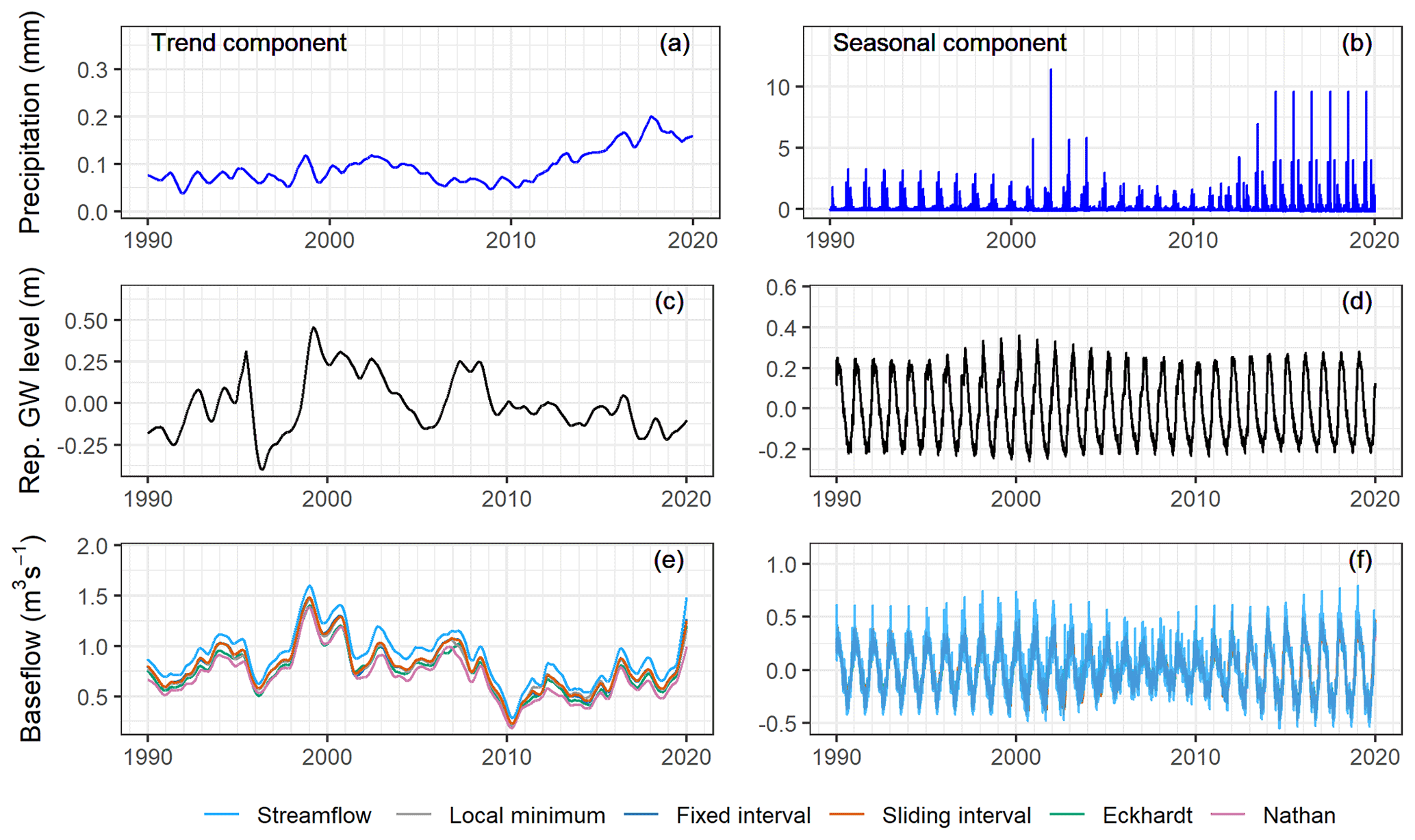
Figure 15The trend and seasonal components of the decomposed precipitation, representative groundwater level, streamflow, and separated baseflow in the Zwarte Beek.
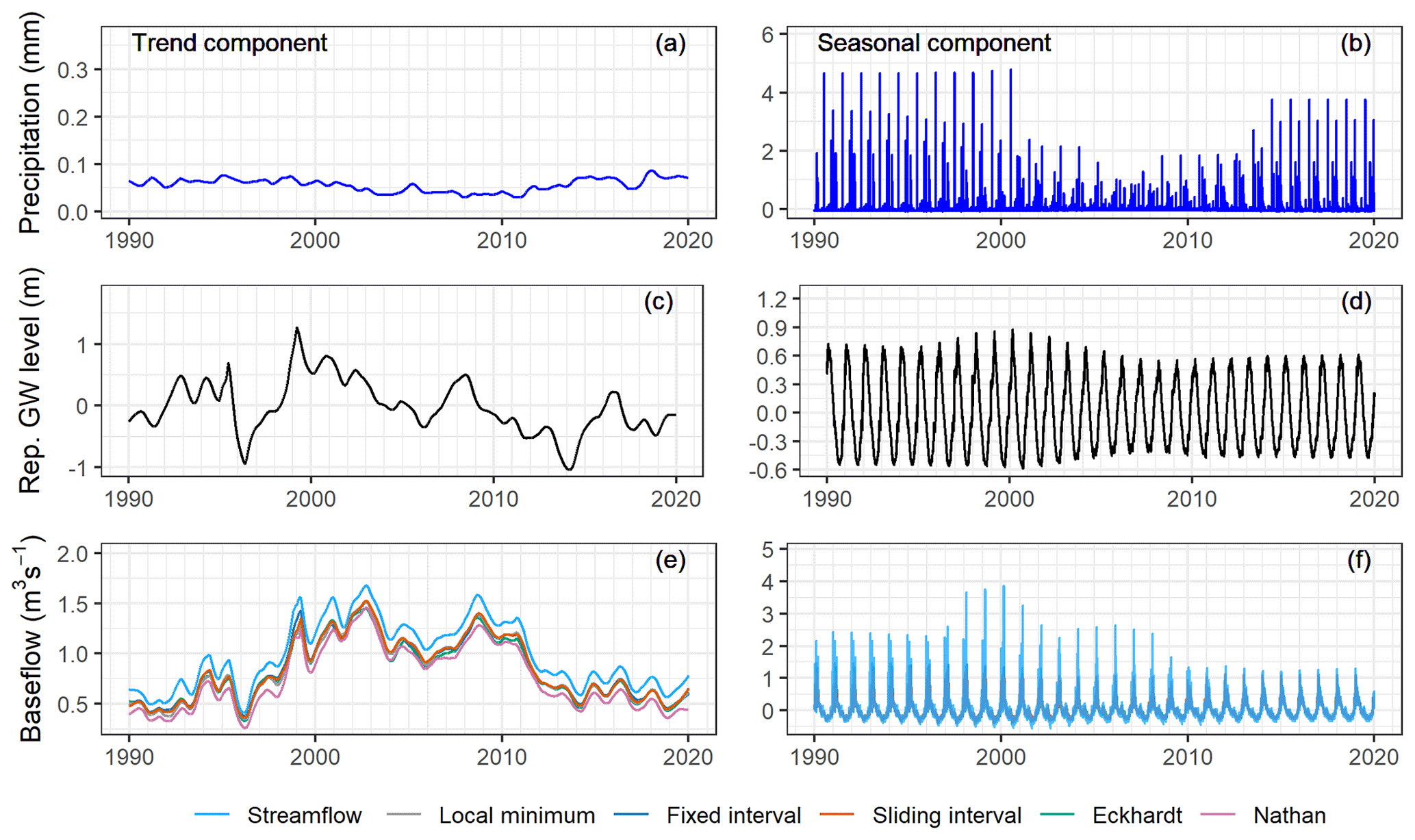
Figure 16The trend and seasonal components of the decomposed precipitation, representative groundwater level, streamflow, and separated baseflow in the Herk and Mombeek.
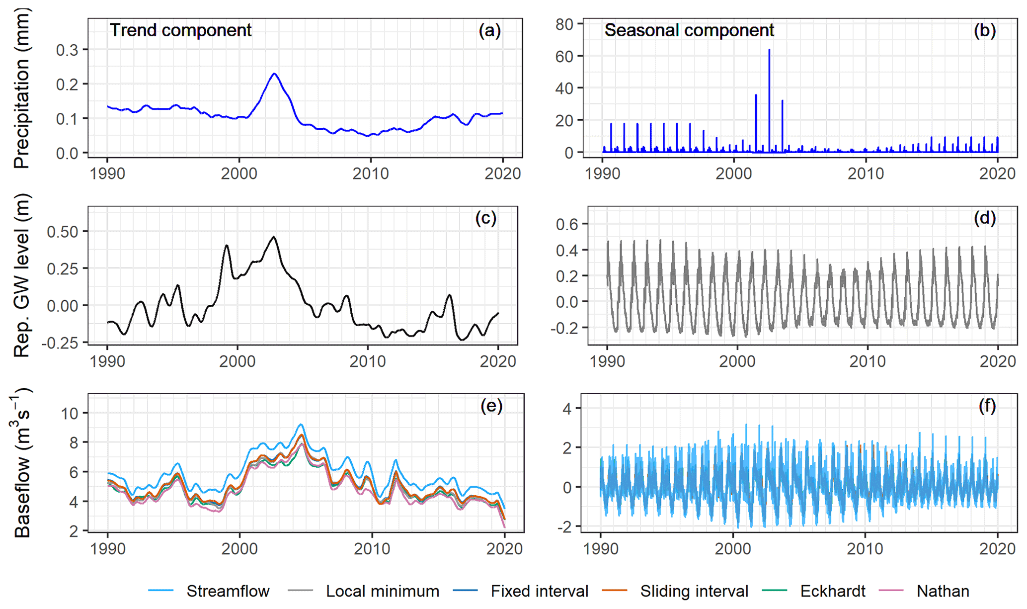
Figure 17The trend and seasonal components of the decomposed precipitation, representative groundwater level, streamflow, and separated baseflow in the Dijle.
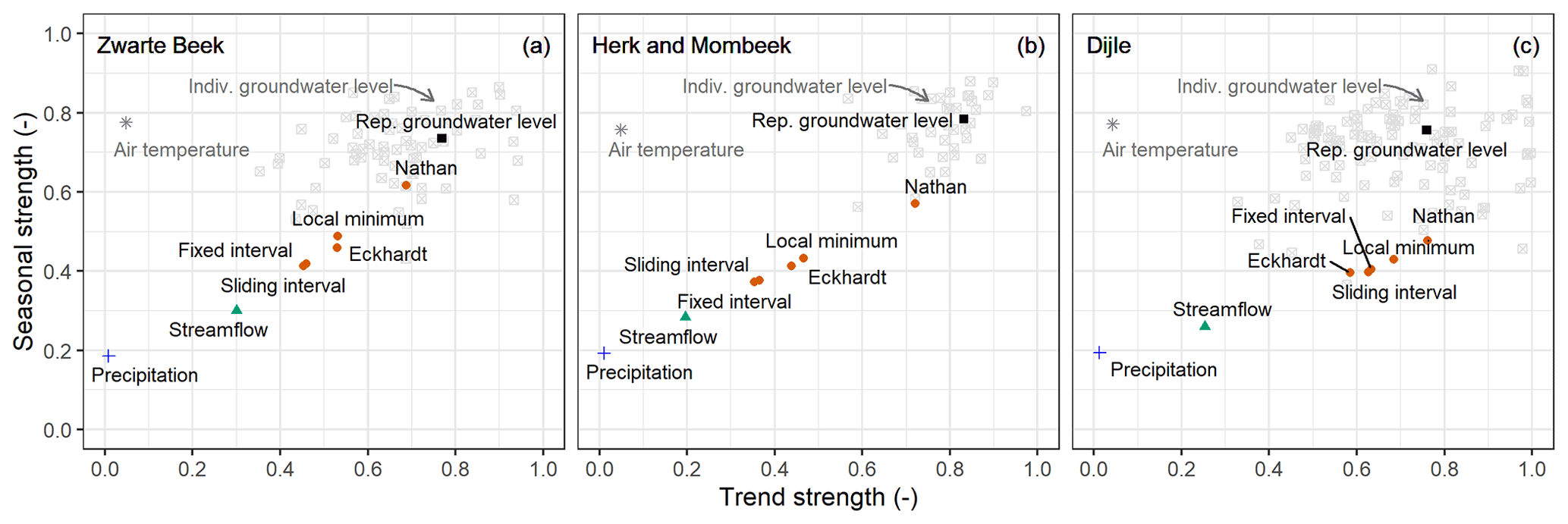
Figure 18Trend and seasonal strengths of the precipitation, air temperature, representative groundwater level, individual groundwater level, streamflow, and separated baseflow in the three catchments.
5.1 Baseflow and groundwater inflow estimation
As important indicators of river–aquifer interactions, baseflow and groundwater inflow to rivers are estimated here using the streamflow record and the groundwater level, respectively. However, the estimation of groundwater inflow to rivers still relies on the baseflow estimation, as separated baseflow is used as the dependent variable in the modeling exercise.
Baseflow separation is a subjective process that is based on different mathematical techniques, rather than the physical processes governing river–aquifer exchange (Sloto and Crouse, 1996; Batelaan and De Smedt, 2007; Killian et al., 2019). Three methods from HYSEP select the minimum values of the hydrograph with an interval using different algorithms (Sloto and Crouse, 1996). Alternatively, the Nathan and Eckhardt methods use parameters that have some physical connection to the catchment characteristics, such as the flow status of streams within the year (perennial or ephemeral) and the permeability of the aquifers (Nathan and McMahon, 1990; Arnold and Allen, 1999; Eckhardt, 2005).
Despite the methodological differences, the mean BFIs of the separated baseflow time series are never less than 0.70 in the three catchments (Figs. 5, 6, 7). These high BFIs indicate that the studied catchments are groundwater-dominated lowland systems, which is also reflected in the flat slope of the FDCs (Fig. 3a). The mean BFI ranges of the three catchments agree well with a previous study by Batelaan and De Smedt (2007), where the range are 0.81–0.83 for the Zwarte Beek, 0.79–0.81 for the Demer (the Herk and Mombeek is part of Demer), and 0.81–0.87 for the Dijle, using the Sloto and Crouse method (Sloto and Crouse, 1996). In our study, the Eckhardt and Nathan methods generate relatively smooth baseflow time series when compared to the graphical HYSEP methods (Figs. 5, 6, 7). Zomlot et al. (2015) conducted baseflow separation in 11 selected regional catchments in Flanders and also found that the one- or two-parameter recursive digital filter methods generated slightly lower mean BFIs than the local-minimum method from HYSEP.
Estimated groundwater inflow time series through impulse response modeling can capture part of the variation in the separated baseflow but do not reproduce the peaks in the separated baseflow very well. This is consistent with the fact that the separated baseflow from hydrographs is actually the total baseflow, which includes groundwater inflow as well as other slower-moving water that sustains streamflow between rainfall events. The difference between the separated baseflow and the obtained groundwater inflow can roughly be seen as the delayed water release from storages other than those in the aquifer. In this context, the impulse response modeling approach from the groundwater flow perspective can allow one to estimate the groundwater inflow to the river and separate it from the total baseflow.
5.2 Impulse response modeling of the hydrological system
To the best of our knowledge, this is the first study that has used a two-step approach with lumped parameter impulse response modeling to estimate groundwater inflow to rivers in a temperate lowland hydrological system.
For the groundwater level response modeling process, the lowland aquifers react rather fast to the system input. A large number of wells reach their peak response during the first day in the three catchments. For the sake of comparison, we give the response time in groundwater level due to precipitation recharge, estimated in another study (Gonzales et al., 2009) using the impulse response functions by Venetis (Venetis, 1970) and Olsthoorn (Olsthoorn, 2007). A confined coarse sandy aquifer in a Dutch lowland catchment, with an average length of 800 m, average thickness of 10 m, hydraulic conductivity of 30 m d−1, and storativity of , has a groundwater response delay of approximately 16 h (0.67 d) for a precipitation event of around 8 mm (Gonzales et al., 2009). This is consistent with the fast-response behavior of most wells in our simulations, with a peak response during the first day. As the time step of our model is daily, we are not able to capture a peak response time shorter than 1 d. If the model input and level observation time series have a higher resolution, the peak response time will probably be less than 1 d, especially for the shallow unconfined lowland aquifers.
In the Herk and Mombeek, we observed the tendency for a faster and higher peak response when the well was closer to the river and the groundwater depth was closer to the surface. As the majority of the groundwater level wells were closer to the striped alluvial clay sediment along the river, we saw an impact of the sediment materials on the impulse response. When rainfall events occur, a shallow well close to the river experiences some buffering effect from the clayey sediment in the floodplain close to the river, which delays the process causing the activated groundwater to flow quickly towards the river. This can lead to a faster and higher response in the near-river groundwater level.
During the groundwater inflow response modeling, the system response is fast and linear. As mentioned before, estimating groundwater inflow from a groundwater perspective can be a promising option. However, further research is recommended to improve the simulation. When extracting the first principle components from the simulated groundwater level time series, more weight can be assigned to wells located close to the river and less weight can be given to wells at a distance, for instance, as shallow groundwater closer to the river tends to follow local pathways and contributes more to the river. This makes the generated groundwater level more representative of the near-river status. A second improvement can be made in the model itself: instead of using a constant drainage level, dynamic drainage level time series could, for instance, be included by adjusting relevant input codes.
5.3 Time series analysis
Although there have been several observed drought events in Europe in recent years (e.g., 1992, 2003, 2015, and 2018) (Hänsel et al., 2019; Fu et al., 2020), and our annual precipitation time series show low levels for some years in Belgium (e.g., 1996, 2003, 2013 and 2018), the precipitation trend is still small over the 30-year observation window. Under temperate humid climates, precipitation has some seasonal variations, but these variations are not strong. On the contrary, the trend and seasonality in the groundwater level time series are pronounced. This is due to the strong seasonal impacts of air temperature, which heavily influences the evapotranspiration process in the unsaturated zone. When the precipitation recharge reaches the shallow aquifer, the groundwater level time series inherits similar seasonal patterns from air temperature. Thus, we observe strong seasonality in the representative groundwater level time series.
The trend and seasonal strengths in streamflow lay between the two ends of precipitation and groundwater level (Fig. 18), which agrees with the fact that streamflow is the end product of the combined influences of groundwater inflow, precipitation, and other flow components. We also observe that groundwater inflow to rivers is a process in which the groundwater (in terms of the representative groundwater level), with strong trend and seasonal strengths, contributes to the streamflow, where the trend and seasonal signals are intervened by the quick flow component, leading to a weak trend and seasonality in streamflow (Fig. 18). From the groundwater inflow response modeling perspective, the groundwater inflow to rivers is a fast process, and it tends to carry a relatively strong trend and seasonal strengths from the groundwater as well as contributing to the total baseflow. The differences in the trend and seasonality strengths of the baseflow and groundwater level are the influences of other delayed sources contributing to baseflow. As the trend and seasonality of the baseflow from the Nathan method are closer to those of the groundwater level, it is more in line with the groundwater inflow from the groundwater-level-based approach, and it may be the best baseflow separation method to estimate groundwater inflow in this context.
Through a combined approach of baseflow separation, impulse response modeling, and time series analysis, we gained better insights into the river–aquifer interactions and the lowland hydrological system in the three catchments.
The graphical HYSEP (fixed-interval, sliding-interval, and local-minimum methods) and recursive digital filter approaches (Nathan and Eckhardt methods) yield high mean BFIs (≥0.70), indicating a strong groundwater-dominated feature in the study area. The recursive digital filter methods generate a relatively smoother baseflow time series than the graphical HYSEP ones.
We explored the lowland hydrological system with impulse response modeling using two steps: (1) the groundwater level response to system input of precipitation and air temperature and (2) the groundwater inflow response to system input of groundwater level. For the first process, the groundwater level in shallow aquifers reacts fast to the system input, with most of the wells reaching their peak response during the first day. There is an overall trend toward a faster response time and higher response magnitude in the wet than in the dry periods in the study areas. In the Herk and Mombeek, the streambed and stream bank consist of clay materials, which have some buffering effects for the near-river hydraulic interactions. Thus, there is a tendency toward a faster peak time and higher peak response when the well is closer to the river and the groundwater depth is closer to the surface.
During the second process, the system response is fast, and the simulated groundwater inflow can capture some variations, although not the peaks of the separated baseflow. The differences between the separated baseflow and the simulated groundwater inflow is delayed water release from other intermediate storages. As the groundwater inflow estimation from the groundwater perspective considers the physical connection between the river and aquifer in the subsurface to some extent, it can be an alternative method to assess the groundwater contribution to rivers.
The trend and seasonality analysis of the time series shows that the groundwater inflow to rivers is a process in which the strong trend and seasonal characteristics of the groundwater level are intervened by the quick flow component, resulting in streamflow with a weak trend and seasonality. By comparing the strengths of the decomposed components, the Nathan approach seems to provide baseflow estimates that are more closely related to groundwater inflow in this lowland setting.
Based the performance of the combined approach at our study sites, we consider that this approach has further potential to be applied to similar lowland catchments with small area coverages under natural conditions or under conditions with limited human impacts.
The RRAWFLOW code is publicly available at https://www.usgs.gov/centers/dakota-water/science/rrawflow-rainfall-response-aquifer-and-watershed-flow-model?qt-science_center_objects=7#qt-science_center_objects (US Geological Survey, 2020; Long, 2015). R functions from the “DVstats” (https://github.com/USGS-R/DVstats; Lorenz, 2017), “EcoHydRology” (https://github.com/cran/EcoHydRology; Fuka et al., 2018), and “FlowScreen” (https://CRAN.R-project.org/package=FlowScreen; Dierauer and Whitfield, 2019) packages are available for baseflow separation using the HYSEP, Nathan, and Eckhardt methods, respectively.
Meteorological input data (precipitation and air temperature) can be obtained upon request from KMI (Koninklijk Meteorologisch Instituut). Streamflow data are available at https://www.waterinfo.be (Flanders Environment Agency (VMM) and Flanders Hydraulics Research, 2020) and can be downloaded via the “wateRinfo” R package interface (https://github.com/ropensci/wateRinfo; Van Hoey, 2020). All groundwater data are available via the web services of the INBO (Instituut voor Natuur- en Bosonderzoek), DOV (Databank Ondergrond Vlaanderen), and DEE (Département de l'Environnement et de l'Eau).
ML and BR conceived and designed the study. ML conducted the analyses under the mentorship of BR. ML wrote the manuscript, and all authors took part in the discussion of the results and revisions of the manuscript.
The contact author has declared that none of the authors has any competing interests.
Publisher's note: Copernicus Publications remains neutral with regard to jurisdictional claims in published maps and institutional affiliations.
We would like to thank the Future Floodplain project partner INBO for providing their available groundwater level data through communications. We are also grateful to the editor and reviewers for their valuable comments and suggestions that helped to improve the manuscript.
Funding for this study was provided by the Fonds Wetenschappelijk Onderzoek in Flanders, Belgium (grant agreement no. S003017N; Future Floodplains: ecosystem services of floodplains under socio-ecological change). The article processing charges for this open-access were covered by KU Leuven.
This paper was edited by Nadia Ursino and reviewed by Frank Schwartz and three anonymous referees.
Alaghmand, S., Beecham, S., Woods, J. A., Holland, K. L., Jolly, I. D., Hassanli, A., and Nouri, H.: Quantifying the impacts of artificial flooding as a salt interception measure on a river-floodplain interaction in a semi-arid saline floodplain, Environ. Model. Softw., 79, 167–183, https://doi.org/10.1016/j.envsoft.2016.02.006, 2016.
Anibas, C., Fleckenstein, J. H., Volze, N., Buis, K., Verhoeven, R., Meire, P., and Batelaan, O.: Transient or steady-state? Using vertical temperature profiles to quantify groundwater-surface water exchange, Hydrol. Process., 23, 2165–2177, https://doi.org/10.1002/hyp.7289, 2009.
Anibas, C., Buis, K., Verhoeven, R., Meire, P., and Batelaan, O.: A simple thermal mapping method for seasonal spatial patterns of groundwater–surface water interaction, J. Hydrol., 397, 93–104, https://doi.org/10.1016/j.jhydrol.2010.11.036, 2011.
Anibas, C., Schneidewind, U., Vandersteen, G., Joris, I., Seuntjens, P., and Batelaan, O.: From streambed temperature measurements to spatial-temporal flux quantification: Using the LPML method to study groundwater-surface water interaction, Hydrol. Process., 30, 203–216, https://doi.org/10.1002/hyp.10588, 2015.
Anibas, C., Tolche, A. D., Ghysels, G., Nossent, J., Schneidewind, U., Huysmans, M., and Batelaan, O.: Delineation of spatial-temporal patterns of groundwater/surface-water interaction along a river reach (Aa river, belgium) with transient thermal modeling, Hydrogeol. J., 26, 819–835, https://doi.org/10.1007/s10040-017-1695-9, 2017.
Arnold, J. G. and Allen, P. M.: Automated methods for estimating baseflow and ground water recharge from streamflow records, J. Am. Water Resour. Assoc., 35, 411–424, https://doi.org/10.1111/j.1752-1688.1999.tb03599.x, 1999.
Barthel, R. and Banzhaf, S.: Groundwater and surface water interaction at the regional-scale a review with focus on regional integrated models, Water Resour. Manage., 30, 1–32, https://doi.org/10.1007/s11269-015-1163-z, 2016.
Batelaan, O. and De Smedt, F.: GIS-based recharge estimation by coupling surface–subsurface water balances, J. Hydrol., 337, 337–355, https://doi.org/10.1016/j.jhydrol.2007.02.001, 2007.
Brunner, P., Therrien, R., Renard, P., Simmons, C. T., and Franssen, H.-J. H.: Advances in understanding river-groundwater interactions, Rev. Geophys., 55, 818–854, https://doi.org/10.1002/2017rg000556, 2017.
Byrd, R. H., Lu, P., Nocedal, J., and Zhu, C.: A limited memory algorithm for bound constrained optimization, SIAM J. Sci. Comput., 16, 1190–1208, https://doi.org/10.1137/0916069, 1995.
Cleveland, R. B., Cleveland, W. S., McRae, J. E., and Terpenning, I.: STL: A seasonal-trend decomposition, J. Off. Stat., 6, 3–73, 1990.
Cushman, J. H. and Tartakovsky, D. M. (Eds.): The Handbook of Groundwater Engineering, in: 3rd Edn., CRC Press, Boca Raton, USA, https://doi.org/10.1201/9781315371801, 2016.
Di Ciacca, A., Leterme, B., Laloy, E., Jacques, D., and Vanderborght, J.: Scale-dependent parameterization of groundwater–surface water interactions in a regional hydrogeological model, J. Hydrol., 576, 494–507, https://doi.org/10.1016/j.jhydrol.2019.06.072, 2019.
Dierauer, J. and Whitfield, P.: FlowScreen: Daily Streamflow Trend and Change Point Screening, R package version 1.2.6, https://CRAN.R-project.org/package=FlowScreen (last access: 20 February 2021), 2019.
DOV: Databank Ondergrond Vlaanderen (Flanders Subsurface Database), http://www.dov.vlaanderen.be, last access: 1 January 2020.
Fuka, D. R., Walter, M. T., Archibald, J. A., Steenhuis, T. S., and Easton, Z. M.: EcoHydRology: A community modeling foundation for Eco-Hydrology, R package version 0.4.12.1, GitHub [code], https://github.com/cran/EcoHydRology (last access: 20 February 2021), 2018.
Eckhardt, K.: How to construct recursive digital filters for baseflow separation, Hydrol. Process., 19, 507–515, https://doi.org/10.1002/hyp.5675, 2005.
Eckhardt, K.: A comparison of baseflow indices, which were calculated with seven different baseflow separation methods, J. Hydrol., 352, 168–173, https://doi.org/10.1016/j.jhydrol.2008.01.005, 2008.
Fan, J. and Gijbels, I.: Local Polynomial Modelling and its Applications, in: 1st Edn., Routledge, Boca Raton, USA, https://doi.org/10.1201/9780203748725, 2018.
Flanders Environment Agency (VMM) and Flanders Hydraulics Research: Waterinfo, https://www.waterinfo.be, last access: 10 March 2020.
Fu, Z., Ciais, P., Bastos, A., Stoy, P. C., Yang, H., Green, J. K., Wang, B., Yu, K., Huang, Y., Knohl, A., Šigut, L., Gharun, M., Cuntz, M., Arriga, N., Roland, M., Peichl, M., Migliavacca, M., Cremonese, E., Varlagin, A., Brümmer, C., Gourlez de la Motte, L., Fares, S., Buchmann, N., El-Madany, T. S., Pitacco, A., Vendrame, N., Li, Z., Vincke, C., Magliulo, E., and Koebsch, F.: Sensitivity of gross primary productivity to climatic drivers during the summer drought of 2018 in Europe, Philos. T. Roy. Soc. B, 375, 20190747, https://doi.org/10.1098/rstb.2019.0747, 2020.
Ghysels, G., Benoit, S., Awol, H., Jensen, E. P., Tolche, A. D., Anibas, C., and Huysmans, M.: Characterization of meter-scale spatial variability of riverbed hydraulic conductivity in a lowland river (Aa river, Belgium), J. Hydrol., 559, 1013–1027, https://doi.org/10.1016/j.jhydrol.2018.03.002, 2018.
Ghysels, G., Anibas, C., Awol, H., Tolche, A. D., Schneidewind, U., and Huysmans, M.: The significance of vertical and lateral groundwaterSurface water exchange fluxes in riverbeds and riverbanks: Comparing 1D analytical flux estimates with 3D groundwater modelling, Water, 13, 306, https://doi.org/10.3390/w13030306, 2021.
Gonzales, A. L., Nonner, J., Heijkers, J., and Uhlenbrook, S.: Comparison of different base flow separation methods in a lowland catchment, Hydrol. Earth Syst. Sci., 13, 2055–2068, https://doi.org/10.5194/hess-13-2055-2009, 2009.
Hall, F. R.: Base-flow recessions – a review, Water Resour. Res., 4, 973–983, https://doi.org/10.1029/wr004i005p00973, 1968.
Hänsel, S., Ustrnul, Z., Łupikasza, E., and Skalak, P.: Assessing seasonal drought variations and trends over Central Europe, Adv. Water Resour., 127, 53–75, https://doi.org/10.1016/j.advwatres.2019.03.005, 2019.
Hyndman, R. J. and Athanasopoulos, G.: Forecasting: principles and practice, in: 3rd Edn., OTexts, Melbourne, Australia, https://otexts.com/fpp3/, last access: 15 June 2021.
Jakeman, A. J. and Hornberger, G. M.: How much complexity is warranted in a rainfall–runoff model?, Water Resour. Res., 29, 2637–2649, https://doi.org/10.1029/93wr00877, 1993.
Killian, C. D., Asquith, W. H., Barlow, J. R. B., Bent, G. C., Kress, W. H., Barlow, P. M., and Schmitz, D. W.: Characterizing groundwater and surface-water interaction using hydrograph-separation techniques and groundwater-level data throughout the Mississippi Delta, USA, Hydrogeol. J., 27, 2167–2179, https://doi.org/10.1007/s10040-019-01981-6, 2019.
KMI – Koninklijk Meteorologisch Instituut (Royal Meteorological Institute): http://www.kmi.be, last access: 1 January 2020.
Krause, S., Blume, T., and Cassidy, N. J.: Investigating patterns and controls of groundwater up-welling in a lowland river by combining Fibre-optic Distributed Temperature Sensing with observations of vertical hydraulic gradients, Hydrol. Earth Syst. Sci., 16, 1775–1792, https://doi.org/10.5194/hess-16-1775-2012, 2012.
Laaha, G., Gauster, T., Tallaksen, L. M., Vidal, J.-P., Stahl, K., Prudhomme, C., Heudorfer, B., Vlnas, R., Ionita, M., Van Lanen, H. A. J., Adler, M.-J., Caillouet, L., Delus, C., Fendekova, M., Gailliez, S., Hannaford, J., Kingston, D., Van Loon, A. F., Mediero, L., Osuch, M., Romanowicz, R., Sauquet, E., Stagge, J. H., and Wong, W. K.: The European 2015 drought from a hydrological perspective, Hydrol. Earth Syst. Sci., 21, 3001–3024, https://doi.org/10.5194/hess-21-3001-2017, 2017.
Laga, P., Louwye, S., and Geets, S.: Paleogene and Neogene lithostratigraphic units (Belgium), Geol. Belg., 4, 135–152, https://doi.org/10.20341/gb.2014.050, 2001.
Long, A. J.: RRAWFLOW: Rainfall-response aquifer and watershed flow model (v1.15), Geosci. Model Dev., 8, 865–880, https://doi.org/10.5194/gmd-8-865-2015, 2015.
Long, A. J. and Mahler, B. J.: Prediction, time variance, and classification of hydraulic response to recharge in two karst aquifers, Hydrol. Earth Syst. Sci., 17, 281–294, https://doi.org/10.5194/hess-17-281-2013, 2013.
Lorenz, D.: DVstats: Functions to manipulate daily-values data, R package version 0.3.4, GitHub [code], https://github.com/USGS-R/DVstats (last access: 20 February 2021), 2017.
Nash, J. E. and Sutcliffe, J. V.: River flow forecasting through conceptual models part i – A discussion of principles, J. Hydrol., 10, 282–290, https://doi.org/10.1016/0022-1694(70)90255-6, 1970.
Nathan, R. J. and McMahon, T. A.: Evaluation of automated techniques for base flow and recession analyses, Water Resour. Res., 26, 1465–1473, https://doi.org/10.1029/wr026i007p01465, 1990.
Niswonger, R. G. and Prudic, D. E.: Documentation of the Streamflow-Routing (SFR2) Package to Include Unsaturated Flow Beneath Streams – A Modification to SFR1, No. 6-A13, US Geological Survey, https://doi.org/10.3133/tm6a13, 2005.
Nützmann, G., Levers, C., and Lewandowski, J.: Coupled groundwater flow and heat transport simulation for estimating transient aquifer-stream exchange at the lowland River Spree (Germany), Hydrol. Process., 28, 4078–4090, https://doi.org/10.1002/hyp.9932, 2013.
Olsthoorn, T. N.: Do a bit more with convolution, Groundwater, 46, 13–22, https://doi.org/10.1111/j.1745-6584.2007.00342.x, 2007.
Peterson, R. A. and Cavanaugh, J. E.: Ordered quantile normalization: A semiparametric transformation built for the cross-validation era, J. Appl. Stat., 47, 2312–2327, https://doi.org/10.1080/02664763.2019.1630372, 2019.
Peterson, R. A.: Finding Optimal Normalizing Transformations via bestNormalize, R J., 13, 310–329, https://doi.org/10.32614/RJ-2021-041, 2021.
Piggott, A. R., Moin, S. and Southam, C.: A revised approach to the UKIH method for the calculation of baseflow/Une approche améliorée de la méthode de l'UKIH pour le calcul de l'écoulement de base, Hydrolog. Sci. J., 50, 911–920, https://doi.org/10.1623/hysj.2005.50.5.911, 2005.
Poulsen, J. R., Sebok, E., Duque, C., Tetzlaff, D., and Engesgaard, P. K.: Detecting groundwater discharge dynamics from point-to-catchment scale in a lowland stream: Combining hydraulic and tracer methods, Hydrol. Earth Syst. Sci., 19, 1871–1886, https://doi.org/10.5194/hess-19-1871-2015, 2015.
Rutledge, A. T.: Computer programs for describing the recession of ground-water discharge and for estimating mean ground-water recharge and discharge from streamflow records: Update, No. 98-4148, US Department of the Interior, US Geological Survey, https://doi.org/10.3133/wri984148, 1998.
Schneidewind, U., van Berkel, M., Anibas, C., Vandersteen, G., Schmidt, C., Joris, I., Seuntjens, P., Batelaan, O., and Zwart, H. J.: LPMLE3: A novel 1-D approach to study water flow in streambeds using heat as a tracer, Water Resour. Res., 52, 6596–6610, https://doi.org/10.1002/2015wr017453, 2016.
Searcy, J. K.: Flow-duration curves, US Government Printing Office, Series no. 1542, https://doi.org/10.3133/wsp1542A, 1959.
Sloto, R. A. and Crouse, M. Y.: HYSEP: A computer program for streamflow hydrograph separation and analysis, No. 96-4040, US Geological Survey, https://doi.org/10.3133/wri964040, 1996.
Spinoni, J., Vogt, J. V., Naumann, G., Barbosa, P., and Dosio, A.: Will drought events become more frequent and severe in Europe?, Int. J. Climatol., 38, 1718–1736, https://doi.org/10.1002/joc.5291, 2017.
Tallaksen, L. M. and Van Lanen, H. A. (Eds.): Hydrological drought: Processes and estimation methods for streamflow and groundwater, in: 1st Edn., Elsevier, ISBN 9780444516886, 2004.
Turkelboom, F., Demeyer, R., Vranken, L., De Becker, P., Raymaekers, F., and De Smet, L.: How does a nature-based solution for flood control compare to a technical solution? Case study evidence from Belgium, Ambio, 50, 1431–1445, https://doi.org/10.1007/s13280-021-01548-4, 2021.
US Geological Survey: RRAWFLOW: Rainfall-Response Aquifer and Watershed Flow Model, US Geological Survey [code], https://www.usgs.gov/centers/dakota-water/science/rrawflow-rainfall-response-aquifer-and-watershed-flow-model?qt-science_center_objects=7#qt-science_center_objects, last access: 23 May 2020.
Van Hoey, S.: WateRinfo: Download time series data from waterinfo.be, GitHub [code and data set], https://github.com/ropensci/wateRinfo, last access: 10 March 2020.
Van Walsum, P. E. V., Verdonschot, P. F. M., and Runhaar, J.: Effects of climate and land-use change on lowland stream ecosystems, No. 523, Alterra, https://library.wur.nl/WebQuery/wurpubs/367628 (last access: 1 February 2020), 2002.
Venetis, C.: Finite aquifers: Characteristic responses and applications, J. Hydrol., 12, 53–62, https://doi.org/10.1016/0022-1694(70)90032-6, 1970.
Vogel, R. M. and Fennessey, N. M.: Flow-duration curves. I: New interpretation and confidence intervals, J. Water Res. Pl. Manage., 120, 485–504, https://doi.org/10.1061/(asce)0733-9496(1994)120:4(485), 1994.
von Asmuth, J. R. and Knotters, M.: Characterising groundwater dynamics based on a system identification approach, J. Hydrol., 296, 118–134, https://doi.org/10.1016/j.jhydrol.2004.03.015, 2004.
von Asmuth, J. R., Bierkens, M. F. P., and Maas, K.: Transfer function-noise modeling in continuous time using predefined impulse response functions, Water Resour. Res., 38, 23-1–23-12, https://doi.org/10.1029/2001wr001136, 2002.
Young, P. C.: Hypothetico-inductive data-based mechanistic modeling of hydrological systems, Water Resour. Res., 49, 915–935, https://doi.org/10.1002/wrcr.20068, 2013.
Zomlot, Z., Verbeiren, B., Huysmans, M., and Batelaan, O.: Spatial distribution of groundwater recharge and base flow: Assessment of controlling factors, J. Hydrol. Reg. Stud., 4, 349–368, https://doi.org/10.1016/j.ejrh.2015.07.005, 2015.