Hydrology without dimensions

By rigorously accounting for dimensional homogeneity in physical laws, the Π theorem and the related self-similarity hypotheses allow us to achieve a dimensionless reformulation of scientific hypotheses in a lower-dimensional context. This paper presents applications of these concepts to the partitioning of water and soil on terrestrial landscapes. For such processes, their complexity and lack of first principle formulation make dimensional analysis an excellent tool to formulate theories that are amenable to empirical testing and analytical developments. The resulting scaling laws help reveal the dominant environmental controls for these partitionings. In particular, we discuss how the dryness index and the storage index affect the long-term rainfall partitioning, the key nonlinear control of the dryness index in global datasets of weathering rates, and the existence of new macroscopic relations among average variables in landscape evolution statistics. The scaling laws for the partitioning of sediments, the elevation profile, and the spectral scaling of self-similar topographies also unveil tantalizing analogies with turbulent flows.

1 Introduction

Galileo is credited as the first scientist to have used dimensional analysis and scaling. In his 1638 “Dialogues Concerning Two New Sciences” (Galilei, 1914), he deduced that geometrically similar objects are not equally strong under their own weight: “A small dog could probably carry on his back two or three dogs of his own size; but I believe that a horse could not carry even one of his own size”. Since this discovery of scaling laws for complex biological materials, dimensional analysis has continued to fascinate many scientists, from Fourier and Maxwell to Reynolds, Rayleigh, Kolmogorov, and Taylor, and contributed to numerous new results in several fields (e.g., Barenblatt, 1996; Szirtes, 2007; Bolster et al., 2011; Katul et al., 2019). These methods have been extremely useful in complex problems lacking closed-form solutions due to nonlinear interactions and multi-physics as well as in design of experiments and numerical simulations and the rational interpretation of their results.

Looking at some of the most striking applications of the Π theorem and self-similarity (e.g., the famous example of the atomic bomb of Taylor; Taylor, 1950a, b; Barenblatt, 1996, and the Kolmogorov spectrum of turbulence; Kolmogorov, 1941; Katul et al., 2019), it is easy to be lured by the promise of a mathematical structure offering a powerful dimension reduction in the space of variables and parameters, even for vaguely formulated problems. In spite of the straightforward steps for its application, a brute force approach to dimensional analysis rarely leads to useful results (and too often leaves one with too many dimensionless groups). These failures are probably at the origin of some of the backlash in the literature, hailing these methods as nothing more than fancy tricks, capable only of recasting already-known solutions. What is true is that applications of dimensional analysis cannot be done automatically but require careful consideration of the problem at hand. The results, which follow from the initial hypotheses, have to be scrutinized using the available data or simulations. In other words, when performing dimensional analysis, one cannot avoid the necessary iterative process of hypothesis formulation and subsequent verification, which forms the basis of any mathematical modeling (Logan, 2013). Its results, like a good dish, depend on its ingredients as much as on its recipe.

The presence of emerging scaling laws in geophysics has been widely recognized for a long time, and the related power laws have been observed in rainfall and streamflow statistics, in landscape and river-network geometry, as well as in the aggregation properties of soils and aquifers (among many others, see, e.g., Rodríguez-Iturbe and Rinaldo, 2001, Gagnon et al., 2006, and Sposito, 2008, and references therein). Notwithstanding these numerous examples, the presence of only a few applications of the Π theorem in geophysics appears to be at odds with the early conclusion of Strahler (1958) that “dimensional analysis will become increasingly useful in empirical, quantitative studies in geomorphology by offering a systematic means of describing and comparing the form elements of the landscape”.

In this paper, we revisit a series of fundamental problems in hydrology and geomorphology and scrutinize them under the common lens of dimensional analysis with the goal of sharpening our intuition of the underlying physical processes. After a brief review of the concepts of dimensional analysis and scaling in Sect. 2, in Sect. 3 we consider three different instances of the partitioning of water and soils in natural landscapes. Because of their complexity, availability of global data, and the lack of governing equations from first principles, these phenomena provide a particularly fertile test bed for dimensional techniques.

2 From group theory to street-fighting hydrology

Dimensional analysis is a chapter of the more general group theory (Gilmore, 2012), based on the elegant formalism of generalized homogeneous functions (Barenblatt, 1996) and their underlying linear algebra (Logan, 2013). It formalizes the principle of dimensional homogeneity, which expresses the fact that physical equations should be valid independently of the system of units chosen. Taking this principle to its rigorous consequences allows us to exploit the dimensional symmetries of the problem in a way that may lead to useful results.

On the theoretical front, the Π theorem provides a systematic recipe to find self-similar solutions of partial differential equations (PDEs); these underlie the local Lie groups under which the PDEs are invariant (Barenblatt, 1996; Bluman and Cole, 2012). On the more practical side, in data analysis and design of experiments (Barenblatt, 1996; Szirtes, 2007; Shen et al., 2014), dimensional analysis helps make the so-called “Fermi reasoning” (i.e., privileging good reasoning to accuracy to achieve fair estimates) more methodical (Bhaskar and Nigam, 1990; Persico, 2004; Efthimiou and Llewellyn, 2007). By offering a rigorous way to organize physical hypotheses about a problem, perform dimension reduction in terms of fundamental governing groups, and verify and refine the hypotheses with available information, dimensional analysis is an asset for “street-fighting” mathematical guessing (Mahajan, 2010).

2.1 Scaling and power laws

The word scaling, in the sense used here, refers to the existence of a property that allows one to go from one scale to another (upscaling or downscaling) using the same mathematical law and, therefore, it is related to the absence of a preferred scale or unit of measure. From a mathematical viewpoint, this property is linked to the fact that the solutions of dimensional physical problems are generalized homogeneous functions (Hankey and Stanley, 1972; Widom, 2009) and that dimension functions are power-law monomials (Barenblatt, 1996).

The defining property of a homogeneous function of degree n,

$$\begin{array}{}\text{(1)}& f\left(\mathit{\lambda }x\right)={\mathit{\lambda }}^{n}f\left(x\right),\end{array}$$

makes it evident that, apart from a scale coefficient, λⁿ, the same function is used to go from one scale (x) to another scale (λx). The linkage to power laws becomes evident when setting $\mathit{\lambda }=\mathrm{1}/x$, which transforms the previous equation in

$$\begin{array}{}\text{(2)}& f\left(x\right)=x^{n}f\left(\mathrm{1}\right)=a{x}^n,\end{array}$$

where a=f(1) is a constant. Power-law functions, f(x)=axⁿ, satisfy Eq. (1)¹.

As we will see, scaling laws appear naturally in the application of the Π theorem and are not limited to space and time variables but can involve any dimensional quantity. Scaling is often connected to fractal properties of the underlying processes and also appears in the related fields of critical phenomena and anomalous scaling (Hankey and Stanley, 1972; Sornette, 2006), renormalization group theory (Goldenfeld, 2018), and complete and incomplete self-similarity (Barenblatt, 1996). Sornette (2006) has several examples of power laws ensuing from different mechanisms.

2.2 The powerful dimension reduction of the Π theorem

The starting point of a dimensional analysis is the formulation of a “physical law”,

$$\begin{array}{}\text{(3)}& a=f\left(a_{\mathrm{1}},\mathrm{\dots },a_n\right),\end{array}$$

which relates a quantity of interest, a, the so-called governed quantity, to n other governing quantities, a₁, …, a_n. Equation (3) embeds formally our scientific hypothesis about the physical problem and serves as a mathematical placeholder to collect the initial ingredients, on which the recipe of the Π theorem then operates.

With Eq. (3) established, the next step is to take stock of the dimension (i.e., the factor by which a physical quantity changes upon passage from the original system of units to another) of the quantities present in the physical law (Eq. 3). According to Maxwell's convention, the dimension of a variable q is indicated as [q]. For example, the dimension of the velocity v is $\left[v\right]=L{T}^{-\mathrm{1}}$ (as is well known, in mechanics the dimensions of length mass and time – LMT – are used as a class of system of units). As a result of dimensional homogeneity, dimension functions are always power-law monomials (Barenblatt, 1996); thus, in mechanics a generic variable q has dimension function [q]=L^αM^βT^γ. The latter is a specific instance of Bridgman's equation (Bridgman, 1922; Panton, 2006), in which LMT are the chosen principal dimensions. It follows that the dimension of the argument of transcendental functions is unity (i.e., they are dimensionless quantities), so that their numerical value is identical in all systems of units.

The number k of fundamental quantities in the physical law (Eq. 3) plays a key role in the Π theorem. Such fundamental quantities, also called repeating variables, must be dimensionally independent (Barenblatt, 1996): that is, none of their dimensions can be represented in terms of a product of powers of the dimensions of the remaining k−1 quantities (in turn, this is true only if the determinant formed with the exponents of the dimension functions is different from zero). Often k is equal to the fewest independent dimensions required to specify the dimensions of all quantities involved in Eq. (3), but in a few cases the number of primary dimensions differs when the variables are expressed in terms of different systems of dimensions (e.g., LMT, FLT – force, length, and time – or any other combination). In any case, the value of k is given by the rank of the dimensional matrix, formed by listing all the exponents of the primary dimensions of each variable in Eq. (3); see, e.g., Panton (2006) and Logan (2013). Once it has been ascertained that the problem admits k dimensionally independent quantities among the governing quantities, the k repeating variables may be chosen and the physical law (Eq. 3) may be formally re-arranged as

$$\begin{array}{}\text{(4)}& a=f\left(a_{\mathrm{1}},\mathrm{\dots },a_k;a_{k+\mathrm{1}},\mathrm{\dots },a_n\right),\end{array}$$

where conventionally the semicolon separates the repeating variables from the other ones.

Enforcing dimensional homogeneity in Eq. (4) leads to the main outcome of the Π theorem (Barenblatt, 1996), namely, that the physical law, if true, can be written in the form

$$\begin{array}{}\text{(5)}& \mathrm{\Pi }=\mathit{\phi }\left({\mathrm{\Pi }}_{k+\mathrm{1}},\mathrm{\dots },{\mathrm{\Pi }}_n\right)\end{array}$$

in terms of the dimensionless Π groups

$$\begin{array}{}\text{(6)}& \begin{array}{rl}& \mathrm{\Pi }={\displaystyle \frac{a}{a_{\mathrm{1}}^{{\mathit{\alpha }}_{\mathrm{1}}},a_{\mathrm{2}}^{{\mathit{\alpha }}_{\mathrm{2}}},\mathrm{\dots },a_k^{{\mathit{\alpha }}_k}}},\\ & {\mathrm{\Pi }}_{k+\mathrm{1}}={\displaystyle \frac{a_{k+\mathrm{1}}}{a_{\mathrm{1}}^{{\mathit{\alpha }}_{\mathrm{1},k+\mathrm{1}}},a_{\mathrm{2}}^{{\mathit{\alpha }}_{\mathrm{2},k+\mathrm{1}}},\mathrm{\dots },a_k^{{\mathit{\alpha }}_{k,k+\mathrm{1}}}}},\\ & \mathrm{\dots }\\ & {\mathrm{\Pi }}_n={\displaystyle \frac{a_n}{a_{\mathrm{1}}^{{\mathit{\alpha }}_{\mathrm{1},n}},a_{\mathrm{2}}^{{\mathit{\alpha }}_{\mathrm{2},n}},\mathrm{\dots },a_k^{{\mathit{\alpha }}_{k,n}}}}.\end{array}\end{array}$$

A comparison of Eqs. (3) and (5) clearly shows the great achievement of the Π theorem in re-expressing a general mathematical relationship between a quantity of interest and n dimensional quantities as a new relationship between n−k dimensionless quantities in a more manageable, lower-dimensional space. The most striking applications in the literature (e.g., Barenblatt, 1996) are in fact linked to a drastic dimension reduction (in the problem of the pendulum n=2 and k=2, while for the atomic bomb n=3 and k=3, so that $n-k=\mathrm{0}$ and one is left with a dimensionless function which is a constant). In nonlinear PDEs this may allow them to be transformed into ordinary differential equations (ODEs), with much greater chances of finding a solution, either analytically or numerically. While this happens more frequently in one spatial dimension (e.g., Barenblatt, 1996; Daly and Porporato, 2004b; Eggers and Fontelos, 2008), sometimes it also works in higher dimensions (Hills and Moffatt, 2000; Xue and Stone, 2020).

Depending on the governing variables involved in the physical law, there may be freedom in choosing the k governing repeating variables. Each admissible choice leads to dimensionless groups that are related to the ones obtained from a different admissible set. As we will see, while in general the different ensuing representations are equivalent, some combination may be more revealing of the underlying dynamics and afford a more parsimonious representation. In PDEs, this freedom may lead to different phase-space representations, some of which could be more amenable to analysis (Gratton and Minotti, 1990; Daly and Porporato, 2004b).

In summary, starting from a physically meaningful law (1), the Π theorem not only provides a mathematically more specific and elegant expression for it, but also helps reveal the actual physical controls of the problem, which emerge through it in the form of the Π numbers obtained: these, and not the single variables listed in the original law, are the actual quantities governing the physical phenomenon (for example, the Reynolds, Mach, and Froude numbers and the many other ones, including those that we will see later in this article).

2.2.1 Self-similarity

When one or more of the Π groups attain very large or very small values, the function φ in Eq. (5) may reach an asymptotic form related to a self-similar regime. In the simplest form of self-similarity, called complete or of the first kind (see Barenblatt, 1996), the function φ reaches a constant plateau for either very small or very large values of the governing groups. As a result, the physical problem does not change even if the values of these groups change, and the “self-similar group” can then be eliminated from Eq. (5), allowing for further dimension reduction. In more complicated cases the self-similarity is of the second type, or incomplete, because the function φ still depends on the self-similar Π group according to a power law with an exponent, which is not directly related to any of the dimension functions of the governing quantities.

Thus, assuming for example self-similarity with respect to the group Π_k+1, Eq. (5) becomes

$$\begin{array}{}\text{(7)}& \begin{array}{rl}\mathrm{\Pi }& =\underset{{\mathrm{\Pi }}_{k+\mathrm{1}}\to \mathrm{0}\mathrm{or}\mathrm{\infty }}{lim}\mathit{\phi }\left({\mathrm{\Pi }}_{k+\mathrm{1}},{\mathrm{\Pi }}_{k+\mathrm{2}},\mathrm{\dots },{\mathrm{\Pi }}_n\right)\\ & ={\mathrm{\Pi }}_{\mathrm{1}}^{\mathit{\beta }}\mathit{\psi }\left({\mathrm{\Pi }}_{k+\mathrm{2}},\mathrm{\dots },{\mathrm{\Pi }}_n\right),\end{array}\end{array}$$

where β=0 in the case of complete self-similarity. Thus complete self-similarity allows us to further reduce the dimensionality of the problem by as many dimensions as there are self-similar groups. This type of similarity is frequently encountered in near-wall turbulence, where the global Reynolds number and the dimensionless distance from the wall appear as self-similar groups. As we will see later on, complete self-similarity is also present in landscape channelization, when fluvial erosion dominates over soil creep.

Incomplete self-similarity seems to be more rare and is often difficult to distinguish from the case of complete self-similarity, especially for experimental or numerical problems where there are transitions to different regimes (Spagnoli, 2005) or in which the available data are not sufficiently precise (Barenblatt et al., 1997; Smits et al., 2011; Yin et al., 2019). In self-similar solutions of PDEs, incomplete self-similarity typically results from a nonlinear eigenvalue problem and leads to power laws that control the temporal or spatial behavior of the problem with exponents that are irrational numbers that are not directly related to the dimension functions of any of the variables or initial and boundary conditions (e.g., Gratton and Minotti, 1990; Aronson and Graveleau, 1993; Barenblatt, 1996; Burton and Taborek, 2007; Zheng et al., 2014). It is also worth noting that, starting from different physical laws with or without a certain variable, one sometimes arrives at different final forms of self-similar behavior. As we will see in the example of weathering in Sect. 3.2, it appears that such cases are actually related to problems of complete self-similarity, because the alternative formulation as an incomplete self-similarity problem is characterized by integer exponents, which allow simplifications among variables, which in turn lead to the complete self-similarity obtained with the other choice of variables.

2.3 Augmented and directional dimensional analysis

It is not infrequent in the literature to come across a point of view, made explicit by Bridgman (1922), that “there is nothing sacrosanct” about the choice of primary dimensions and that “dimensional analysis is merely a man-made tool that may be manipulated at will”. This is indeed in line with modern physics, which links length, time, mass, and energy to the different descriptions of reality depending on the scale of observation. Once a free choice of the primary units is accepted, then the question remains of what choice will be of maximum utility (Moon and Spencer, 1949).

Compared to the aforementioned (Sect. 2.2) freedom of choosing repeating variables or classes of systems of units (e.g., the length, force, and time, LFT, instead of the length, mass, and time, LMT), the augmented dimensional analysis refers to a more drastic freedom of “inventing” the type and number of primary dimensions. It is related to the original observation that “dimensions of quantities do not always afford a test of their identity” (Lodge, 1888). Since this ultimately affects the number of dimensionless groups and the extent of dimension reduction, the practical implications may be significant.

As the reader may imagine, this line of reasoning has attracted both stern skepticism and enthusiastic support, leading to interesting debates and controversies, with defenders of rigor and objectivity on one side and advocates of a flexible approach on the other. In the writer's experience, the subject is always a source of interesting discussion, if not else because, when one writes in favor of it, the editors somehow always manage to select a reviewer who belongs to the skeptical camp.

The most emblematic case of controversy is perhaps the well-known Rayleigh–Riabouchinsky controversy (e.g., Gibbings, 1982; Butterfield, 2001). Dealing with a problem of heat transfer between a body and a fluid stream, Rayleigh (1915a) solved it within the domain of thermodynamics, i.e., including temperature as a primary dimension and obtaining one governing dimensionless group. Riabouchinsky (1915) objected that, adopting the more advanced point of view of statistical mechanics, according to which temperature is the mean molecular kinetic energy, one could more parsimoniously limit the primary dimensions to length, time, and energy without involving temperature. As a result, he obtained two dimensionless groups, reaching the paradoxical conclusion that apparently more detailed knowledge of the problem yields a less informative result.

The resolution of this controversy (see Appendix A for more details) shows that it is not a matter of the arbitrariness of which dimensions are considered but of the level of description intended for a problem. Whether to include the specifics of the molecular motion depends on the size of the considered object. If one, following Rayleigh, accepts a thermodynamic approach, then the details of the disorderly molecular energy are irrelevant and temperature can be treated as an independent quantity compared to the kinetic energy of the mean motion. Formally, choosing a greater number of fundamental units (i.e., the number of primary dimensions) is made possible by the addition of corresponding dimensional unifiers (Panton, 2006). The confusion often arises in those cases where the structure of the equation is such that the dimensional unifier can be tacitly eliminated or taken for granted.

Of a similar nature, and perhaps even more subtle and controversial, is directional dimensional analysis, which is based on the fact that in some cases distinguishing between vertical and horizontal dimensions provides more informative results (i.e., fewer dimensionless groups). Williams (1890) argued that “owing to the dimensions of space, the unit of length is involved in different ways, according to the different relative directions in which it may be taken.” While for some authors it remains controversial (see, e.g., Barr, 1984; Gibbings, 1980; Kader and Yaglom, 1990, and references therein), others have worked to link these extensions of dimensional analysis more solidly to group theory (Moran and Marshek, 1972). Directional dimensional analysis works, provided that the ratio of the length dimensions does not play a role in the physics of the problem (e.g., in the original equations); this happens, for example, in cases that assume incompressibility where one of the lengths may be simply related to mass flow because the mass dimension has been canceled out of the equations. As we will see, the variable z in the landscape evolution model, analyzed in Sect. 3.3, falls within this category.

Directional dimensional analysis and its generalizations have been used successfully in a variety of problems, including applications in mechanics and atmospheric sciences (e.g., Huntley, 1967; Moran and Marshek, 1972; Kader and Yaglom, 1990; Siano, 1985; Daly and Porporato, 2004a, b; Dimitrakopoulos and DeJong, 2012; Bonetti et al., 2020; Hooshyar et al., 2020; Sun, 2020; Hooshyar et al., 2021). Notwithstanding we do not have rigorous criteria to assess whether and when the “tricks” of augmented dimensional analysis can be applied, there are certainly several cases in which extending the set of primary dimensions is useful. Even in case of failure, the negative results can always be used to sharpen our physical laws and improve our starting point for dimensional analysis.

3 Water and soil mineral partitioning in the critical zone

Some of the most important questions of terrestrial geophysics are related to the partitioning of water and soil minerals at the land surface. Figure 1 shows the three cases that we will analyze in this section: the partitioning of rainfall into evapotranspiration and percolation plus runoff, the soil partitioning of minerals either lost by chemical dissolution (weathering) or transported away, and the related geomorphologic partitioning of soil over the landscape due to soil creep and fluvial erosion. Since their complexity prevents us from writing the governing equations and boundary conditions in detail, these problems are excellent candidates for dimensional analysis, applied in combination with available data and numerical simulations of simplified models. For simplicity, we focus on the dominant components of such partitionings and consider only long-term averages, assuming stationary conditions.

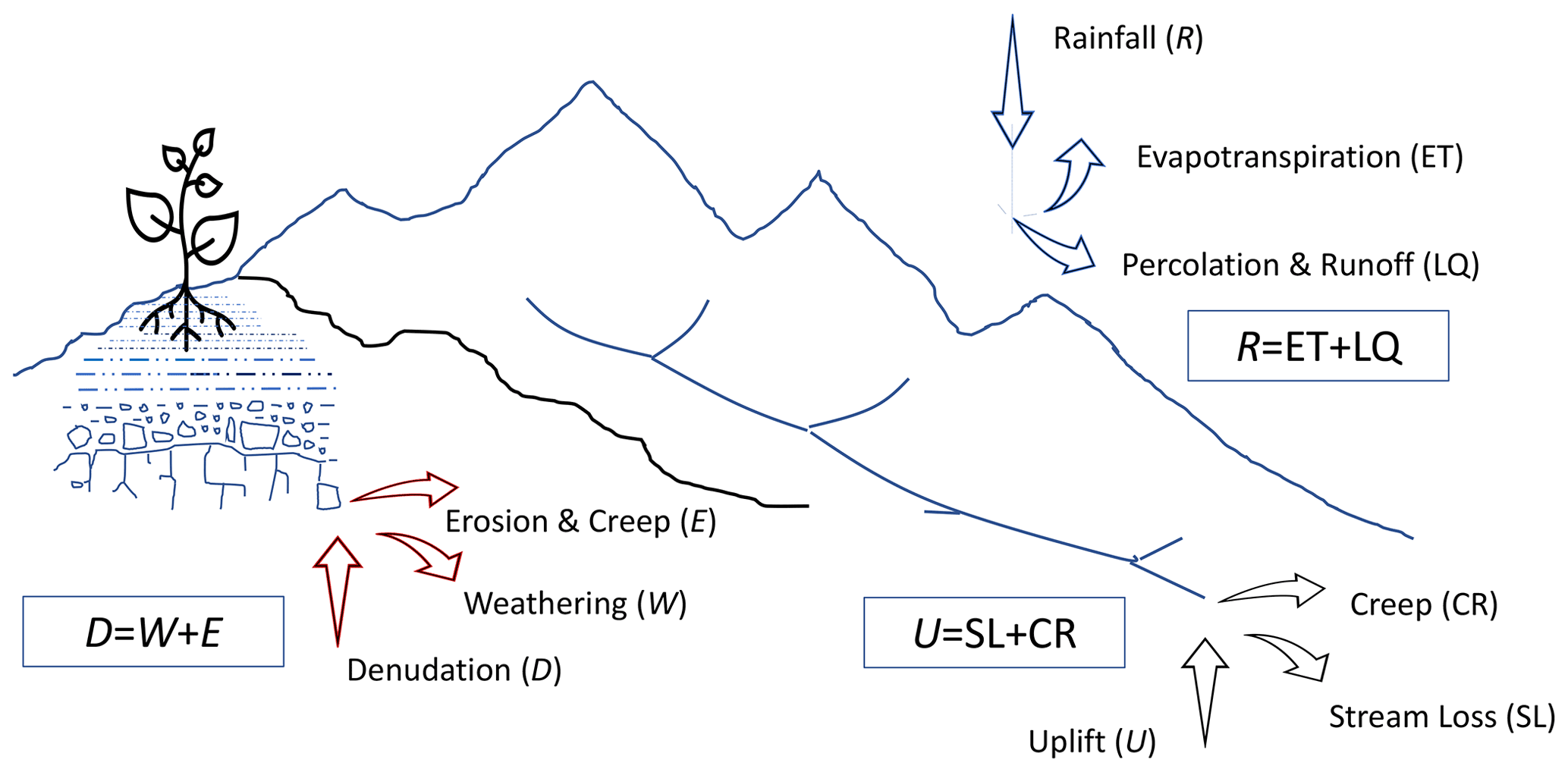
Figure 1 The three partitionings analyzed in this paper using dimensional analysis: the rainfall partitioning taking place at the land surface, the soil mineral partitioning by chemical dissolution (weathering) and transport processes, and the related partitioning of soil sediments responsible for landscape evolution and the formation of drainage networks.

The scaling laws obtained from dimensional analysis shed light on the dominant soil, vegetation and climate controls for these hydrologic partitionings. Specifically, in the first application it will be seen how the dimensionless dryness and storage indices determine the long-term rainfall partitioning. The second application will reveal the key nonlinear control of the dryness index on weathering rates, while the third application will analyze new macroscopic relations among average variables' landscape evolution, uncovering an intriguing analogy between self-similar topographies and turbulent flow fields.

3.1 Rainfall partitioning

The rainfall reaching the soil surface is either lost by runoff or infiltrates into the soil, where in turn it is lost either by evapotranspiration or percolation. The fate of this partitioning is essentially controlled by the properties of the soil–plant system, which – in a sense – acts as a geophysical valve, not only for the entire hydrologic cycle, but also for the energy and carbon cycles. This fundamental hydrological problem presents robust behaviors for its macroscopic (i.e., averaged) patterns as well as rich and complex controls at the detail level, where the role of temporal fluctuations and spatial heterogeneities becomes important.

We will indicate the mean rainfall rate as R and consider together the main losses: the evapotranspiration rate (ET) and the mean rate of percolation plus runoff (LQ); see Fig. 1. Assuming stationarity over long timescales and referring to a given area, the input balances the outputs:

$$\begin{array}{}\text{(8)}& R=\mathrm{ET}+\mathrm{LQ}.\end{array}$$

It should be clear that, depending on the area chosen and whether the latter is homogeneous in terms of land cover, soil properties, and topography, the actual meaning of the term LQ in Eq. (8) may be very different. In particular, if the control volume for our water balance is the rooting zone of a small homogeneous plot of vegetated soil, then LQ will be the average of a very intermittent term given by the sum of surface runoff and percolation to soil layers below the rooting zone, while if we consider an entire river basin, it will be mostly the average of the streamflow draining the area. How these processes scale with the land area is an interesting open question, which is outside of our scope (see Fig. 4 by Yin et al., 2019, for an analysis of this effect). We specifically focus on ET, as many have done before, but here we adopt the special lens offered by the Π theorem to explore the implications of different hypotheses in the physical laws used as starting points.

3.1.1 Turc and Budyko spaces: dryness and humidity as the main controls of rainfall partitioning

While they did not use dimensional analysis, Turc and Budyko started their work by making what is perhaps the simplest hypothesis of a physical law for the rainfall partitioning (see Dooge, 1992; Daly et al., 2019, and references therein),

$$\begin{array}{}\text{(9)}& \mathrm{ET}=f_{\mathrm{TB}}\left(R,{\mathrm{ET}}_{\max }\right),\end{array}$$

where ET_max is a reference (e.g., potential or maximum) evapotranspiration. The rank of the dimension matrix

$$\begin{array}{}\text{(10)}& \begin{array}{crrr}& \mathrm{ET}& R& {\mathrm{ET}}_{\max }\\ L& \mathrm{1}& \mathrm{1}& \mathrm{1}\\ T& -\mathrm{1}& -\mathrm{1}& -\mathrm{1}\end{array}\end{array}$$

is 1, which leads to a total of two dimensionless groups, one governed and one governing. Note that the same result is obtained adopting a system of units with the only dimension of flux, say Φ, for which the dimension matrix

$$\begin{array}{}\text{(11)}& \begin{array}{cccc}& \mathrm{ET}& R& {\mathrm{ET}}_{\max }\\ \mathrm{\Phi }& \mathrm{1}& \mathrm{1}& \mathrm{1}\end{array}\end{array}$$

also has rank 1.

If one chooses R as the repeating variable, applying the Π theorem then gives the so-called Budyko hypothesis

$$\begin{array}{}\text{(12)}& {\mathrm{\Pi }}_{\mathrm{B}}={\mathit{\phi }}_{\mathrm{B}}\left(D_{\mathrm{I}}\right),\end{array}$$

where

$$\begin{array}{}\text{(13)}& {\mathrm{\Pi }}_{\mathrm{B}}={\displaystyle \frac{\mathrm{ET}}{R}}\mathrm{and}{D}_{\mathrm{I}}={\displaystyle \frac{{\mathrm{ET}}_{\max }}{R}}\end{array}$$

is Budyko's dryness (or aridity) index. If instead one chooses ET_max, then Turc's hypothesis follows (Daly et al., 2019):

$$\begin{array}{}\text{(14)}& {\mathrm{\Pi }}_{\mathrm{T}}={\mathit{\phi }}_{\mathrm{T}}\left(H_{\mathrm{I}}\right),\end{array}$$

where

$$\begin{array}{}\text{(15)}& {\mathrm{\Pi }}_{\mathrm{T}}={\displaystyle \frac{\mathrm{ET}}{{\mathrm{ET}}_{\max }}}\mathrm{and}{H}_{\mathrm{I}}={\displaystyle \frac{R}{{\mathrm{ET}}_{\max }}}={\displaystyle \frac{\mathrm{1}}{D_{\mathrm{I}}}}\end{array}$$

is the humidity index. Which representation to use is mostly a matter of convenience, since they are related by ${\mathrm{\Pi }}_{\mathrm{T}}={\mathrm{\Pi }}_{\mathrm{B}}/D_{\mathrm{I}}$ and ${\mathit{\phi }}_{\mathrm{T}}={\mathit{\phi }}_{\mathrm{B}}/D_{\mathrm{I}}$. However, Budyko's hypothesis may be more suitable for emphasizing the dry end of the hydrologic spectrum, while Turc's privileges the humid end.

Budyko's hypothesis is tested in Fig. 2 using the MOPEX data for several river basins in the continental USA and plotted along with the original Budyko interpolating curve. Clearly, as shown many times before, the main controls on the rainfall partitioning are captured by the dryness index.

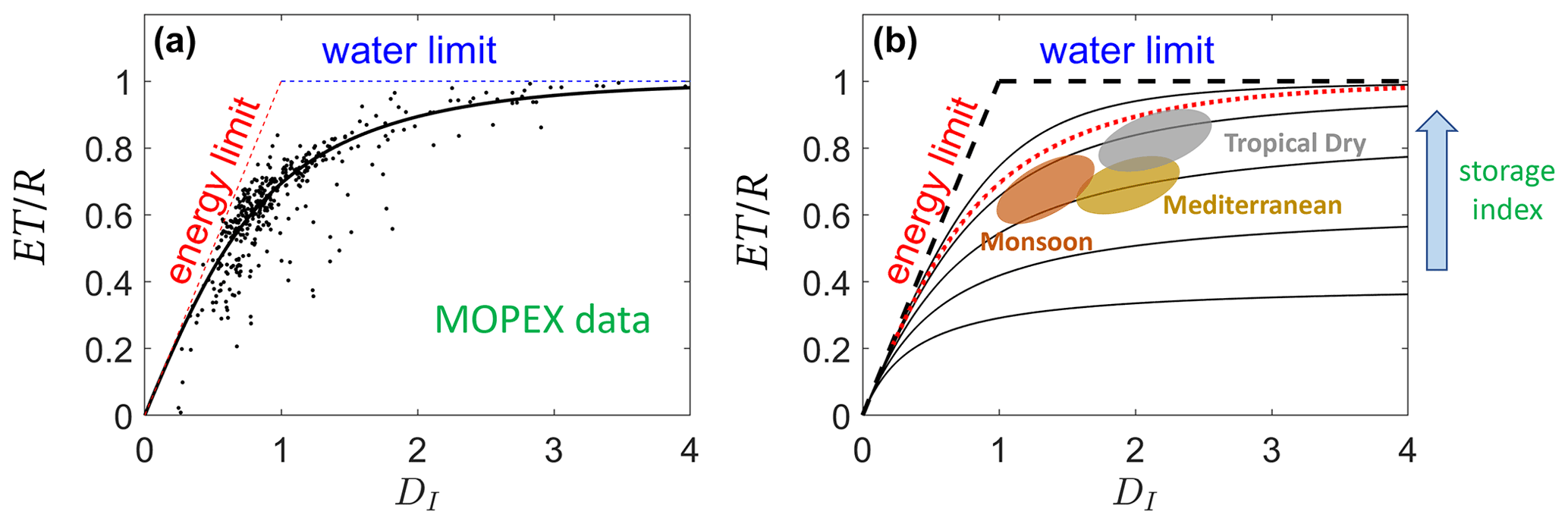
Figure 2 Rainfall partitioning. (a) Test of Budyko's hypothesis using the MOPEX data (Porporato and Yin, 2022). The solid line shows the original semi-empirical curve used by Budyko, ${\mathrm{\Pi }}_{\mathrm{B}}=\left(D_{\mathrm{I}}\tanh D_{\mathrm{I}}^{-\mathrm{1}}\right(\mathrm{1}-e^{-D_{\mathrm{I}}}){)}^{\mathrm{1}/\mathrm{2}}$. (b) Different solutions of the mean partitioning of the minimalist soil moisture balance model of Porporato et al. (2004), showing the role of the storage index, $\mathit{\gamma }=w_{\mathrm{0}}/\mathit{\alpha }$, and seasonality (Feng et al., 2012). The red dotted line is the original curve of Budyko.

3.1.2 Storage index: the role of the hydrologic active depth and the variability timescale

While the dryness index captures the main variability of the data, the scatter in Fig. 2 also suggests additional controls, which prompt us to revisit the physical law (Eq. 9) by considering additional governing quantities. There are several quantities that capture the different properties of the hydrologic system and its climatic forcing, such as storage capacity, areal extension, vegetation type, and seasonality. Among these candidates, the storage depth (the storage volume divided by the area) is probably the first one to consider, as suggested by the dramatic effects of paving a vegetated field on the rainfall partitioning.

To account for this effect, we may add a quantity w₀ with dimensions of length (L), which is a volume divided by an area. This leads to a physical law of the type

$$\begin{array}{}\text{(16)}& \mathrm{ET}=f_{\mathrm{ET}}\left(R,{\mathrm{ET}}_{\max },w_{\mathrm{0}}\right).\end{array}$$

However, when trying to apply the Π theorem, it becomes immediately apparent that, if w₀ is chosen as a repeating variable, it actually drops from the dimensionless formulation (similarly to the way the mass disappears from the list of variables when applying the Π theorem to the pendulum – Barenblatt, 1996). Physically, this tells us that to see a difference in the partitioning among the hydrologic balance of a parking lot, a crusted soil, and a deep vegetated soil, the role of the soil depth must be associated with other variables, which include a timescale to account for the variability of the hydrologic balance, for otherwise all the other influences are already contained in the dryness index.

Thus, to achieve a further refinement in the Pi-theorem formulation, in combination with the storage depth w₀, Porporato et al. (2004) introduced a timescale related to the mean time between rainfall events or – better – its inverse, the frequency of rainfall events, say λ. Since the frequency of rainfall times the mean rainfall depth per event α is equal to the mean rainfall rate R=αλ, the presence of the mean rainfall rate in the list becomes redundant if one already includes the mean rainfall depth α. With these additions, the physical law becomes

$$\begin{array}{}\text{(17)}& \mathrm{ET}=f_{\mathrm{ET}}\left(\mathit{\lambda },\mathit{\alpha },{\mathrm{ET}}_{\max },w_{\mathrm{0}}\right),\end{array}$$

with the dimension matrix of rank 2 given by

$$\begin{array}{}\text{(18)}& \begin{array}{crrcrc}& \mathrm{ET}& \mathit{\lambda }& \mathit{\alpha }& {\mathrm{ET}}_{\max }& w_{\mathrm{0}}\\ L& \mathrm{1}& \mathrm{0}& \mathrm{1}& \mathrm{1}& \mathrm{1}\\ T& -\mathrm{1}& -\mathrm{1}& \mathrm{0}& -\mathrm{1}& \mathrm{0}\end{array}.\end{array}$$

It is instructive to explore the full range of choices related to the three possible dimensionless groups given by the five variables minus the rank 2 of the matrix. In turn, this implies five possibilities (of the six potential pairs of repeating variables, (α, w₀) obviously must be excluded because of dimensional dependence), which can all be brought back to the dryness index D_I and the storage index $\mathit{\gamma }=w_{\mathrm{0}}/\mathit{\alpha }$, as shown in the following table:

$$\begin{array}{}\text{(19)}& \begin{array}{lll}\mathrm{Repeating}\mathrm{var}.& \mathrm{Pi}\mathrm{theorem}& \mathrm{Group}\mathrm{relation}\\ (\mathit{\alpha },\mathit{\lambda })& \frac{\mathrm{ET}}{\mathit{\alpha }\mathit{\lambda }}={\mathit{\phi }}_{\mathrm{1}}\left(\frac{E_{\max }}{\mathit{\alpha }\mathit{\lambda }},\frac{w_{\mathrm{0}}}{\mathit{\alpha }}\right)& {\mathrm{\Pi }}_{\mathrm{B}}={\mathit{\phi }}_{\mathrm{1}}\left(D_{\mathrm{I}},\mathit{\gamma }\right)\\ \left(\mathit{\lambda },E_{\max }\right)& \frac{\mathrm{ET}}{E_{\max }}={\mathit{\phi }}_{\mathrm{2}}\left(\frac{\mathit{\alpha }\mathit{\lambda }}{E_{\max }},\frac{w_{\mathrm{0}}\mathit{\lambda }}{E_{\max }}\right)& {\mathrm{\Pi }}_{\mathrm{B}}{D}_{\mathrm{I}}^{-\mathrm{1}}={\mathit{\phi }}_{\mathrm{2}}\left(D_{\mathrm{I}}^{-\mathrm{1}},\mathit{\gamma }{D}_{\mathrm{I}}^{-\mathrm{1}}\right)\\ \left(\mathit{\alpha },E_{\max }\right)& \frac{\mathrm{ET}}{E_{\max }}={\mathit{\phi }}_{\mathrm{3}}\left(\frac{E_{\max }}{\mathit{\alpha }\mathit{\lambda }},\frac{w_{\mathrm{0}}}{\mathit{\alpha }}\right)& {\mathrm{\Pi }}_{\mathrm{B}}{D}_{\mathrm{I}}^{-\mathrm{1}}={\mathit{\phi }}_{\mathrm{3}}\left(D_{\mathrm{I}}^{-\mathrm{1}},\mathit{\gamma }\right)\\ \left(\mathit{\lambda },w_{\mathrm{0}}\right)& \frac{\mathrm{ET}}{\mathit{\lambda }{w}_{\mathrm{0}}}={\mathit{\phi }}_{\mathrm{4}}\left(\frac{E_{\max }}{\mathit{\lambda }{w}_{\mathrm{0}}},\frac{\mathit{\alpha }}{w_{\mathrm{0}}}\right)& {\mathrm{\Pi }}_{\mathrm{B}}{\mathit{\gamma }}^{-\mathrm{1}}={\mathit{\phi }}_{\mathrm{4}}\left(D_{\mathrm{I}}{\mathit{\gamma }}^{-\mathrm{1}},{\mathit{\gamma }}^{-\mathrm{1}}\right)\\ \left(E_{\max },w_{\mathrm{0}}\right)& \frac{\mathrm{ET}}{E_{\max }}={\mathit{\phi }}_{\mathrm{5}}\left(\frac{\mathit{\alpha }}{w_{\mathrm{0}}},\frac{\mathit{\lambda }{w}_{\mathrm{0}}}{E_{\max }}\right)& {\mathrm{\Pi }}_{\mathrm{B}}{D}_{\mathrm{I}}^{-\mathrm{1}}={\mathit{\phi }}_{\mathrm{5}}\left({\mathit{\gamma }}^{-\mathrm{1}},\mathit{\gamma }{D}_{\mathrm{I}}^{-\mathrm{1}}\right)\end{array}.\end{array}$$

These five hydrologic spaces provide different, if related, scaling laws that allow us to focus on the role of specific combinations of parameters and emphasize different hydrologic conditions. It is useful to note that the dimensionless group $\mathit{\vartheta }=\mathit{\gamma }{D}_{\mathrm{I}}^{-\mathrm{1}}=\frac{\mathit{\lambda }{w}_{\mathrm{0}}}{E_{{\mathrm{ET}}_{\max }}}$ appears often as an independent variable. The latter can also be written as $\mathit{\vartheta }=\frac{\mathit{\lambda }}{\mathit{\eta }}$, which uncovers an interpretation of it as a ratio of timescales, one related to the mean time between rainfall occurrence, $\mathrm{1}/\mathit{\lambda }$, and one related to the time of depletion of the soil store reservoir of depth w₀ at the maximum evapotranspiration rate, i.e., $\mathit{\eta }=E_{\max }/w_{\mathrm{0}}$. Note also that $\mathit{\vartheta }=\frac{\mathit{\lambda }}{\mathit{\eta }}$ appears naturally in the normalized form of the evolution equation of the probability distributions of soil moisture dynamics in minimalist stochastic models (Porporato et al., 2004; Rodríguez-Iturbe and Porporato, 2005). Figure 2b reports different partitioning curves for different values of the storage index γ, obtained by solving a minimalist stochastic soil moisture model with only four dimensional parameters as in Eq. (17).

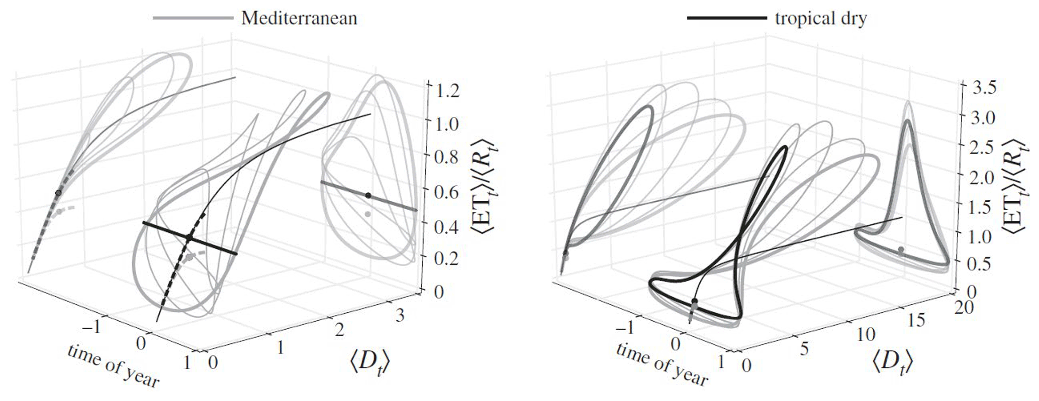
Figure 3 Transient trajectories of the time-varying ratio $\langle {\mathrm{ET}}_t\rangle /\langle R_t\rangle$ as a function of the time-varying dryness index 〈D_t〉 and time of year for Mediterranean and tropical dry climates. Brackets indicate ensemble averages for a given time of year, taken over the rainfall variability due to a time-dependent (i.e., seasonal) marked Poisson process of rainfall and seasonal potential evapotranspiration. Each loop is derived from the same climate inputs, with the exception of the phase difference between rainfall and potential evapotranspiration, with the thick grey lines showing results for out-of-phase and thick black lines for in-phase. The +1 on the time-of-year axis corresponds to when maximum rainfall occurs (wet season), and −1 corresponds to timing of minimum rainfall (dry season). The annual average value for each loop falls on a single point on the annual Budyko curves, shown as dashed lines (black and grey) for those that account for climate seasonality and as thin black lines for the classical curve which considers only annually averaged climate values. After Feng et al. (2015).

With the goal of analyzing the suitability of different hydrologic spaces for capturing the information available in global datasets on hydrologic partitioning, Daly et al. (2019) analyzed a physical law focused on hydrologic fluxes (i.e., rates) only. Accordingly, they considered an extension of Budyko and Turc physical laws (Eq. 9) by hypothesizing an additional control by a governing variable ϕ with the dimensions of a flux, $\left[\mathit{\varphi }\right]=L{T}^{-\mathrm{1}}=\mathrm{\Phi }$,

$$\begin{array}{}\text{(20)}& \mathrm{ET}=f_{\mathrm{ET}}\left(R,{\mathrm{ET}}_{\max },\mathit{\varphi }\right).\end{array}$$

Since each of the fluxes ($L/T=\mathrm{\Phi }$) can be used as a repeating variable, three hydrologic spaces are obtained. Assuming further that ϕ is a flux related to the storage capacity and the frequency of rainfall, ϕ=λw₀, the three spaces (Daly et al., 2019) are found to coincide with specific cases in Eq. (19): case 1 if R is chosen as a repeating variable, case 2 if ET_max is chosen, and case 4 if ϕ is chosen.

The analysis by Daly et al. (2019) shows that by accounting for the ability of a catchment to store water to supply evapotranspiration, the flux ϕ (referred to as the maximum storage rate) serves as a modulator for the relationships of ET with R and ET_max for very dry and very wet catchments. In this way, accounting for it, it allows us to expand the Budyko and Turc frameworks, suggesting that they are not equivalent, as often assumed in parametric models, unless ϕ→∞. Thus the variable ϕ helps group catchments with similar evapotranspiration rates with respect to different combinations of the dimensionless groups $\mathit{\varphi }/{\mathrm{ET}}_{\max }=\left(\mathit{\lambda }{w}_{\mathrm{0}}\right)/{\mathrm{ET}}_{\max }=\mathit{\vartheta }=\mathit{\gamma }{D}_{\mathrm{I}}^{-\mathrm{1}}$ and $\mathit{\varphi }/R=w_{\mathrm{0}}/\mathit{\lambda }=\mathit{\gamma }$, which account for key catchment and hydrologic characteristics. It also facilitates the analysis of the partitioning in catchments with intermediate values of the dryness index, while Budyko's and Turc's hypotheses help in the analysis of very dry and wet catchments, respectively (Daly et al., 2019).

3.1.3 Seasonality, variable coevolution, and higher-order effects

It is logical to wonder about the effects of adding other potentially important variables to the physical law of rainfall partitioning. These could include variables describing seasonality, soil and vegetation properties, and other details of the climatic forcing. With the goal of investigating the role of seasonality in rainfall and evapotranspiration, Feng et al. (2012) considered the duration of the wet season and the intensity of rainfall seasonality. The effect of the new dimensionless groups obtained on the long-term partitioning is shown in Fig. 2b. Depending on the degree and type of seasonality, a reduction of evapotranspiration is typically observed due to an increase in percolation during the wet season compared to the homogeneous case with no seasonality. At the level of approximation afforded by the long-term averaging, the effects of seasonality are hardly distinguishable from those of a decrease in the storage index γ. To disentangle the various effects and more clearly see the effects of seasonality, the temporal variability in the rainfall partitioning must be considered. An example of this is presented in Fig. 3, where the Budyko curve is plotted parametrically as a function of time and the non-uniqueness related to seasonal storage becomes evident (Feng et al., 2015).

It is clear that more detailed analyses to disentangle the role of different ecohydrological variables in the rainfall partitioning should focus on specific aspects of the space–time variability of evapotranspiration, which instead are lost in the spatially lumped, long-term evapotranspiration rates of Budyko's type analyses. The combination with simple physically based models may be a valuable way to sharpen the hypotheses of the physical laws, especially when trying to unravel the effects of the covariation of some of the variables. These regard questions of how the rooting depth, and thus the storage capacity of the active soil layer, may depend on the dryness index and whether such covariations may imply some adaptation of vegetation and soil properties to the hydroclimatic characteristics. Along these lines, the minimalist stochastic model developed by Porporato et al. (2004) pointed to a tendency, for the points lying on the Budyko curve, to converge towards typical values of the storage index of 5–6, in turn suggesting a root-depth adaptation to the intensity of rainfall. Similarly, Or and Lehmann (2019) attributed the convergence of the rainfall partitioning to typical evaporative depths, while Hunt (2021) connected a dependence of the storage index with hydroclimatic characteristics, γ(D_I), to an adaptation brought about by constraints linked to percolation statistics.

Shedding light on the role of higher-order controls in rainfall partitioning requires charting of more detailed model–data investigations, branching off the beaten path of Budyko-type analyses. Long-term averages may only contain a weak signal of those interactions, which may be easily overwhelmed by noise and other data limitations. This suggests a need for adapting dimensional analysis to these other aspects of the rainfall partitioning and formulating more sophisticated physical laws that capture the more subtle controls by the soil–plant–atmosphere system (see Feng et al., 2018, for an example).

3.2 Soil formation, weathering, and loss

A partitioning of the soil mineral component also takes place, on much larger timescales, on the land surface (Riebe et al., 2004). The loss of minerals at the land surface is controlled by a series of tightly connected chemico-physical processes with interesting geomorphology and hydrologic interactions (Maher and Chamberlain, 2014), which in turn have a crucial impact on the surface energy and water balances as well as several biogeochemical, ecological, and climate processes (Garrels, 1983; Richter and Billings, 2015).

The input of solid material to the soil from breaking up parent rock is called rock denudation. While the dissolved minerals and the very fine particles resulting from denudation can be transported away by water, the remaining particles stay in the ground, where they continue to be weathered until they too can be transported away. As the soil ages and transforms chemically, the soil may also be deformed by the action of internal stresses and move as creeping flow. As a result, if one assumes, for simplicity, that the input and output balance (Riebe et al., 2004), denudation D equals soil formation rate. These in turn balance the losses by weathering W and erosion plus creep, which are lumped here into a single term E (Fig. 1), yielding the following soil partitioning:

$$\begin{array}{}\text{(21)}& D=W+E.\end{array}$$

To analyze this partitioning and help resolve the complex interaction between chemical weathering, climate, and the hydrologic cycle, Calabrese and Porporato (2020) used dimensional analysis. This allowed them to obtain a theoretical framework to organize the existing data on weathering rates. Because of the crucial role of leaching of dissolved inorganic carbon on the sites of weathering, the problem strongly depends on the rainfall partitioning at the surface discussed in the previous section. Accordingly, focusing on the weathering rate as the governed quantity, Calabrese and Porporato (2020) wrote a physical law assuming that weathering rates are a function of the input given by the denudation rate, a maximum weathering rate (which includes the effects of type of parent material, temperature, etc.), the concentration of dissolved inorganic carbon [DIC], and the percolation flux LQ (see Eq. 3). Further assuming that both [DIC] and LQ only depend on the surface rainfall partitioning through the dryness index, as in Budyko's hypothesis (Eq. 12), they wrote

$$\begin{array}{}\text{(22)}& W=f_{\mathrm{W}}\left(D,W_{\max },D_{\mathrm{I}}\right).\end{array}$$

Formally, apart from the presence of the dimensionless dryness index, the situation is similar to the one of Eq. (3), since W, D, and W_max all have the same dimensions of a flux of mineral per time. Choosing the input D as the repeating variable in Eq. (21), as Budyko did in the rainfall partitioning, the Π theorem gives

$$\begin{array}{}\text{(23)}& {\displaystyle \frac{W}{D}}={\mathit{\phi }}_{\mathrm{W}}\left({\displaystyle \frac{W_{\max }}{D}},D_{\mathrm{I}}\right).\end{array}$$

To verify this functional relationship, Calabrese and Porporato (2020) used literature data including granitic, basaltic, and shale terrains and encompassing a broad range of environmental settings. After normalizing the data by their maximum rate and assuming for the range of data available that W≤D, the results (Fig. 4a) show a remarkable linear trend of the type

$$\begin{array}{}\text{(24)}& {\displaystyle \frac{W}{D}}={\left({\displaystyle \frac{W_{\max }}{D}}\right)}^m{\mathit{\psi }}_{\mathrm{W}}\left(D_{\mathrm{I}}\right).\end{array}$$

Since the exponent m of the power law is very close to 1, the expression can be further simplified to the final form

$$\begin{array}{}\text{(25)}& {\displaystyle \frac{W}{W_{\max }}}={\mathit{\psi }}_{\mathrm{W}}\left(D_{\mathrm{I}}\right).\end{array}$$

Figure 4 (a) Analysis of the self-similarity hypothesis in Eq. (24); (b) specific weathering rates as a function of the dryness index; dashed line shows Eq. (26). After Calabrese and Porporato (2020).

Both these expressions are suggestive of self-similarity. At a first glance, looking at Eq. (24), one would be led to conclude that we are in the presence of self-similarity of the second type with respect to $W_{\max }/D$. However, an exponent practically equal to one, unlike the typical irrational numbers expected in incomplete self-similarity (Barenblatt, 1996), leads to a simplification which eliminates the governing variable D. As a result, the final expression (Eq. 25) can be interpreted as a case of complete self-similarity with respect to $D/W_{\max }$, when W_max is chosen as a repeating variable in Eq. (22) instead of D. Alternatively, the same expression can be obtained directly from the Π theorem starting from an abbreviated physical law $W=f_{W_a}(W_{\max },D_{\mathrm{I}})$. The precise meaning of this self-similarity remains an open problem to be investigated. The physical message however is that the denudation rate is not a relevant quantity compared to the maximum weathering.

Equation (25) provides a mathematical structure to analyze how the water cycle affects the chemical depletion fraction through the dryness index. The empirical data fit provides an equation with only one parameter,

$$\begin{array}{}\text{(26)}& {\mathit{\psi }}_{\mathrm{W}}\left(D_{\mathrm{I}}\right)=\mathrm{1}-{\displaystyle \frac{\ln \left(D_{\mathrm{I}}^{\mathit{\alpha }}+\mathrm{1}\right)}{\mathrm{1}+\ln \left(D_{\mathrm{I}}^{\mathit{\alpha }}+\mathrm{1}\right)}},\end{array}$$

which emphasizes the strongly nonlinear relation between water availability and weathering rate (see Fig. 4b). Starting from high D_I values, the normalized weathering rate increases only slightly up until D_I∼2, after which it steeply increases before plateauing at D_I∼0.5. The increase region corresponds to the establishment of grassland, savanna, and shrubland ecosystems, emphasizing the important role of vegetation in acidifying the soil and in turn enhancing weathering rates. A similar nonlinear dependence on wetness has been observed in the global distribution of soil organic carbon (Kramer and Chadwick, 2018).

The scatter shown by the data in Fig. 4b is not unexpected, because of the large datasets used, which are obtained from different locations and different methods. While it is likely that part of it may be attributable to noise, it would also be interesting to consider whether adding other quantities in the physical law might help explain more of this variability. A logical starting point could be the analysis of the effects of the soil depth and water-storage capacity, which could be explored by correlating the data with estimates of the storage index γ. It is likely that this will reveal further linkages between surface hydrology, soil formation, and weathering.

3.3 Landscape self-similarity

Besides the macroscopic effects of wetness on weathering discussed in the previous section, the loss of minerals driven by the coupled water and sediment fluxes on the topographic surface is also responsible for the formation of complex topographic patterns, which in turn impact ecohydrologic processes (Dietrich and Perron, 2006). In this section, we focus on the dendritic morphology of interlocked ridges and valleys, which often displays a self-similar scaling linked to the fractal behavior of landscapes (Rodríguez-Iturbe and Rinaldo, 2001). While on the one hand the complexity of these patterns hinders analytical results, on the other hand it also helps with the investigation of macroscopic (i.e., averaged) behavior, giving rise, as we will see, to emergent scaling behaviors for the large-scale statistics of the sediment budget, the mean elevation profile, and the landscape spectral properties.

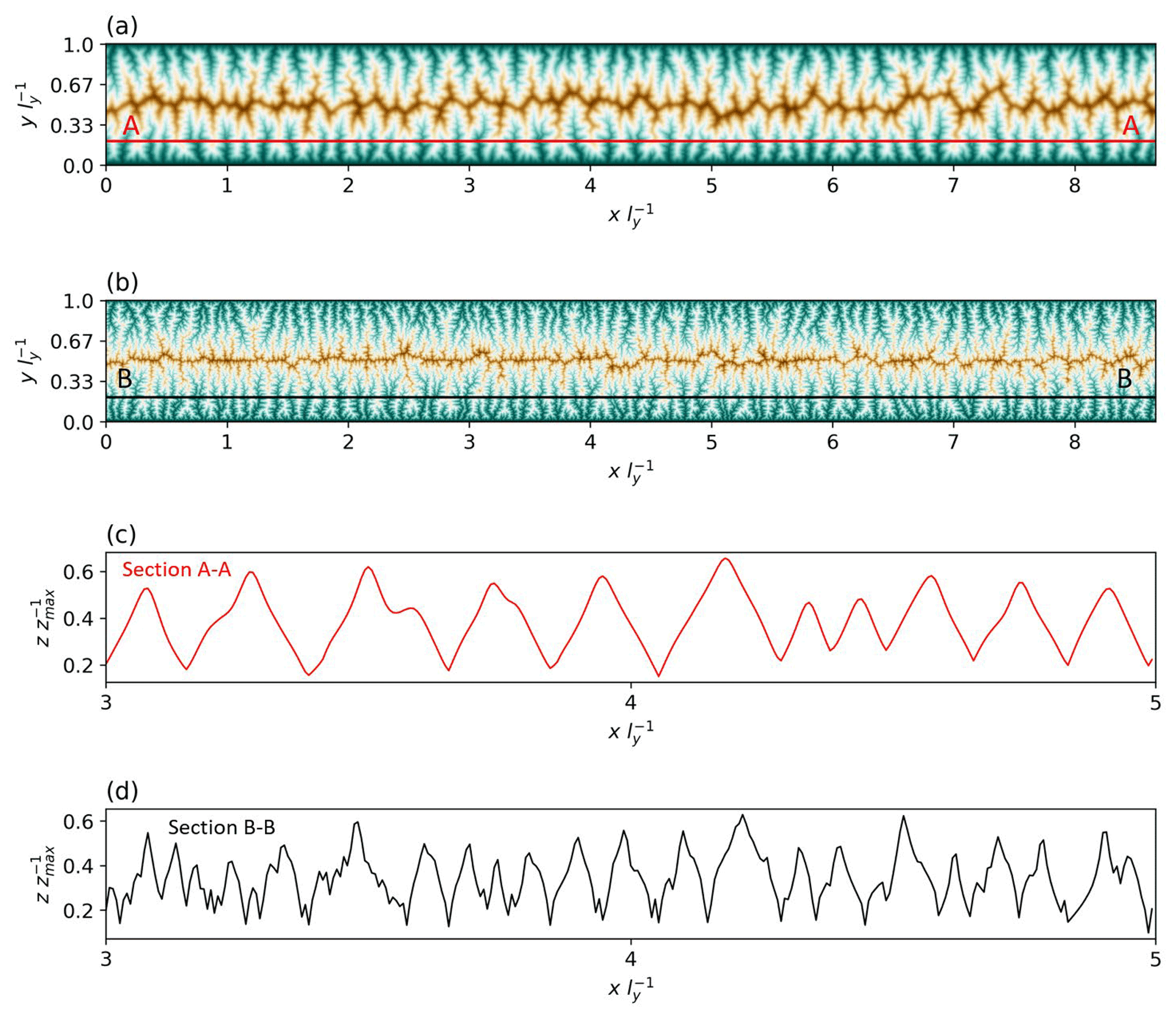
Figure 5 Steady-state simulation of landscape elevation given by Eqs. (27) and (28) for m=0.5 and different channelization indices, Eq. (33), 𝒞_I=10³ in (a) and 𝒞_I=10⁴ in (b). The elevation along A–A and B–B transects is shown in (c) and (d). After Hooshyar et al. (2021).

Towards the goal of performing dimensional and self-similarity analyses, here we will consider only (spatially) averaged quantities in idealized geometries for which the solutions may be expected to depend only on a limited number of dimensionless quantities. The effort of formulating meaningful physical laws for average landscape quantities is facilitated by the existence of simplified, semi-empirical landscape evolution models (LEMs) (Chen et al., 2014), which can be inspected to infer the main governing quantities of the problems. We specifically refer to a minimalist landscape evolution model in detachment-limited conditions (Howard, 1994), although many considerations also apply to transport-limited and other intermediate formulations (Davy and Lague, 2009; Pelletier, 2012). Accordingly, the equation for the evolution of the landscape elevation $z(x,y,t)$ is (Chen et al., 2014)

$$\begin{array}{}\text{(27)}& {\displaystyle \frac{\partial z}{\partial t}}=\mathit{\delta }{\mathrm{\nabla }}^{\mathrm{2}}z-K{a}^m\left|\mathrm{\nabla }z\right|+U,\end{array}$$

where t is time, δ is the diffusion coefficient used to represent the intensity of soil creep, K is the fluvial erosion coefficient, $a(x,y,t)$ is the specific drainage area, m is a dimensionless coefficient (for simplicity we assume the exponent of the gradient in the erosion term to be equal to 1), and U is the surface-growth term due to tectonic uplift. Equation (27) is coupled to the “conservation” equation for the specific drainage area:

$$\begin{array}{}\text{(28)}& \mathrm{\nabla }\cdot \left(a{\displaystyle \frac{\mathrm{\nabla }z}{\left|\mathrm{\nabla }z\right|}}\right)=\mathrm{1}.\end{array}$$

The latter was derived by Bonetti et al. (2018) as an idealized representation of the water flow, following the steepest descent lines of a topographic surface with a given characteristic speed (see also Bonetti et al., 2020). Mathematically, $a=\underset{w\to \mathrm{0}}{lim}A/w$, where A is the contributing area and w is a finite portion of a contour (iso-elevation); hence, the specific drainage area has dimensions of length, [a]=L, and is defined at a point on the landscape, whereas the contributing area A, [A]=L², is actually zero when considered at a point, unless the topographic surface is discontinuous (see Bonetti et al., 2018, for details). The use of the nonlocal quantity A instead of a in Eq. (27) is therefore incorrect and leads to grid-dependent results in mathematical codes. Since the equation of a is not very well known, and given the misuse of A in the literature, we present a short derivation of Eq. (28) in Appendix B.

The coupled Eqs. (27) and (28) form a closed system once the initial and boundary conditions are specified. Figure 5 shows simulation results producing complex patterns (Anand et al., 2020) that resemble real landscapes, with characteristic branching and channelization instability. A dimensional analysis of terms in a LEM in detachment-limited conditions was presented by Theodoratos et al. (2018), although they use A instead of a in the evolution equation for h. Throughout this section, we will also see how the statistics of landscape elevation bear a striking resemblance to those of streamwise velocity in near-wall turbulence (Hooshyar et al., 2020). For comparison, Appendix C briefly reports the Navier–Stokes equations for the case of channel flow between two parallel plates, which corresponds to the case of the landscape evolution between two parallel boundaries at fixed elevation (e.g., Fig. 5).

3.3.1 Sediment budget and soil partitioning

In steady state, spatial averaging leads to the partitioning of soil material into soil creep (SC) and the soil loss by stream erosion (SL),

$$\begin{array}{}\text{(29)}& U=\mathrm{CR}+\mathrm{SL}.\end{array}$$

This equation is obviously related to Eq. (21), since at steady state the rate of uplift needs to equal the denudation rate, while the losses may be grouped by focusing on different features of the underlying processes. Equation (21) emphasizes chemical weathering while lumping all the other losses (mainly erosion and creep) into the term E, while here Eq. (29) draws attention to the water-erosion term SL (possibly including also weathering), with the rest lumped into a diffusive term, CR, representing soil creep and other smoothing processes.

Averaging spatially Eqs. (27) and (28), the mean sediment balance equation can be written as (see Hooshyar and Porporato, 2021, for details)

$$\begin{array}{}\text{(30)}& \underset{-\mathrm{CR}}{\underbrace{\mathit{\delta }{\left(\mathrm{2}{l}_y\right)}^{-\mathrm{1}}{〈\mathrm{\nabla }{z}_{⟂}〉}_{\mathrm{\Omega }}}}-\underset{\mathrm{SL}}{\underbrace{K\left((\mathrm{1}-m)〈{\mathit{\kappa }}_{\mathrm{c}}{a}^{m}z〉+m〈a^{m-\mathrm{1}}z〉\right)}}+U=\mathrm{0},\end{array}$$

where l_y is the domain width, ∇z_⟂ is the component of the elevation gradient normal to the domain contour Ω, κ_c is the plane or contour curvature, the brackets 〈⋅〉 indicate the spatial average, and 〈⋅〉_Ω is the average over the domain contour. While this is an exact result, the terms in brackets are unknown because of the complexity of the landscape surface. This is where dimensional analysis comes in handy.

Bonetti et al. (2020) tackled the problem of these spatial averages by adopting a directional dimensional analysis (see Sect. 2.3), considering independent dimensions for horizontal lengths, L, and the vertical length, L_z. Physically, a justification for the use of directional dimensional analysis may be found in the fact that Eq. (27) is the sediment budget equation at a point written in terms of volume of sediments per unit ground area. For sediments of constant density, the same equation can be written in terms of mass per unit ground area, say ρz, which then can be considered a new variable with its independent dimensions. Indicating the unknown average slope at the boundary as $S_{*}=\langle \mathrm{\nabla }{z}_{⟂}{\rangle }_{\mathrm{\Omega }}$, the physical law can be written as

$$\begin{array}{}\text{(31)}& S_{*}=f\left(l_y,K,U;\mathit{\delta },m\right),\end{array}$$

where the various quantities are suggested by inspection of the governing equations and the type of boundary conditions. For this problem, $\left[S_{*}\right]=L_z{L}^{-\mathrm{1}}$, $\left[U\right]=L_z{T}^{-\mathrm{1}}$, $\left[\mathit{\delta }\right]=L^{\mathrm{2}}{T}^{-\mathrm{1}}$, $\left[K\right]=L^{\mathrm{1}-m}{T}^{-\mathrm{1}}$, and [m]=1. Choosing l_y, K, and U as repeating variables, the Π theorem then yields

$$\begin{array}{}\text{(32)}& {\displaystyle \frac{\mathit{\delta }{S}_{*}}{U{l}_y}}={\displaystyle \frac{\mathrm{2}\mathrm{CR}}{U}}={\mathit{\phi }}_{\mathrm{CR}}\left(C_{\mathrm{I}}^{-\mathrm{1}},m\right)={\mathit{\psi }}_{\mathrm{CR}}\left(C_{\mathrm{I}},m\right),\end{array}$$

where

$$\begin{array}{}\text{(33)}& C_{\mathrm{I}}={\displaystyle \frac{K{l}^{m+\mathrm{1}}}{\mathit{\delta }}}\end{array}$$

is the global channelization index. Figure 6 shows the plot of the function (Eq. 32) obtained from a set of simulations with different C_I and m values.

These results suggest a tantalizing analogy with the analysis of wall-bounded turbulent shear flows. In fact, the regular behavior of φ(C_I,m) reminds one of the behavior of the Darcy friction factor plotted in the Moody diagram for pipe flow (Munson et al., 2013). For a detailed description of dimensional analysis in turbulence, see Barenblatt (1996) and Katul et al. (2019). In this analogy, the slope of the elevation profile and the slope of the velocity profile play a similar role. As is well known, in turbulence, the mean velocity profile at the wall is proportional to the wall shear stress and relates to the partitioning of viscous and turbulent stresses; this is analogous here to the partitioning of soil coming from uplift into creep and stream erosion – see Eq. (30). We will highlight further links with the dimensional analysis of wall-bounded turbulent flows in the subsequent developments.

It is also useful to note that in Bonetti et al. (2020) the Π theorem was applied to Eq. (31) considering l_y, U, and δ to be repeating variables, which instead leads to Π_δ=φ_δ(C_I), with Π_δ=Π_CRC_I and ${\mathit{\phi }}_{\mathit{\delta }}\left(C_{\mathrm{I}}\right)={\mathit{\psi }}_{\mathrm{CR}}\left(C_{\mathrm{I}}\right)C_{\mathrm{I}}^{-\mathrm{1}}$. In the turbulence analogy, the present analysis corresponds to choosing viscosity instead of density (which is the typical choice; see Katul et al., 2019) as one of the repeating variables in the physical law for the wall-shear stress. Thus, for the wall-shear stress, $\mathit{\tau }=\mathit{\mu }{\mathrm{\Sigma }}_{*}$, where μ is the dynamic viscosity and Σ_* is the slope of the streamwise velocity profile at the wall, the physical law is $\mathit{\tau }=f_{\mathit{\tau }}(V,L,\mathit{\rho },\mathit{\mu },\mathit{ϵ})$, where ρ is the density, V the mean velocity, L the characteristic lateral dimension, and ϵ the roughness height. Using V, L, and μ as repeating variables, one has $\frac{\mathit{\tau }L}{\mathit{\mu }V}=Re\cdot \frac{\mathit{\tau }}{\mathit{\rho }{V}^{\mathrm{2}}}=Re\cdot f_{\mathrm{Darcy}}\left(Re,\frac{\mathit{ϵ}}{L}\right)$, where $Re=\frac{\mathit{\rho }VL}{\mathit{\mu }}$ is the bulk Reynolds number.

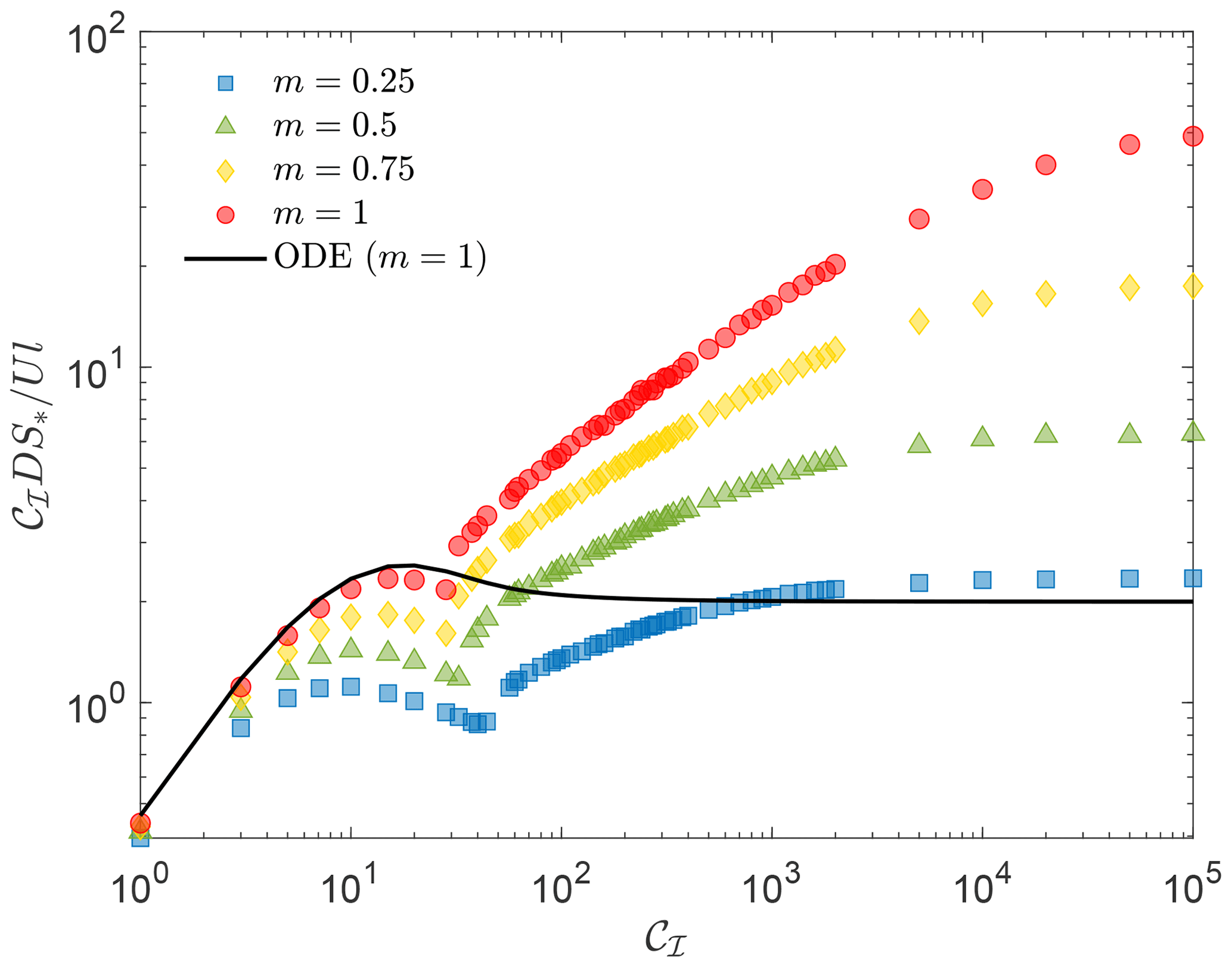
Figure 6 Average sediment partitioning according to Eq. (32) as a function of the channelization index for different values of m. Points refer to numerical simulations and solid line refers to the analytical solution for the unchannelized regime (courtesy of Sara Bonetti).

A second interesting fact is the plateauing of the curves at large values of C_I for both the analytical solution in the unchannelized case and the numerical results in the channelized regime. This suggests the existence of complete self-similarity for C_I→∞, again analogous to the self-similarity observed in the Moody diagram for the friction factor in the fully rough regime (Munson et al., 2013). Thus, while erosion dominates over creep, the effect of diffusion does not fully disappear but remains present, probably concentrated in an area of zero measure corresponding to the network of ridges and valleys. Again, this singular limit bears similarities to the much investigated limit of the viscous Navier–Stokes equations for Reynolds numbers tending to infinity as well as the hypothesis of dissipative anomalies in the inviscid Euler equations (e.g., Eyink, 2008).

3.3.2 Mean elevation profile

Hooshyar et al. (2020) analyzed the profile of the mean elevation, $\stackrel{\mathrm{‾}}{z}\left(y\right)={lim}_{l_x\to \mathrm{\infty }}\frac{\mathrm{1}}{l_x}\underset{\mathrm{0}}{\overset{l_x}{\int }}z(x,y)\mathrm{d}x$, of channelized landscapes. Based on the inspection of the governing equations and again using directional dimensional analysis, the physical law for the slope of the profile was assumed to be

$$\begin{array}{}\text{(34)}& {\displaystyle \frac{\mathrm{d}\stackrel{\mathrm{‾}}{z}}{\mathrm{d}y}}=f_{\frac{\mathrm{d}\stackrel{\mathrm{‾}}{z}}{\mathrm{d}y}}\left(y,\mathit{\delta },z_{*};l_y,K,U,m\right),\end{array}$$

where y is the distance from the boundary and z_* is an elevation scale. Choosing y, δ, and z_* as repeating variables and with simple manipulation of the dimensionless groups, the Π theorem gives

$$\begin{array}{}\text{(35)}& (m+\mathrm{1})\mathit{\eta }{\displaystyle \frac{\mathrm{d}\mathit{\phi }}{\mathrm{d}\mathit{\eta }}}=f_{\mathrm{3}}\left(\mathit{\eta },{\mathcal{C}}_{\mathrm{I}},\mathit{\zeta },m\right),\end{array}$$

where $\mathit{\phi }=\frac{\stackrel{\mathrm{‾}}{z}}{z_{*}}$. In addition to the global channelization index, C_I, reflecting the relative impact of fluvial erosion to diffusive transport, $\mathit{\eta }=\frac{K{y}^{m+\mathrm{1}}}{\mathit{\delta }}$ is a local variable with a similar form to 𝒞_I but capturing the local relative contribution of those two processes, while $\mathit{\zeta }=\frac{U{l}_y^{\mathrm{2}}}{\mathit{\delta }{z}_{*}}$ describes the relative impact of tectonic uplift on diffusive transport.

In a system with relatively small diffusive transport and dominated by erosion and uplift, 𝒞_I and ζ take high values. The same argument also applies to η except for locations at an intermediate distance from the boundary. Thus, when the variables η, 𝒞_I, and ζ reach such an asymptotic condition, one may assume complete self-similarity (Barenblatt, 1996) according to which the function f₃ is independent of these quantities

$$\begin{array}{}\text{(36)}& \mathit{\eta }{\displaystyle \frac{\mathrm{d}\mathit{\phi }}{\mathrm{d}\mathit{\eta }}}=\mathit{\kappa }\left(m\right),\end{array}$$

where κ is only a function of m. Integrating Eq. (36) yields

$$\begin{array}{}\text{(37)}& \mathit{\phi }=\mathit{\kappa }\left(m\right)\ln \mathit{\eta }+C,\end{array}$$

where C is independent of η but may still depend on m, 𝒞_I, and ζ. Equation (37) describes the logarithmic scaling of the mean-elevation profile with respect to η. The emergence of such a logarithmic profile was confirmed in numerical simulations, laboratory experiments, and real landscapes as well as in other models of complex branching such as the optimal channel networks and directed percolation (Hooshyar et al., 2020). Figure 7 shows the flattening of mean elevation profiles with increasing C_I (recall that a similar effect is also observed in turbulent velocity profiles) along with the values of the coefficient κ of the logarithmic profile.

Figure 7 Mean elevation profiles for increasing values of C_I (from blue to red lines) and, on the right, coefficient of the logarithmic profile as a function of the exponent m for simulations, the XLE laboratory experiments (Hooshyar et al., 2019), and the landscape at the Calhoun Critical Zone Observatory (CCZO). Modified after Hooshyar et al. (2020).

As observed by Hooshyar et al. (2020), the presence of a mean logarithmic profile of elevation at an intermediate distance from the domain boundaries is similar to the classic results for the turbulent velocity profile (see also Barenblatt, 1996). In wall-bounded turbulence (Katul et al., 2019), the logarithmic profile for the mean velocity profile is obtained from the Π theorem applied to the physical law for the mean gradient, $\frac{\mathrm{d}\stackrel{\mathrm{‾}}{u}}{\mathrm{d}y}=f(y,u_{*},\mathit{\rho },L,\mathit{\mu },\mathit{ϵ})$, where $u_{*}=\sqrt{\frac{\mathit{\tau }}{\mathit{\rho }}}$ is the friction velocity (the other quantities have the same meaning as in the previous subsection) and then assuming complete self-similarity with respect to both the bulk and local Reynolds numbers. From a phenomenological point of view, the analogy between the two phenomena is found in the resemblance between progressive penetration to smaller scales of ridges and valleys into the landscape and the intensification of vorticity producing smaller and smaller vortices (i.e., smaller Kolmogorov scales). The increased turbulent mixing and the progressive land-surface dissection with sharper sequences of ridges and valley surface dissection with increasing channelization index and Reynolds number, respectively, produce in both cases a flattening of the mean profile observed in the turbulence mean velocity and the mean elevation (see Fig. 5a) as well as a logarithmic scaling. The fact that a logarithmic region is found in different contexts, including directed percolation (Hooshyar et al., 2020), hints at the generality of such self-similar scaling as a robust outcome in dynamically different complex systems, appearing as a dimensional consequence of length-scale independence in spatially bounded complex systems.

3.3.3 Spectral analysis of elevation fluctuations

Our final example follows Hooshyar et al. (2021), who analyzed the power spectral density (PSD) of elevation transects at a given y (see Fig. 5),

$$\begin{array}{}\text{(38)}& {\mathcal{P}}_y\left(\mathit{\omega }\right)={\displaystyle \frac{\mathrm{1}}{l_x}}\left|{\widehat{z}}_y\right(\mathit{\omega }){|}^{\mathrm{2}},\end{array}$$

for l_x→∞, where

$$\begin{array}{}\text{(39)}& {\widehat{z}}_y\left(\mathit{\omega }\right)=\underset{\mathrm{0}}{\overset{l_x}{\int }}{z}_y\left(x\right)e^{-\mathrm{2}\mathit{\pi }i\mathit{\omega }}\mathrm{d}x\end{array}$$

is the Fourier transform of z_y(x) and ω is the longitudinal wavenumber or inverse scale. These PSDs peak at a wavenumber (i.e., the most energetic mode) which provides a characterization of the typical valley spacing. Beyond such wavenumbers, a power-law scaling is typically visible in simulations, producing an asymptotic behavior which can be collapsed onto a single curve at high 𝒞_I.

Hooshyar et al. (2021) analyzed the PSD spectral scaling with the aid of directional dimensional analysis. They argued that for a longitudinal elevation series at a given y, the amount of “energy” (i.e., variance of the elevation fluctuations) at a wavenumber ω must depend on the following variables:

$$\begin{array}{}\text{(40)}& {\mathcal{P}}_y\left(\mathit{\omega }\right)=g_{\mathrm{1}}\left(\mathit{\omega },y,l_y,\mathit{\delta },K,U,m\right),\end{array}$$

where g₁ is the physical law. The energy 𝒫_y(ω) is defined over the fluctuations along the x axis (see Eq. 38) and has dimension $L_z^{\mathrm{2}}L$. The wavenumber along the x direction has dimension $\left[\mathit{\omega }\right]=L^{-\mathrm{1}}$, while δ, K, and U have dimensions L²T⁻¹, $L^{\mathrm{1}-m}{T}^{-\mathrm{1}}$, and L_zT⁻¹, respectively; y and l_y have dimension L.

Given three dimensions L_z, L, and T and seven dimensional governing variables and choosing K, U, and ω as repeating variables, the Π theorem yields

$$\begin{array}{}\text{(41)}& {\displaystyle \frac{{\mathcal{P}}_y\left(\mathit{\omega }\right)K^{\mathrm{2}}{\mathit{\omega }}^{\mathrm{3}-\mathrm{2}m}}{U^{\mathrm{2}}}}=g_{\mathrm{2}}\left({\displaystyle \frac{K{\mathit{\omega }}^{-(m+\mathrm{1})}}{\mathit{\delta }}},\mathit{\omega }{l}_y,\mathit{\omega }y,m\right).\end{array}$$

A manipulation of Eq. (41) leads to

$$\begin{array}{}\text{(42)}& {\displaystyle \frac{{\mathcal{P}}_y\left(\mathit{\omega }\right)K^{\mathrm{2}}{\mathit{\omega }}^{\mathrm{3}-\mathrm{2}m}}{U^{\mathrm{2}}}}=g_{\mathrm{3}}\left({\mathcal{C}}_{\mathrm{I}},\mathit{\eta },{\mathit{\eta }}_{\mathit{\omega }},m\right).\end{array}$$

The quantity $\mathit{\eta }=K{y}^{m+\mathrm{1}}/\mathit{\delta }$ has the same form as that of 𝒞_I but defined locally at y distance from the boundary, and ${\mathit{\eta }}_{\mathit{\omega }}=K{\mathit{\omega }}^{-(m+\mathrm{1})}/\mathit{\delta }$ is equivalent to η but defined in the frequency domain.

In the asymptotic limit of relatively high 𝒞_I, η and η_ω attain a near-constant limit away from the boundary, implying complete self-similarity,

$$\begin{array}{}\text{(43)}& {\mathcal{P}}_y\left(\mathit{\omega }\right)\propto {\mathit{\omega }}^{\mathrm{2}m-\mathrm{3}},\end{array}$$

where the proportionality coefficient is $(U/K{)}^{\mathrm{2}}{g}_{\mathrm{3}}(m)$. Equation (43) predicts an exponent of the power spectral density which is independent of δ and has a power-law decay. The condition of high 𝒞_I, η, and η_ω is expected in systems that are dominated by erosion (high 𝒞_I), far enough from the boundary (high η), and within small enough scales (high η_ω). Again, a parallel with the Kolmogorov spectrum of turbulence (Pope, 2000; Katul et al., 2019) can be drawn with the channelization index playing the role of the Reynolds number. Moreover, at a sufficient distance from the domain boundary, it may be assumed that the information regarding the domain geometry and direction is lost, becoming statistically isotropic. This is similar to the local isotropy at small scales (or eddies detached from the boundary) of fully developed turbulent flow.

Figure 8a shows the exponent of the power fits to PSDs for simulations with 𝒞_I≥10⁵, denoted by α, for different m values. This finding agrees with the relation $\mathit{\alpha }=\mathrm{2}m-\mathrm{3}$ in the intermediate range of m and supports the validity of the assumption of complete self-similarity with respect to η_ω. The inset of Fig. 8b also shows the function g₃(m) from numerical simulations. The spectral scaling was also confirmed in the laboratory experiments and the real topography at the Calhoun Critical Zone Observatory (Fig. 8c–f).

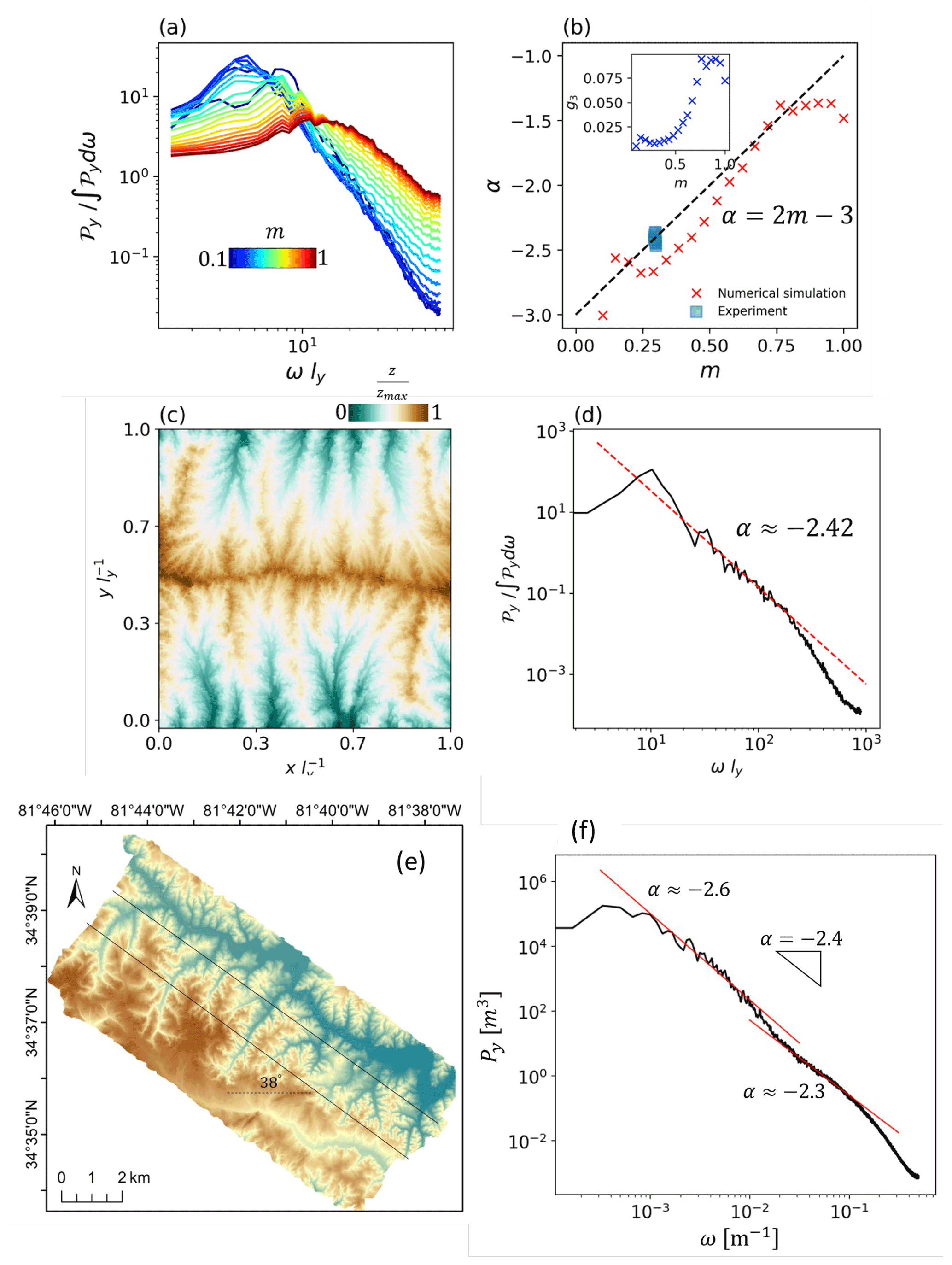
Figure 8 (a) PSDs of elevation longitudinal series for different values of m at an intermediate distance from the boundary. (b) Slope of the power fit to the declining part of the PSD from simulations with 𝒞_I≥10⁵, denoted by α, as a function of the exponent m. The data from the XLE physical experiment are also shown. The black line is the relation $\mathit{\alpha }=\mathrm{2}m-\mathrm{3}$ derived from dimensional and self-similarity arguments in Eq. (43). The inset shows the function g₃(m) from numerical simulations. Panel (c) shows an example of the XLE experimental landscape (Hooshyar et al., 2019), of which panel (d) shows the PSD. (e) Portion of the landscape at the Calhoun Critical Zone Observatory in South Carolina, USA, from 1 m resolution lidar data. (f) The PSD is computed from one-dimensional transects within the area contained by the two parallel lines that are located at an intermediate distance from the main channel showing two distinct power-law scaling regions with similar exponents. After Hooshyar et al. (2021).

From a geomorphological point of view, the connection between the exponent α and the parameter m in the erosion term provides a useful link to landscape processes, since steep landscapes with debris‐flow‐dominated channels have been associated with smaller m, while flatter fluvial landscapes are characterized by larger values of m (Montgomery and Foufoula-Georgiou, 1993). The values of the spectral exponent are also interesting from a more theoretical point of view in relation to the role of nonlinearities as a function of scale. Our analysis has shown consistently values of $\mathit{\alpha }\sim -\mathrm{2.5}$, while several studies previously reported exponents near −2 (Newman and Turcotte, 1990; Huang and Turcotte, 1989; Passalacqua et al., 2006); the latter corresponds to a fractal dimension D_m=1.5 (Huang and Turcotte, 1989; Voss, 1985) and to the presence of an underlying fractional Brownian noise (Turcotte, 1987; Bell, 1975) with a Lorentzian spectrum and an exponential decay of the elevation autocorrelation. These models with $\mathit{\alpha }=-\mathrm{2}$ would therefore imply linear stochastic dynamics at odds with the known presence of nonlinear terms responsible for the very formation of the channel network. On the one hand, $\mathit{\alpha }=-\mathrm{2.5}$ would mean an erosion exponent m=0.25, therefore preserving the nonlinearity of the dynamics also for macroscopic scaling relationships, like the PSD scaling. On the other hand, the fact that the observed value is not far from $\mathit{\alpha }=-\mathrm{2}$ might mean that averages taken over complex landscape patterns cause an effective reduction of nonlinearity, whereby the activation of many degrees of freedom at high channelization regimes causes a statistical regularity which muffles the small-scale nonlinearities. This is certainly an interesting topic that deserves further investigation.

Finally, from a practical point of view, the spectral scaling of landscape elevation could be profitably utilized in developing efficient numerical simulations of landscape evolution (Passalacqua et al., 2006). Such numerical schemes would potentially resemble large eddy simulation methods used in fluid turbulence (Pope, 2000), where the unsolved dynamics at finer scales are approximated by extrapolating the PSD. The improved speed would be a great asset for large-scale simulations of landscape evolution under different scenarios.

4 Conclusions

We have presented several examples of applications of the Π theorem and self-similar scaling to the partitioning of water and sediments driven by the terrestrial water cycle. It is time to draw to a close and ask ourselves whether by using dimensional analysis we have learned anything useful regarding these problems. An answer in the affirmative is suggested by considering that dimensional analysis helped reveal the dominant controls of the dryness index and storage index in the long-term rainfall partitioning, while in the weathering analysis it allowed us to extract the key nonlinear control of the dryness index, making order in the vast amount of information contained in global datasets from different experiments and environmental conditions. Finally, the analysis of the complex geometries obtained from landscape evolution models allowed us to discover new macroscopic relations among macroscopic variables in the partitioning of sediments, the elevation profile, and the spectral scaling. The analogy between landscape elevation and turbulent velocity fluctuations has also been fruitful and promises further results.

If these observations confirm the utility of dimensional analysis, it should also be clear that these methods are not a foolproof set of rules to achieve miraculous solutions. Rather, they are an iterative procedure to sharpen our hypotheses on physical processes. Thinking of dimensional arguments as a form of modeling allows an “explication of the role abstraction and multiple realisability; not as compatibility with other possible worlds but as compatibility with different fictional descriptions of our own world” (Pexton, 2014). The emergence of scaling laws is often only asymptotic (Koutsoyiannis et al., 2018), as in the self-similarity approximations of Sect. 2.2.1, while in several instances it is either difficult to reduce the number of variables in the starting physical law or the problems are hard to formalize in terms of standard dimensions (e.g., in problems interfacing with the social sciences and economics). These challenges notwithstanding, we hope however that these considerations will help breathe new life into Strahler's view (Strahler, 1958) that dimensional analysis will become increasingly useful in hydrology, geomorphology, and beyond.

Appendix A: The Rayleigh–Riabouchinsky controversy: thermodynamic limit as complete self-similarity

In this Appendix we discuss in more detail the Rayleigh–Riabouchinsky controversy related to augmented dimensional analysis. In particular, after a brief historic background, we show how the thermodynamic approach of Rayleigh corresponds to a self-similar solution of the first kind with respect to the dimensionless group obtained from the Boltzmann constant, which serves as the dimensional unifier when augmenting the dimensional analysis from mechanics to thermodynamics.

As mentioned in the main text, Rayleigh (1915a)² considered the problem of the heat flux h, the governed quantity, between a body of characteristic dimension ℓ and a stream of incompressible and inviscid fluid moving with velocity v. Besides ℓ and v, the other governing quantities are the specific heat capacity c and the thermal conductivity κ. Rayleigh formulated a physical law with n=5 governing variables and adopted length, time, energy, and temperature as primary dimensions (i.e., k_Ray=4), as typical in thermodynamics (of course one could also use LMT plus temperature, using mass instead of energy). As a result, he obtained one ($n-k_{\mathrm{Ray}}=\mathrm{5}-\mathrm{4}=\mathrm{1}$) governing dimensionless group, which he used successfully to describe the problem.

In a very short comment published soon after Rayleigh's paper, Riabouchinsky (1915) objected that, adopting the more advanced and detailed point of view of statistical mechanics, according to which temperature is the mean molecular kinetic energy, one could more parsimoniously limit the primary dimensions to length, time, and energy without involving temperature. As a result, he obtained two ($n-k_{\mathrm{Ria}}=\mathrm{5}-\mathrm{3}=\mathrm{2}$) dimensionless groups. In his response, Rayleigh rejected Riabouchinsky's alternative, commenting that

It would indeed be a paradox if the further knowledge of the nature of heat afforded by molecular theory put us in a worse position than before in dealing with a particular problem. The solution would seem to be that the Fourier equations embody something as to the nature of heat and temperature which is ignored in the alternative argument (Rayleigh, 1915b).

Rayleigh's reply was authoritative and sensible but not completely satisfactory. As pointed out by Buckingham (1915): “since he does not pursue the subject further and the reader may feel as if left in mid-air, it seems worth while that the point raised by M. Riabouchinsky should be somewhat further elucidated.” Since then the debate has been the subject of continued discussions. Here, taking a cue from previous analyses of this controversy (e.g., Gibbings, 1980; Butterfield, 2001) and adopting the use of a dimensional unifier (Panton, 2006), we show that Rayleigh's result may be seen as a complete self-similarity solution of the augmented physical law obtained by including the Boltzmann constant as a dimensional unifier to link thermodynamics to mechanics. Starting from a thermodynamic approach to the problem is tantamount to taking for granted the existence of this limit.

Thus, following Rayleigh, we specifically choose length (L), time (T), energy (heat, H), and temperature (Θ) as primary dimensions. With $\left[h\right]=H{T}^{-\mathrm{1}}$, [ℓ]=L, [θ]=Θ, $\left[c\right]=H{L}^{-\mathrm{3}}{\mathrm{\Theta }}^{-\mathrm{1}}$, $\left[\mathit{\kappa }\right]=H{L}^{-\mathrm{1}}{T}^{-\mathrm{1}}{\mathrm{\Theta }}^{-\mathrm{1}}$, $\left[v\right]=L{T}^{-\mathrm{1}}$, and $\left[k_{\mathrm{B}}\right]=H{\mathrm{\Theta }}^{-\mathrm{1}}$, we obtain the dimension matrix

$$\begin{array}{}\text{(A1)}& \begin{array}{lrccrrrr}& h& \mathrm{\ell }& \mathit{\theta }& c& \mathit{\kappa }& v& k_{\mathrm{B}}\\ L& \mathrm{0}& \mathrm{1}& \mathrm{0}& -\mathrm{3}& -\mathrm{1}& \mathrm{1}& \mathrm{0}\\ T& -\mathrm{1}& \mathrm{0}& \mathrm{0}& \mathrm{0}& -\mathrm{1}& -\mathrm{1}& \mathrm{0}\\ H& \mathrm{1}& \mathrm{0}& \mathrm{0}& \mathrm{1}& \mathrm{1}& \mathrm{0}& \mathrm{1}\\ \mathrm{\Theta }& \mathrm{0}& \mathrm{0}& \mathrm{1}& -\mathrm{1}& -\mathrm{1}& \mathrm{0}& -\mathrm{1}\end{array}\end{array}$$

of rank 4. As a result, the Π theorem gives $\mathrm{7}-\mathrm{4}=\mathrm{3}$ dimensionless groups.

Choosing the heat flux h as the governed quantity and selecting ℓ, θ, c, and κ as dimensionally independent (repeating) variables among the governing quantities leads to the physical law

$$\begin{array}{}\text{(A2)}& h=f\left(\mathrm{\ell },\mathit{\theta },c,\mathit{\kappa };v,k_{\mathrm{B}}\right),\end{array}$$

from which the Π theorem then gives

$$\begin{array}{}\text{(A3)}& {\displaystyle \frac{h}{d\mathit{\theta }\mathit{\kappa }}}=\mathit{\phi }\left({\displaystyle \frac{vc\mathrm{\ell }}{\mathit{\kappa }}},{\displaystyle \frac{k_{\mathrm{B}}}{{\mathrm{\ell }}^{\mathrm{3}}c}}\right).\end{array}$$

With a system of units for which k_B=1 and inverting the second Π group, one obtains the result of Riabouchinsky (1915),

$$\begin{array}{}\text{(A4)}& {\displaystyle \frac{h}{\mathrm{\ell }\mathit{\theta }\mathit{\kappa }}}={\mathit{\phi }}_{\mathrm{Ria}}\left({\displaystyle \frac{\mathrm{1}}{{\mathrm{\ell }}^{\mathrm{3}}c}}\right).\end{array}$$

This however would imply the use of very small units, because in the usual SI system, $k_{\mathrm{B}}=\mathrm{1.380649}\times {\mathrm{10}}^{\mathrm{-}\mathrm{23}}$ J K⁻¹. As a result, apart from systems at the nanoscale, in normal conditions $k_{\mathrm{B}}/\left({\mathrm{\ell }}^{\mathrm{3}}c\right)\sim \mathrm{0}$. Our everyday experience, on which thermodynamic concepts are based, shows that we can neglect this term in Eq. (A3) to arrive at the result, originally obtained by Rayleigh,

$$\begin{array}{}\text{(A5)}& {\displaystyle \frac{h}{\mathrm{\ell }\mathit{\theta }\mathit{\kappa }}}={\mathit{\phi }}_{\mathrm{Ray}}\left({\displaystyle \frac{vc\mathrm{\ell }}{\mathit{\kappa }}}\right).\end{array}$$

Thus, looking at Eq. (7), it becomes clear that the thermodynamic limit, which allows us to go from statistical mechanics to continuum mechanics and thermodynamics, corresponds to a complete self-similar solution of Eq. (A3) with respect to $k_{\mathrm{B}}/\left({\mathrm{\ell }}^{\mathrm{3}}c\right)$. It should be stressed that this is not a mathematical fact based solely on the smallness of the Π group, but an empirical ascertainment, as for other self-similar asymptotic regimes (Barenblatt, 1996). Alternatively, the same result is obtained by straightforward application of the Π theorem to the restricted physical law

$$\begin{array}{}\text{(A6)}& h=f_{\mathrm{Ray}}(\mathrm{\ell },\mathit{\theta },c,\mathit{\kappa };v),\end{array}$$

as originally done by Rayleigh.

Appendix B: Derivation of Eq. (28)

We follow here Bonetti et al. (2020) in deriving the equations for the minimalist LEM. The time evolution of the surface elevation $z(x,y,t)$ is described by the sediment continuity equation

$$\begin{array}{}\text{(B1)}& {\displaystyle \frac{\partial z}{\partial t}}=U+\mathrm{\nabla }\cdot \mathbf{f},\end{array}$$

where t is time, U is the uplift rate, and f is the total volumetric sediment flux, given by the sum of fluxes related to runoff erosion (f_c) and soil creep processes (f_d). The latter is assumed to be proportional to the topographic gradient, f_d=δ∇z, δ being a diffusion coefficient. In the so-called detachment-limited conditions all eroded material is considered transported outside the model domain. Thus, with no sediment redeposition, the runoff erosion becomes a sink term, $\mathbf{\nabla }\cdot {\mathbf{f}}_c\approx K_a^{\prime }{q}^m|\mathrm{\nabla }z{|}^n$, where $K_a^{\prime }$ is an erosion coefficient, q is the specific discharge (per unit width of contour line), and m and n are model parameters. As a result, Eq. (B1) becomes

$$\begin{array}{}\text{(B2)}& {\displaystyle \frac{\partial z}{\partial t}}=U-K_a^{\prime }{q}^m|\mathbf{\nabla }z{|}^n+\mathit{\delta }\mathrm{\Delta }z.\end{array}$$

The surface water flux q is linked to the continuity equation

$$\begin{array}{}\text{(B3)}& {\displaystyle \frac{\partial h}{\partial t}}=Q+\mathbf{\nabla }\cdot \left(q\mathbf{n}\right)=Q+\mathbf{\nabla }\cdot \left(hv\mathbf{n}\right),\end{array}$$

where h is the water height, n is the direction of the flow, Q is the part of the rainfall rate that has not infiltrated and that effectively contributes to runoff production, and v is the water velocity. Equation (B3) can be simplified assuming steady-state conditions with constant, representative runoff rate, Q≈Q₀, and speed of water flow v₀ in the direction opposite to the landscape gradient (i.e., $\mathbf{n}=-\mathrm{\nabla }z/\left|\mathrm{\nabla }z\right|$). In such conditions, with the specific discharge being proportional to the water height, q=v₀h, Eq. (B3) becomes

$$\begin{array}{}\text{(B4)}& {\displaystyle \frac{\partial h}{\partial t}}=\mathrm{0}=Q_{\mathrm{0}}+\mathbf{\nabla }\cdot \left(v_{\mathrm{0}}h{\displaystyle \frac{\mathbf{\nabla }z}{\left|\mathbf{\nabla }z\right|}}\right).\end{array}$$

Dividing it by Q₀, Eq. (B4) becomes the equation for the specific catchment area, Eq. (28), with $a=v_{\mathrm{0}}h/Q_{\mathrm{0}}$. Finally, since q=aQ₀, one can write $K_a^{\prime }q=K_a{a}^m$, where $K_a=K_a^{\prime }{Q}_{\mathrm{0}}^m$, thus obtaining Eq. (27).

Appendix C: Analogy with the velocity profile in turbulent flows

Here we report the equation for the streamwise velocity u for the flow between parallel plates to better understand the analogy between the statistics of near-wall turbulence and those of landscape evolution, discussed in Sect. 3.3. We begin with the Navier–Stokes equations for incompressible fluids (Munson et al., 2013),

$$\begin{array}{}\text{(C1)}& \mathit{\rho }{\displaystyle \frac{D\mathbf{v}}{Dt}}=-\mathbf{\nabla }p+\mathit{\mu }\mathrm{\Delta }\mathbf{v}\end{array}$$

and

$$\begin{array}{}\text{(C2)}& \mathrm{\nabla }\cdot \mathbf{v}=\mathrm{0}.\end{array}$$

For the flow between infinite parallel plates, the previous equations give, for the streamwise component u,

$$\begin{array}{}\text{(C3)}& {\displaystyle \frac{\partial u}{\partial t}}={\displaystyle \frac{\partial p}{\partial x}}-u{\displaystyle \frac{\partial u}{\partial x}}-v{\displaystyle \frac{\partial u}{\partial y}}-w{\displaystyle \frac{\partial u}{\partial z}}+\mathit{\mu }\mathrm{\Delta }u.\end{array}$$

Indicating with G the constant pressure gradient and with $\mathbf{q}=\mathit{\{}v,w\mathit{\}}$ the normal velocity

$$\begin{array}{}\text{(C4)}& {\displaystyle \frac{\partial u}{\partial t}}=G-\mathbf{q}\cdot \mathrm{\nabla }u+\mathit{\mu }\mathrm{\Delta }u\end{array}$$

where the Laplacian is only in y and z, the equation becomes similar to the LEM equation (Eq. B2) with $m=n=\mathrm{1}$. Since here the continuity equation is

$$\begin{array}{}\text{(C5)}& {\displaystyle \frac{\partial v}{\partial y}}+{\displaystyle \frac{\partial w}{\partial z}}=\mathrm{0},\end{array}$$

we can write q in terms of a single streamfunction, which automatically satisfies it, i.e.,

$$\begin{array}{}\text{(C6)}& v={\displaystyle \frac{\partial \mathit{\psi }}{\partial z}}\mathrm{and}w=-{\displaystyle \frac{\partial \mathit{\psi }}{\partial y}}.\end{array}$$

We thus have a direct correspondence between the streamwise velocity and the landscape elevation, u↔z, and an indirect one (this is where the equations and the physics obviously differ) between the streamfunction and the specific contributing area ψ↔a. It is also interesting to note that, in these conditions of steady state and x independence, the equations for the other two velocity components and thus also for the streamfunction become decoupled from the equation of u, which means that, unlike the elevation profile, the complex velocity profile in turbulence is shaped by nonstationary terms and streamwise inhomogeneities.