Seasonality of density currents induced by differential cooling

When lakes experience surface cooling, the shallow littoral region cools faster than the deep pelagic waters. The lateral density gradient resulting from this differential cooling can trigger a cold downslope density current that intrudes at the base of the mixed layer during stratified conditions. This process is known as a thermal siphon (TS). TSs flush the littoral region and increase water exchange between nearshore and pelagic zones; thus, they may potentially impact the lake ecosystem. Past observations of TSs in lakes are limited to specific cooling events. Here, we focus on the seasonality of TS-induced lateral transport and investigate how seasonally varying forcing conditions control the occurrence and intensity of TSs. This research interprets 1-year-long TS observations from Rotsee (Switzerland), a small wind-sheltered temperate lake with an elongated shallow region. We demonstrate that TSs occur for more than 50 % of the days from late summer to winter and efficiently flush the littoral region within ∼10 h. We further quantify the occurrence, intensity, and timing of TSs over seasonal timescales. The conditions for TS formation become optimal in autumn when the duration of the cooling phase is longer than the time necessary to initiate a TS. The decrease in surface cooling by 1 order of magnitude from summer to winter reduces the lateral transport by a factor of 2. We interpret this transport seasonality with scaling relationships relating the daily averaged cross-shore velocity, unit-width discharge, and flushing timescale to the surface buoyancy flux, mixed-layer depth, and lake bathymetry. The timing and duration of diurnal flushing by TSs relate to daily heating and cooling phases. The longer cooling phase in autumn increases the flushing duration and delays the time of maximal flushing relative to the summer diurnal cycle. Given their scalability, the results reported here can be used to assess the relevance of TSs in other lakes and reservoirs.

1 Introduction

As lateral boundaries in lakes, littoral regions exchange matter and energy with the surrounding watershed. The littoral region receives both sediment and chemicals from the terrestrial environment, including anthropogenic contaminants (Rao and Schwab, 2007). Particulate matter accumulates in the littoral zone (Cyr, 2017), and this biologically active region can host unique and intensified biogeochemical reactions (Wetzel, 2001). Cross-shore flows, which transport water laterally, connect a lake's littoral region to its pelagic region, thereby facilitating critical ecosystem processes (MacIntyre and Melack, 1995). They control the residence time of nearshore waters and redistribute heat as well as dissolved and particulate compounds throughout the lake. Representing lakes as isolated vertical water columns fails to account for the effects of cross-shore flows on lake biogeochemistry (Effler et al., 2010; Hofmann, 2013).

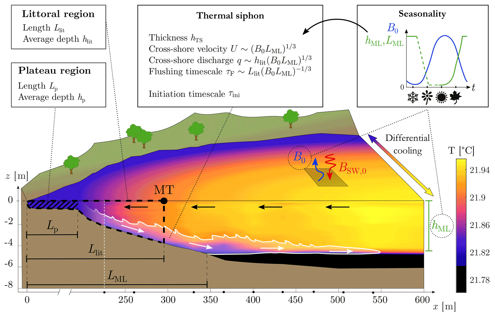
Figure 1 Data-based schematic of the cooling-driven thermal siphon. The schematic shows the plateau, littoral, and mixed regions; the seasonality of the forcing; and the variables used for the transport scaling. Here, the littoral zone is the region upslope of the MT mooring, where the current velocity is measured and transport variables are calculated. The cross-shore temperature field is linearly interpolated from a transect of conductivity–temperature–depth (CTD) profiles collected on the morning of 22 August 2019 (08:20–08:50 UTC), from x=225 m (white dashed line) to x=714 m. Black dots on the x axis show the location of the profiles. The green dashed line in the seasonality diagram corresponds to the transition period between the mixing period (winter) and the stratified period (summer), when the mixed layer is not well defined.

Various mechanisms drive horizontal exchange flows. The pioneer limnologists have already elucidated the effect of large-scale surface and internal gravity waves on horizontal transport (Forel, 1895; Wedderburn, 1907; Mortimer, 1952). In addition to serving as the primary energy source for gravity waves, wind is also responsible for fueling lateral flows via wind-driven cross-shore circulation, cross-shore Ekman transport in rotating environments, and differential deepening (Imberger and Patterson, 1989; Brink, 2016). Buoyancy-driven lateral flows can be induced by horizontal temperature gradients due to differential heating or cooling. Such gradients could form when heat fluxes are spatially heterogeneous, due to large-scale differences in meteorological forcing (Verburg et al., 2011), variable geothermal heating (Roget et al., 1993), shading from vegetation (Lövstedt and Bengtsson, 2008), wind sheltering (Schlatter et al., 1997), or variation in turbidity (MacIntyre et al., 2002). Horizontal temperature gradients also occur when waters with variable depth experience a spatially uniform heat flux (Horsch and Stefan, 1988; Monismith et al., 1990). For a given surface area, the volume of water in the shallow littoral region is less than its offshore counterpart. Thus, littoral waters will cool or warm faster than pelagic waters. Monismith et al. (1990) designated cross-shore circulation resulting from a bathymetrically induced temperature gradient as a thermal siphon. The fact that all lakes have sloping boundaries makes thermal siphons potentially ubiquitous.

This study focuses on thermal siphons driven by differential cooling, wherein the lake temperature exceeds the temperature of maximum density (Fig. 1). The study does not consider heating-driven thermal siphons because induced lateral exchange remains weaker and more sensitive to wind disturbance than cooling-driven thermal siphons (Monismith et al., 1990; James et al., 1994). Atmospheric forcing affects lakes at diurnal, seasonal, or synoptic scales. This includes periods of net cooling when the net surface heat flux is directed towards the atmosphere (Bouffard and Wüest, 2019). This diel or seasonal surface cooling mixes and deepens the surface layer by penetrative convection. Once the shallow littoral region becomes fully mixed, it cools down faster than the deep pelagic region. Littoral waters become denser and plunge as a downslope density current, which intrudes at the base of the mixed layer during stratified conditions. At the surface, a reverse flow brings water from the pelagic to the littoral region (Horsch and Stefan, 1988; Monismith et al., 1990). We will hereafter refer to the density current induced by differential cooling simply as a thermal siphon (TS).

TSs have often been evoked to explain cold anomalies observed in lakes; these include tilted isotherms above the sloping sides (Talling, 1963; Eccles, 1974; MacIntyre and Melack, 1995; Woodward et al., 2017) or cold water intrusions (Wells and Sherman, 2001; Peeters et al., 2003; Rueda et al., 2007; Forrest et al., 2008; Ambrosetti et al., 2010). However, only a few studies have provided detailed in situ descriptions of the process. The first extensive studies of TSs assessed power plant heat disposal within cooling lakes (Adams and Wells, 1984). Warm water discharged into these reservoirs flows onshore at the surface, cools, and induces a TS in sidearms. However, these observations are not representative of naturally formed TSs. Cooling lakes constantly receive heat from power plants, which increases the intensity and duration of surface cooling compared with that experienced in other lakes and reservoirs (Horsch and Stefan, 1988). An extensive review of the literature suggests that Monismith et al. (1990) provided the first in situ observations of a diurnal cycle associated with a naturally formed TS. The authors studied a sidearm of Wellington Reservoir (Australia) in summer and described the complete diurnal cycle of daytime differential heating and nighttime differential cooling. In both cases, they observed cross-shore flows at velocities of ∼2 cm s⁻¹. Cross-shore circulation was characterized by inertia with a delay of several hours between the shift in forcing conditions and the flow reversal. Other studies have reported the presence of TSs along the thalweg of narrow reservoir embayments (James and Barko, 1991a, b; James et al., 1994; Rogowski et al., 2019) but also along the sloping sides of lakes (Sturman et al., 1999; Thorpe et al., 1999; Fer et al., 2002a, b; Pálmarsson and Schladow, 2008) and between different basins (Roget et al., 1993). In most of these examples, TS characteristics comported with the description given in Monismith et al. (1990). These included thermal stratification above the sloping bottom, inertial effects, and a cross-shore velocity on the order of 1 cm s⁻¹. The work by Fer et al. (2002b) on the sloping sides of Lake Geneva (Switzerland) represents one of the most extensive TS studies. The authors collected continuous measurements over two winters and identified density currents initiated in the middle of the night and lasting until the late morning. The research detected increasing discharge with distance downslope and found that one TS event could flush the littoral region almost twice.

The lake stratification and the intensity and duration of the daily cooling period vary seasonally (Bouffard and Wüest, 2019). These changes in forcing conditions may affect the occurrence and magnitude of TSs over time. Previous studies have focused on specific TS events and did not monitor the process over different seasons. A 3-year-long dataset on Lake Anna (VA, USA; Adams and Wells, 1984) addressed a cooling lake and, thus, did not reflect the seasonality of naturally formed TSs. Although the time series collected by Roget et al. (1993) between two lobes of Lake Banyoles (Spain) spans 8 months (October–May), these authors do not address seasonal variability in the observed TS. Geothermal fluxes between the lobes enhance differential cooling in Lake Banyoles, which may modify TS seasonality. James and Barko (1991b) performed six tracer experiments between June and September. These authors obtained estimates of TS velocity that varied between the experiments and were higher for days with stronger lateral temperature gradients. While the experiments did not identify a clear seasonal trend, thermistor arrays detected an increase in the occurrence of differential cooling from May to August, suggesting a higher frequency of TS events in late summer. This hypothesis was not verified due to the lack of long-term velocity measurements. Thus, the seasonality of TS occurrence and intensity has not been systematically investigated in lakes.

Dimensional analysis and laboratory experiments have provided relationships linking forcing and background conditions (surface cooling, stratification) to cross-shore transport by TSs (Harashima and Watanabe, 1986), but these lack validation in the field. The comprehension of the TS seasonality would improve the prediction of TS events in lakes and their contribution to exchanges between littoral and pelagic regions. The present research monitored TSs in a small temperate lake over a 1-year period. The study establishes three characteristics of TS seasonality including its occurrence (Sect. 3.3), intensity (Sect. 3.4), and diurnal dynamics (Sect. 3.5). The observed TS seasonality clearly relates to forcing parameters and, thus, pinpoints key parameters for predicting TS events in lakes (Sect. 4). The observation and interpretation of TS events across seasonal timescales provides a comprehensive understanding of the conditions required to form TSs in lakes.

2 Methods

2.1 Study site and field measurements

Rotsee is a small peri-alpine monomictic lake near Lucerne, Switzerland (Fig. 2a). It is located at 419 m a.s.l. (above sea level) and has a surface area of 0.5 km² with a mean and maximum depth of 9 and 16 m, respectively. The main in- and outflows are located at the southwestern and northeastern ends of the lake, respectively, and have a low discharge of ∼0.1 m³ s⁻¹. Rotsee is an elongated lake (2.5 km long, 0.2 km wide), with steep sides (slope of 15^∘) across its longitudinal axis and more gradual slopes (1.5^∘) at its two ends. The northeastern end of the lake finishes with a 200 m long plateau region of approximately 1 m depth that can trigger TSs. Moreover, Rotsee is located in a depression and sheltered from wind; hence, it is famous for international rowing championships and an ideal field-scale laboratory where convective processes are distinctively observable.

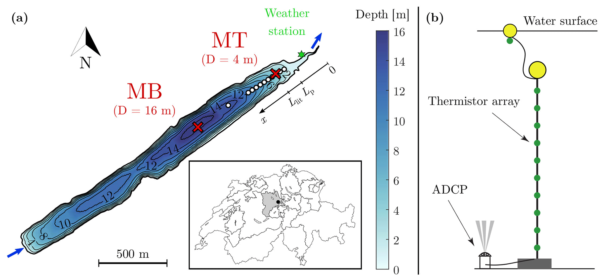
Figure 2 (a) Bathymetry of Rotsee indicating the location of the two moorings MB and MT (red crosses), the cross-shore transect of CTD profiles (white dots), the weather station (green star), and the length of the plateau and littoral regions (L_p and L_lit, respectively). Blue arrows correspond to the main inflow and outflow. The location of Rotsee is shown on the map of Switzerland using a black dot (source: Federal Office of Topography). (b) Schematic of the mooring MT. A similar setup is used for the thermistor array at MB. The detailed setup is provided in Appendix A.

This study focuses on quantifying TSs originating from the northeastern plateau region (Fig. 2a). Because of the elongated shape of Rotsee, we use the 2D (x, z) framework shown in Fig. 1 by orienting the x axis along the thalweg. We assume that TSs flow preferentially along the x axis, and we neglect the influence of perpendicular flows. We will now refer to the northeastern end of the lake as the “shore” and call the direction of the x axis the “offshore direction”.

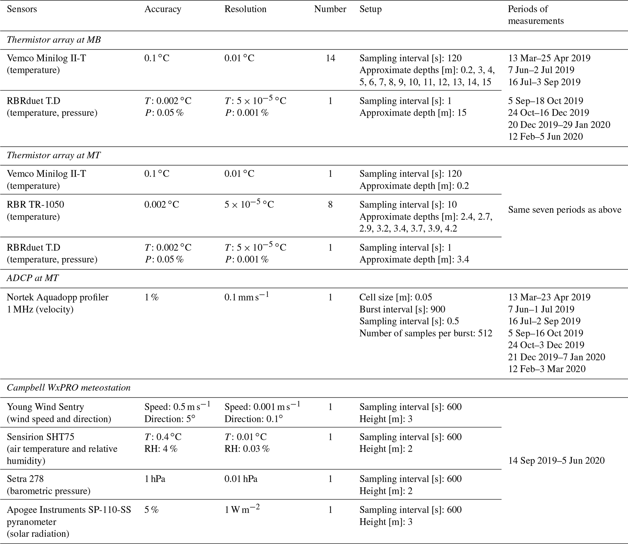
We monitored the background stratification at the deepest location (“background mooring” MB, approx. 16 m deep) as well as the dynamics of TSs off the plateau region (“TS mooring” MT, approx. 4 m deep) from March 2019 to March 2020 (Fig. 2a). Mooring MT was located along the thalweg, at the beginning of the sloping region. This shallow water column is already vertically mixed in summer by the action of surface cooling. We briefly describe the moorings below and provide more detailed information on the specifications and setup of the instruments in Appendix A. Each mooring included an array of thermistors (Fig. 2b). The evolution of the background temperature was monitored at MB with Vemco Minilog II-T loggers (accuracy: 0.1 ^∘C). High-resolution thermistors RBR TR-1050 and RBRduet T.D (accuracy: 0.002 ^∘C) were used at MT to track finer-scale temperature fluctuations near the sloping boundaries. The thermistors were installed from 1 to 13 m above the bottom with a 1 m vertical resolution at MB and from 0.25 to 2 m above the bottom with a 0.25 m resolution at MT. The evolution of the near-surface temperature (0.2 to 0.3 m below the surface) was monitored with Vemco loggers attached to surface buoys at both locations. An upward-looking acoustic Doppler current profiler (ADCP, Nortek Aquadopp profiler 1 MHz) was deployed at MT for fine-scale measurements of the bottom currents (Fig. 2b). It collected velocity profiles with a vertical bin resolution of 0.05 m from 0.25 to 3 m above the bottom. Velocity was obtained by averaging 512 burst measurements every 15 min. A week-long maintenance of the moorings was conducted every 40 d on average. The measurement periods of the ADCP were shorter in December and January due to low battery (Appendix A). The monitoring was stopped in May 2019 to avoid any hazard during the European Rowing Championships.

A WxPRO Campbell weather station was installed at the lake shore, near the plateau region, in September 2019 (Fig. 2a). It measured atmospheric pressure, air temperature, wind speed, incoming shortwave radiation, and relative humidity every 10 min. In addition, incoming longwave radiation was obtained from the Lucerne weather station (47^∘02^′12^′′ N, 8^∘18^′04^′′ E; source MeteoSwiss), ∼4 km from Rotsee. The Lucerne station also provided meteorological forcing when the reference Rotsee weather station was not measuring (data gaps and period before September 2019). In these cases, the Lucerne dataset was adjusted based on the Rotsee observations from September 2019 to June 2020. Pressure, air temperature, and shortwave radiation were linearly corrected (R²>0.9). This simple method did not allow reliable correction to the relative humidity and wind speed. Instead, we applied a neural network fitting approach to correct these two variables. The shallow neural network consisted of one hidden layer with 50 neurons and was trained by a Levenberg–Marquardt algorithm. A total of 70 % of the reference period from September 2019 to June 2020 was used to train the neural network, and the remaining percentage was equally distributed for validation and testing. All of the meteorological variables measured in Lucerne were used as inputs to the network, and the procedure was repeated for each of the two target variables. The network performance was satisfactory, with a coefficient of determination R² and a root-mean-square error E_RMS between observations and estimates of R²≈0.72 and E_RMS≈0.67 m s⁻¹ for wind speed and of R²≈0.94 and E_RMS≈4.7 % for relative humidity. The uncertainty in wind speed and relative humidity estimates leads to an average uncertainty of 5 % and 3 % of the surface heat fluxes (Sect. 2.2), respectively.

We captured the spatial variability in TSs on the morning of 22 August 2019 (Fig. 1) by collecting 11 conductivity–temperature–depth (CTD) profiles (CTD60M, Sea & Sun Technology) along the x axis, between 2 and 14 m depth (Fig. 2a).

2.2 Heat and buoyancy fluxes

Heat fluxes were estimated from meteorological data and lake surface temperature at MB. We assumed that the meteorological conditions and the heat fluxes were spatially uniform over the lake surface (0.5 km²). Heat fluxes were defined positive in the upward direction (lake cooling) and negative in the downward direction (lake heating). The non-penetrative surface heat flux $H_{Q_{\mathrm{0}}}$ is defined as

$$\begin{array}{}\text{(1)}& H_{Q_{\mathrm{0}}}=H_C+H_E+H_{\mathrm{LW},\mathrm{in}}+H_{\mathrm{LW},\mathrm{out}}\left[\mathrm{W}{\mathrm{m}}^{-\mathrm{2}}\right],\end{array}$$

where H_C and H_E are the respective sensible and latent heat fluxes, and H_LW,in and H_LW,out are the respective incoming and outgoing longwave radiation. The net surface heat flux H_0,net includes the shortwave radiative flux at the surface H_SW,0:

$$\begin{array}{}\text{(2)}& H_{\mathrm{0},\mathrm{net}}=H_{Q_{\mathrm{0}}}+H_{\mathrm{SW},\mathrm{0}}\left[\mathrm{W}{\mathrm{m}}^{-\mathrm{2}}\right].\end{array}$$

The different terms of the heat budget were calculated similarly to Fink et al. (2014). Cloudiness modulates the proportion of direct and diffuse shortwave radiation and was derived from daily clear-sky irradiance as in Meyers and Dale (1983). We modified the empirical wind and air temperature-based calibration function, f, in the sensible and latent heat flux estimates of Fink et al. (2014) to take the lake fetch into account, as proposed in McJannet et al. (2012).

The non-penetrative surface buoyancy flux B₀ was inferred from $H_{Q_{\mathrm{0}}}$ under the assumption that only heat fluxes modify the potential energy near the surface (Bouffard and Wüest, 2019):

$$\begin{array}{}\text{(3)}& B_{\mathrm{0}}={\displaystyle \frac{\mathit{\alpha }g{H}_{Q_{\mathrm{0}}}}{\mathit{\rho }{C}_{\mathrm{p},\mathrm{w}}}}\left[\mathrm{W}{\mathrm{kg}}^{-\mathrm{1}}\right].\end{array}$$

In Eq. (3), $\mathit{\alpha }=-(\mathrm{1}/\mathit{\rho })\partial \mathit{\rho }/\partial T$ is the thermal expansivity of water [^∘C⁻¹], g is the gravitational acceleration [m s⁻²], ρ is the water density [kg m⁻³], and C_p,w is the specific heat of water [J ^∘C⁻¹ kg⁻¹]. The thermal expansivity was estimated from the surface temperature using the relationship reported in Bouffard and Wüest (2019). To calculate water density, we used the equation of state from Chen and Millero (1986), with a measured average salinity of S=0.2 g kg⁻¹ for Rotsee. Our analysis assumed a constant salinity over the year, as the seasonal changes in surface density are controlled by temperature fluctuations rather than variations in salinity.

Similarly, a radiative surface buoyancy flux B_SW,0 was obtained as follows:

$$\begin{array}{}\text{(4)}& B_{\mathrm{SW},\mathrm{0}}={\displaystyle \frac{\mathit{\alpha }g{H}_{\mathrm{SW},\mathrm{0}}}{\mathit{\rho }{C}_{\mathrm{p},\mathrm{w}}}}\left[\mathrm{W}{\mathrm{kg}}^{-\mathrm{1}}\right].\end{array}$$

The net buoyancy flux at the surface is $B_{\mathrm{0},\mathrm{net}}=B_{\mathrm{0}}+B_{\mathrm{SW},\mathrm{0}}$. $B_{\mathrm{0},\mathrm{net}}>\mathrm{0}$ indicates a destabilizing buoyancy flux (net cooling), whereas $B_{\mathrm{0},\mathrm{net}}<\mathrm{0}$ indicates a stabilizing buoyancy flux (net heating). We used B_0,net to identify the daily cooling and heating phases (Sect. 3.1), and we averaged B₀ over the daily cooling phase to quantify the intensity of convection (Sect. 2.6).

2.3 Mixed-layer depth

We used hourly averaged temperature data from MB to calculate the thermocline depth (h_t) and the mixed-layer depth (h_ML). Based on the review of Gray et al. (2020), we estimated h_ML using the temperature-gradient method with a threshold of $\mathrm{d}T/\mathrm{d}z=\mathrm{0.05}$ ^∘C m⁻¹. The water column was defined as fully mixed when $\mathrm{d}T/\mathrm{d}z<\mathrm{0.05}$ ^∘C m⁻¹ at all depths. In this case, h_ML was set to the depth of the bottom temperature sensor. For stratified conditions, the thermocline depth was defined as the depth of maximum gradient in $\mathrm{d}T/\mathrm{d}z$. Starting from h_t and moving upward, the lower end of the mixed layer was reached when the local temperature gradient dropped to $\mathrm{d}T/\mathrm{d}z<\mathrm{0.05}$ ^∘C m⁻¹. When $\mathrm{d}T/\mathrm{d}z>\mathrm{0.05}$ ^∘C m⁻¹ at all depths, the entire column was stratified and h_ML was zero.

2.4 Occurrence of thermal siphons

We used the velocity data from the Aquadopp profiler at MT to estimate the cross-shore transport over the bottom 3 m of the sloping region. Quality control of the velocity was performed by discarding values with beam correlation below 50 % or signal amplitude weaker than 6 dB above noise floor. The horizontal velocity was projected onto the x axis (angle of 56^∘ from north), which crosses the isobath at MT perpendicularly (Fig. 2a). Following the 2D framework of Fig. 1, we will now call U_x the “cross-shore velocity”.

The time series of U_x was then divided into 24 h subsets, starting and ending at 17:00 UTC. Each 24 h subset was analyzed separately to identify TS events. We decided to focus on periods when MT was located in the sloping mixed region, with TSs flowing at the bottom of the water column (Fig. 1). This condition allowed us to relate our current measurements to scaling formulae of downslope density currents (Sect. 3.4). A downslope TS event was detected on a specific day if the three following conditions were met:

1. There was significant cross-shore flow, where the depth-averaged velocity of the current $\stackrel{\mathrm{‾}}{U_x}>\mathrm{0.5}$ cm s⁻¹ for at least 2 h;

2. There was weak wind during the selected event, where $\mathrm{|}{L}_{\mathrm{MO},\mathrm{avg}}\mathrm{|}/h_{\mathrm{ML},\mathrm{avg}}<\mathrm{0.5}$ (L_MO,avg and h_ML,avg are the averaged Monin–Obukhov length scale (Wüest and Lorke, 2003) and mixed-layer depth during the cross-shore flow event, respectively);

3. There was a mixed water column at MT before the onset of the flow, where $\mathrm{d}T/\mathrm{d}z<\mathrm{0.05}$ ^∘C m⁻¹ at all depths.

Cross-shore flows that did not meet conditions no. 2 and no. 3 were noted as “wind-driven circulation” and “stratified flows”, respectively. The term “stratified flows” refers here to any cross-shore flow that occurred when the mixed-layer depth was shallower than the lake depth at MT. This includes basin-scale internal waves and intruding TSs. Further justifications of the above criteria are provided in Appendix D.

2.5 Cross-shore transport by thermal siphons

The cross-shore transport was calculated for each identified TS event (Sect. 2.4). For each event, we defined subperiods with continuous positive U_x (further details in Appendix D). We calculated the unit-width volume of water transported over each of these subperiods:

$$\begin{array}{}\text{(5)}& V_{x,i}=\underset{t_{\mathrm{0},i}}{\overset{t_{\mathrm{f},i}}{\int }}{q}_x\left(t\right)\mathrm{d}t\left[{\mathrm{m}}^{\mathrm{2}}\right],\end{array}$$

where t_0,i and t_f,i are the initial and final times of subperiod i, respectively, and q_x is the unit-width discharge defined as

$$\begin{array}{}\text{(6)}& q_x\left(t\right)=\underset{z_{\mathrm{bot}}\left(t\right)}{\overset{z_{\mathrm{top}}\left(t\right)}{\int }}{U}_x(z,t)\mathrm{d}z\left[{\mathrm{m}}^{\mathrm{2}}{\mathrm{s}}^{-\mathrm{1}}\right].\end{array}$$

In Eq. (6), z_bot and z_top are the respective bottom and top interfaces of the region over which U_x>0 at time t. For each day, we then defined the TS flushing period as the subperiod with the largest volume transported V_x,i.

Four daily quantities characterizing the cross-shore transport were calculated over the flushing period of each day ($t_{\mathrm{0}}\le t\le t_{\mathrm{f}}$): the average cross-shore velocity U_avg and unit-width discharge q_avg, the maximum cross-shore velocity U_max (both in time and depth), and the flushing timescale ${\mathit{\tau }}_{\mathrm{F}}=V_{\mathrm{lit}}/q_{\mathrm{avg}}$, with V_lit≈500 m² representing the unit-width volume of the littoral region upslope of MT (Fig. 1). U_avg and q_avg were obtained as follows:

$$\begin{array}{}\text{(7)}& {\displaystyle }& {\displaystyle }{U}_{\mathrm{avg}}={\displaystyle \frac{\mathrm{1}}{t_{\mathrm{f}}-t_{\mathrm{0}}}}\underset{t_{\mathrm{0}}}{\overset{t_{\mathrm{f}}}{\int }}\stackrel{\mathrm{‾}}{U_x\left(t\right)}\mathrm{d}t\left[\mathrm{m}{\mathrm{s}}^{-\mathrm{1}}\right],\text{(8)}& {\displaystyle }& {\displaystyle }{q}_{\mathrm{avg}}={\displaystyle \frac{\mathrm{1}}{t_{\mathrm{f}}-t_{\mathrm{0}}}}\underset{t_{\mathrm{0}}}{\overset{t_{\mathrm{f}}}{\int }}{q}_x\left(t\right)\mathrm{d}t\left[{\mathrm{m}}^{\mathrm{2}}{\mathrm{s}}^{-\mathrm{1}}\right].\end{array}$$

2.6 Scaling formulae

We relate the transport quantities introduced in Sect. 2.5 to the forcing parameters using scaling formulae from theoretical and laboratory studies.

The horizontal velocity scale of TSs is $U\sim (B_{\mathrm{0}}L{)}^{\mathrm{1}/\mathrm{3}}$, where B₀ is the destabilizing surface buoyancy flux, and L is a horizontal length scale (Phillips, 1966). Following Wells and Sherman (2001), we used the horizontal length scale L_ML based on the mixed-layer depth:

$$\begin{array}{}\text{(9)}& U=c_U{\left(B_{\mathrm{0}}{L}_{\mathrm{ML}}\right)}^{\mathrm{1}/\mathrm{3}}\left[\mathrm{m}{\mathrm{s}}^{-\mathrm{1}}\right],\end{array}$$

where c_U is a proportionality coefficient. For each value of h_ML, we calculated L_ML as the distance between the northeastern edge of the lake and the location where the mixed layer intersects the lake sloping bottom (Fig. 1).

The unit-width discharge is scaled by $q\sim (B_{\mathrm{0}}L{)}^{\mathrm{1}/\mathrm{3}}h$, where h is a vertical length scale. We used the average depth of the littoral region upslope of MT ($h_{\mathrm{lit}}=V_{\mathrm{lit}}/L_{\mathrm{lit}}$, Fig. 1) as h:

$$\begin{array}{}\text{(10)}& q=c_q{\left(B_{\mathrm{0}}{L}_{\mathrm{ML}}\right)}^{\mathrm{1}/\mathrm{3}}{h}_{\mathrm{lit}}\left[{\mathrm{m}}^{\mathrm{2}}{\mathrm{s}}^{-\mathrm{1}}\right],\end{array}$$

where c_q is a proportionality coefficient. We defined the flushing timescale from Eq. (10) as

$$\begin{array}{}\text{(11)}& {\mathit{\tau }}_{\mathrm{F}}={\displaystyle \frac{V_{\mathrm{lit}}}{q}}=c_{\mathrm{F}}{\displaystyle \frac{L_{\mathrm{lit}}}{{\left(B_{\mathrm{0}}{L}_{\mathrm{ML}}\right)}^{\mathrm{1}/\mathrm{3}}}}\left[\mathrm{s}\right],\end{array}$$

where $c_{\mathrm{F}}=\mathrm{1}/c_q$. The flushing timescale represents the time that a TS needs to flush the littoral region of volume V_lit.

The daily cooling phase of duration τ_c is defined by $B_{\mathrm{0},\mathrm{net}}>\mathrm{0}$. After the onset of surface cooling, a TS does not form immediately. Vertical convective mixing takes place before the horizontal density gradient starts to drive a TS (Wells and Sherman, 2001; Ulloa et al., 2022). The period between the start of the cooling phase and the TS formation is quantified by an initiation timescale (τ_ini). If the littoral region is initially mixed vertically, τ_ini equals the transition timescale τ_t derived by Ulloa et al. (2022) under constant surface cooling:

$$\begin{array}{}\text{(12)}& {\mathit{\tau }}_{\mathrm{t}}={\displaystyle \frac{\mathrm{2}{\left(L_{\mathrm{ML}}-L_{\mathrm{p}}\right)}^{\mathrm{2}/\mathrm{3}}}{B_{\mathrm{0}}^{\mathrm{1}/\mathrm{3}}{\left(\mathrm{1}-h_{\mathrm{p}}/h_{\mathrm{ML}}\right)}^{\mathrm{1}/\mathrm{3}}}}\left[\mathrm{s}\right],\end{array}$$

where L_p≈170 m and h_p≈1 m, representing the length and depth of the plateau region of Rotsee, respectively (Fig. 1). This timescale is based on a three-way momentum balance between the lateral pressure gradient due to differential cooling and the inertial terms (Finnigan and Ivey, 1999).

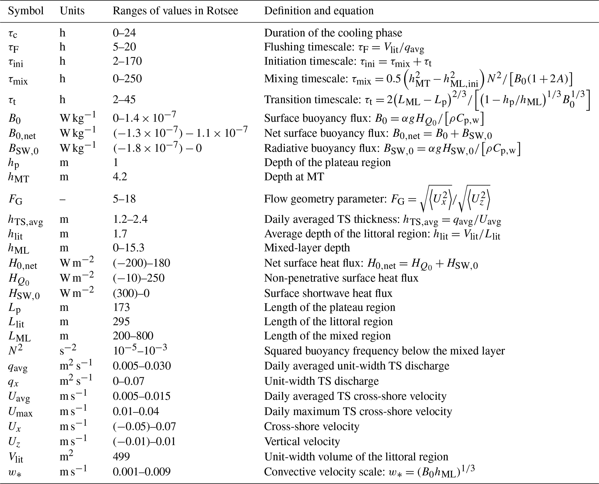
In Eqs. (9)-(12), B₀ and L_ML are averaged over τ_c every day. We discuss the choice of the length scales L_ML and h_lit in more detail in Sect. 4.3. The key parameters used for the scaling formulae and TS dynamics are listed in Table 1.

Table 1 Key parameters related to the forcing parameters, bathymetry, and TS dynamics. For seasonally varying parameters, the given ranges of values are daily averages.

3 Results

3.1 Diurnal cycle

The magnitude of the net surface buoyancy flux B_0,net oscillates daily, and the intensity of the diel fluctuation is modulated at a seasonal timescale (Fig. 3a). We illustrate the diurnal cycle with an example on 9–10 September 2019 (Fig. 3b, c, d). This summertime period is characterized by a strong day–night variability, which is ideal to elucidate how changes in forcing conditions affect the formation and destruction of TSs. The net surface buoyancy flux B_0,net varies from $-\mathrm{2}\times {\mathrm{10}}^{-\mathrm{7}}$ W kg⁻¹ during daytime to $\mathrm{1}\times {\mathrm{10}}^{-\mathrm{7}}$ W kg⁻¹ during nighttime (Fig. 3b). In contrast to B_0,net, B₀ remains positive over 24 h, indicating a continuous cooling at the air–water interface. In late summer, B₀ is $\sim {\mathrm{10}}^{-\mathrm{7}}$ W kg⁻¹ with a limited variability of $\pm \mathrm{5}\times {\mathrm{10}}^{-\mathrm{8}}$ W kg⁻¹ between day and night. The radiative forcing B_SW,0 is the main driver of the diurnal variability, with diel variations that are 1 order of magnitude larger than B₀ during cloud-free summer days like 9–10 September 2019. We observe differential cooling at night, with lateral temperature gradients of $\sim \mathrm{5}\times {\mathrm{10}}^{-\mathrm{4}}$ ^∘C m⁻¹ in late summer (Fig. 1).

Figure 3 Diurnal cycle of a TS. (a) Net surface buoyancy flux as a function of time during the day, represented over 1 year (from 13 March 2019 to 13 March 2020). DOY stands for “day of the year”. A 30 d moving average has been applied to smooth the time series. The 45 d long period without measurement in May 2019 is shown in gray. The contour lines have a spacing of $\mathrm{1}\times {\mathrm{10}}^{-\mathrm{7}}$ W kg⁻¹. The dashed line corresponds to the diurnal cycle shown in panels (b), (c), and (d) (9–10 September 2019; DOY 252–253). (b) Time series of surface buoyancy fluxes defining the cooling and heating phases on 9–10 September 2019. (c) Vertical velocity measured every 15 min at MT (depth of ∼4 m) as a function of time and height above the sediment. Positive (purple) values correspond to a flow moving upward. Strong vertical movements are the signature of convective plumes. (d) Cross-shore velocity measured every 15 min at MT as a function of time and height above the sediment. Positive (purple) values correspond to a flow moving offshore (southwestward flow). Black lines are 0.05 ^∘C spaced isotherms that are linearly interpolated between each thermistor. The TS detected by the algorithm and used for the transport calculation is depicted in blue. The vertical resolution of the thermistors is shown by the horizontal black ticks on the right axis. Horizontal arrows identify three periods: (1) deepening of the mixed layer, (2) transition period before the initiation of the TS, and (3) flushing period.

We divide the diurnal cycle into a net cooling phase during the night ($B_{\mathrm{0}}>\mathrm{|}{B}_{\mathrm{SW},\mathrm{0}}\mathrm{|}$) and a net heating phase during the day ($B_{\mathrm{0}}<\mathrm{|}{B}_{\mathrm{SW},\mathrm{0}}\mathrm{|}$). Starting the period at 17:00 UTC, the water column is initially thermally stratified by the radiative heating of the daytime period (Fig. 3d). During the first part of the night, convective cooling mixes and deepens the surface layer (period no. 1 in Fig. 3d). The water column becomes entirely mixed at MT around 00:00 UTC (see the vertical isotherms starting around 00:00 UTC in Fig. 3d). The convective plumes intensify in the second part of the night to reach vertical velocities of ∼5 mm s⁻¹ (Fig. 3c). A total of 3 h after complete vertical mixing at MT, a cross-shore circulation is initiated (period no. 3 in Fig. 3d), with a downslope flow near the bottom (positive U_x) and an opposite flow above (negative U_x). The velocity magnitude of ∼1 cm s⁻¹ is typical for TSs. We will hereafter refer to the period during which a TS flows as the flushing period. The interface between the two flows oscillates vertically by 1–2 m (∼100 % of the TS thickness), suggesting that the transport is limited by the vertical mixing of convective plumes. At the end of the cooling phase, the water column is distinctly stratified near the bottom, indicating the presence of persistent colder water flowing downslope. A striking observation is the intensification of the TS in phase with the weakening of vertical convection at the onset of radiative heating. The cross-shore velocity increases above 2 cm s⁻¹, and the induced bottom stratification reaches ∼0.1 ^∘C m⁻¹ at the beginning of the heating phase. This strong flushing lasts for several hours, while radiative heating increases and re-stratifies the water above the density current. The cross-shore flow weakens in the late morning but continues until noon.

The example detailed above presents all of the characteristics of a typical TS, with different phases and inertia between the cooling phase and the flushing period. Other examples, provided in Appendix B (Fig. B2), show that the timing and magnitude of the flow change with the forcing conditions.

3.2 Seasonal variability in the forcing parameters

Two key parameters for TS formation are B₀ and h_ML (Sect. 2.6), which are indirectly related to B_0,net. Hereafter, we refer to these parameters as “forcing parameters” of TSs. The daily intensity of convective cooling is estimated based on the convective velocity scale $w_{*}=(B_{\mathrm{0}}{h}_{\mathrm{ML}}{)}^{\mathrm{1}/\mathrm{3}}$ (Deardorff, 1970), where B₀ and h_ML are daily averages during the cooling phase at MB. These two parameters are both seasonally dependent, and their relationship is characterized by an annual hysteresis cycle (Fig. 4a). Although the surface heat flux $H_{Q_{\mathrm{0}}}$ increases from winter to summer, the strong seasonal variability in B₀ (1 order of magnitude larger in summer than in winter) is mostly due to seasonal changes in the thermal expansivity α.

Figure 4 Seasonal variability in the forcing parameters over 1 year (from March 2019 to March 2020). (a) Daily averages of mixed-layer depth as a function of surface buoyancy flux during cooling periods. Gray dashed lines indicate the corresponding convective velocity scale. The black dashed line with arrows is a qualitative representation of the annual cycle. (b) Monthly averages of convective velocity scale w_* during the cooling phase (green line), duration of the cooling phase τ_c (blue line), and net surface buoyancy flux B_0,net (linearly interpolated color map). Error bars represent the standard deviation of w_* and τ_c.

From spring to summer, h_ML remains shallow (<2 m) and B₀ increases from $\sim {\mathrm{10}}^{-\mathrm{9}}$ W kg⁻¹ in March to $\sim {\mathrm{10}}^{-\mathrm{7}}$ W kg⁻¹ in August. The latter results in an increase in the convective velocity scale from $w_{*}\approx \mathrm{3.8}\pm \mathrm{0.7}$ to $w_{*}\approx \mathrm{6.7}\pm \mathrm{0.9}$ mm s⁻¹ over the same period (Fig. 4a, b). The lake undergoes net daily heating over this period ($B_{\mathrm{0},\mathrm{net}}<\mathrm{0}$), with a cooling phase that remains shorter than 15 h (Fig. 4b). In August, $B_{\mathrm{0},\mathrm{net}}\approx \mathrm{0}$ and daily heating is balanced by daily cooling. At this period, the intensity of convective mixing reaches its maximum, and the diurnal heating–cooling cycle is pronounced (Fig. 3a).

From September to January, the lake undergoes a daily net cooling ($B_{\mathrm{0},\mathrm{net}}>\mathrm{0})$ and the mixed layer deepens by convection at an average rate of ∼0.1 m d⁻¹, leading to a complete mixing in mid-December. Over the same period, B₀ continuously decreases due to the drop in α with colder temperatures. This decrease in B₀ balances the deepening of h_ML, and w_* remains constant around $w_{*}\approx \mathrm{7}\pm \mathrm{1}$ mm s⁻¹ from August to November. The duration of the cooling phase increases in autumn to reach its maximum in November (${\mathit{\tau }}_{\mathrm{c}}\approx \mathrm{21}\pm \mathrm{2}$ h). Convective cooling is occurring almost continuously at that time. In winter, the convective velocity w_* drops to $w_{*}\approx \mathrm{3.5}\pm \mathrm{1}$ mm s⁻¹, and the effect of the cooling phase is again balanced by the heating phase ($B_{\mathrm{0},\mathrm{net}}\approx \mathrm{0}$, ${\mathit{\tau }}_{\mathrm{c}}\approx \mathrm{15}\pm \mathrm{3}$ h in February). The differences between the cooling and heating phases of the diurnal cycle are reduced in winter, with $B_{\mathrm{0},\mathrm{net}}\approx \mathrm{0}$ over the entire day (Fig. 3a). Note that winter 2019–2020 was warm, and Rotsee remained mixed from December to February (no inverse stratification, surface temperature T>4 ^∘C).

3.3 Seasonal occurrence of thermal siphons

We apply our detection algorithm for cross-shore flows (Sect. 2.4) on 227 d with continuous measurements at MT from March 2019 to February 2020. We identify 156 d with a significant cross-shore flow (69 % of the days with observations), over which 85 d (37 %) were reported as TS events. The remaining days with identified cross-shore flow were either associated with wind-driven circulation for 13 d (6 %) or stratified flows for 58 d (26 %). We estimate the percentage of occurrence of TSs relative to the number of days with measurements (p_TS) for each month (Fig. 5). Before late July, the mixed layer is usually shallower than 4 m (Fig. 4a) and stratified flows prevail at MT (Fig. 5). The first events identified as TSs occur on 28 July and 31 July (p_TS=12.5 % in July). However, TSs do not reach a significant percentage of occurrence (∼50 %) until August. The occurrence increases in autumn to reach 87 % in November. In winter, TSs are less common: they only occur on 38 % of the days in December, 2 d in early January (not shown in Fig. 5 due to the few days measured during this month), and are not observed later in winter.

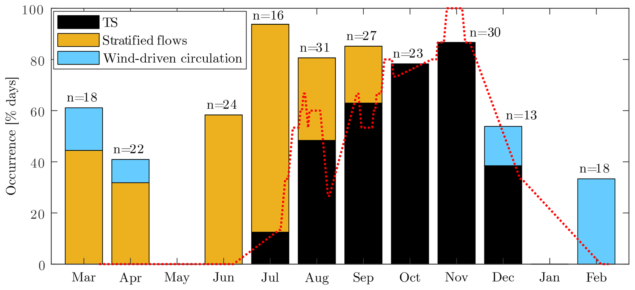
Figure 5 Monthly occurrence of TSs and other cross-shore (southwestward) flows at MT, expressed as a percentage of the days with measurements. The other cross-shore flows are divided between wind-driven circulation ($\mathrm{|}{L}_{\mathrm{MO}}\mathrm{|}/h_{\mathrm{ML}}>\mathrm{0.5}$) and stratified flows at MT ($\mathrm{d}T/\mathrm{d}z>\mathrm{0.05}$ ^∘C m⁻¹). The red dashed line indicates the 15 d moving average of the percentage of occurrence of TSs. The number of days with measurements (n) is shown for each month. Months with less than 10 d of measurements have been removed (May 2019 and January 2020).

The 15 d moving average in Fig. 5 reveals the short-term variability due to synoptic changes in the meteorological conditions that naturally modulate the seasonal pattern. Although the monthly averaged occurrence increases from August to November, the biweekly percentage of occurrence drops over shorter periods. These periods are associated with strong heating that re-stratifies the water column at MT, reduces surface cooling at night, and prevents TS formation (Appendix B, Fig. B1). The 15 d averaged occurrence reaches 100 % in November, when a TS is present over 25 consecutive days.

Although TSs become more frequent in autumn, the percentage of occurrence of cross-shore flows (p_CS) remains constant at around 80 %–90 % from July to November. Lateral flows observed at MT in spring and summer primarily result from direct wind forcing or subsequent stratified mixing. These flows may also include TSs intruding before reaching MT and, therefore, not counted as downslope TSs (further details in Appendix D). These different processes become less frequent in autumn due to the deeper mixed layer and are replaced by downslope TSs. Overall, there seems to be an effect of TSs on the number of cross-shore flows if we compare the period from July to December ($p_{\mathrm{CS}}\approx \mathrm{80}\pm \mathrm{14}$ %) with the rest of the year ($p_{\mathrm{CS}}\approx \mathrm{47}\pm \mathrm{12}$ %), suggesting that TSs are the main mechanism connecting the littoral and pelagic regions in Rotsee.

3.4 Scaling the cross-shore transport

We compare our field-based transport estimates for the TS events identified in Fig. 5 with the laboratory-based scaling formulae introduced in Sect. 2.6 (Fig. 6). The daily average and maximum cross-shore velocities are linearly correlated with the horizontal velocity scale from Eq. (9) (R²>0.5, $p_{\mathrm{val},\mathrm{F}}<\mathrm{0.01}$; Fig. 6a, b). The daily average velocity $U_{\mathrm{avg}}\approx \mathrm{0.9}\pm \mathrm{0.2}$ cm s⁻¹ is 3 times lower than the daily maximum velocity $U_{\max }\approx \mathrm{2.6}\pm \mathrm{0.7}$ cm s⁻¹ that occurs in the morning (Fig. 3). The best linear fits (with 0 intercept) are given by $U_{\mathrm{avg}}=\mathrm{0.33}\cdot (B_{\mathrm{0}}{L}_{\mathrm{ML}}{)}^{\mathrm{1}/\mathrm{3}}$ and $U_{\max }=\mathrm{0.99}\cdot (B_{\mathrm{0}}{L}_{\mathrm{ML}}{)}^{\mathrm{1}/\mathrm{3}}$. The 95 % confidence interval of the proportionality coefficient is $\mathrm{0.32}\le c_{\mathrm{U}}\le \mathrm{0.34}$ for U_avg and $\mathrm{0.95}\le c_{\mathrm{U}}\le \mathrm{1.02}$ for U_max. Despite the natural variability, a seasonal trend is distinguishable, with a decrease in U_avg and U_max by a factor of 2 from July to December. This is consistent with the weakening of convective cooling observed in Fig. 4.

Figure 6 (a) Daily averaged cross-shore velocity, (b) daily maximum cross-shore velocity, (c) daily averaged unit-width discharge, and (d) flushing timescale as a function of scaling formulae (Sect. 2.6). The equation of the linear regressions with 0 intercept, the coefficient of determination (R²), and the p value of an F test (p_val,F) are indicated.

The unit-width discharge q_avg and flushing timescale τ_F are also well predicted by the scaling formulae (Eqs. 10 and 11, respectively), despite a larger scatter than for the cross-shore velocity (R²≈0.2–0.3, $p_{\mathrm{val},\mathrm{F}}<\mathrm{0.01}$; Fig. 6c, d). The unit-width discharge $q_{\mathrm{avg}}\approx \mathrm{0.015}\pm \mathrm{0.004}$ m² s⁻¹ corresponds to an average thickness of $h_{\mathrm{TS},\mathrm{avg}}=q_{\mathrm{avg}}/U_{\mathrm{avg}}\approx \mathrm{1.8}\pm \mathrm{0.2}$ m and a flushing timescale of ${\mathit{\tau }}_{\mathrm{F}}\approx \mathrm{9.7}\pm \mathrm{2.7}$ h. The best relationships (with 0 intercept) are given by $q_{\mathrm{avg}}=\mathrm{0.34}\cdot (B_{\mathrm{0}}{L}_{\mathrm{ML}}{)}^{\mathrm{1}/\mathrm{3}}{h}_{\mathrm{lit}}$ (R²=0.27) and ${\mathit{\tau }}_{\mathrm{F}}=\mathrm{2.99}\cdot L_{\mathrm{lit}}/(B_{\mathrm{0}}{L}_{\mathrm{ML}}{)}^{\mathrm{1}/\mathrm{3}}$ (R²=0.18). The 95 % confidence interval of the proportionality coefficient is $\mathrm{0.33}\le c_q\le \mathrm{0.36}$ for q_avg and $\mathrm{2.83}\le c_{\mathrm{F}}\le \mathrm{3.15}$ for τ_F. The strong daily variability is explained by the fluctuating TS thickness during the convective period (Fig. 3c, d), which affects the calculation of the discharge (further details in Appendix D). As observed for the cross-shore velocity, the cross-shore transport weakens from summer to winter: q_avg decreases and τ_F increases by a factor of 2. The flushing timescale is τ_F≈7 h in summer but reaches τ_F≈20 h in winter. However, due to longer TS events in winter than in summer, the volume flushed by a single TS event is independent of the season and remains larger than the volume of the littoral region (Appendix C).

3.5 Flushing period

The diurnal cycle described in Sect. 3.1 varies at the seasonal scale, as the forcing parameters change. To assess the effects on the flushing period (period no. 3 in Fig. 3d), we average the diurnal cycle monthly between August and December (Fig. 7). The cooling and heating phases are illustrated with the diurnal cycle of B_0,net. The duration of the cooling phase (blue shading in Fig. 7) markedly increases from August to December, as already observed in Figs. 3a and 4b. The histograms of $\mathrm{|}{B}_{\mathrm{0},\mathrm{net}}^{\max }\mathrm{|}$ show that the magnitude of and variability in B_0,net decrease over the same period (Fig. 7b, d, f, h, j).

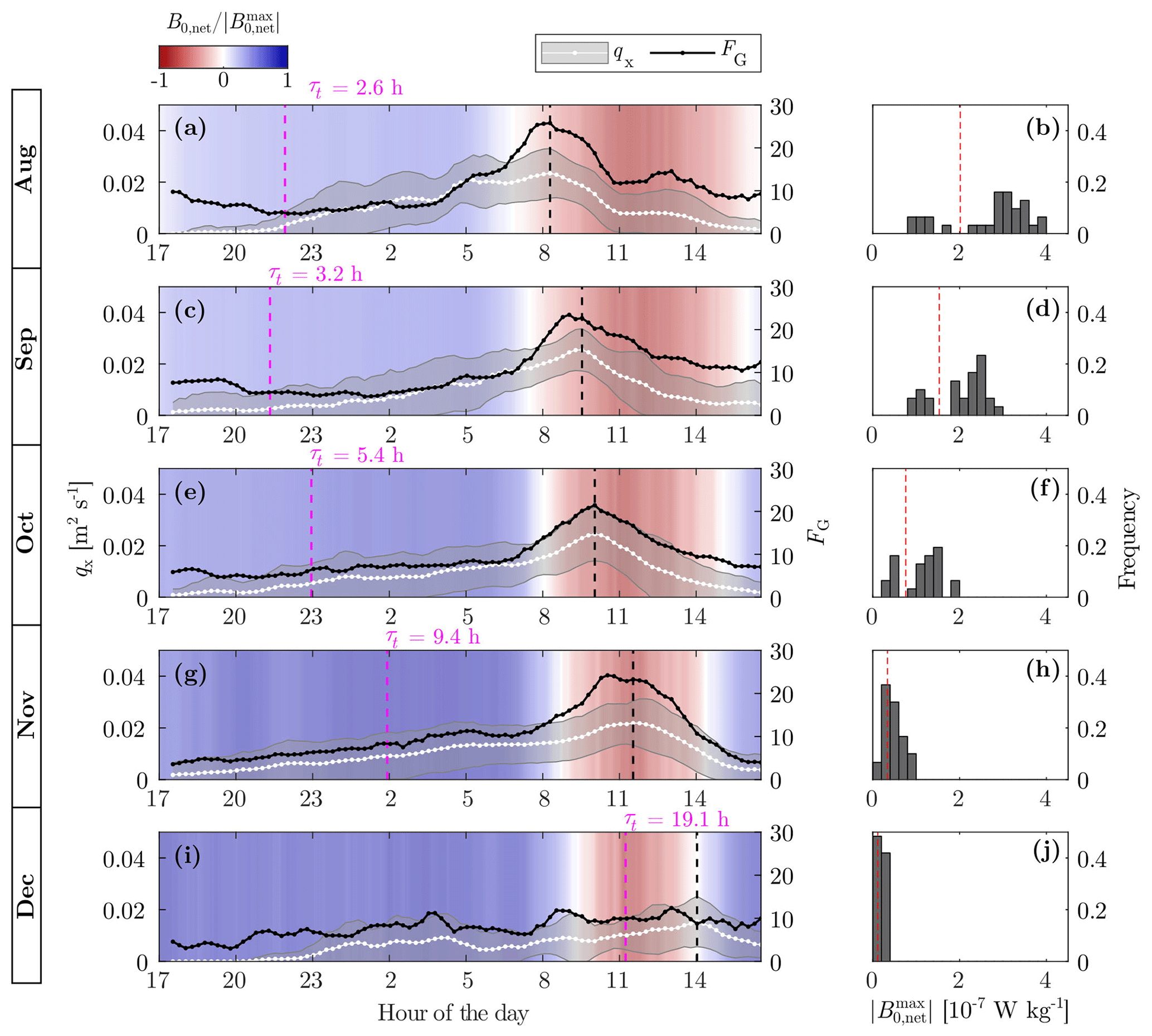
Figure 7 Seasonal variability in the diurnal cycle. (a, c, e, g, i) Monthly average of the diurnal cycle of the unit-width discharge q_x and F_G parameter. Only days with observed TSs between August and December have been averaged. The shaded white area corresponds to average discharge ± standard deviation. The monthly averaged net buoyancy flux represented as a color map is normalized by the maximum absolute value of each month. The vertical black dashed line indicates the time of maximal q_x. The transition timescale τ_t defines the starting time of the flushing, represented by a pink vertical dashed line. (b, d, f, h, j) Histograms of the maximum absolute value of the net buoyancy flux $\mathrm{|}{B}_{\mathrm{0},\mathrm{net}}^{\max }\mathrm{|}$ for each month. The red vertical line corresponds to $\mathrm{|}{B}_{\mathrm{0},\mathrm{net}}^{\max }\mathrm{|}$ of the monthly averaged diurnal cycles.

These changes in the forcing parameters have a direct effect on the cross-shore transport. The unit-width discharge in Fig. 7 (white dotted line) is obtained by monthly averaging the 24 h time series q_x(t). The discharge q_x(t) is calculated from Eq. (6) during the flushing period $t_{\mathrm{0}}\le t\le t_{\mathrm{f}}$ and q_x(t)=0 for t<t₀ or t>t_f. In August and September (Fig. 7a, b), q_x increases at night to reach its maximum at the beginning of the heating phase. The flow generally stops in the late morning, depicted by a drop in q_x at around 10:00 UTC. This cycle corresponds to the example in Fig. 3. The daily peak in flushing is also observed in October and November, but it is more spread with a continuous increase in cross-shore transport at night, which can already be seen in the evening (Fig. 7e, g). Thus, the average flushing duration of TSs is longer in late autumn (see, for example, the 24 h long TS event in Appendix B, Fig. B2). In December, the peak in discharge is reduced and the cross-shore transport is nearly continuous over 24 h (Fig. 7i). The time of maximal q_x (vertical black dashed line in Fig. 7) is delayed from August to December. We associate this maximal q_x with the heating phase, as it always occurs ∼1–2 h after B_0,net becomes negative (except in December, during which time the peak is less pronounced).

The diurnal cycle of the cross-shore transport is also described by the flow geometry parameter introduced by Ulloa et al. (2022) as the ratio between the root-mean-square (RMS) of the cross-shore velocity and the RMS of the vertical velocity:

$$\begin{array}{}\text{(13)}& F_{\mathrm{G}}\left(t\right)={\displaystyle \frac{\sqrt{〈U_x(t{)}^{\mathrm{2}}〉}}{\sqrt{〈U_z(t{)}^{\mathrm{2}}〉}}},\end{array}$$

where < … > denotes a depth average. F_G provides information on the relative magnitude of TSs with respect to the surface convection. We expect F_G to be close to unity when surface convection is the only process acting on the water column. A deviation from unity towards larger values of F_G (i.e., F_G≫1) implies that the flow is anisotropic, with a stronger cross-shore component, as a TS develops. A sharp peak in the monthly averaged F_G is visible at the beginning of the heating phase, from August to November (Fig. 7). It matches the time of maximal q_x and results from the combined effect of TS-induced flushing (increase in U_x) and convection weakening (decrease in U_z).

To give a theoretical estimation of the starting time of the flushing, we estimate the initiation timescale of TSs from the monthly averaged transition timescale τ_ini≈τ_t (Eq. 12). The assumption of constant surface cooling is reasonable for nighttime cooling in Rotsee (Fig. 3b). The starting time, depicted by a vertical pink dashed line in Fig. 7, corresponds to (t_sunset+τ_t), where t_sunset is the time of sunset when B_SW,0 drops to zero. The increase in τ_t from τ_t≈3 h in late summer to τ_t≈20 h in winter leads to a later theoretical onset of TSs in winter, despite the earlier time of sunset. Based on this seasonal variability in τ_t, TSs are expected to start in the evening in summer but in the morning in winter. This theoretical starting time, however, can be improved by considering the initial stratification at the beginning of the cooling phase, as further discussed in Sect. 4.2 and 4.4.

4 Discussion

4.1 Seasonality of thermal siphons

Our 1-year-long measurements show that both the occurrence and intensity of TSs vary seasonally in lakes with shallow littoral zones comparable to Rotsee. TSs occur regularly from late summer to early winter, with a maximum frequency in November, and are absent the rest of the year (Sect. 3.3). While the frequency of TSs increases in autumn, the intensity of the net cross-shore transport decreases compared with the summer period (Sect. 3.4). However, the daily averaged volume flushed from the littoral region increases from summer to autumn (Appendix C). The diurnal cycle is well defined in summer and divided into a cooling phase at night and a heating phase during daytime (Sect. 3.1). TSs form during the second part of the night and last until late morning, reaching a maximal flushing at the beginning of the heating phase. In autumn, the flushing duration increases, and the time of maximal flushing is shifted later in the day (Sect. 3.5).

To explain the TS seasonality, we need to relate it to the seasonal variability in the forcing parameters. The duration of the cooling phase (τ_c) is a key parameter to understand the TS occurrence and the diurnal dynamics, while the intensity of surface cooling (B₀) and the stratification (h_ML) parametrize the cross-shore transport. We discuss the effects of the forcing parameters on the TS seasonality in the following sections.

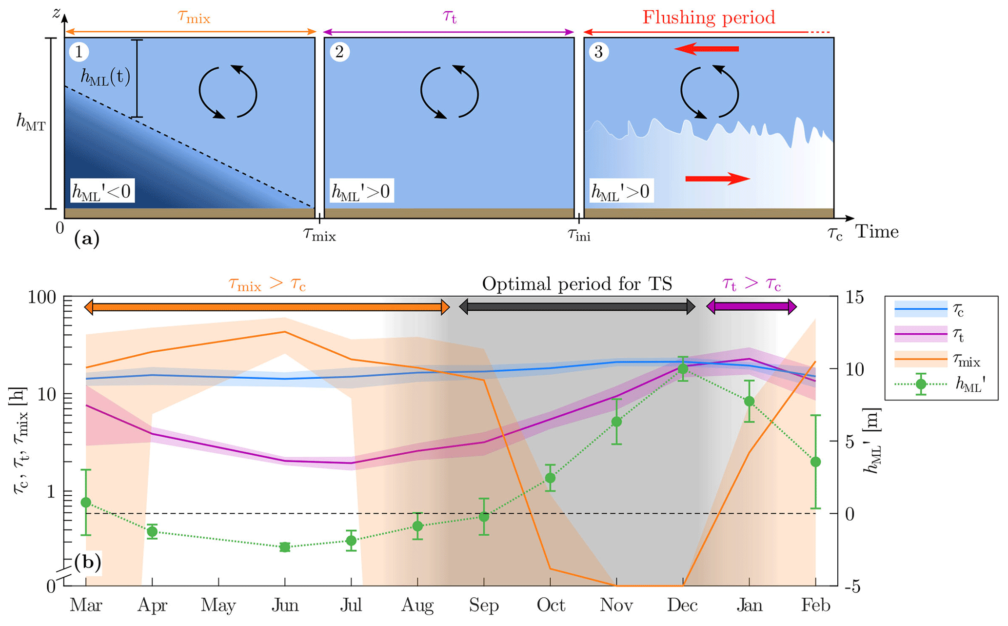
Figure 8 Timescales determining the occurrence of TSs. (a) Schematic of the three periods of the cooling phase at MT (Fig. 3d) parameterized by the mixing timescale τ_mix, transition timescale τ_t, and cooling duration τ_c. The mixed-layer depth is expressed as the relative depth $h_{\mathrm{ML}}^{\prime }=h_{\mathrm{ML}}-h_{\mathrm{MT}}$, with respect to h_MT=4 m. The mixed layer deepens during the first period ($\mathrm{0}<t<{\mathit{\tau }}_{\mathrm{mix}}$), until the complete mixing of the water column. The transition period (${\mathit{\tau }}_{\mathrm{mix}}<t<{\mathit{\tau }}_{\mathrm{ini}}$) is dominated by convection. TSs occur during the flushing period (${\mathit{\tau }}_{\mathrm{ini}}<t<{\mathit{\tau }}_{\mathrm{c}}$). (b) Effects of the seasonality of τ_mix, τ_t, τ_c, and $h_{\mathrm{ML}}^{\prime }$ on the TS occurrence. Monthly averages are represented, with shaded areas (τ_c, τ_t, and τ_mix) and error bars ($h_{\mathrm{ML}}^{\prime }$) indicating the monthly standard deviation. Note the log scale for the axis of timescales. The gray shaded period corresponds to optimal conditions for the TS occurrence.

4.2 Effects of the forcing parameters on the occurrence of thermal siphons

TS occurrence can be predicted by estimating the initiation timescale τ_ini and comparing it with the duration of the cooling phase (τ_c). A TS will occur if the cooling phase is long enough, i.e., τ_c>τ_ini. In initially stratified surface waters, the initiation period is divided into (1) a stratified period, during which the mixed layer deepens, and (2) a transition period, during which the littoral region is vertically mixed (Figs. 3d, 8a). We express the initiation timescale as ${\mathit{\tau }}_{\mathrm{ini}}={\mathit{\tau }}_{\mathrm{mix}}+{\mathit{\tau }}_{\mathrm{t}}$, where τ_mix is the time needed to vertically mix the littoral region, and τ_t is the transition timescale given by Eq. (12). To estimate τ_mix, we use the deepening rate of the mixed layer (Zilitinkevĭc, 1991) as follows:

$$\begin{array}{}\text{(14)}& {\displaystyle \frac{\mathrm{d}{h}_{\mathrm{ML}}}{\mathrm{d}t}}=(\mathrm{1}+\mathrm{2}A){\displaystyle \frac{B_{\mathrm{0}}}{h_{\mathrm{ML}}{N}^{\mathrm{2}}}}\left[\mathrm{m}{\mathrm{s}}^{-\mathrm{1}}\right],\end{array}$$

where $N^{\mathrm{2}}=-(g/\stackrel{\mathrm{‾}}{\mathit{\rho }})(\mathrm{d}\mathit{\rho }/\mathrm{d}z)$ [s⁻²] is the squared buoyancy frequency below the mixed layer, $\stackrel{\mathrm{‾}}{\mathit{\rho }}$ is the depth-averaged water density, and A≈0.2 is an empirical coefficient. The model of Eq. (14) assumes that the mixed layer deepens by convection only, without any wind contribution. This assumption is valid for calm conditions, which prevail in Rotsee due to wind sheltering (Zimmermann et al., 2021). The average duration required for mixing the water column at MT, assuming a constant surface cooling B₀ and an initial mixed-layer depth h_ML,ini, can be derived from Eq. (14) as follows:

$$\begin{array}{}\text{(15)}& {\mathit{\tau }}_{\mathrm{mix}}=\left(h_{\mathrm{MT}}^{\mathrm{2}}-h_{\mathrm{ML},\mathrm{ini}}^{\mathrm{2}}\right){\displaystyle \frac{N^{\mathrm{2}}}{\mathrm{2}{B}_{\mathrm{0}}(\mathrm{1}+\mathrm{2}A)}}\left[\mathrm{s}\right].\end{array}$$

In Eq. (15), the buoyancy frequency squared is approximated as $N^{\mathrm{2}}=-(g/\stackrel{\mathrm{‾}}{\mathit{\rho }})\left[\mathit{\rho }\right(z=-h_{\mathrm{ML},\mathrm{ini}})-\mathit{\rho }(z=-h_{\mathrm{MT}}\left)\right]/[h_{\mathrm{MT}}-h_{\mathrm{ML},\mathrm{ini}}]$. The depth h_MT corresponds to the maximum depth of the littoral region upslope of MT (Fig. 1), which has to be mixed to observe downslope TSs at MT.

From the seasonality of the forcing parameters (Fig. 4), we predict the optimal period for the TS occurrence based on τ_ini (Fig. 8b). In summer, the shallow mixed layer (h_ML≈2 m) and strong nighttime surface cooling ($B_{\mathrm{0}}\approx {\mathrm{10}}^{-\mathrm{7}}$ W kg⁻¹) lead to a short transition timescale of ${\mathit{\tau }}_{\mathrm{t}}\approx \mathrm{2}\pm \mathrm{0.5}$ h. However, the strong stratification near the surface limits the deepening of the mixed layer and causes τ_mix to be too large for the water column to mix at MT (orange period in Fig. 8b). The littoral region remains stratified for most of the nights (h_ML<h_MT), and the occurrence of downslope TSs at MT is low (τ_ini>τ_c on average). Downslope TSs start to be observed in late summer when the mixed layer reaches h_MT before the end of the night. Starting in October, the monthly averaged mixed layer is deeper than h_MT, and τ_mix≈0. At the same time, τ_t increases because of the deepening of the mixed layer and the decrease in B₀. The transition timescale becomes longer than τ_c in winter (purple period in Fig. 8b), reaching its maximum of ${\mathit{\tau }}_{\mathrm{t}}\approx \mathrm{23}\pm \mathrm{7}$ h in January. This prevents TSs from forming in winter, except for days with continuous surface cooling (i.e., τ_c>24 h). The transition timescale decreases in spring, but τ_mix increases simultaneously due to the re-stratification of the littoral region, which prevents TSs from occurring. Thus, the conditions to observe downslope TSs at MT are optimal between September and December, when τ_ini≪τ_c (gray shaded period in Fig. 8b). This period coincides well with our frequent observations of TSs in autumn. The limiting factor for the formation of TSs in spring and summer is τ_mix, whereas it is τ_t in winter.

During the optimal period of occurrence, the variability in forcing conditions (B_0,net) between days can modify the occurrence condition τ_ini<τ_c at a shorter timescale than the seasonal scale. Days with TSs are characterized by higher B_0,net than days without TSs (Appendix B, Fig. B1). This results in the short-term variability in the biweekly averaged occurrence in Fig. 5. Other mechanisms affect the TS occurrence on a daily basis, such as wind events. Direct wind forcing either enhances or suppresses TSs. We identified several wind events from September to December that prevented any flow in the offshore direction (i.e., no significant flow detected by the algorithm) or, conversely, generated a strong cross-shore circulation (wind-driven circulation in Fig. 5).

Although the TS occurrence over short periods may vary from one year to another, we expect the seasonal trend previously described to be repeated every year in Rotsee. We also suggest that a similar trend should be common in other temperate lakes. Most of the TS events reported for other systems were observed in late summer or autumn, corresponding to the occurrence period for Rotsee (Monismith et al., 1990; James and Barko, 1991a, b; James et al., 1994; Rogowski et al., 2019). James and Barko (1991b) showed that the percentage of days with differential cooling in Eau Galle Reservoir (WI, USA) increased from 31 % in May to 95 % in August. However, these high values do not correspond to the percentage of occurrence of TSs, as differential cooling can happen without necessarily forming a cross-shore circulation. Pálmarsson and Schladow (2008) also found that differential cooling was rare in May and June in Clear Lake (CA, USA). Only 2 nights were cold enough to result in cooling-driven TSs. In winter, TS events are not frequent in Rotsee, but they have been reported for larger systems such as Lake Geneva in January (Thorpe et al., 1999; Fer et al., 2002a, b). A different bathymetry modifies τ_t (Eq. 12), which becomes shorter if $h_{\mathrm{p}}/h_{\mathrm{ML}}$ is small or the slope is high, leading to a more frequent TS occurrence in winter. In addition, convective cooling stops earlier in small lakes like Rotsee that reach the temperature of maximum density before larger and deeper lakes.

4.3 Effects of the forcing parameters on cross-shore transport

The seasonality of the cross-shore transport induced by TSs can be examined using the scaling for the cross-shore velocity U_x (Eq. 9) and the unit-width discharge q_x (Eq. 10). The timescale τ_F is also a key parameter to assess the seasonality of the littoral region flushing (Eq. 11). We showed that these scaling formulae reproduce the observed seasonality in Rotsee (Fig. 6). The weakening of the transport from summer to winter is explained by the decrease in B₀ by a factor of 10, which overcomes the increase in L_ML due to the deepening of the mixed layer (Fig. 4). However, τ_F remains shorter than the duration of the cooling phase (Fig. 8b), and the littoral region upslope of MT (V_lit≈500 m²) is entirely flushed by a single event (Appendix C). The use of the constant length scale h_lit in Eq. (10) implies that the daily averaged TS thickness, $h_{\mathrm{TS},\mathrm{avg}}=q_{\mathrm{avg}}/U_{\mathrm{avg}}$, should not show any seasonal variability. We observe the following in Rotsee: h_TS,avg remains close to its yearly average of 1.8±0.2 m, without any seasonal trend.

Table 2 Comparison of the transport scaling formula $q=c_{q}h(B_{\mathrm{0}}L{)}^{\mathrm{1}/\mathrm{3}}$ between different studies on sloping basins, where h is a vertical length scale, and L is a horizontal length scale. The different notations can be found in Fig. 1 and Table 1. The littoral region is based on the location of the discharge measurement, as in Fig. 1. L_forc is the length over which the destabilizing forcing B₀ applies.

We further compare our scaling for U_x, q_x, and τ_F with previous studies on buoyancy-driven flows. The velocity scale $U\sim (B_{\mathrm{0}}L{)}^{\mathrm{1}/\mathrm{3}}$ from Phillips (1966) is commonly used, with L defined as the horizontal length scale along which a lateral density gradient is set. This length scale varies with the experimental configuration and basin geometry (Table 2). In laboratory experiments with a localized buoyancy loss, L is the length along which the destabilizing buoyancy flux applies (Harashima and Watanabe, 1986; Sturman et al., 1996; Sturman and Ivey, 1998). For more realistic systems undergoing uniform surface cooling, L is the length of the littoral region, which can be defined as the plateau zone (Ulloa et al., 2022) or the region vertically mixed by convection (Wells and Sherman, 2001). In the first case, L=L_p is a constant, whereas L=L_ML varies with the stratification in the second case. We chose to use L_ML because it corresponds to the region affected by differential cooling. We expect that a deeper mixed layer will increase the temperature difference ΔT between the littoral and pelagic regions, resulting in a higher velocity U_x. In Eqs. (10) and (11), the transport is expressed as a function of the velocity scale and the size of the littoral region of length L_lit and depth h_lit (Fig. 1). We defined the littoral region based on the location of MT because we measured the discharge out of this region. This definition of h_lit in Eq. (10) is consistent with the fact that q_x varies spatially, increasing with distance from the shore (Fer et al., 2002b). The vertical length scale h can also be chosen as the depth of the plateau (h_p) (Sturman and Ivey, 1998; Wells and Sherman, 2001; Fer et al., 2002b; Ulloa et al., 2022) to predict the discharge from the plateau region only. Despite these different choices of length scales, the coefficient c_q≈0.34 is close to other estimates from the literature (Table 2). Harashima and Watanabe (1986) found that c_q increases with the flux Reynolds number defined as $R{e}_{\mathrm{f}}=B_{\mathrm{0}}^{\mathrm{1}/\mathrm{3}}{h}_{\mathrm{lit}}^{\mathrm{2}}/\left[L_{\mathrm{ML}}^{\mathrm{2}/\mathrm{3}}\mathit{\nu }\right]$, where $\mathit{\nu }\approx \mathrm{1.5}\times {\mathrm{10}}^{-\mathrm{6}}$ m² s⁻¹ is the kinematic viscosity of water. The empirical relationship $c_q\approx \mathrm{0.43}-\mathrm{1.67}/R{e}_{\mathrm{f}}^{\mathrm{1}/\mathrm{2}}$ was obtained for Re_f>50. For the days where TSs are observed in Rotsee, Re_f varies from 250 in summer to 50 in winter, with an average value of ∼140 which leads to c_q≈0.29, close to our estimate of c_q≈0.34.

4.4 Effects of the forcing parameters on the flushing period

The seasonality of the forcing parameters does not only affect the occurrence and magnitude of TSs but also the diurnal dynamics of the littoral flushing (Fig. 7). The initiation of TSs always occurs several hours after the beginning of the cooling phase. This delay is modulated by τ_ini and is consistent with previous studies reporting the formation of a TS at night (Monismith et al., 1990; James et al., 1994; Fer et al., 2002b; Pálmarsson and Schladow, 2008) or in the morning (Rogowski et al., 2019; Sturman et al., 1999). τ_t is a good estimate of the initiation period when the water column is initially mixed (τ_mix=0). In summer and on warm autumn days, however, the initiation of TSs occurs later than predicted by τ_t, due to the initial stratification at the beginning of the cooling phase (τ_mix≠0). This leads to a delay in the increase in q_x and F_G (Fig. 7a, c). In autumn, TS events lasting for more than 24 h lead to monthly averaged q_x>0 before the starting time predicted by τ_t (Fig. 7e, g). In winter, τ_t→24 h implies that the rare TS events are all characterized by a continuous flow (Fig. 7i), without any diurnal cycle of flushing.

When a diurnal cycle is present in summer and autumn, the flushing period ends several hours after the beginning of the heating phase (Figs. 3, 7). This inertia has already been reported by Monismith et al. (1990), who observed TSs until the mid-afternoon, despite the opposite pressure gradients due to differential heating. In addition to the delay between the end of the cooling and the end of the flow, we also showed that a peak in flushing occurred a few hours after the beginning of the heating phase (Fig. 3). The time of maximal flushing is shifted later in the day from summer to winter, as the heating phase starts later (Fig. 7). The maximal flushing seems related to the transition from the cooling phase to the heating phase. This finding suggests that convective plumes eroding the flow control the weak initial transport during the cooling phase. A weakening of convection reduces this vertical mixing and finally enables the flushing to reach its maximum intensity. Further investigations are required to better understand this process.

4.5 Practical recommendations to predict and measure thermal siphons in other lakes

Rotsee is an ideal field-scale laboratory to investigate TSs, due to wind sheltering and its elongated shape minimizing complex recirculation. To assess the TS seasonality in other lakes, long-term velocity and temperature measurements in the sloping region are required. The developed algorithm to detect TS events (Sect. 2.4) and calculate the cross-shore transport (Sect. 2.5) fulfilled our requirements but remained lake-specific. The limitations of the algorithm are discussed in more detail in Appendix D. The general structure of the algorithm (Sect. 2.4) can serve as a basis for detecting TSs in lakes, by adapting the lake-specific criteria to other systems. The 2D framework of TSs requires specific validation in more complex nearshore systems and large lakes, where the topography, large-scale circulation, and Coriolis may also affect the TS dynamics (Fer et al., 2002b). In these systems, the alongshore velocity component of TSs must be considered in the cross-shore transport analysis. Further development is needed to build a more robust algorithm with lake-independent physically based criteria.

The effects of a different bathymetry can be predicted from the scaling discussed in the previous sections. A shallower nearshore plateau region or a steeper sloping region would decrease the transition timescale τ_t (Eq. 12), causing the initiation of TSs to happen earlier and more often. Higher slopes would also decrease the length of the mixed region L_ML and reduce the horizontal velocity of TSs (Eq. 9). Past observations of TSs have reported horizontal velocities ranging from ∼0.1 cm s⁻¹ (James and Barko, 1991a, b) to ∼10 cm s⁻¹ (Roget et al., 1993; Fer et al., 2002b), with U_x∼1 cm s⁻¹ in most cases (Monismith et al., 1990; Sturman et al., 1999; Pálmarsson and Schladow, 2008; Rogowski et al., 2019). The cross-shore transport q_x and flushing timescale τ_F are strongly dependent on the size and depth of the littoral region considered (Eqs. 10, 11). A deeper littoral region (larger h_lit) would lead to a stronger discharge, and a longer littoral region (larger L_lit) would take more time to flush. Values of TS thickness and discharge can be 1 order of magnitude larger in lakes deeper than Rotsee (Thorpe et al., 1999; Fer et al., 2002a; Rogowski et al., 2019). The effects of more complex bathymetries, departing from our 2D framework, could be further investigated with 3D numerical simulations.

Information on lake bathymetry and thermal structure are needed to predict the occurrence (τ_ini<τ_c) and intensity of TSs (U_x, q_x, τ_F) under specific forcing. This approach does not consider wind effects, which deserve further investigation. Windier conditions would hinder TSs by locally enhancing and reducing the cross-shore transport. In this case, the scaling formulae (Eqs. 9–11) should be modified to take wind shear into account. The littoral region would also be mixed faster under windy conditions, and the effects of wind mixing on τ_mix should be included in Eq. (15). These questions could be addressed by performing numerical simulations with varying wind speed.

The TS seasonality may evolve in a changing climate, which also needs to be investigated. Changes in heat fluxes, summer stratification, and surface temperature would affect both the intensity (B₀) and occurrence (τ_ini) of TSs.

5 Conclusions

The flushing of the littoral region by cross-shore flows increases the exchange between nearshore and pelagic waters. In this study, we investigated one of the processes that enhance the renewal of littoral waters, the so-called thermal siphon (TS) driven by differential cooling. From a 1-year-long monitoring of TSs in a small, temperate, wind-sheltered lake, we quantified the seasonality of the cross-shore transport induced by TSs. This seasonality is related to the intensity of surface cooling (surface buoyancy flux B₀) and the lake stratification (mixed-layer depth h_ML). Three aspects of the TS seasonality are highlighted. First, TSs are a recurring process from late summer to winter (when τ_c>τ_ini), occurring on ∼80 % of autumn days. Second, the seasonal changes in the TS-induced transport are well reproduced by the scaling $U_{\mathrm{avg}}\approx \mathrm{0.33}\cdot (B_{\mathrm{0}}{L}_{\mathrm{ML}}{)}^{\mathrm{1}/\mathrm{3}}$, $q_{\mathrm{avg}}\approx \mathrm{0.34}\cdot (B_{\mathrm{0}}{L}_{\mathrm{ML}}{)}^{\mathrm{1}/\mathrm{3}}{h}_{\mathrm{lit}}$, and ${\mathit{\tau }}_{\mathrm{F}}=V_{\mathrm{lit}}/q_{\mathrm{avg}}\approx \mathrm{2.99}\cdot L_{\mathrm{lit}}/(B_{\mathrm{0}}{L}_{\mathrm{ML}}{)}^{\mathrm{1}/\mathrm{3}}$, where L_ML is the length of the region mixed by convection, and V_lit=L_lith_lit is the unit-width volume of the littoral region. This study provides a field validation of this laboratory and theoretically based scaling. Third, the diurnal dynamics of the flushing follow the seasonal changes in the cooling and heating phases, by evolving from a well-defined diurnal cycle in summer to a more continuous flow in winter.

Our results demonstrate that TSs significantly contribute to the flushing of the nearshore waters. This process occurs frequently during the cooling season (>50 % of the time), each time flushing the entire littoral region. We stress that this buoyancy-driven transport is, perhaps counterintuitively, stronger in summer and in the morning. Such a timing has implications for the transport of dissolved compounds, with, for instance, maximal exchange between littoral and pelagic waters at a time of high primary production (summer and daytime). Overall, this study provides a solid framework to integrate the role of TSs in the lake ecosystem dynamics.

Appendix A: Instrumentation

Table A1 Specifications and setup of the sensors from the two moorings and the meteorological station. For the ADCP, only the complete days of measurements used for the transport estimates are taken into account in the measurement periods.

Appendix B: Diurnal variability in the occurrence and duration of thermal siphons

In addition to the seasonality, TSs also vary between days. A change in forcing conditions (B_0,net) between days may enhance or prevent TS formation, by modifying the occurrence condition τ_ini<τ_c at a short timescale. We average the net buoyancy flux over 48 h ($B_{\mathrm{0},\mathrm{net}}^{\mathrm{2}\mathrm{d}}$), for each 24 h subset starting at 17:00 UTC. $B_{\mathrm{0},\mathrm{net}}^{\mathrm{2}\mathrm{d}}$ is the average of B_0,net between 00:00 UTC on the first day of the 24 h subset and 23:59 UTC on the following day. This quantity includes the effects of the forcing on (1) the initial stratification, which affects τ_ini (day preceding the TS event), and (2) the duration of the cooling phase τ_c (following day). We compare the values of $B_{\mathrm{0},\mathrm{net}}^{\mathrm{2}\mathrm{d}}$ between days with and without TSs (Fig. B1). Days with TSs are characterized by higher $B_{\mathrm{0},\mathrm{net}}^{\mathrm{2}\mathrm{d}}$ than days without TSs, which is confirmed by a t test at a 5 % significance level, from August to December. The variability in the forcing conditions between days also affects the flushing duration of TSs (Fig. B2).

Figure B1 Box plots of the 2 d averaged net surface buoyancy flux for each month, depending on the occurrence of TS events.

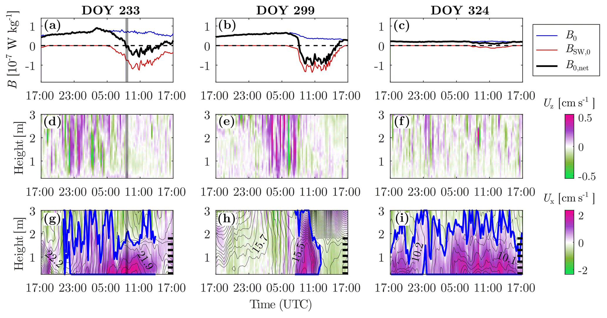
Figure B2 Three examples of TS events, with (a–c) buoyancy fluxes, (d–f) vertical velocity, and (g–i) cross-shore velocity, as in Fig. 3. (a, d, g) A long TS event on 21–22 August 2019 due to short heating phases on both days. (b, e, h) A short TS event on 26–27 October 2019 due to strong heating on both days (re-stratification). (c, f, i) Continuous flushing on 20–21 November 2019 due to continuous net cooling. See the caption of Fig. 3 for more details about each panel. The gray shaded area in panels (a), (d), and (g) indicates the time of the CTD transect shown in Fig. 1.

Appendix C: Seasonality of the flushing of the littoral region

The unit-width volume flushed by each TS event is calculated by integrating the discharge q_x over the flushing period (Eq. 5). We estimate the daily averaged flushed volume V_flush,day and the averaged flushed volume of TS events V_flush,TS by dividing the total volume of water flushed every month by the number of days with measurements and by the number of days with TSs, respectively. The volume V_flush,day includes the effect of the occurrence of TS events on the daily flushing, whereas V_flush,TS only depends on the intensity and duration of a TS event. We express both flushed volumes as fractions of the littoral region of volume V_lit (Fig. C1). The seasonal trend of V_flush,day is similar to the TS occurrence (Fig. 5), with an increase in flushing from July to November (Fig. C1a). This indicates that the increase in the TS occurrence from summer to autumn overcomes the weakening of the transport over the same period. The flushed volume of TS events does not vary significantly with season (Fig. C1b). A single TS event flushes the littoral region more than once on average. Overall, the TS occurrence is the primary factor controlling the seasonality of the littoral flushing in Rotsee.

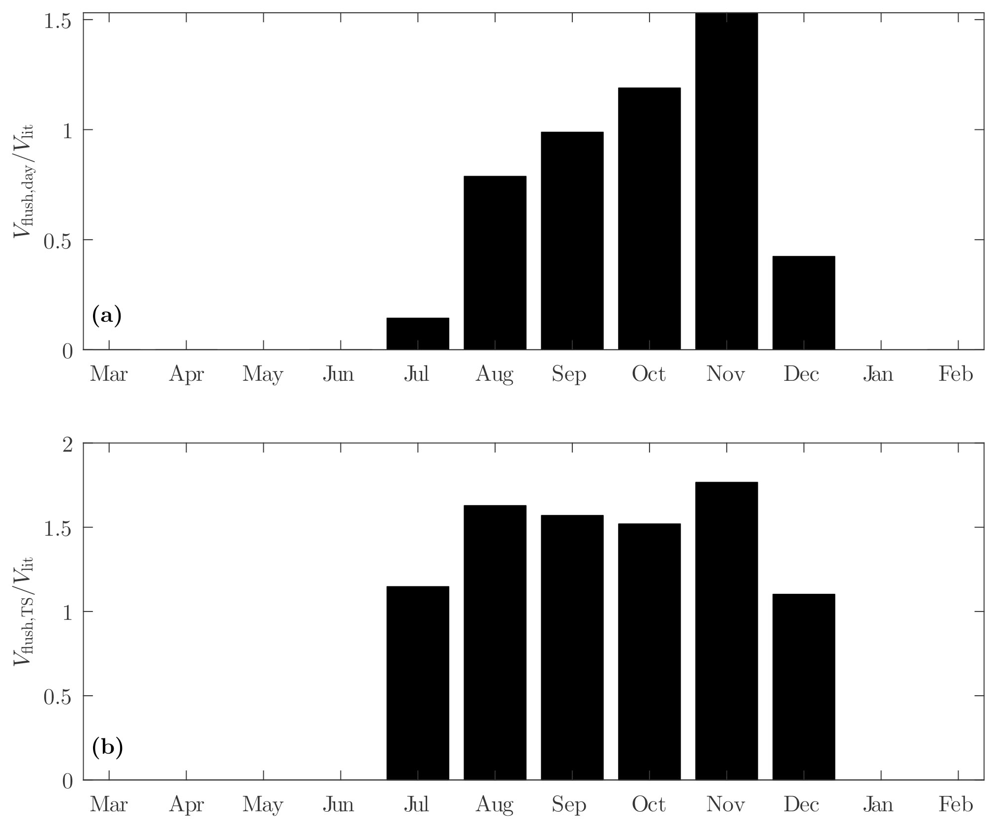
Figure C1 Fraction of the littoral region flushed by TSs in 1 d for each month. Months with less than 10 d of measurements have been removed as in Fig. 5 (May 2019 and January 2020). (a) The daily averaged flushed fraction including all days with measurements. (b) The daily averaged flushed fraction for days with TSs only.

Appendix D: Identification of thermal siphons by the algorithm

The developed algorithm used to detect TS events (Sect. 2.4) and calculate the cross-shore transport (Sect. 2.5) aimed at automatizing the identification of TSs and, thus, at limiting subjective bias in the characterization of the process. We manually assessed the performance of the algorithm over different days. We further tested the validity of the identified TS events with the fact that a cross-shore transport resulting from a TS should be associated with a decrease in water temperature (Fig. 1). We calculated the correlation r(U_x,T) between the cross-shore velocity U_x and the temperature T from the thermistor array at MT, at each depth and during the cross-shore flow events. The negative correlation during 93 % of the identified TS events ($r(U_x,T)<-\mathrm{0.48}$ according to the 95 % confidence interval from a t test) and the lack of clear negative correlation (at a 5 % significance level) during the other days justified the skills of the detection algorithm. The general structure of the algorithm can be used in other systems. However, several criteria are lake-specific and must be adapted to the system of interest. We discuss the limitations of the algorithm below and provide suggestions for improvement.

The definition of a significant cross-shore flow by the algorithm (i.e., $\stackrel{\mathrm{‾}}{U_x}>\mathrm{0.5}$ cm s⁻¹ for at least 2 h) is lake-specific. This criterion is based on typical examples of TSs in Rotsee, where $\stackrel{\mathrm{‾}}{U_x}$ is above 0.5 cm s⁻¹ over most of the flushing period. Theoretical estimates of the period between the onset time and the end of the cooling phase (e.g., ${\mathit{\tau }}_{\mathrm{c}}-{\mathit{\tau }}_{\mathrm{ini}}\approx \mathrm{10}$ h in autumn) show that most TS events last more than 2 h and justify the chosen threshold for the duration. From a sensitivity analysis (Fig. D1), we notice that the TS occurrence does not change significantly if the duration threshold is increased by a few hours. Shorter cross-shore flow events must be discarded because they are not consistent with the gravitational adjustment triggered by differential cooling; they could be wind-driven or result from free surface convection. In Rotsee, cross-shore flows driven by internal waves are expected to be short and to be discarded by the algorithm ($T_{\mathrm{V}\mathrm{1}\mathrm{H}\mathrm{1}}/\mathrm{2}\approx \mathrm{2.5}$ h in summer, where T_V1H1 is the period of V1H1 internal waves). Other types of data could be included to detect TSs, such as lateral temperature gradients, near-surface velocity (return flow), or vertical velocity (convective plumes). Using other techniques, like machine learning algorithms, could also be a useful approach to better identify TS events.

Figure D1 Sensitivity analysis for the criteria used to define cross-shore flows. The effects of modifying the depth-averaged cross-shore velocity $\stackrel{\mathrm{‾}}{U_x}$ and the averaging duration Δt are shown as changes in the percentage of occurrence of TSs (p_TS) for each month. Δp_TS is the percentage difference with respect to the occurrence shown in Fig. 5, obtained with $\stackrel{\mathrm{‾}}{U_x}=\mathrm{0.5}$ cm s⁻¹ and Δt=2 h (reference point shown by the red cross).

The filter used to discard days with wind-driven circulation is based on the criterion $\mathrm{|}{L}_{\mathrm{MO}}\mathrm{|}/h_{\mathrm{ML}}={\mathit{\kappa }}^{-\mathrm{1}}\mathrm{|}{u}_{*}/w_{*}{\mathrm{|}}^{\mathrm{3}}>\mathrm{0.5}$, where κ=0.41 is the von Kármán constant, and u_* the friction velocity. The ratio $u_{*}/w_{*}$ expresses the relative importance of wind shear compared with convection. The threshold value of 0.5 was successfully tested on wind-driven circulation events observed in Rotsee in winter. This filter discards the strongest wind events, but cross-shore flows with $\mathrm{|}{L}_{\mathrm{MO}}\mathrm{|}/h_{\mathrm{ML}}<\mathrm{0.5}$ can still be affected by a wind peak during the flushing period (e.g., interaction between wind and a TS). Being more conservative and decreasing the threshold value from 0.5 to 0.1 would discard TS events mainly in December (when w_* is low) but would not significantly modify the TS occurrence during the other periods (Fig. D2). Additional filters could be implemented to distinguish between TSs and wind-driven cross-shore flows, based, for example, on high-resolution vertical velocity measurements, observed oscillations of the thermocline (e.g., wavelet analysis), estimates of the period of internal waves, and identification of upwelling events (e.g., Wedderburn and Lake numbers) (Imberger and Patterson, 1989).

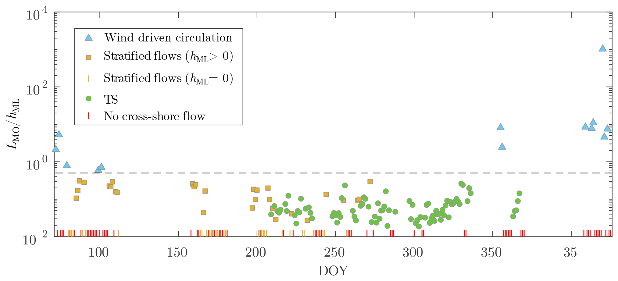
Figure D2 Filtering of the 227 d analyzed, shown as a time series of $L_{\mathrm{MO}}/h_{\mathrm{ML}}$ from March 2019 to March 2020. Days without a significant cross-shore flow or without a mixed layer are depicted as bottom ticks. Stratified flows are cross-shore flows without complete mixing at MT. The wind-driven circulation threshold $L_{\mathrm{MO}}/h_{\mathrm{ML}}=\mathrm{0.5}$ is shown by the horizontal dashed line.

By discarding days with stratified conditions at MT, the second filter does not consider TSs that intrude before reaching MT and appear as interflows. Thus, TS occurrence in summer is underestimated. In Fig. 5, the higher percentage of occurrence of stratified flows in July (81 %) compared with spring (around 40 %–50 %) suggests a possible contribution of intruding TSs. From visual inspection of each event, we estimated that intruding TSs could represent almost half of the stratified flows in July. Including downslope TSs only was relevant, as the transport properties of interflows can be different from downslope gravity currents, for which the scaling formulae were derived. In addition, intruding TS events could be confounded with other baroclinic flows, and further filtering steps would have been required to detect them correctly.

The transport quantities of TSs are averaged over the flushing period (Sect. 2.5). The onset of the flushing is challenging to define because of the interaction between TSs and convective plumes (Fig. 3c). The cross-shore velocity field can be very variable over time, with vertical fluctuations of the region with positive U_x (Fig. 3d). We decided to include only the period over which the region with positive U_x remained at the same depths (i.e., the limits of the flushing period correspond either to vertical displacements of the region of positive U_x or to U_x≤0 at all depths). This approach might sometimes include only a part of the TS event in the transport calculations. Daily averaged velocities should not be affected. The average thickness and discharge, however, vary between days depending whether the vertical oscillations of the TS interface are included or not. The latter is a possible reason for the larger variability observed for q_avg and τ_F (Fig. 6).