the Creative Commons Attribution 4.0 License.
the Creative Commons Attribution 4.0 License.
 | 15 Jun 2022
A two-step merging strategy for incorporating multi-source precipitation products and gauge observations using machine learning classification and regression over China
Huajin Lei
Hongyu Zhao
Tianqi Ao
Although many multi-source precipitation products (MSPs) with high spatiotemporal resolution have been extensively used in water cycle research, they are still subject to various biases, including false alarm and missed bias. Precipitation merging technology is an effective means to alleviate this uncertainty. However, how to efficiently improve precipitation detection efficiency and precipitation intensity simultaneously is a problem worth exploring. This study presents a two-step merging strategy based on machine learning (ML) algorithms, including gradient boosting decision tree (GBDT), extreme gradient boosting (XGBoost), and random forest (RF). It incorporates six state-of-the-art MSPs (GSMaP, IMERG, PERSIANN-CDR, CMORPH, CHIRPS, and ERA5-Land) and rain gauges to improve the accuracy of precipitation identification and estimation from 2000 to 2017 over China. Multiple environment variables and spatial autocorrelation are combined in the merging process. The strategy first employs classification models to identify wet and dry days and then combines regression models to predict precipitation amounts based on classified wet days. The merged results are compared with traditional methods, including multiple linear regression (MLR), ML regression models, and gauge-based Kriging interpolation. A total of 1680 (70 %) rain gauges are randomly chosen for model training and 692 (30 %) for performance evaluation. The results show that (1) the multi-source merged precipitation products (MSMPs) outperformed all original MSPs in terms of statistical and categorical metrics, which substantially alleviates the temporal and spatial biases. The modified Kling–Gupta efficiency (KGE), critical success index (CSI), and Heidke Skill Score (HSS) of original MSPs are improved by 15 %–85 %, 17 %–155 %, and 21 %–166 %, respectively. (2) The spatial autocorrelation plays a significant role in precipitation merging, which considerably improves the model accuracy. (3) The performance of MSMPs obtained by the proposed method is superior to MLR, Kriging interpolation, and ML regression models. The XGBoost algorithm is recommended more for large-scale data merging owing to its high computational efficiency. (4) The two-step merging strategy performs better when higher-density gauges are used to model training. However, it has strong robustness and can also obtain better performance than original MSPs even when the gauge number is reduced to 10 % (237). This study provides an accurate and reliable method to improve precipitation detection accuracy under complex climatic and topographic conditions. It could be applied to other areas well if rain gauges are available.
- Article
(13487 KB) - Full-text XML
- BibTeX
- EndNote


As one of the critical parameters of the natural water cycle, precipitation helps us realistically understand the interaction between hydrological and climate systems. Moreover, precipitation monitoring is essential for forecasting of extreme hydroclimatic disasters and for management of water resources (Yilmaz et al., 2005; Tao et al., 2016; Xu et al., 2018). Accurate precipitation estimates are of practical importance for social economy as well as for security, agriculture, meteorology, ecology, and other fields (Awange et al., 2019). Traditional rain gauge measurements can provide reliable precipitation data, but this only reflects the precipitation characteristics within a limited radius around the instruments (Collischonn et al., 2008; Jia et al., 2011). The distribution of gauges is scarce and irregular, particularly in the Tibetan Plateau where this study is based and where precipitation has significant spatiotemporal variability (Ma et al., 2021). Mapping precipitation spatial patterns based on observations from gauges may cause large uncertainties. By contrast, satellite-based precipitation estimates and atmospheric reanalysis are attractive alternative tools for describing continuous spatial distribution due to their high spatiotemporal resolution.
To date, a series of advanced remote sensing techniques and numerical weather models have been employed to retrieve various multi-source precipitation products (MSPs) (Huffman et al., 2007; Joyce et al., 2004). For instance, the Tropical Rainfall Measuring Mission (TRMM) algorithm combines detection information from multiple sensors (including microwave imagers, infrared radiometers, and radars) to provide valuable precipitation information for tropical and subtropical regions (Huffman et al., 2007). The Climate Hazards Group InfraRed Precipitation with Station (CHIRPS) data (Funk et al., 2015) incorporates infrared cold cloud duration observations and satellite information to prepare a long-time and high spatial resolution (0.05∘) dataset. The Precipitation Estimation from Remotely Sensed Information using Artificial Neural Networks (PERSIANN) applies a state-of-the-art algorithm to generate global precipitation based on geostationary longwave infrared imagery (Hsu et al., 1997). As an extension of TRMM, the Integrated Multi-satellitE Retrievals for GPM (IMERG) algorithm enhances the estimation efficiency of solid and light precipitation, which has finer temporal resolution and wider spatial coverage than TRMM (Huffman et al., 2019). In addition to satellite-based precipitation products, the National Centers for Environment Prediction and National Center for Atmospheric Research (NCEP/NCAR) and the European Centre for Medium-Range Weather Forecasts (ECMWF) have yielded many reanalysis products, such as ERA-Interim, NCEP/NCAR, and ERA5. The latest ERA5-Land provides a variety of land climate variables over several decades with an enhanced spatial resolution compared to ERA5 (Hersbach et al., 2020). Nevertheless, previous studies have already demonstrated that MSPs usually suffer from various degrees of uncertainty caused by retrieval algorithms, complex terrain, sensor resampling frequency, and assimilation techniques (Nerini et al., 2015; Arshad et al., 2021; Xu et al., 2022). This uncertainty tends to be more severe at shorter time scales (such as sub-daily and daily) and varies among different precipitation products (Lei et al., 2021). Therefore, how to alleviate the errors of MSPs is a crucial priority in order to improve their application efficiency (Jiang et al., 2012; Sharifi et al., 2016; Lu et al., 2020).
An important means to improve the accuracy of MSPs is to combine multi-source products and gauge-based precipitation information. In this way, the deficiencies caused by a single or independent data source can be compensated (Xie and Arkin, 1997; Nie et al., 2015). The widely used statistical methods include optimal interpolation (OI) (Xie and Xiong, 2011; Shen et al., 2014; Wu et al., 2018), quantile mapping (QM) (Piani et al., 2010; Katiraie-Boroujerdy et al., 2020; Tong et al., 2021), geographically weighted regression (GWR) (Chao et al., 2018; Chen et al., 2020), inverse-root-mean-square-error weighting (Shen et al., 2014; Yang et al., 2017), one outlier removed (OOR) (Shen et al., 2014), Bayesian model averaging (Ma et al., 2017; Yumnam et al., 2022), geographical difference analysis (GDA) (Duan and Bastiaanssen, 2013; Arshad et al., 2021), Kriging-based methods (Manz et al., 2016), and multi-method coupled approaches (Wu et al., 2018; Lu et al., 2020). Although the aforementioned approaches have obtained better performance in some regions, they are strongly based on solid mathematical assumptions and suffer various limitations (Wu et al., 2020). For example, the QM method removes biases in the statistical periods but cannot capture precipitation wet/dry day lengths and interannual variability (Ajaaj et al., 2015). The OOR method simply calculates the weight by the linear average of all values (Ma et al., 2017). Most importantly, with these statistical methods it is difficult to describe the relationship between the precipitation process and complex environment variables (Shen et al., 2014; Wu et al., 2018).
The rapid development of machine learning (ML) technology can overcome some limitations caused by the aforementioned methods. Compared with traditional approaches, ML can deal with complex nonlinear relationships without constructing explicit statistical models. Moreover, the strength of ML comes from its ability to solve different types of problems, from classification to regression and prediction, as well as its efficiency in learning and generalizing a huge number of data (He et al., 2016). Owing to these features, various ML algorithms are extensively adopted in precipitation calibration and merging, for example, random forest (RF) (Baez-Villanueva et al., 2020; Chen et al., 2021), quantile regression forest (QRF) (Bhuiyan et al., 2018, 2019), support vector machine (SVR) (Kumar et al., 2019), convolutional neural network (CNN) (Le et al., 2020), deep neural network (DNN) (Tao et al., 2016), artificial neural network (ANN) (Wehbe et al., 2020; Hong et al., 2021), long short-term memory network (LSTM) (Tang et al., 2021; Yang et al., 2022), as well as multi-algorithm coupling (Wu et al.,2020; Tan et al., 2021; Zhang et al., 2021). However, most of these studies mainly considered limited environmental information and spatial correlation related to precipitation while neglecting the spatial autocorrelation between gauge observations in merging processes, for example, the Euclidean distance in Baez-Villanueva et al. (2020), geographical coordinates, and inverse distance weighted (IDW) in Zhang et al. (2021). In addition, the uncertainty of MSPs is partly caused by unsatisfactory precipitation identification, which not only influences the statistical length and start/end time of wet/dry days, but further leads to the overestimation/underestimation of precipitation intensity. Correctly judging whether precipitation events occur is the key to enhancing precipitation performance fundamentally. Several studies have employed ML methods to discriminate precipitation/non-precipitation; for example, Zhang et al. (2021) used SVM, RF, ANN, and extreme learning machine, Tao et al. (2016) and Xiao et al. (2022) applied ANN, and Pham et al. (2019) used RF and SVM. However, these studies incorporated gauge observations with several MSPs or a single source. Each product has its pros and cons, and sufficient products should be considered to extract valuable information (Zhang et al., 2021; Lei et al., 2022). In addition, to the best of our knowledge, the gradient boosting decision tree (GBDT) and extreme gradient boosting (XGBoost) algorithms have not been well explored in precipitation discriminating and merging.
To address the aforementioned concerns, this study proposes a two-step merging strategy to incorporate six popular MSPs (one latest reanalysis and five satellite products) and relatively high-density rain gauges over China from 2000 to 2017, focusing on enhancing the precipitation discrimination ability and absorbing the strengths of MSPs. This strategy is based on XGBoost, GBDT, and RF classification and regression models, and multiple environmental data especially spatial autocorrelation are taken into consideration. The main objectives of this study are the following: (1) to explore the effectiveness of the proposed strategy in all aspects according to various metrics; (2) to compare the performance of the proposed strategy with traditional methods; (3) to assess the influence of MSP spatial resolution and gauge density on model performance. This strategy is expected to improve the accuracy of existing MSPs and explore the potential of more ML algorithms in precipitation.
2.1 Study area
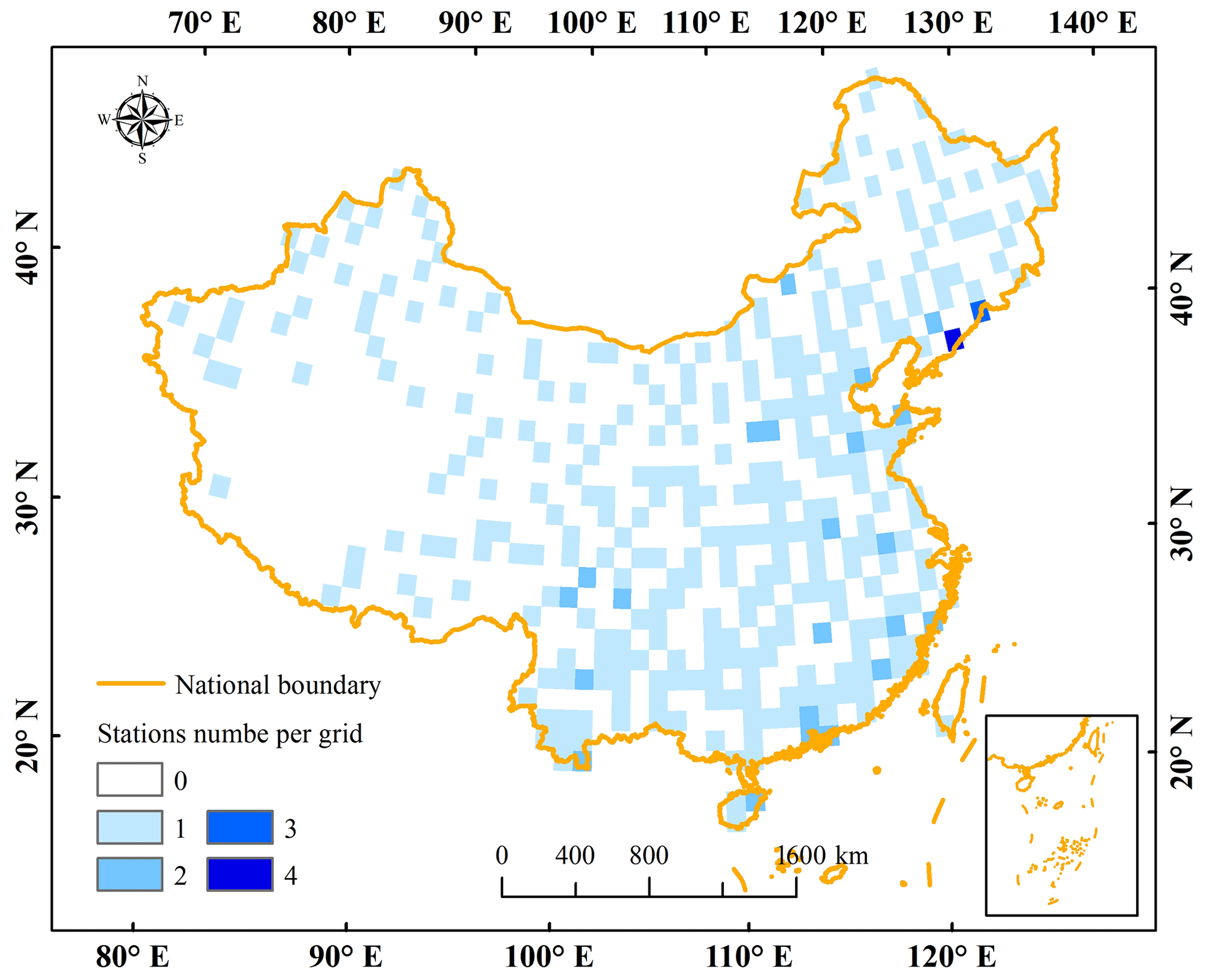
China, between 73–135∘ E and 15–53∘ N, is selected as the study area, which is located in eastern Asia and west of the Pacific Ocean with a land area of 9.6 million km2 (Fig. 1). The elevation of China gradually increases from southeast to northwest, resulting in a complex topography including mountains, plateaus, hills, basins, and plains. China has a diverse climate, including temperate monsoon climate, subtropical monsoon climate, tropical monsoon climate, temperate continental climate, and plateau mountain climate. The Tibetan Plateau is dominated by the plateau mountain climate with a low temperature, strong radiation, abundant sunshine, and little precipitation. However, the southern region has a subtropical monsoon climate characterized by warm winters, hot summers, and abundant rainfall. Annual precipitation over China has high spatial variability, varying between 50 and 2000 mm from west to east. Moreover, the distribution of precipitation amounts and events throughout the year is also extremely uneven. Much more precipitation (70 %–80 %) occurs during the warm season (May to October) than during the cold season (November to April), which is the primary factor for this study to conduct model training according to different seasons. In addition, China is mainly divided into nine river basins, from east to south, including the Continental basin (CB), Songliao River basin (SLRB), Yellow River basin (YERB), Haihe River basin (HARB), Southwest basin (SWB), Yangtze River basin (YARB), Huai He River basin (HURB), Southeast basin (SEB), and Pearl River basin (PRB) (Fig. 1). The runoff of most basins comes mainly from precipitation, while CB is mainly from snow and glacier meltwater.

Figure 1The topography of China and distribution of rain gauges.
2.2 Materials
2.2.1 Rain gauge observations
A relatively dense network of 2372 rain gauges over mainland China from 2000 to 2017 is collected in this study, provided by the China Meteorological Administration (CMA). The daily precipitation data have undergone strict quality control by CMA. These quality control processes include removing extreme values, internal consistency checks, and spatial consistency checks (Shen et al., 2010). Therefore, gauges can be used after simple processing, such as converting units. It should be noted that there is a temporal mismatch (12 h) between daily gauge-based precipitation (Beijing time from 20:00 to 20:00, UTC+08:00) and MSPs (from 00:00 to 24:00 UTC). Considering that not all products have a sub-daily-scale temporal resolution, we recalculate daily observations using sub-daily precipitation (i.e., 08:00 to 20:00 and 20:00 to 08:00) to be consistent with MSPs. Gauges are mainly distributed in eastern China but sparsely located in western China, especially in the hinterland of the Qinghai–Tibet Plateau (TP) (as shown in Fig. 1). The gauge density used in this study is higher than in some previous studies (Wu et al., 2020; Yin et al., 2021; Zhang et al., 2021). The average control area for a single gauge is approximately 4000 km2 (9.6×10⁶ km). Nevertheless, it is far from meeting the requirement of the World Climate Organization that the control area should be about 600 km2 for plains and even smaller for mountain regions (WMO, 2008).
2.2.2 MSPs
Six continuously updated products are selected for integration, including a reanalysis product and five satellite precipitation products retrieved from multiple sensors. Limited by the availability of MSPs, the period of this study is from June 2000 to December 2017 (hereafter: 2000–2017). Specific information about MSPs is summarized in Table 1.
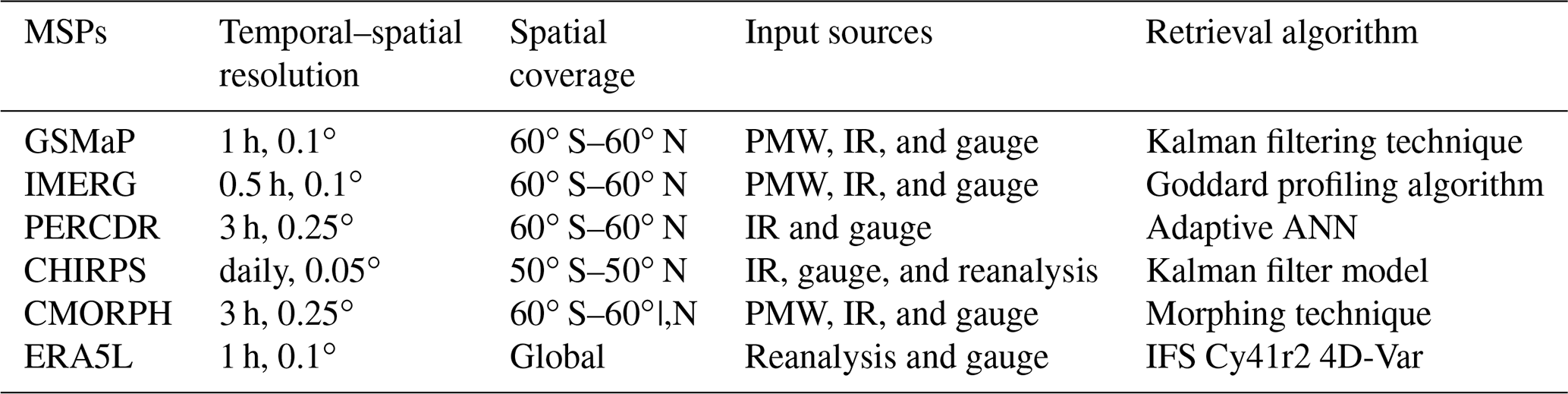
IMERG is the level 3 product of the Global Precipitation Measurement (GPM) algorithm. The IMERG algorithm incorporates the multi-source information from the GPM microwave imager, Visible and Infrared Radiometer (VIRS), and space-borne Ku/Ka-band dual-frequency radar. IMERG provides three types of products, including Early, Late, and Final Run products, which are retrieved around 4 h, 12 h, and 4 months, respectively, after satellite monitoring. The IMERG Final Run product outperforms the Early and Late products because it combines the Global Precipitation Climatology Centre (GPCC) gauge observations. The latest version 6 Final Run product is therefore chosen in this study. Moreover, the Global Satellite Mapping of Precipitation (GSMaP) GSMaP_Gauge applied in this study incorporates Climate Prediction Center (CPC) gauge data analysis (Kubota et al., 2007), which is more accurate than other GSMaP products such as GSMaP near real-time (NRT).
PERSIANN-Climate Data Record (PERCDR) has a long record from 1983 to the present. The PERSIANN algorithm is mainly based on Gridded Satellite (GridSat-BI) IR data and National Centers for Environmental Prediction (NCEP) Stage IV radar data (Ashouri et al., 2015), which does not fuse microwave information. The reliability of PERCDR is improved by using GPCC for calibration. The CHIRPS v.2 product is also used in this study. It has higher spatial resolution than other MSPs, integrating satellite imagery, global climatology, and gauge observations. In addition, the Climate Prediction Center Morphing Technique (CMORPH) version 1 dataset (Joyce et al., 2004) covers products from three categories: CMORPH RAW, CMORPH bias-corrected (CRT), and CMORPH gauge blended datasets (BLD). CMORPH CRT is selected in this study due to its superior quality.
ERA5-Land (herein ERA5L) is an enhanced land atmospheric reanalysis dataset of the fifth-generation ERA5 produced by ECMWF. It provides various land surface variables for more than 70 years with continuous updates. ERA5L describes the evolution of the water and energy cycles on the land in a consistent manner (Hersbach et al., 2020). ERA5L adopts cycle 41r2 of ECMWF's Integrated Forecast System (IFS). Compared with ERA5 and the older ERA-Interim, ERA5L employed a better 4-dimensional variational (4D-var) assimilation technique, with an enhanced horizontal resolution (9 km) and higher spatial resolution (0.1∘). As one of the art-of-the-art reanalysis data, ERA5L has been widely used in many fields (Xin et al., 2021; Xu et al., 2022).
The information sources employed in MSPs show significant differences, especially in terms of whether microwave signals are incorporated or not (Table 1). Moreover, various algorithms are adopted to retrieve precipitation in different MSPs. For instance, the Kalman filtering technique is employed for GSMaP, the Goddard profiling algorithm 2014 is used for IMERG, and the morphing technique is applied for CMORPH (Table 1). Each algorithm and signal source has its pros and cons, and it is necessary to combine them to maximize their advantages. Although several products already combine gauge observation data (e.g., GPCC and CPC) to reduce bias, only a few gauges within China are used. Despite the relatively high gauge density used in this study, this has little impact on the independence of gauges and the reliability of results (Shen et al., 2013). The number and location of gauges used in GPCC over China is shown in Appendix A.
2.2.3 Environment variables
The environment variables used in this study include DEM, longitude, latitude, wind speed, relative humidity, soil moisture, cloud cover, and air temperature.
DEM is downloaded from the Shuttle Radar Topographic Mission (SRTM) with a resolution of 90 m. Wind speed, relative humidity, soil moisture, and air temperature are obtained from the NASA Global Land Data Assimilation System Noah Land Surface Model (GLDAS_NOAH), with 3 h and 0.25∘ resolutions (Rodell et al., 2004). Cloud cover is collected from ERA5 because it is not included in GLDAS_NOAH, with hourly and 0.25∘ resolutions. Although normalized differential vegetation index (NDVI) is often used as a critical auxiliary variable to predict precipitation, it is susceptible to soil type and human activities. NDVI is more suitable for monthly or annual applications due to its temporal resolution (Ghorbanpour et al., 2021; Shen and Yong, 2021; Tan et al., 2021). Inversely, the response of air temperature and soil moisture to daily precipitation is better than NDVI, especially in the desert and bare land (Bhuiyan et al., 2018). In addition, the interactions between cloud properties and precipitation are equally important (Sharifi et al., 2019).
3.1 Data preprocessing
In this study, the period of model training and precipitation interpolation is from 2000 to 2017 at the daily scale. To maintain the temporal and spatial consistency of the data, all MSPs and environment variables at a sub-daily scale are aggregated to daily data. The spatial resolution of DEM (90 m) and CHIRPS (0.05∘) is upscaled to 0.1∘, while the resolution of the PERCDR, CMORPH, cloud cover, and GLDAS_NOAH is downscaled to 0.1∘ using the bilinear interpolation method. In this study, the gauges are divided into two groups: 70 % of rain gauges (1680) are spatially and randomly selected as training and calibrating samples, and the remaining 30 % (692) as validation samples. Due to the irregular distribution of rain gauges over China, random sampling is carried out for each river basin to ensure the spatial representativeness of the validation gauges.
Inspired by previous research (Baez-Villanueva et al., 2020; Zhang et al., 2021), we consider a covariate describing spatial autocorrelation between rain gauges in this study. The semivariogram based on ordinary Kriging is adopted to calculate spatial autocorrelation factors, i.e., Kriging-based prediction (KP). Compared with other predict models, such as inverse distance interpolation (IDW), the Kriging-based semivariogram considers not only the spatial relationship between predicted and neighboring known points but also the statistical autocorrelation between known points. The ordinary Kriging assumes the model as follows:
where z*(x0) is the predicted value of the unknown x0 point. z(xi) and λi are the known value of neighboring rain gauge xi and its weight. Unbiasedness and minimum estimation variance are the conditions for choosing weights. The weight depends on the distance between the known points, the predicted position, and the overall spatial arrangement based on the known points. Spatial autocorrelation must be quantified before spatial arrangement can be applied in weights. The calculation processes of KP are as follows:
-
Calculate the distance and semivariogram between known points,
where γ(h) is the semivariogram of xi and xj, h is the distance, z is the value of known of points.
-
A theoretical model is used to fit semivariogram and distances. The nugget, sill, and range can be obtained according to the fitted semivariogram. The commonly used semivariogram models are spherical, exponential, Gaussian, and linear models. Compared with the prediction performance of KP by different models, the spherical model with better performance is selected in this study. For more information on comparison results, please refer to Appendix B. The spherical model is as follows:
where γ(h) is semivariogram, h is the distance, C0, C, and a is the nugget, sill, and range, respectively.
-
Calculate the semivariogram between the unknown point and known points, and form a matrix to solve the weights:
where μ is Lagrange parameter.
-
Predict the value of the unknown point using Eq. (1) according to the weights obtained from Eq. (4).
3.2 A two-step merging strategy
The specific process of the two-step merging strategy is illustrated in Fig. 2. The RF, GBDT, and XGBoost are chosen to incorporate six MSPs (GSMaP, IMERG, PERCDR, CMORPH, CHIRPS, and ERA5L) and rain gauges. Although the RF method has been extensively employed in most previous studies, few studies compared it with GBDT and XGBoost models in precipitation merging. The environment variables, including soil moisture, cloud cover, relative humidity, air temperature, DEM, longitude, latitude, and spatial autocorrelation (KP), are selected as auxiliary variables (i.e., covariate) of the merging of step 1 and step 2. The values of multiple covariables and MSPs extracted according to gauge locations are taken as independent variables, while gauge observations are taken as the dependent variable. Furthermore, according to the annual distribution characteristics of precipitation, we group all input datasets into two seasons, warm season (May and October) and cold season (November to April), and models are trained independently in each season.
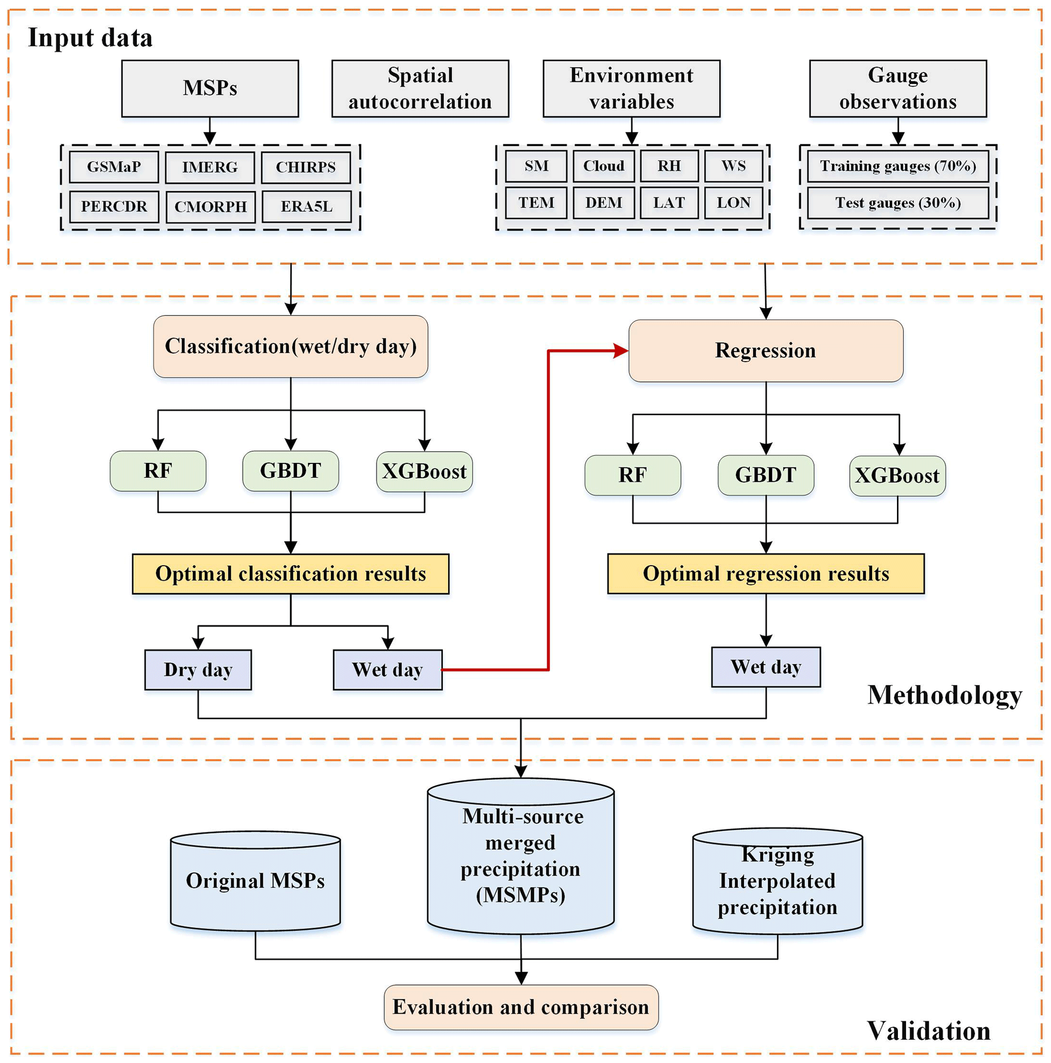
Figure 2Flowchart of the merging strategy used in this study (LAT is latitude, LON is longitude, RH is relative humidity, SM is soil moisture, TEM is temperature, and WS is wind speed).
The two-step merging strategy explored in this study can be generally described in two stages (Fig. 2) as follows:
-
Precipitation classification. The biases of precipitation products mainly come from overestimating/underestimating the amounts of hit events and failing to correctly distinguish precipitation occurrence, including false alarm and missed events (Lei et al., 2022). Therefore, the first step aims to classify precipitation in order to reduce the missed events and false alarm bias. The gauge observations are distinguished into wet/dry days according to the 0.1 mm d−1 threshold value (Lei et al., 2021; Yu et al., 2020; Jiang et al., 2021) and used as the benchmark for classification. The wet day is set as 1 and the dry day is set as 0. The feature values of MSPs and covariables corresponding to each grid are applied to construct XGBoost, GBDT, and RF classification models. The model determines whether a day in the grid is a wet day or a dry day according to the classification probability. Hence, the classification result contains only wet and dry days (0, 1) of each grid and does not involve precipitation intensity. In addition, the model is constructed in warm and cold seasons using divided independent datasets, which leads to six classification models (i.e., two seasons with three models).
-
Precipitation regression. Precipitation regression focuses on improving the precipitation intensity of hit events. The MSPs and covariables values corresponding to the wet day of gauge observations are extracted, which are used to construct and train XGBoost, GBDT, and RF regression models. Similarly, six regression models are trained. The trained regression models are then applied to predict the precipitation amounts of wet days (value equals 1) classified in step (1), while dry days remain 0. The final multi-source merged precipitation products (MSMPs) are obtained by predicted in each grid and day prediction. MSMPs in the whole period are derived from the combination of cold and warm seasons, which are termed “PXGB2”, “PGBDT2”, and “PRF2”, respectively.
To highlight the superiority of the two-step merging strategy, we compare it with single ML regression, multiple linear regression (MLR), and gauge-based Kriging interpolation methods. Moreover, the best-performing algorithm is selected by intercomparing the three ML models in the two-step merging strategy. The detailed merging algorithms are introduced in Sects. 3.2.1–3.2.4.
3.2.1 RF
The RF model was proposed by Breiman (2001) and is widely applied to deal with regression, classification, and other tasks (Rodriguez-Galiano et al., 2012; Nguyen et al., 2021). The general structure of RF is shown in Fig. 3. RF is an ensemble learning algorithm composed of multiple decision trees and generally outperforms a single tree. For regression problems, the model returns predictions by averaging all individual decision trees. For classification problems, each tree in the forest is judged and classified separately, and the output of RF is the class of a majority vote on classification trees (Ho, 1998).
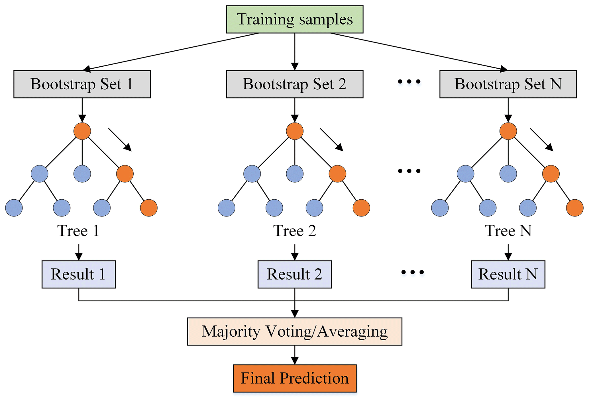
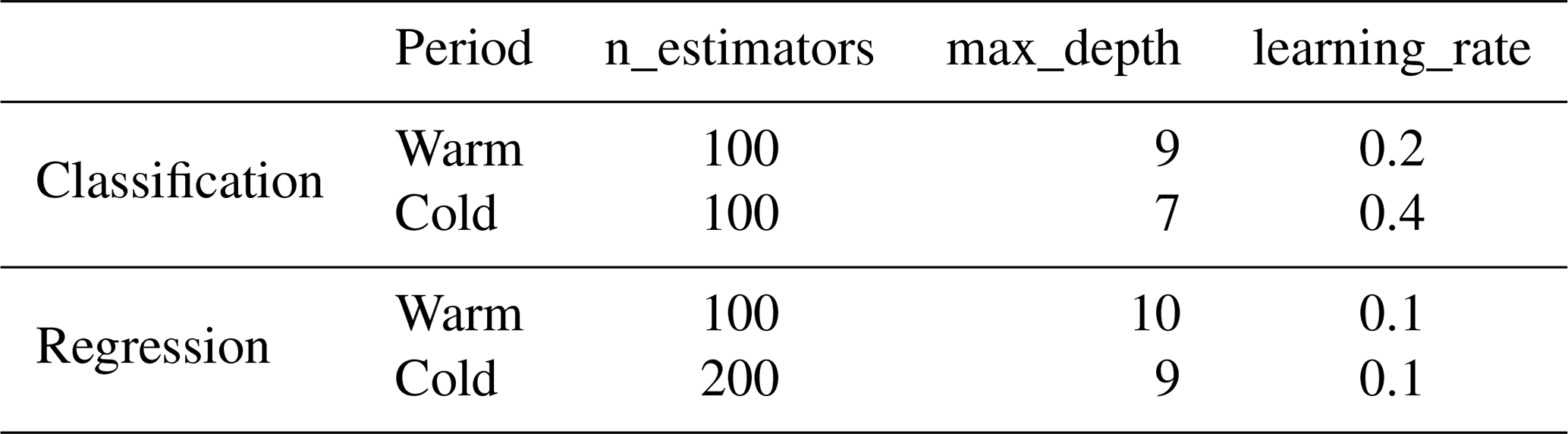
The bootstrap aggregation (i.e., bagging) technique is applied by the RF training algorithm for tree learners, which is designed to improve the accuracy and stability of ML algorithms in classification and regression processes. The bagging algorithm utilizes the out-of-bag (OOB) error to measure the prediction error of RF. It creates two independent datasets. One dataset, the bootstrap sample (approximately two thirds of all samples), is selected as “in-the-bag” data through sampling and replacement, while the remaining OOB dataset (one-third) that is not selected during the sampling process is used to calculate the model's OOB error (Breiman, 2001). The advantages of RF can be mainly summarized in four points: (1) processing high-dimensional data (a mass of features) without dimensionality reduction and feature selection; (2) measuring the importance of features and how they interact with each other; (3) avoiding overfitting and easy to implement; and (4) balancing errors for asymmetric datasets, which is critical in the cold season when wet and dry days are unevenly distributed. In addition, several important parameters in RF are the number of decision trees (n_estimators), the maximum depth of each decision tree (max_depth), and the minimum number of samples required to split an internal node (min_samples_split). A trial-and-error procedure is used to optimize model parameters due to the large sample size used in this study (approximately 14 million pieces of data) and the limitation of computing resources. The optimal parameters of model training during the warm season and cold season are displayed in Table C1 in the Appendix.
3.2.2 GBDT
The GBDT is an iterative decision tree model created by Breiman (1997) and subsequently developed by Friedman (2002), which is also called the “multiple additive regression tree” (MART) (shown in Fig. 4). The additive algorithm is utilized for classification or regression to continuously reduce residuals generated in the training process. GBDT uses the forward distribution algorithm and selects the classification and regression tree (CART) learner as a weak base learner. GBDT generates numerous weak learners through multiple iterations, and each learner is trained based on the residual of the previous learner. It finally integrates the multiple weak learners into a single strong learner by weighting the summation of each tree.
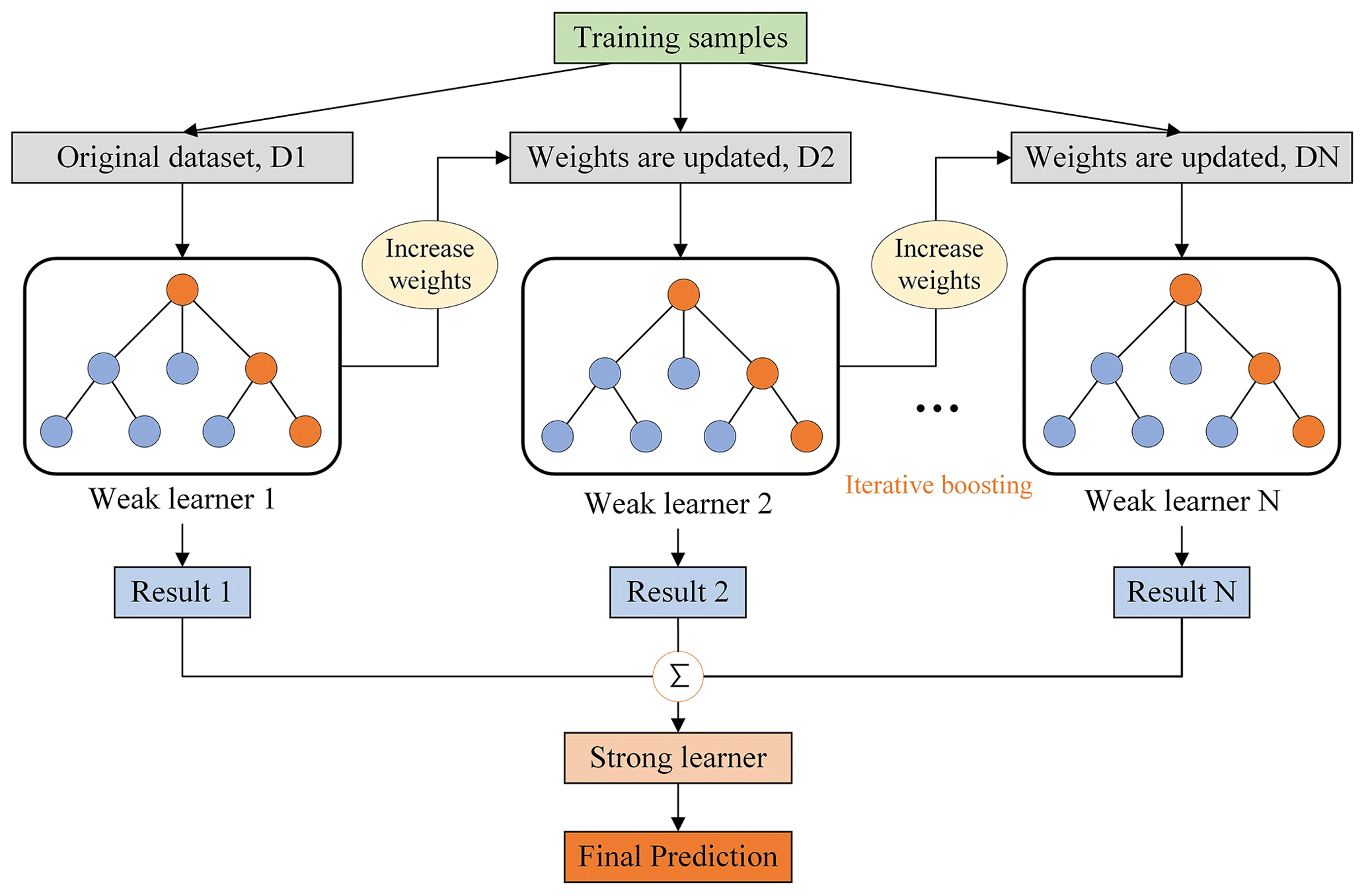
The main difference between RF and GBDT is that RF can be trained in parallel to reduce variances, while GBDT reduces the biases by fitting the residual of former trees. Due to the strong connection between weak learners, GBDT is difficult to be paralleled. Generally speaking, GBDT has superior generalization ability and robustness, which is less affected by training sample size and can deal with various data flexibly, including outliers and irrelevant features. Moreover, the prediction accuracy of GBDT is high in the case of relatively little parameter adjustment time. The main parameters of GBDT include the number of boosting stages to be performed (n_estimators), the learning rate that shrinks the contribution of each tree by learning_rate (learning_rate), and the maximum depth of trees (max_depth). The n_estimators and learning rate are highly correlated with the performance of the model. The optimal parameters are shown in Table C2.
3.2.3 XGBoost
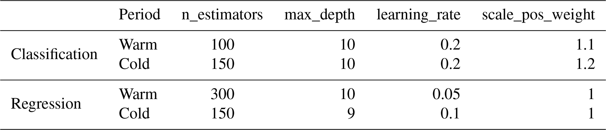
The XGBoost model was proposed by Chen and Guestrin (2016) based on the structure of GBDT. XGBoost also combines multiple weak learners into a strong one, and the base learner in XGBoost can be either CART or linear classifier. XGBoost possesses the strength of GBDT and has several additional improvements: First, GBDT only uses the first-order derivative information in optimization, while XGBoost performs second-order Taylor expansion on the cost function to obtain the first-order and second-order derivatives, thus acquiring more accurate loss functions. Second, XGBoost introduces a regularization term into the cost function to effectively control the complexity of the model. From the perspective of bias–variance tradeoff, it reduces the variance of the model, making the learned model more straightforward and preventing overfitting. Third, XGBoost allows users to define custom optimization goals and evaluation criteria, increasing its flexibility. Moreover, XGBoost implements parallel processing when selecting the best split node for enumeration, substantially improving the computational efficiency compared with gradient boosting machine (GBM). The critical parameters of XGBoost are n_estimators, learning rate, max_depth, and scale_pos_weight. The default value of scale_pos_weight is 1, indicating the positive and negative samples are in equilibrium. This is not applicable for precipitation classification in the cold season. More attention should be paid to scale_pos_weight when model training. The optimal parameters are shown in Table C3.
3.2.4 MLR
The MLR is the first type of regression algorithm used extensively in many fields, assuming a stable linear relationship between a dependent variable and multiple independent variables. Compared with nonlinear relationships, the MLR is easier to fit and each explanatory variable's statistical property is more intuitive. MLR is usually fitted using the ordinary least square method to minimize the sum of squares of residuals predicted by the model and observed by the sample. The overall model for MLR is
where n is the number of explanatory variables, Y is the dependent variable predicted by X1, X2 …, Xn. β0 is the intercept, and β1, β2, … βi are regression coefficients.
3.3 Performance evaluation and comparison
In this study, the performance of all products is evaluated using 692 randomly selected independent gauges from 2000 to 2017. The evaluation metrics mainly involve categorical and statistical metrics. The categorical metrics focus on analyzing the ability of products to capture precipitation events, including the probability of detection (POD), false alarm ratio (FAR), critical success index (CSI), precision (precision), frequency bias (FB), Heidke Skill Score (HSS), and classification accuracy (accuracy). The POD, also called “hit bias”, represents the probability of precipitation events correctly detected. FAR and “precision” describe the ratio of falsely and correctly detected events among total detected precipitation events, respectively. The sum of FAR and precision is 1. The CSI incorporates POD and FAR, which demonstrates the overall ability of precipitation detection. The FB is the ratio of POD and FAR; it shows the balanced ability of products in detecting precipitation events. FB < 1 indicates that precipitation events are underestimated, and FB > 1 indicates that they are overestimated. The FB equals 1, meaning that the number of missed events equals false alarm events. HSS compares the predicted performance with random chance. The negative HSS shows random chance is better than the model predicted. The range of HSS is −∞ to 1, the perfect value is 1.
“Accuracy” shows the proportion of total days that are correctly classified as wet and dry days. One point that needs to be emphasized is that this study takes accuracy as the evaluation metric to describe the accuracy of ML classification models (RF, GBDT, and XGBoost) in training processes, thereby determining the optimal parameters of the model.
where H is the total number of precipitation events simultaneously observed and predicted, M is the total number of precipitation events observed but not predicted, F is the total number of precipitation events predicted but not detected, N is the total number of no-precipitation events. The optimal value of POD, precision, CSI, accuracy, and FB is 1, while FAR is 0.
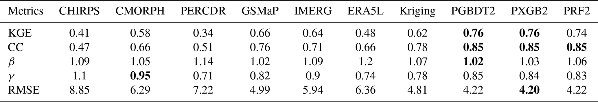
The statistical metrics are used to evaluate the error in estimating precipitation intensity, including root mean square error (RMSE), the modified Kling–Gupta efficiency (KGE) and its components – Pearson correlation coefficient (CC), bias (β), and variability ratio (γ). The CC measures the magnitude of the correlation between the model-predicted and observed values. The RMSE accesses the error between predicted and observed values. The KGE combining the CC, β, and γ reflects the overall goodness of fit between model-predicted and observed values. β>1 indicates precipitation amount is overestimated and vice versa. The formulas for these metrics are expressed as follows:
where Po and Pm are the value of gauge observed and predicted precipitation, respectively. N is the total number of samples; μm and μo are the mean value of gauge observed and predicted precipitation, respectively; and SDo and SDm are the standard deviation of gauge observed and predicted precipitation, respectively. The optimal value for CC, KGE, β, γ is 1, while for MAE and RMSE it is 0.
4.1 Evaluation of the precipitation detection ability of MSMPs
The classification accuracy of different ML models for wet/dry days is shown in Table 2. The general performances are considerable. The accuracy for the three models is higher than 91 % in the whole period, which is 91.8 %, 91.7 %, and 91.8 % for RF, GBDT, and XGBoost, respectively. The accuracy in the cold season is better than that in the warm season. There is no significant difference among the three classification algorithms. The main reason is that the input variables used in this study are sufficient in variety and quantity.
Table 2The classification accuracy of wet/dry days during the warm season and cold season.
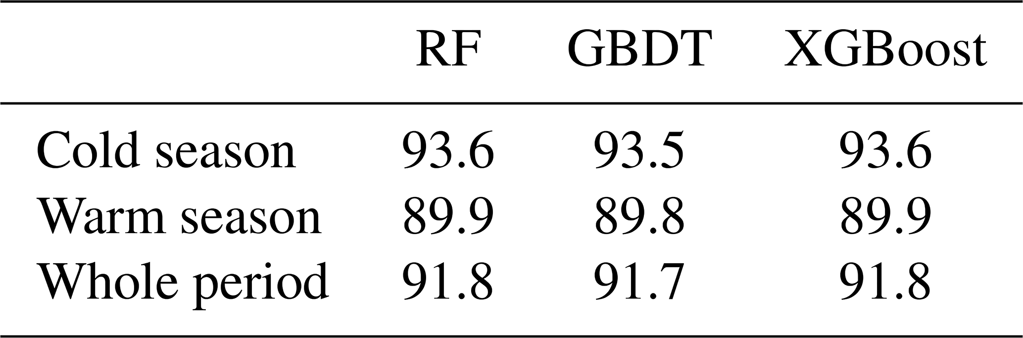
Table 3The average value of categorical metrics of multiple products compared with gauge observations during the whole period.
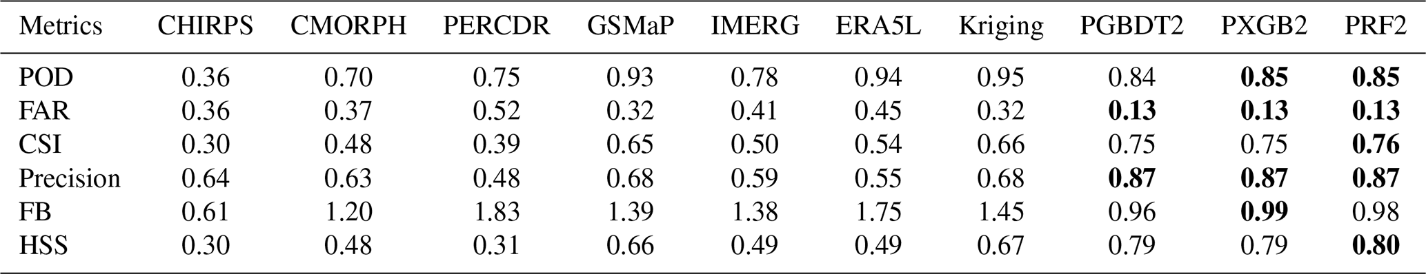
Note: the values in bold are the best performing of each metric.
To evaluate the efficiency of the proposed strategy in precipitation detection ability, the MSMPs (PGBDT2, PXGB2, and PRF2), gauge-based Kriging interpolated (Kriging), and original precipitation products (MSPs) are assessed and compared based on independent gauge observations. The six categorical metrics (POD, FAR, CSI, precision, FB, and HSS) are shown in Fig. 5 and the average values of all gauges are presented in Table 3. The overall accuracy of three MSMPs substantially outperforms other products. The best values of all metrics (except for POD) are generated in MSMPs. Kriging has the highest POD with a value of 0.95 (Fig. 5a), followed by ERA5L (0.94) and GSMaP (0.93). However, the POD of PGBDT2, PXGB2, and PRF2 is 0.84, 0.85, and 0.85, respectively. The FAR (Fig. 5b) of MSMPs is 0.13, decreased by 59 %–75 % compared with the original MSPs (0.32–0.52). In addition, PRF2 obtains the highest CSI with a value of 0.76, much better than the original MSPs (0.3–0.65) and Kriging (0.66) (Fig. 5c). In terms of precision (Fig. 5d), the MSMPs show an obvious improvement. The precision increases from 0.48–0.68 (MSPs) to 0.87 (MSMPs). For FB (Fig. 5e), MSPs and Kriging deviate from 1, and PERCDR has the worst value (1.83). Although ERA5L achieves a high POD, its FB is 1.75, indicating ERA5L has seriously overestimated wet days and misclassified many precipitation events. Fortunately, MSMPs strike a good balance between hit and false alarm rates. The FB of MSMPs is closer to 1, which is 0.96 for PGBDT2, 0.99 for PXGB2, and 0.98 for PRF2. In terms of HSS (Fig. 5f), except for Kriging (0.67) and GSMaP (0.66), the HSS of MSPs is lower than 0.5 (0.3–0.49). By contrast, the MSMPs (0.79–0.8) improve by 20 %–163 %.
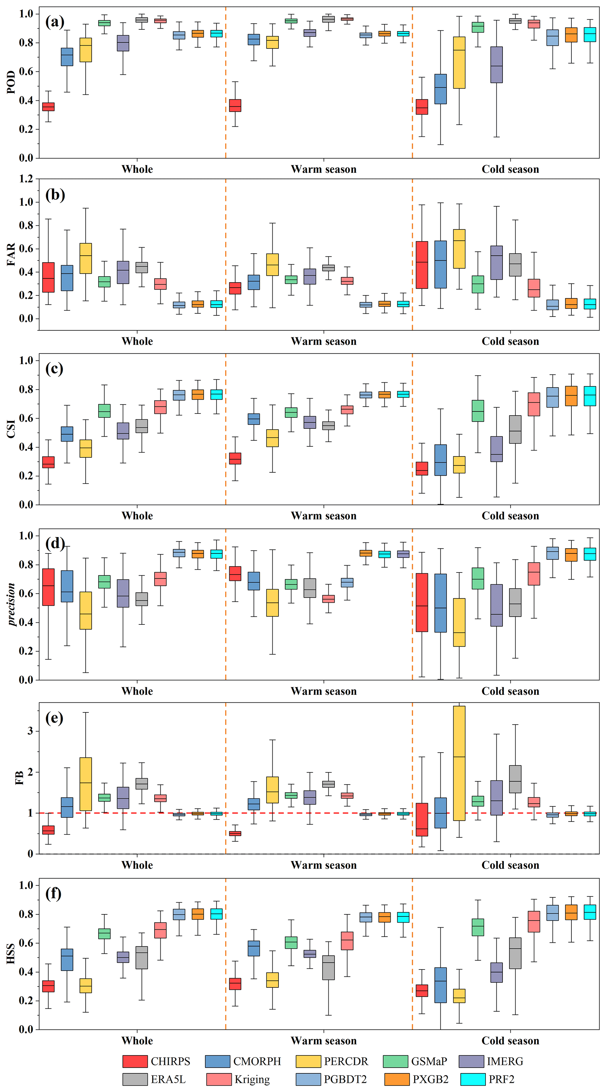
Figure 5Boxplots of six categorical metrics (POD (a), FAR (b), CSI (c), precision (d), FB (e), and HSS (f)) for 10 products, including six MSPs, one gauge-based interpolated data, and three ML-based merged data.
The general performance of most MSPs (e.g., CMORPH, PERCDR, and IMERG) in the warm season is better than that in the cold season (Fig. 5). However, the difference in the performance of MSMPs between warm and cold seasons is smaller than that of MSPs, demonstrating that the ability of MSMPs is more balanced throughout the year. Moreover, the variation in metrics of the original MSPs is considerable in the cold season, particularly FAR and precision. The boxplots of FAR (Fig. 5b) and of precision (Fig. 5d) for CHIRPS, CMORPH, and PERCDR have wider ranges, which shows these values have an uneven spatial distribution. By contrast, MSMPs have more concentrated ranges of boxplots in most metrics. These results emphasize the necessity of prioritizing precipitation state recognition in the merging process, which can greatly improve the precipitation capture efficiency of MSPs.
Figure 6 shows the average value of six categorical metrics for 10 products under different precipitation intensities, including no precipitation (<0.1 mm d−1), light precipitation ([0.1, 5)), moderate precipitation ([5, 20)), heavy precipitation ([20, 50)), and violent precipitation (>50 mm d−1). Overall, MSMPs have the best performance regardless of precipitation intensities, followed by Kriging and GSMaP, signifying that ML classification techniques improve the detection capability of all precipitation thresholds, not only for light and moderate precipitation events. The performance of all products for no precipitation is considerably better than other precipitation intensities. For instance, the FAR, CSI, and HSS of MSMPs are 0.07, 0.88, and 0.79–0.8, respectively, in no precipitation. Most MSPs have a poor ability to capture light and moderate precipitation (0.1–20 mm d−1). The CSI of MSPs ranges between 0.07 and 0.43 and HSS is 0.06–0.54, while the HSS of MSMPs varies between 0.58 and 0.6. In addition, the FB fluctuates greatly in light precipitation, with the lowest value of 0.34 for CHIRPS and the largest value of 2.09 for PERCDR (Fig. 6e). The MSMPs show the best FB values of 0.85. The accuracy begins to decrease when precipitation intensity is above 20 mm d−1 (i.e., heavy and violent precipitation). For violent precipitation (>50 mm d−1), the reduction in accuracy of MSMPs and Kriging is relatively small compared with the original MSPs. MSMPs have the highest POD (0.39–0.4), CSI (0.33), and HSS (0.47). However, the FAR and precision show a different trend with better accuracy in violent precipitation than in moderate and heavy precipitation (Fig. 6b and d). In addition, although the POD of ERA5L and Kriging outperform MSMPs for whole events, they are inferior to MSMPs in moderate, heavy, and violent precipitation. Generally, XGBoost and RF models are slightly superior to GBDT when dividing precipitation thresholds (Fig. 6a). Kriging exhibits better performance than most original MSPs. Nevertheless, it is only based on gauge observations and does not combine other climate variables associated with precipitation processes. When MSPs, gauge, and multiple covariates are considered, the MSMPs are more accurate than Kriging.

Figure 6The performance of six categorical metrics (POD (a), FAR (b), CSI (c), precision (d), FB (e), and HSS (f)) of 10 products under various daily precipitation thresholds.
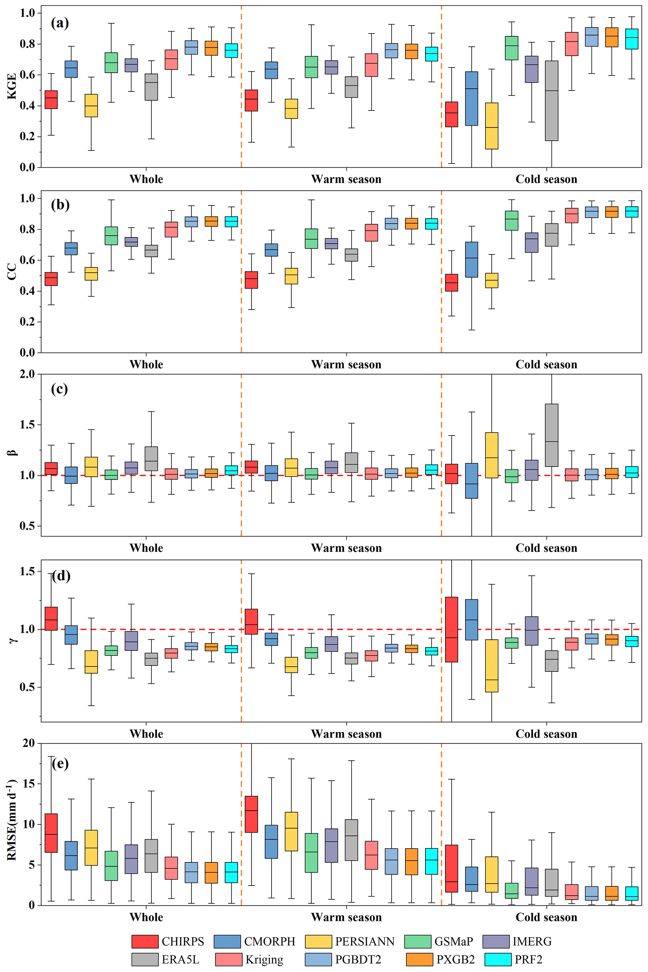
Figure 7Boxplots of five statistical metrics (KGE (a), CC (b), β (c), γ (d)), RMSE (d)) and for 10 products.
Table 4The average values of statistic metrics of multiple products compared with gauge observations during the whole period (the unit of RMSE is mm d−1).
Note: the values in bold are the best performing of each metric.
4.2 Evaluation of the precipitation amounts of MSMPs
To explore the accuracy of the precipitation amounts of MSMPs, five statistical metrics (RMSE, KGE, and its components CC, β, and γ) are employed to compare original MSPs and Kriging with PGBDT2, PXGB2, and PRF2 based on daily observations. According to the comparison results (Fig. 7, Table 4), the MSMPs perform better than all original MSPs. The KGE of MSPs is improved by 15 %–85 % in the whole period (Fig. 7a). The KGE is 0.74–0.76 for MSMPs, 0.62 for Kriging, and 0.34–0.66 for MSPs. MSMPs have a strong correlation with gauge observations in the warm season (CC: 0.83), cold season (CC: 0.9), and the whole period (CC: 0.85) (Fig. 7b), which is substantially better than MSPs (warm: 0.45–0.75; cold: 0.45–0.83; whole: 0.47–0.76). In addition, β shows that all MSPs and Kriging overestimate precipitation amounts (Fig. 7c). This overestimation is more prominent in the cold season, with values ranging between 5 % and 38 %. By contrast, MSMPs show significant improvements and obtain better results in all seasons. Although GSMaP and CMORPH have better performance than PRF2 during the warm season and the whole period, they suffer from a large magnitude of overestimation (Kriging: 6 %; CMORPH: 13 %) in the cold season. In terms of γ, the average variability ratio of CHIRPS, CMORPH, and IMERG is more consistent with 1 compared with MSMPs (Fig. 7d). However, they show more discreteness, particularly for CHIRPS. In comparison, the distribution of MSMPs values is more compact. The results indicate that MSMPs can merge the complementary advantages of original data and reduce errors to a large extent, especially in the cold season. For RMSE (Fig. 7e), the values in the warm season are higher than those in the cold season. This is because precipitation is mainly concentrated in the warm season, and higher precipitation amounts often lead to larger RMSE. The RMSE for MSMPs decreases by 16 %–52 % compared with the original MSPs (4.99–8.85 mm d−1). Among MSMPs, PXGB2 exhibits the smallest RMSE with a value of 4.2 mm d−1.
Figure 8 illustrates the spatial distribution of RMSE and KGE for GSMaP, Kriging, and PXGB2 in the whole period. The reason for showing only these three products is that they perform better among original products and MSMPs. The spatial comparison among them is more representative and brief. The RMSE gradually increases from north to south, which is consistent with the precipitation change pattern (Fig. 8a). The RMSE for the PXGB2 in south China has better performance than Kriging and GSMaP. For PXGB2, approximately 48 % of the gauges have an RMSE less than 4 mm d−1. The percentage of gauges with an RMSE higher than 8 mm d−1 is 14 % for GSMaP, 8 % for Kriging, and 4 % for PXGB2. In addition, the spatial distribution of KGE shows that the low values are mainly gathered in the northwest (Fig. 8d–f). For PXGB2, about 36 % of the gauges have a KGE higher than 0.8, compared with only 15 % for GSMaP and 30 % for Kriging. The PXGB2 improves KGE performance over the northwest region and narrows the gap between the southeast and northwest regions. These results indicate that the two-step merging approach could mitigate the spatial variability of products and is less susceptible to topography.
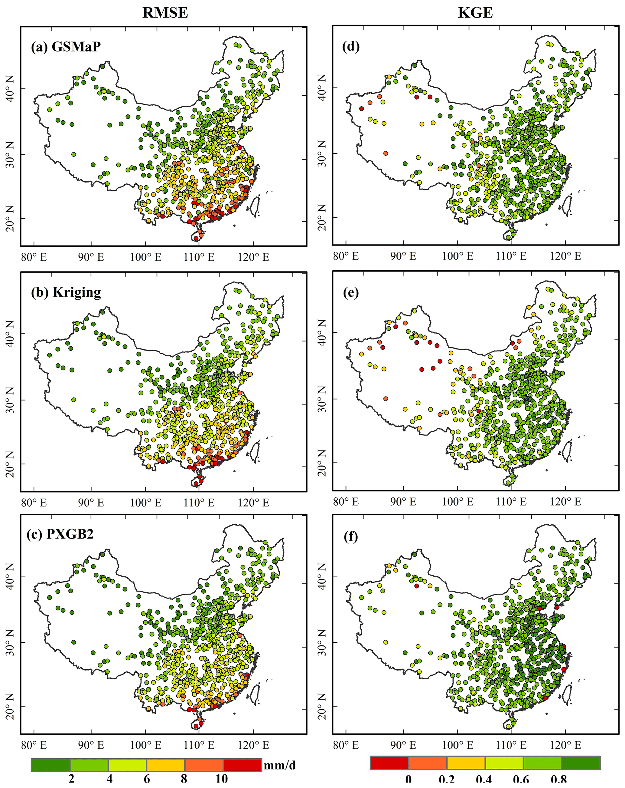
Figure 8Spatial distribution of RMSE (a–c) and KGE (d–f) for GSMaP (a, d), Kriging (b, e), and PXGB2 (c, f) in the whole period from 2000 to 2017 using independent rain gauges over mainland China.
4.3 Variable importance in ML models
Variable importance can quantitatively explain the contribution of variables to improving model accuracy and can identify crucial input variables. The permutation feature importance is utilized to calculate variable importance values of models. The basic idea of this method is to randomly shuffle the order of a specific variable while keeping other variables unchanged and compute the difference in accuracy (the evaluation metric is accuracy for the classification model, mean squared error for the regression model) with the original model. As shown in Fig. 9, the importance of variables for GBDT, XGBoost, and RF and their ranks are different, which is related to the inherent structure of each model. This phenomenon also exists between classification and regression models. Nonetheless, KP is always the most important variable in each model, proving that the Kriging-based predictor considering the spatial autocorrelation between rain gauges is helpful in improving model efficiency. For all models, the top three variables in importance are KP, GSMaP, and IMERG. The CMORPH, PERCDR, ERA5L, and temperature are considered next in significance. The importance of ERA5L and temperature in XGBoost and RF classification models is more obvious than that in regression models. Additionally, longitude, latitude, DEM, cloud cover, and relative humidity exhibit a relatively low influence on precipitation merging. The impacts of CHIRPS, soil moisture, and wind speed on prediction results are negligible. However, this does not mean that these predictors are not important for precipitation in whole regions. The slight importance of the latter variables may be affected by data quality and the correlation degree with precipitation. For example, CHIRPS is the worst performing product among original MSPs. Overall, it is necessary to employ multiple covariables in classification and regression models since complex precipitation processes cannot be thoroughly described by a single variable.

Figure 9Permutation feature importance of three (GBDT, XGBoost, and RF) classification models (a–c) and three regression model (d–f) in the warm season (LAT is latitude, LON is longitude, RH is relative humidity, SM is soil moisture, TEM is temperature, and WS is wind speed).
5.1 Comparison of the different merging strategies
From the aspect of merging processes, different models and training samples could affect the accuracy of the integrated dataset. Therefore, three additional merging scenarios are considered for quantitative comparison with the proposed strategy to highlight the impact of sample division and algorithm selection on fusion results. Figure 10 gives a brief overview of four scenarios and their corresponding merged precipitation products. Scenario 1 is the method adopted in this study; scenario 2 separately trains the model in each season based on four regression models (GBDT, XGBoost, RF, and MLR), and the corresponding results are PGBDT_R, PXGB_R, PRF_R, and PMLR; scenario 3 applies classification and regression models during the entire period, and the results are PGBDT_E, PXGB_E, and PRF_E; while scenario 4 solely employs four regression models during the entire period, and the results are PGBDT_ER, PXGB_ER, PRF_ER, and PMLR_ER.
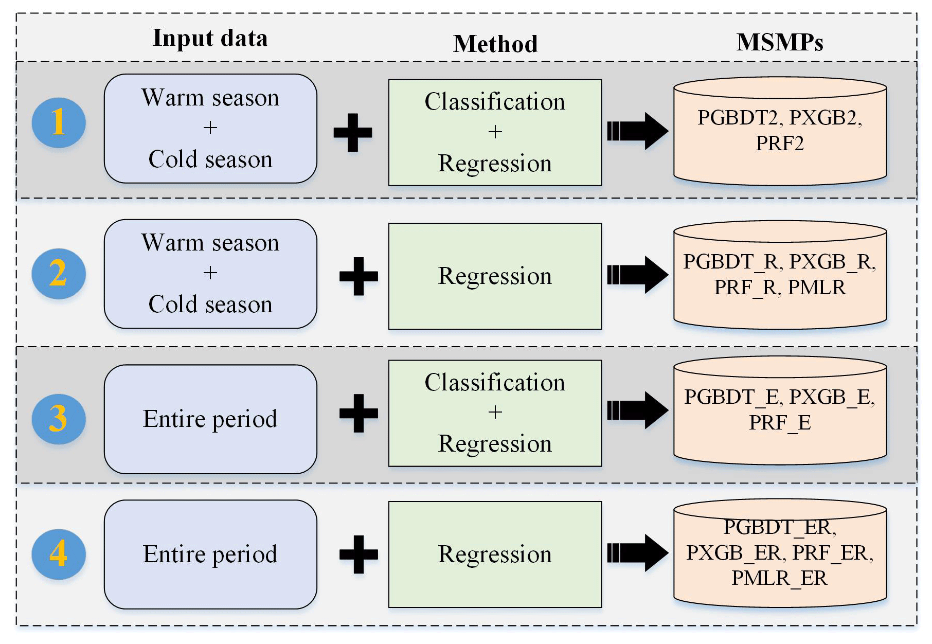
Figure 11 shows the evaluation results (CC, CSI, KGE, FB, and HSS) of four scenarios between 14 MSMPs with independent gauge observations. The performance of scenario 1 is apparently better than the other scenarios. For scenario 2, although the statistical metrics (CC and KGE) are only slightly worse than scenario 1, the categorical metrics (CSI, FB, and HSS) are considerably weakened. In the whole period (Fig. 11a), the HSS is between 0.64 and 0.68 for scenario 2, much lower than 0.79–0.8 for scenario 1. Moreover, the FB of scenario 2 is larger than 1.38 (Fig. 11a), indicating that the number of precipitation events is overestimated. A similar phenomenon also occurs in warm and cold seasons (Fig. 11b and c). Furthermore, the MLR performs worse than the three ML models. The results of scenario 2 demonstrate that only relying on regression models to merge precipitation can describe precipitation intensity but not capture precipitation occurrence well. In scenario 3, the overall performance is superior to scenario 2 but inferior to scenario 1. The CSI (Fig. 11c) for scenario 1 and scenario 3 ranges from 0.73 to 0.74 and from 0.70 to 0.72, respectively. Scenario 3 suggests that merging precipitation in different seasons could balance the performance differences within a year. Scenario 4 shows the worst performance regardless of season, with poor CSI, FB, and HSS. Especially for the PMLR-ER dataset, its accuracy is even worse than GSMaP and Kriging. This is because with MLR it is difficult to describe the complex relationship between precipitation and other variables. The four scenarios can be ranked by prediction accuracy from best to worst: scenario 1 > scenario 3 > scenario 2 > scenario 4. The approach (i.e., scenario 1) employed in this study is proved to be more accurate than other traditional strategies.
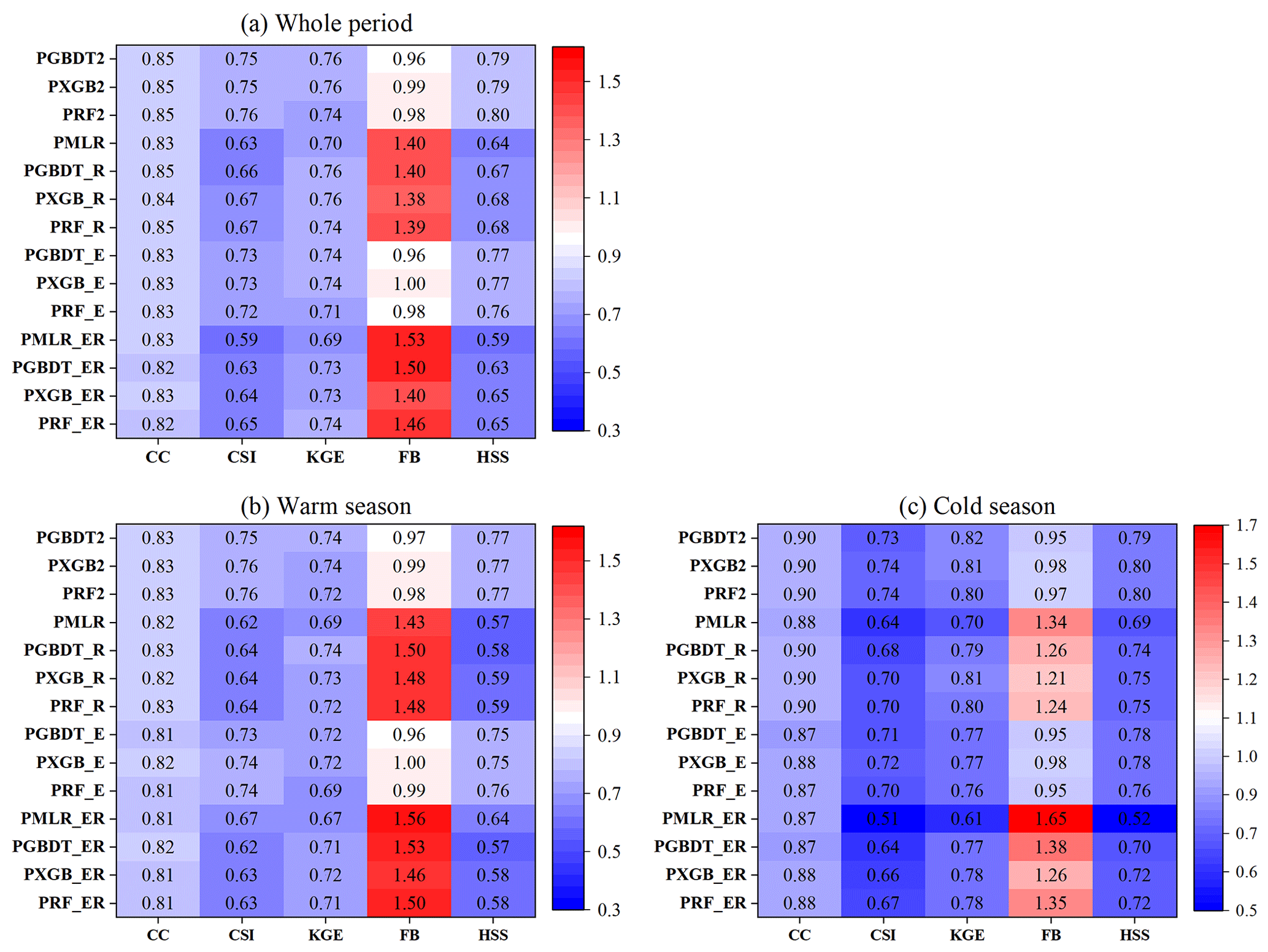
Figure 11Five evaluation metrics (CC, CSI, KGE, FB, and HSS) for different products under four scenarios during the whole period (a), warm season (b), and cold season (c).
5.2 Models efficiency
The GBDT, XGBoost, and RF models show similar improvements in the two-step merging strategy. Nevertheless, different models have their inherent advantages and disadvantages. There is an apparent disproportion between positive and negative samples (wet and dry days) when training the classification model, which directly impacts the model's classification accuracy. In this study, the proportion of positive and negative samples in the cold season is approximately 1:3.2. In terms of this imbalance problem, RF and XGBoost algorithms have built-in parameters for adjusting. However, GBDT requires additional oversampling methods such as the synthetic minority oversampling technique (SMOTE) to be solved, which increases the complexity of model training. Moreover, it can be inferred from the results of Table 3 and Figs. 5 and 11 that the FB of XGBoost outperforms RF in all seasons, indicating XGBoost has better equilibrium ability for disproportional samples. In addition, Fig. 12 displays the computational costs of training for three models under different sample sizes. The result shows that the training time of GBDT and RF is much higher than XGBoost, which is mainly related to the model structure and parallel training. XGBoost parallels the feature granularity rather than the tree granularity. The most time-consuming part of decision tree learning is sorting feature values to determine the optimal split node. XGBoost ranks the values before training and then saves them into a block structure, which is repeatedly used in subsequent iterations. In this way, the training time can be greatly reduced (Chen et al., 2016; Wang et al., 2019). Therefore, considering the complexity, accuracy, and computational costs of the model, XGBoost is an optimal choice for predicting daily precipitation over China.

5.3 The influence of gauge density and spatial resolution
The density of rain gauges can influence the performance of the merged product as well as the gauge-based interpolated product. Gauges with different densities are used to train the model and for interpolation, including 10 %, 30 %, 50 %, and 70 % of total gauges. Figure 13 shows that the higher gauge density leads to a better performance of the merged and interpolated products. However, PXGB2 is less affected by the density compared with Kriging. The decreased magnitude of Kriging accuracy is more significant than that of PXGB2 as the gauge number is reduced. For instance, the deterioration in the KGE is 0.04 for PXGB2 (0.76 to 0.72) but 0.32 for Kriging (0.63 to 0.31), which is also smaller than that reported by Baez-Villanueva et al. (2020) and Zhang et al. (2021). The precipitation capture efficiency of PXGB2 decreases slightly and always shows a better performance. The CSI and HSS of PXGB2 vary from 0.73 to 0.76 and from 0.77 to 0.79, respectively. The FB is relatively stable under different gauge numbers. In addition, even when gauge density is reduced to 10 % (237 gauges, i.e., 40 000 km2 per gauge), PXGB2 also outperforms Kriging at 70 % (1680 gauges) and the best original MSPs (i.e., GSMaP). In comparison, the performance of Kriging is inferior to GSMaP when gauge density is less than 50 %, especially at 10 %, which shows the gauge-based interpolation method is more suitable for high gauge density regions and could lead to considerable uncertainties in low gauge density regions. In general, these results demonstrate that the proposed method is effective and robust, and it is expected to be applied to improve precipitation accuracy in areas with scarce data.
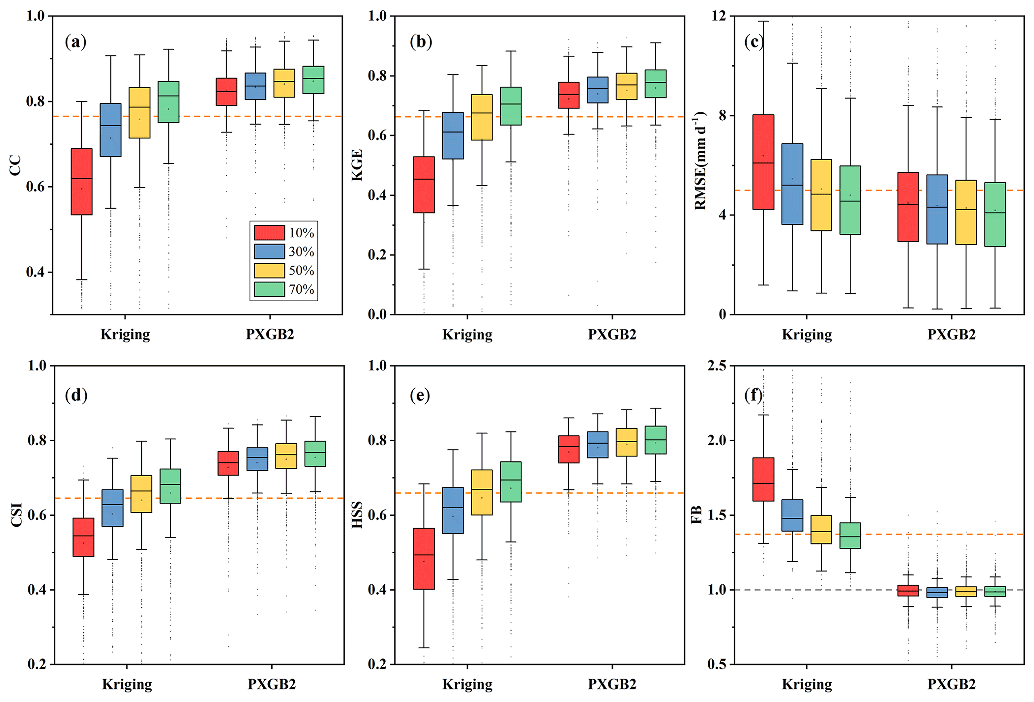
Figure 13Performance of PXGB2 and Kriging products using training dataset with different rain gauge densities (10 %, 30 %, 50 %, 70 %). The dotted orange line in (a)–(f) shows the average of the best original product (GSMaP). The dotted gray line in (f) represents the reference line with a value of 1.
This study uses a simple interpolation method to resample products to keep a consistent spatial resolution and avoid additional uncertainties, as many previous studies have done (Chao et al., 2018; Zhang et al., 2021; Baez-Villanueva et al., 2020; Wu et al., 2020; Wang et al., 2020; Hong et al., 2021). Figure 14 shows the performance of PXGB2 obtained by training models with precipitation products under different spatial resolutions (0.05, 0.1, and 0.25∘). It demonstrates that there are only slight differences between various resolutions during the whole period as well as during warm and cold seasons, which is consistent with the results of a previous study (Baez-Villanueva et al., 2020). Therefore, it can be considered that unifying the spatial resolution of all products to 0.1∘ has a negligible impact on the merging results in this study.

Figure 14The performance ((a) KGE and (b) CSI) of PXGB2 prepared by MSPs with different spatial resolutions (0.05, 0.1, and 0.25∘) during the whole period, warm season, and cold season.
5.4 Comparison with previous studies
The study combines classification and regression models to improve the accuracy of MSPs, which pays special attention to optimizing precipitation detection ability and reducing the error caused by missed events and false alarms. This research has made significant progress based on the achievements of previous studies. In terms of precipitation occurrence, the classification accuracy (91.8 %) is better than the ANN model (86.5 %) applied by Xiao et al. (2022) and the RF model (77.5 %) employed by Pham et al. (2019). The POD of MSMPs is lower than GSMaP and ERA5L, which is similar to the results of Xiao et al. (2022). In addition, Yin et al. (2021) improved the CC of the original product by 11 % and the RMSE by 7 % over China, which is slightly inferior to the improvement in this study (CC and RMSE improved by 12 % and 16 %, respectively). Furthermore, the overall performance of MSMPs is substantially better and could provide more accurate precipitation information for hydrological research. The CC of MSMPs is up to 0.85, much higher than 0.78 reported by Zhang et al. (2021), 0.61 by Yin et al. (2021), and 0.72 by Wu et al. (2020) over China. Although the validation method and period vary in the different studies, their conclusions still have reference value. The better performance found in this study is mainly due to the consideration of precipitation products from multiple sources, environment variables, and relatively higher gauge density. Most importantly, the spatial autocorrelation considered in this study plays an important role in the merging process. Compared with considerations of spatial distance (Baez-Villanueva et al., 2020), geographical coordinates, and spatial correlation (Zhang et al., 2021), it not only can describe spatial autocorrelation between gauges but also between rain gauges and predicted points. In addition, some previous studies based on statistical methods were complex and difficult to reproduce for researchers in other fields (Yang et al., 2017; Ma et al., 2021; Yin et al., 2021). For instance, Yang et al. (2017) combined the MSPs and gauges by bias correction, gauge observation gridding, and data merging. In comparison, the proposed method only relies on ML and does not involve other statistical methods, which is easy to implement and has broad transferability.
5.5 Limitations and uncertainties
Although this proposed merging strategy has achieved outstanding performance, some issues still need to be discussed and further improved in future studies. The gauge observations are taken as the reference in model training and evaluation. However, the strategy suffers from uncertainties induced by diverse climates, complex topography, and measuring instruments (Ma et al., 2015; Lei et al., 2021). These uncertainties are more obvious in the gauges located in regions with snow and glacier coverage and would be propagated to merged precipitation results. Moreover, gauges at high altitudes are sparsely distributed and have strong spatial heterogeneity, making it challenging to describe precipitation distribution accurately. In future studies, the input datasets could be divided into more groups according to different terrains or altitude zones, and precipitation data in high-altitude regions could be corrected by combining topographic factors, snowfall, and glacier mass balance data to mitigate their uncertainties.
This study assumes that the rain gauge represents the areal precipitation pattern in its corresponding grid, but this assumption is not fully satisfied in practical applications, especially in the Tibetan Plateau. This spatial scale mismatch problem between precipitation gridded data and single gauge observations can be alleviated by downscaling coarse products to a finer resolution. Some studies have downscaled all monthly products before merging them with gauge observations (Chen et al., 2018, 2021). However, downscaling daily precipitation is challenging because it is difficult to describe the relationship between precipitation and environment variables (Chen et al., 2021). More effective downscaling algorithms are worth exploring in the future.
Due to the limitations of gauge observations, the benchmark and MSPs used in this study are not near real-time products. The merged products are more suitable for studying hydrometeorological changes in long time series than in the middle or short term. Multi-source precipitation products with near real-time and finer temporal resolution can be continuously merged, such as IMERG Early Run and GSMaP_NRT, to improve the accuracy of precipitation for flood prediction if rain gauges are available. In addition, although the trained model has spatial transferability, there is uncertainty when applied to precipitation prediction outside the training period.
This study proposes a two-step merging strategy including GBDT, XGBoost, and RF classification and regression algorithms to merge MSPs, multiple environment variables, and rain gauges from 2000 to 2017 over China. The performance of three merged products (MSMPs) is validated based on 692 randomly selected independent gauges and compared with original MSP, Kriging, and other traditional merging scenarios (e.g., ML regression and MLR). Several statistical and categorical metrics are employed to quantitatively describe the precipitation detection capability and precipitation uncertainties. The main findings of this study can be summarized as follows:
-
The precipitation capture ability of MSPs has been substantially improved. The MSMPs are better than all original MSPs and Kriging regardless of the precipitation intensity. The CSI for MSPs and Kriging is 0.30–0.65 and 0.66, while MSMPs are increased to 0.75–0.76. The HSS is also improved by 21 %–16 % (0.79–0.8) compared with MSPs (0.30–0.66).
-
The statistical biases of precipitation amounts induced by hit events are obviously alleviated. The improvement of CC, KGE, and RMSE is 12 %–81 %, 15 %–85 %, and 16 %–52 %, respectively. The spatial difference in precipitation accuracy between northwest and southeast China is also narrowed.
-
It is essential to incorporate spatial autocorrelation in the merging strategy. KP is the most important covariable in precipitation merging, followed by GSMaP, IMERG, and ERA5L. The degree of importance for covariables in models also relates to their inherent accuracy.
-
Compared with traditional MLR and ML regression models, the proposed method in this study has superior performance in all aspects. Moreover, the MSMPs predicted by considering annual precipitation characteristic distribution are better than those in the whole period.
-
The higher gauge density used in model training could lead to a better performance of the proposed method. However, this method could also remarkably improve original products even with few gauges.
-
The comprehensive ability of RF and XGBoost is slightly better than GBDT. Considering the computation efficiency, it is recommended to use XGBoost to prepare merged precipitation products.
The two-step merging strategy proposed in this study achieves satisfactory performance over China. It is robust and efficient in such a region characterized by complex terrain, variable climate, and uneven distribution of gauges. Therefore, this method has great referential significance and can also achieve excellent results when applied in other regions and countries.
From the latest GPCC dataset, the number of China's International Exchange Stations used in GPCC has fluctuated between 360 and 370 (in Fig. A1, the number is 362 in July 2015), which has increased in recent years. Before 2017, only about 200 of China's stations are used in GPCC. Despite the use of these stations, satellite precipitation products are corrected based on monthly GPCC, making it insufficient to improve daily performance.
The widely used semivariogram models include spherical, exponential, Gaussian, power, and linear. We have discussed the different Kriging-based prediction (KP) results based on five semivariogram models. The expression of the five models is as follows:
-
Spherical model:
-
Exponential model:
where γ(h) is semivariogram, h is the distance, C0, C, and a is the nugget, sill, and range, respectively.
-
Gaussian model:
where the range is .
-
Power model:
-
Linear model:
In order to compare the performance of the five semivariogram models, the KP of 2372 gauges is estimated and validated. The accuracy of KP will directly influence the model training and merging results. The evaluated results of different models are show in Table B1.
Table B1The performance of KPs estimated from five models.

Note: the values in bold represent the best performing KPs.
It can be seen from Table B1 that the overall performance of five models is good. The performance of the spherical model shows the best CC, RMSE, and RB. The exponential model shows the best CSI, KGE, precision, and HSS. The difference between the semivariogram models is relatively small and the spherical model with a slightly better performance is adopted in this study.

The rain gauge observations are obtained from the China Meteorological Data Service Center (http://data.cma.cn; CMA, 2018). The IMERG data are from https://gpm1.gesdisc.eosdis.nasa.gov/data/GPM_L3/GPM_3IMERGDF.06/ (Huffman et al., 2019). The GSMaP data are from http://sharaku.eorc.jaxa.jp/GSMaP/index.htm (JAXA, 2022). The CHIRPS data are from https://data.chc.ucsb.edu/products/CHIRPS-2.0/ (Funk et al., 2014). The PERCDR data are from https://www.ncei.noaa.gov/data/precipitation-persiann/access/ (UC-IRVINE/CHRS, 2022). The CMORPH data are from https://ftp.cpc.ncep.noaa.gov/precip/CMORPH_V1.0/CRT/ (Climate Prediction Center, 2022). The ERA5-Land data are from https://cds.climate.copernicus.eu/cdsapp#!/dataset/10.24381/cds.68d2bb30 (NCEP/NCAR and ECMWF, 2022). The GLDAS_NOAH data are from https://doi.org/10.5067/E7TYRXPJKWOQ (Beaudoing and Rodell, 2022).
HL designed the methodology and collected the datasets. HL and HZ implemented the algorithm code. HL analyzed the results and wrote the original manuscript. TA supervised the study. All the authors revised and improved the manuscript.
The contact author has declared that neither they nor their co-authors have any competing interests.
Publisher's note: Copernicus Publications remains neutral with regard to jurisdictional claims in published maps and institutional affiliations.
The authors thank the China Meteorological Data Center for providing rain gauge observation data and thank the developers and institutions of precipitation products for the freely available data. The authors are also grateful for the editors of HESS and for the reviewers to give their insightful suggestions that improved the quality of this manuscript.
The research is financially supported by the Science and Technology Foundation of Sichuan Province (grant no. 2020FYQ0013).
This paper was edited by Alexander Gruber and reviewed by Oscar Manuel Baez Villanueva and one anonymous referee.
Ajaaj, A. A., Mishra, A., and Khan, A. A.: Comparison of BIAS correction techniques for GPCC rainfall data in semi-arid climate, Stoch. Environ. Res. Risk A., 30, 1659–1675, 2016.
Arshad, A., Zhang, W., Zhang, Z., Wang, S., and Shalamzari, M. J.: Reconstructing high-resolution gridded precipitation data using an improved downscaling approach over the high altitude mountain regions of upper Indus basin (UIB), Sci. Total Environ., 784, 147140, https://doi.org/10.1016/j.scitotenv.2021.147140, 2021.
Ashouri, H., Hsu, K. L., Sorooshian, S., Braithwaite, D. K., Knapp, K. R., Cecil, L. D., Nelson, B. R., and Prat, O. P.: PERSIANN-CDR: Daily Precipitation Climate Data Record from Multisatellite Observations for Hydrological and Climate Studies, B. Am. Meteorol. Soc., 96, 69–83, https://doi.org/10.1175/BAMS-D-13-00068.1, 2015.
Awange, J. L., Hu, K. X., and Khaki, M.: The newly merged satellite remotely sensed, gauge and reanalysis-based multi-source weighted-ensemble precipitation: evaluation over Australia and Africa (1981–2016), Sci. Total Environ., 670, 448–465, https://doi.org/10.1016/j.scitotenv.2019.03.148, 2019.
Baez-Villanueva, O. M., Zambrano-Bigiarini, M., Beck, H. E., McNamara, I., Ribbe, L., Nauditt, A., Birkel, C., Verbist, K., Giraldo-Osorio, J. D., and Xuan Thinh, N.: RF-MEP: A novel Random Forest method for merging gridded precipitation products and ground-based measurements, Remote Sens. Environ., 239, 111606, https://doi.org/10.1016/j.rse.2019.111606, 2020.
Beaudoing, H. and Rodell, M.: NASA/GSFC/HSL, GLDAS Noah Land Surface Model L4 3 hourly 0.25×0.25 degree V2.1, GES DISC – Goddard Earth Sciences Data and Information Services Center, Greenbelt, Maryland, USA [data set], https://doi.org/10.5067/E7TYRXPJKWOQ, 2022.
Bhuiyan, E., Abul, M., Nikolopoulos, E. I., and Anagnostou, E. N.: Machine learning-based blending of satellite and reanalysis precipitation datasets: A multiregional tropical complex terrain evaluation, J. Hydrometeorol., 20, 2147–2161, 2019.
Bhuiyan, M., Nikolopoulos, E. I., Anagnostou, E. N., P Quintana-Seguí, and Barella-Ortiz, A.: A nonparametric statistical technique for combining global precipitation datasets: development and hydrological evaluation over the Iberian Peninsula, Hydrol. Earth Syst. Sci., 22, 1371–1389, https://doi.org/10.5194/hess-22-1371-2018, 2018.
Breiman, L.: Arcing the edge, Tech. Rep. 486, Statistics Department, University of California at Berkeley, Berkely, http://www.stat.Berkeley.EDU/users/breiman/ (last access: 12 June 2022), 1997.
Breiman, L.: Random forests, Mach. Learn., 45, 5–32, 2001.
Chao, L., Zhang, K., Li, Z., Zhu, Y., Wang, J., and Yu, Z.: Geographically weighted regression based methods for merging satellite and gauge precipitation, J. Hydrol., 558, 275–289, https://doi.org/10.1016/j.jhydrol.2018.01.042, 2018.
Chen, C., Hu, B., and Li, Y.: Easy-to-use spatial random-forest-based downscaling-calibration method for producing precipitation data with high resolution and high accuracy, Hydrol. Earth Syst. Sci., 25, 5667–5682, https://doi.org/10.5194/hess-25-5667-2021, 2021.
Chen, S., Xiong, L., Ma, Q., Kim, J., Chen, J., and Xu, C.: Improving daily spatial precipitation estimates by merging gauge observation with multiple satellite-based precipitation products based on the geographically weighted ridge regression method, J. Hydrol., 589, 125156, https://doi.org/10.1016/j.jhydrol.2020.125156, 2020.
Chen, T. and Guestrin, C.: Xgboost: A scalable tree boosting system, in: Proceedings of the ACM SIGKDD International Conference on Knowledge Discovery and Data Mining, ACM, August 2016, Washington, USA, 785–794, https://doi.org/10.1145/2939672.2939785, 2016.
Chen, Y., Huang, J., Sheng, S., Mansaray, L. R., Liu, Z., Wu, H., and Wang, X.: A new downscaling-integration framework for high-resolution monthly precipitation estimates: Combining rain gauge observations, satellite-derived precipitation data and geographical ancillary data, Remote Sens. Environ., 214, 154–172, 2018.
Climate Prediction Center: NOAA CPC Morphing Technique (CMORPH) Global Precipitation Analyses, Climate Prediction Center [data set], https://ftp.cpc.ncep.noaa.gov/precip/CMORPH_V1.0/CRT/, last access: 13 June 2022.
CMA: China Meteorological Administration, http://data.cma.cn (last access: 12 June 2022), 2018.
Collischonn, B., Collischonn, W., Carlos, E., and Morelli, T.: Daily hydrological modeling in the Amazon basin using TRMM rainfall estimates, J. Hydrol., 360, 207–216, https://doi.org/10.1016/j.jhydrol.2008.07.032, 2008.
Duan, Z. and Bastiaanssen, W. G. M.: First results from Version 7 TRMM 3B43 precipitation product in combination with a new downscaling–calibration procedure, Remote Sens. Environ., 131, 1–13, 2013.
Friedman, J. H.: Stochastic gradient boosting, Comput. Stat. Data An., 38, 367–378, https://doi.org/10.1016/S0167-9473(01)00065-2, 2002.
Funk, C., Peterson, P., Landsfeld, M., Pedreros, D., Verdin, J., Shukla, S., Husak, G., Rowland, J., Harrison, L., Hoell, A., and Michaelsen, J.: The climate hazards infrared precipitation with stations – a new environmental record for monitoring extremes, Sci. Data, 2, 1–21, https://doi.org/10.1038/sdata.2015.66, 2015.
Funk, C. C., Peterson, P. J., Landsfeld, M. F., Pedreros, D. H., Verdin, J. P., Rowland, J. D., Romero, B. E., Husak, G. J., Michaelsen, J. C., and Verdin, A. P.: A quasi-global precipitation time series for drought monitoring, US Geological Survey Data Series 832, p. 4, US Geological Survey [data set], https://data.chc.ucsb.edu/products/CHIRPS-2.0/ (last access: 13 June 2022), 2014.
Ghorbanpour, A. K., Hessels, T., Moghim, S., and Afshar, A.: Comparison and assessment of spatial downscaling methods for enhancing the accuracy of satellite-based precipitation over Lake Urmia Basin, J. Hydrol., 596, 126055, https://doi.org/10.1016/j.jhydrol.2021.126055, 2021.
He, X., Chaney, N., Schleiss, M., and Sheffield, J.: Spatial downscaling of precipitation using adaptable random forests, Water Resour. Res., 52, 8217–8237, https://doi.org/10.1002/2016WR019034, 2016.
Hersbach, H., Bell, B., Berrisford, P., Hirahara, S., Horányi, A., Muñoz-Sabater, J., Nicolas, J., Peubey, C., Radu, R., Schepers, D., Simmons, A., Soci, C., Abdalla, S., Abellan, X., Balsamo, G., Bechtold, P., Biavati, G., Bidlot, J., Bonavita, M., Chiara, G., Dahlgren, P., Dee, D., Diamantakis, M., Dragani, R., Flemming, J., Forbes, R., Fuentes, M., Geer, A., Haimberger, L., Healy, S., Hogan, R. J., Hólm, E., Janisková, M., Keeley, S., Laloyaux, P., Lopez, P., Lupu, C., Radnoti, G., Rosnay, P., Rozum, I., Vamborg, F., Villaume, S., and Thépaut, J.-N.: The ERA5 global reanalysis, Q. J. Roy. Meteorol. Soc., 146, 1999–2049, 2020.
Ho, T. K.: The Random Subspace Method for Constructing Decision Forests (PDF), IEEE. T. Pattern. Anal., 20, 832–844, https://doi.org/10.1109/34.709601, 1998.
Hong, Z., Han, Z., Li, X., Long, D., and Wang, J.: Generation of an improved precipitation data set from multisource information over the Tibetan plateau, J. Hydrometeorol., 22, 1275–1295, https://doi.org/10.1175/JHM-D-20-0252.1, 2021.
Hsu, K. L., Gao, X., Sorooshian, S., and Gupta, H.: Precipitation Estimation from Remotely Sensed Information Using Artificial Neural Networks, J. Appl. Meteorol., 36, 1176–1190. https://doi.org/10.1175/1520-0450(1997)036<1176:PEFRSI>2.0.CO;2, 1997.
Huffman, G. J., Bolvin, D. T., Nelkin, E. J., Wolff, D. B., Adler, R. F., Gu, G., Hong, Y., Bowman, K. P., and Stocker, E. F.: The TRMM Multisatellite Precipitation Analysis (TMPA): Quasi-Global, Multiyear, Combined-Sensor Precipitation Estimates at Fine Scales, J. Hydrometeorol., 8, 38–55, https://doi.org/10.1175/JHM560.1, 2007.
Huffman, G. J., Bolvin, D. T., Nelkin, E. J., and Tan, J. K.: Integrated Multi-satellitE Retrievals for GPM (IMERG) Technical Documentation, NASA [data set], https://gpm1.gesdisc.eosdis.nasa.gov/data/GPM_L3/GPM_3IMERGDF.06/ (last access: 12 June 2022), 2019.
JAXA: GSMaP (Global Satellite Mapping of Precipitation), JAXA [data set], http://sharaku.eorc.jaxa.jp/GSMaP/index.htm, last access: 13 June 2022.
Jia, S., Zhu, W., Lu, A., and Yan, T.: A statistical spatial downscaling algorithm of TRMM precipitation based on NDVI and DEM in the Qaidam Basin of China, Remote Sens. Environ., 115, 3069–3079, https://doi.org/10.1016/j.rse.2011.06.009, 2011.
Jiang, Q., Li, W., Fan, Z., He, X., Sun, W., Chen, S., Wen, J., Gao, J., and Wang, J.: Evaluation of the ERA5 reanalysis precipitation dataset over Chinese Mainland, J. Hydrol., 595, 125660, https://doi.org/10.1016/j.jhydrol.2020.125660, 2021.
Jiang, S., Ren, L., Yang, H., Yong, B., Yang, X., Fei, Y., and Ma, M.: Comprehensive evaluation of multi-satellite precipitation products with a dense rain gauge network and optimally merging their simulated hydrological flows using the Bayesian model averaging method, J. Hydrol., 452–453, 213–225, https://doi.org/10.1016/j.jhydrol.2012.05.055, 2012.
Joyce, R., Janowiak, J., Arkin, P., and Xie, P.: CMORPH: A Method that Produces Global Precipitation Estimates from Passive Microwave and Infrared Data at High Spatial and Temporal Resolution, J. Hydrometeorol., 5, 487–503, https://doi.org/10.1175/1525-7541(2004)005<0487:CAMTPG>2.0.CO;2, 2004.
Katiraie-Boroujerdy, P. S., Rahnamay Naeini, M., Akbari Asanjan, A., Chavoshian, A., Hsu, K., and Sorooshian, S.: Bias correction of satellite-based precipitation estimations using quantile mapping approach in different climate regions of Iran, Remote Sens., 12, 2102, https://doi.org/10.3390/rs12132102, 2020.
Kubota, T., Shige, S., Hashizume, H., Aonashi, K., Takahashi, N., Seto, S., Hirose, M., Takayabu, Y.N., Ushio, T., Nakagawa, K., Iwanami, K., Kachi, M., and Okamoto, K.: Global precipitation map using satellite-borne microwave radiometers by the GSMaP project: production and validation, IEEE T. Geosci. Remote, 45, 2259–2275, https://doi.org/10.1109/TGRS.2007.895337, 2007.
Kumar, A., Ramsankaran, R., Brocca, L., and Munoz-Arriola, F.: A machine learning approach for improving near-real-time satellite-based rainfall estimates by integrating soil moisture, Remote Sens., 11, 2221, https://doi.org/10.3390/rs11192221, 2019.
Le, X. H., Lee, G., Jung, K., An, H. U., Lee, S., and Jung, Y.: Application of convolutional neural network for spatiotemporal bias correction of daily satellite-based precipitation, Remote Sens., 12, 2731, https://doi.org/10.3390/rs12172731, 2020.
Lei, H., Li, H., Zhao, H., Ao, T., and Li, X.: Comprehensive evaluation of satellite and reanalysis precipitation products over the eastern Tibetan plateau characterized by a high diversity of topographies, Atmos. Res., 259, 105661, https://doi.org/10.1016/j.atmosres.2021.105661, 2021.
Lei, H., Zhao, H., and Ao, T.: Ground validation and error decomposition for six state-of-the-art satellite precipitation products over mainland China, Atmos. Res., 269, 106017, https://doi.org/10.1016/j.atmosres.2022.106017, 2022.
Lu, X., Tang, G., Wang, X., Liu, Y., Wei, M., and Zhang, Y.: The development of a two-step merging and downscaling method for satellite precipitation products, Remote Sens., 12, 398, https://doi.org/10.3390/rs12030398, 2020.
Ma, Y., Zhang, Y., Yang, D., and Farhan, S.: Precipitation bias variability versus various gauges under different climatic conditions over the Third Pole Environment (TPE) region. Int. J. Climatol., 35, 1201–1211, https://doi.org/10.1002/joc.4045, 2015.
Ma, Y., Yang, H., Yang, C., Yuan, Y., Tang, G., Yao, Y., Di, L., Li, C., Han, Z., and Liu, R.: Performance of optimally merged multisatellite precipitation products using the dynamic Bayesian model averaging scheme over the Tibetan plateau. J. Geophys. Res.-Atmos., 123, 814–834, https://doi.org/10.1002/2017JD026648, 2017.
Ma, Y., Sun, X., Chen, H., Hong, Y., and Zhang, Y.: A two-stage blending approach for merging multiple satellite precipitation estimates and rain gauge observations: an experiment in the northeastern Tibetan Plateau, Hydrol. Earth Syst. Sci., 25, 359–374, https://doi.org/10.5194/hess-25-359-2021, 2021.
Manz, B., Buytaert, W., Zulkafli, Z., Lavado, W., Willems, B., Robles, L. A., and Rodríguez-Sánchez, J. P.: High-resolution satellite-gauge merged precipitation climatologies of the Tropical Andes, J. Geophys. Res.-Atmos., 121, 1190–1207, 2016.
NCEP/NCAR – National Centers for Environment Prediction and National Center for Atmospheric Research – and ECMWF – European Centre for Medium-Range Weather Forecasts: ERA5-Land monthly averaged data from 1950 to present, NCEP/NCAR and ECMWF [data set], https://cds.climate.copernicus.eu/cdsapp#!/dataset/10.24381/cds.68d2bb30, last access: 13 June 2022.
Nerini, D., Zulkafli, Z., Wang, L. P., Onof, C., Buytaert, W., Lavadocasimiro, W., and Guyot, J.: A comparative analysis of TRMM-rain gauge data merging techniques at the daily time scale for distributed rainfall-runoff modeling applications, J. Hydrometeorol., 16, 2153–2168, https://doi.org/10.1175/JHM-D-14-0197.1, 2015.
Nguyen, G. V., Le, X. H., Van, L. N., Jung, S., Yeon, M., and Lee, G.: Application of Random Forest Algorithm for Merging Multiple Satellite Precipitation Products across South Korea, Remote Sens., 13, 4033, https://doi.org/10.3390/rs13204033, 2021.
Nie, S., Luo, Y., Wu, T., Shi, X., and Wang, Z.: A merging scheme for constructing daily precipitation analyses based on objective bias-correction and error estimation techniques, J. Geophys. Res.-Atmos., 120, 8671–8692, 2015.
Pham, Q. B., Yang, T. C., Kuo, C. M., Tseng, H. W., and Yu, P. S.: Combing random forest and least square support vector regression for improving extreme rainfall downscaling, Water, 11, 451, https://doi.org/10.3390/w11030451, 2019.
Piani, C., Haerter, J., and Coppola, E.: Statistical bias correction for daily precipitation in regional climate models over Europe, Theor. Appl. Climatol., 99, 187–192, 2010a.
Rodell, M., Houser, P. R., Jambor, U., Gottschalck, J., Mitchell, K., Meng, C.-J., Arsenault, K., Cosgrove, B., Radakovich, J., Bosilovich, M., Entin, J. K., Walker, J. P., Lohmann, D., and Toll, D.: The Global Land Data Assimilation System, B. Am. Meteorol. Soc., 85, 381–394, https://doi.org/10.1175/BAMS-85-3-381, 2004.
Rodriguez-Galiano, V. F., Ghimire, B., Rogan, J., Chica-Olmo, M., and Rigol-Sanchez, J. P.: An assessment of the effectiveness of a random forest classifier for land-cover classification, ISPRS J. Photogram., 67, 93–104, https://doi.org/10.1016/j.isprsjprs.2011.11.002, 2012.
Sharifi, E., Steinacker, R., and Saghafian, B.: Assessment of GPM-IMERG and other precipitation products against gauge data under different topographic and climatic conditions in Iran: Preliminary results, Remote Sens., 8, 135, https://doi.org/10.3390/rs8020135, 2016.
Sharifi, E., Saghafian, B., and Steinacker, R.: Downscaling satellite precipitation estimates with multiple linear regression, artificial neural networks, and spline interpolation techniques, J. Geophys. Res.-Atmos., 124, 789–805, https://doi.org/10.1029/2018JD028795, 2019.
Shen, Y., Xiong, A., Wang, Y., and Xie, P.: Performance of high resolution satellite precipitation products over China. J. Geophys. Res.-Atmos., 115, D02114, https://doi.org/10.1029/2009JD012097, 2010.
Shen, Y., Pan, Y., Yu, J., Zhao, P., and Zhou, Z.: Quality assessment of hourly merged precipitation product over China, Trans. Atmos. Sci., 36, 37–46, https://doi.org/10.13878/j.cnki.dqkxxb.2013.01.005, 2013.
Shen, Y., Xiong, A., Hong, Y., Yu, J., Pan, Y., Chen, Z., and Saharia, M.: Uncertainty analysis of five satellite-based precipitation products and evaluation of three optimally merged multi-algorithm products over the Tibetan Plateau, Int. J. Remote. Sens., 35, 6843–6858, 2014.
Shen, Z. and Yong, B.: Downscaling the GPM-based satellite precipitation retrievals using gradient boosting decision tree approach over Mainland China, J. Hydrol., 602, 126803, https://doi.org/10.1016/j.jhydrol.2021.126803, 2021.
Tan, J., Xie, X., Zuo, J., Xing, X., Liu, B., and Xia, Q.: Coupling random forest and inverse distance weighting to generate climate surfaces of precipitation and temperature with multiple-covariates, J. Hydrol., 598, 126270, https://doi.org/10.1016/j.jhydrol.2021.126270, 2021.
Tang, X., Yin, Z., Qin, G., Guo, L., and Li, H.: Integration of Satellite Precipitation Data and Deep Learning for Improving Flash Flood Simulation in a Poor-Gauged Mountainous Catchment, Remote Sens., 13, 5083, https://doi.org/10.3390/rs13245083, 2021.
Tao, Y., Gao, X., Hsu, K., Sorooshian, S., and Ihler, A.: A deep neural network modeling framework to reduce bias in satellite precipitation products, J. Hydrometeorol., 17, 160114111258006, https://doi.org/10.1175/JHM-D-15-0075.1, 2016.
Tong, Y., Gao, X., Han, Z., Xu, Y., Xu, X., and Giorgi, F.: Bias correction of temperature and precipitation over China for RCM simulations using the QM and QDM methods, Clim. Dynam., 57, 1425–1443, 2021.
UC-IRVINE/CHRS – Center for Hydrometeorology and Remote Sensing, University of California, Irvine: NOAA Climate Data Record (CDR) of Precipitation Estimation from Remotely Sensed Information using Artificial Neural Networks (PERSIANN-CDR), Version 1, Revision 1, UC-IRVINE/CHRS [data set], https://www.ncei.noaa.gov/data/precipitation-persiann/access/, last access: 13 June 2022.
Wang, R., Lu, S., and Li, Q.: Multi-criteria comprehensive study on predictive algorithm of hourly heating energy consumption for residential buildings, Sustain. Cities Soc., 49, 101623, https://doi.org/10.1016/j.scs.2019.101623, 2019.
Wang, Y., Wang, L., Li, X., Zhou, J., and Hu, Z.: An integration of gauge, satellite, and reanalysis precipitation datasets for the largest river basin of the Tibetan Plateau, Earth Syst. Sci. Data, 12, 1789–1803, https://doi.org/10.5194/essd-12-1789-2020, 2020.
Wehbe, Y., Temimi, M., and Adler, R. F.: Enhancing precipitation estimates through the fusion of weather radar, satellite retrievals, and surface parameters, Remote Sens., 12, 1342, https://doi.org/10.3390/rs12081342, 2020.
WMO: Guide to Hydrological Practice, Volume I. Hydrology – From Measurement to Hydrological Information, WMO-No. 168, p. 48, https://library.wmo.int/doc_num.php?explnum_id=10473 (last access: 12 June 2022), 2008.
Wu, H., Yang, Q., Liu, J., and Wang, G.: A spatiotemporal deep fusion model for merging satellite and gauge precipitation in China, J. Hydrol., 584, 124664, https://doi.org/10.1016/j.jhydrol.2020.124664, 2020.
Wu, Z., Zhang, Y., Sun, Z., Lin, Q., and He, H.: Improvement of a combination of TMPA (or IMERG) and ground-based precipitation and application to a typical region of the east China plain, Sci. Total Environ., 640–641, 1165–1175, 2018.
Xiao, S., Zou, L., and Xia, J.: Bias correction framework for satellite precipitation products using a rain/no rain discriminative model, Sci. Total Environ., 818, 151679, https://doi.org/10.1016/j.scitotenv.2021.151679, 2022.
Xie, P. and Arkin, P. A.: Global precipitation: A 17-year monthly analysis based on gauge observations, satellite estimates and numerical model outputs, B. Am. Meteorol. Soc., 78, 2539–2558, 1997.
Xie, P. and Xiong, A. Y.: A conceptual model for constructing high-resolution gauge-satellite merged precipitation analyses, J. Geophys. Res.-Atmos., 116, D21106, https://doi.org/10.1029/2011JD016118, 2011.
Xin, Y., Lu, N., Jiang, H., Liu, Y., and Yao, L.: Performance of ERA5 reanalysis precipitation products in the Guangdong-Hong Kong-Macao greater Bay Area, China, J. Hydrol., 602, 126791, https://doi.org/10.1016/j.jhydrol.2021.126791, 2021.
Xu, J., Ma, Z., Yan, S., and Peng, J.: Do ERA5 and ERA5-land precipitation estimates outperform satellite-based precipitation products? A comprehensive comparison between state-of-the-art model-based and satellite-based precipitation products over mainland China, J. Hydrol., 605, 127353, https://doi.org/10.1016/j.jhydrol.2021.127353, 2022.
Xu, Q., Chen, J., Peart, M. R., Ng, C. N., Hau, B. C., and Law, W. W.: Exploration of severities of rainfall and runoff extremes in ungauged catchments: a case study of Lai Chi Wo in Hong Kong, China, Sci. Total Environ., 634, 640–649. https://doi.org/10.1016/j.scitotenv.2018.04.024, 2018.
Yang, X., Yang, S., Tan, M. L., Pan, H., Zhang, H., Wang, G., He, R., and Wang, Z.: Correcting the Bias of Daily Satellite Precipitation Estimates in Tropical Regions Using Deep Neural Network, J. Hydrol., 608, 127656, https://doi.org/10.1016/j.jhydrol.2022.127656, 2022.
Yang, Z., Hsu, K., Sorooshian, S., Xu, X., Dan, B., Yuan, Z., and Koen, M. J.: Merging high-resolution satellite-based precipitation fields and point-scale rain gauge measurements - a case study in Chile, J. Geophys. Res.-Atmos., 122, 5267–5284, https://doi.org/10.1002/2016JD026177, 2017.
Yilmaz, K. K., Hogue, T. S., Hsu, K. L., Sorooshian, S., Gupta, H. V., and Wagener, T.: Intercomparison of rain gauge, radar, and satellite-based precipitation estimates with emphasis on hydrologic forecasting, J. Hydrometeorol., 6, 497–517, https://doi.org/10.1175/JHM431.1, 2005.
Yin, J., Guo, S., Gu, L., Zeng, Z., and Xu, C. Y.: Blending multi-satellite, atmospheric reanalysis and gauge precipitation products to facilitate hydrological modelling, J. Hydrol., 593, 125878, https://doi.org/10.1016/j.jhydrol.2020.125878, 2021.
Yu, C., Hu, D., Liu, M., Wang, S., and Di, Y.: Spatio-temporal accuracy evaluation of three high-resolution satellite precipitation products in China area, Atmos. Res., 241, 104952, https://doi.org/10.1016/j.atmosres.2020.104952, 2020.
Yumnam, K., Guntu, R. K., Rathinasamy, M., and Agarwal, A.: Quantile-based Bayesian Model Averaging approach towards merging of precipitation products, J. Hydrol., 604, 127206, https://doi.org/10.1016/j.jhydrol.2021.127206, 2022.
Zhang, L., Li, X., Zheng, D., Zhang, K., and Ge, Y.: Merging multiple satellite-based precipitation products and gauge observations using a novel double machine learning approach, J. Hydrol., 594, 125969, https://doi.org/10.1016/j.jhydrol.2021.125969, 2021.
- Abstract
- Introduction
- Study area and materials
- Methodology
- Results
- Discussion
- Conclusion
- Appendix A: The number and location of stations used in GPCC over China
- Appendix B: Comparison of different semivariogram models
- Appendix C: Model parameters
- Data availability
- Author contributions
- Competing interests
- Disclaimer
- Acknowledgements
- Financial support
- Review statement
- References