Evaluating the impact of post-processing medium-range ensemble streamflow forecasts from the European Flood Awareness System

Streamflow forecasts provide vital information to aid emergency response preparedness and disaster risk reduction. Medium-range forecasts are created by forcing a hydrological model with output from numerical weather prediction systems. Uncertainties are unavoidably introduced throughout the system and can reduce the skill of the streamflow forecasts. Post-processing is a method used to quantify and reduce the overall uncertainties in order to improve the usefulness of the forecasts. The post-processing method that is used within the operational European Flood Awareness System is based on the model conditional processor and the ensemble model output statistics method. Using 2 years of reforecasts with daily timesteps, this method is evaluated for 522 stations across Europe. Post-processing was found to increase the skill of the forecasts at the majority of stations in terms of both the accuracy of the forecast median and the reliability of the forecast probability distribution. This improvement is seen at all lead times (up to 15 d) but is largest at short lead times. The greatest improvement was seen in low-lying, large catchments with long response times, whereas for catchments at high elevation and with very short response times the forecasts often failed to capture the magnitude of peak flows. Additionally, the quality and length of the observational time series used in the offline calibration of the method were found to be important. This evaluation of the post-processing method, and specifically the new information provided on characteristics that affect the performance of the method, will aid end users in making more informed decisions. It also highlights the potential issues that may be encountered when developing new post-processing methods.

1 Introduction

Preparedness for floods is greatly improved through the use of streamflow forecasts, resulting in less damage and fewer fatalities (Field et al., 2012; Pappenberger et al., 2015a). The European Flood Awareness System (EFAS), part of the European Commission's Copernicus Emergency Management Service, supports local authorities by providing continental-scale medium-range streamflow forecasts up to 15 d ahead (Thielen et al., 2009; Smith et al., 2016). These streamflow forecasts are produced by driving a hydrological model with an ensemble of meteorological forecasts from multiple numerical weather prediction (NWP) systems including two NWP ensembles and two deterministic NWP forecasts (Smith et al., 2016). However, the streamflow forecasts are subject to uncertainties that decrease their skill and limit their usefulness for end users (Roundy et al., 2019; Thiboult et al., 2017; Pappenberger and Beven, 2006). These uncertainties are introduced throughout the system and are often categorised as meteorological uncertainties (or input uncertainties) which propagate to the streamflow forecasts from the NWP systems and hydrological uncertainties which account for all other sources of uncertainty, including those from the initial hydrological conditions and errors in the hydrological model (Krzysztofowicz, 1999). It should be noted that throughout the paper “meteorological uncertainties” refers to the uncertainty in the streamflow forecasts that is due to the meteorological forcings and not the uncertainty in the meteorological forecasts themselves. These differ as the meteorological variables are usually aggregated by the catchment system (Pappenberger et al., 2011). According to Krzysztofowicz (1999) and Todini (2008), a reliable forecast will include the total predictive uncertainty which is the probability of a future event occurring conditioned on all the information available when the forecast is produced.

Several approaches have been developed to reduce hydrological forecast errors and account for the predictive uncertainty. Improvements to the NWP systems used to force the hydrological model have been shown to reduce the uncertainty in the streamflow forecasts (Dance et al., 2019; Flack et al., 2019; Haiden et al., 2021). Additionally, the use of ensemble NWP systems to represent the uncertainty due to the chaotic nature of the atmosphere is becoming increasingly common, and the use of multiple NWP systems can account for model parameter and structural errors in the meteorological forecasts (Wu et al., 2020; Cloke and Pappenberger, 2009). Regardless of whether deterministic or ensemble NWP systems are used, pre-processing of the meteorological input can reduce biases and uncertainties often present in the forecasts (Verkade et al., 2013; Crochemore et al., 2016; Gneiting, 2014). Data assimilation schemes can be used to improve accuracy in the initial hydrological conditions (e.g. Liu et al., 2012; Mason et al., 2020), and calibration of the hydrological model can reduce model parameter uncertainties (Kan et al., 2019). To represent the hydrological uncertainties using an ensemble, similarly to the meteorological uncertainties, would require the creation of an ensemble of initial hydrological conditions and the use of several sets of model parameters or potentially multiple hydrological models (Georgakakos et al., 2004; Klein et al., 2020). Operationally this is usually prohibited by computational and temporal constraints, particularly if an ensemble of meteorological forcings is already included. An alternative, relatively quick, and computationally inexpensive approach is to post-process the streamflow forecasts.

Post-processing the streamflow forecast allows all uncertainties to be accounted for. Over the past few decades several techniques have been proposed. These techniques can be split into two approaches: (1) methods accounting for the meteorological and hydrological uncertainties separately and (2) lumped approaches which calculate the total combined uncertainty of the forecast. One of the first examples of the former approach was the Bayesian forecasting system which was applied to deterministic forecasts and consists of the Hydrological Uncertainty Processor (HUP Krzysztofowicz, 1999; Krzysztofowicz and Kelly, 2000; Krzysztofowicz and Herr, 2001; Krzysztofowicz and Maranzano, 2004) and the Input Uncertainty Processor (IUP Krzysztofowicz, 1999). The development of the Bayesian Ensemble Uncertainty Processor (Reggiani et al., 2009), an extension of the HUP for application in ensemble prediction systems, attempts to remove the need for the IUP by assuming the meteorological ensemble fully represents the input uncertainty. However, as streamflow forecasts are often under-spread, this assumption is not always appropriate. The Model Conditional Processor (MCP) first presented in Todini (2008) also uses a conditional distribution-based approach by defining the joint distribution between the model output and the observations using a multi-variate Gaussian distribution. The MCP has the capacity to determine the total combined uncertainty if the joint distribution is defined between the observations and the forecasts of the operational system. To define this joint distribution, a large set of historic forecasts is required which is not always available as operational systems are upgraded regularly. Therefore, often it is used to account for the hydrological uncertainty only (as it is in this paper; see Sect. 3). However, the method is attractive as it can be efficiently extended to allow for multi-variate, multi-model, and ensemble forecasts (Coccia, 2011; Coccia and Todini, 2011; Todini, 2013; Todini et al., 2015). The method discussed in this study is partially motivated by the Multi-Temporal Model Conditional Processor (MT-MCP Coccia, 2011), which extends the original MCP method for application to multiple lead times simultaneously.

Many regression-based methods have been developed to post-process streamflow forecasts because of their relatively simple structure (e.g. quantile regression, Weerts et al., 2011, indicator co-kriging, Brown and Seo, 2010, 2013, and the General Linear Model Post-Processor, Zhao et al., 2011). The ensemble model output statistics (EMOS, Gneiting et al., 2005) method adjusts the mean and variance of an ensemble forecast using linear functions of the ensemble members and the ensemble spread, respectively (Gneiting et al., 2005; Hemri et al., 2015a). This allows variations in ensemble spread to be used when estimating the predictive uncertainty. The strong autocorrelation in time observed in hydrological time series lends itself to the use of autoregressive error models (e.g. Seo et al., 2006; Bogner and Kalas, 2008; Schaeybroeck and Vannitsem, 2011), although some of these methods do not account for uncertainty and instead try to correct errors in the trajectory of the forecast. These methods should therefore be used alongside a separate method which attempts to quantify the uncertainty. On the other hand, kernel-based (or “dressing”) methods define a kernel to represent the uncertainty which is superimposed over the forecast or over every member for an ensemble forecast (Pagano et al., 2013; Verkade et al., 2017; Boucher et al., 2015; Shrestha et al., 2011). Depending on the approach used to define the kernel, this technique can account for the hydrological uncertainties or the total uncertainty but often requires a bias-correction method to be applied to the forecast beforehand (Pagano et al., 2013).

All the methods mentioned above, and many more that have not been mentioned (see Li et al., 2017, for a more comprehensive review), have been shown to be effective at improving the skill of forecasts in one or a few catchments. The Hydrological Ensemble Prediction Experiment (HEPEX, Schaake et al., 2007), a post-processing intercomparison experiment, resulted in comparisons between the different techniques (van Andel et al., 2013; Brown et al., 2013), but still relatively few studies have evaluated the performance of post-processing methods across many different catchments. Some exceptions include studies comparing the performance of post-processing techniques for limited numbers of basins in the USA (Brown and Seo, 2013, 9 basins; Ye et al., 2014, 12 basins; Alizadeh et al., 2020, 139 basins), and recently, Siqueira et al. (2021) evaluated two post-processing methods at 488 stations across South America. Skøien et al. (2021) compared variations of the EMOS method at the 678 stations across Europe and investigated the forecast features that indicated when post-processing was beneficial. However, as post-processing is incorporated into more large-scale, multi-catchment flood forecasting systems, such as the EFAS, there is a greater need to understand which catchment characteristics as well as which forecast features can affect the post-processing. In this paper, the operational post-processing method of the EFAS is evaluated at 522 stations to investigate how the performance of the post-processing method varies across the domain.

The EFAS domain covers hundreds of catchments across several hydroclimatic regions with different catchment characteristics. The raw forecasts (i.e. forecasts that have not undergone post-processing) have varying levels of skill across these catchments (Alfieri et al., 2014) and are regularly evaluated in order to identify possible areas of improvement and to allow end users to understand the quality of the forecasts. At the locations of river gauge stations, where near-real-time and historic river discharge observations are available, the raw forecasts are post-processed using a post-processing method which is motivated by the MCP and EMOS techniques. However, the post-processed forecasts do not currently undergo regular evaluation. This study aims to assess the post-processing method used within the EFAS. Additionally, new information is provided about the effect that characteristics of the catchments and properties of the forecasting system have on the performance of the post-processing method. Specifically, the paper will address the following questions.

• Does the post-processing method provide improved forecasts?

• What affects the performance of the post-processing method?

The remainder of the paper is set out as follows. In Sect. 2 we briefly describe the EFAS used to produce forecasts operationally. In Sect. 3 we introduce the post-processing method being evaluated and explain in detail how the post-processed forecasts are created. In Sect. 4, the evaluation strategy is described. This includes an explanation of the criteria used to select stations, details of the reforecasts used in this evaluation, and a description of the evaluation metrics considered. We separate the Results section (Sect. 5) into two main sub-sections. In Sect. 5.1 we assess the effect of post-processing on different features of the forecast, such as the forecast median and the timing of the peak. In Sect. 5.2 we investigate how the benefits of post-processing vary due to different catchment characteristics such as response time and elevation. Finally, in Sect. 6 we state our conclusion that post-processing improves the skill of the streamflow forecasts for most catchments and highlight the main factors affecting the performance of the post-processing method.

2 EFAS

The focus of this paper is the evaluation of the post-processing method used operationally to create the product referred to as the “real-time hydrograph” (see Fig. 4). In this section, we describe the production of the (raw) EFAS medium-range ensemble forecasts that are inputs for the post-processing method described in Sect. 3. The EFAS was recently updated, and therefore reforecasts are used in this study, allowing for a larger number of forecasts to be evaluated. Reforecasts are forecasts for past dates created using a forecasting system as close to the operational system as possible (Hamill et al., 2006; Harrigan et al., 2020). However, there are differences between the reforecasts and the operational system due to limited computational resources and data latency in the operational system. Therefore, we also highlight the differences between the evaluated reforecasts and the operational forecasts.

Version 4 of the EFAS (operational in October 2020) uses the LISFLOOD hydrological model at an increased temporal resolution of 6 h and a spatial resolution of 5 km (Mazzetti et al., 2021b). LISFLOOD is a geographical information system (GIS)-based spatially distributed gridded rainfall-runoff-routing model specifically designed to replicate the hydrological processes of large catchments (Van Der Knijff et al., 2010; De Roo et al., 2000). At each timestep LISFLOOD calculates the discharge as the average over the previous 6 h for each grid box in the EFAS domain. For EFAS 4 the model calibration of LISFLOOD was performed using a mixture of daily and 6-hourly observations where available for the period 1990–2017 (Mazzetti et al., 2021a; Mazzetti and Harrigan, 2020). The reforecasts used in this evaluation are created using the same hydrological model.

Operationally, the medium-range ensemble forecasts are generated twice daily at 00:00 and 12:00 UTC with a maximum lead time of 15 d (Smith et al., 2016). The forecasts are created by forcing LISFLOOD with the precipitation, temperature, and potential evaporation outputs from four NWP systems (Smith et al., 2016; EFAS, 2020): two deterministic forecasts and two ensemble forecasts. For further information about the NWP systems, see EFAS (2020). The reforecasts used in this study are generated twice weekly at 00:00 UTC on Mondays and Thursdays by forcing LISFLOOD with reforecasts from the European Centre for Medium-Range Weather Forecasts (ECMWF) ensemble system, which have 11 ensemble members.

The hydrological initial conditions for the streamflow forecasts are determined by forcing LISFLOOD with meteorological observations to create a simulation henceforth referred to as the water balance simulation. The water balance simulation would provide the starting point of the forecast in terms of water storage within the catchment and discharge in the river. However, there is an operational time delay in receiving the meteorological observations. Therefore, the deterministic meteorological forecasts are used to drive the LISFLOOD model for the time period between the last available meteorological observation and the initial timestep of the forecast in a process called the “fill-up”. For the reforecasts, all necessary meteorological observations are available, so there is no need for the fill-up process.

3 Post-processing method

This section describes the post-processing method evaluated. Post-processing is performed at stations for which near-real-time and historic river discharge observations are available. The method is motivated by the MT-MCP (Coccia, 2011) and EMOS (Gneiting et al., 2005), which are used to quantify the hydrological and meteorological uncertainties, respectively. The Kalman filter is then used to combine these uncertainties. Since these methods assume Gaussianity, the normal quantile transform (NQT) is used to transform the discharge values from physical space to standard Normal space. As with many post-processing methods, an offline calibration is required to define a so-called station model. In Sect. 3.1 some notation is introduced. Details on the post-processing method are given in Sects. 3.2 to 3.4. Figure 1 outlines the structure of the method. A discussion of the input data is postponed until Sect. 4.2.

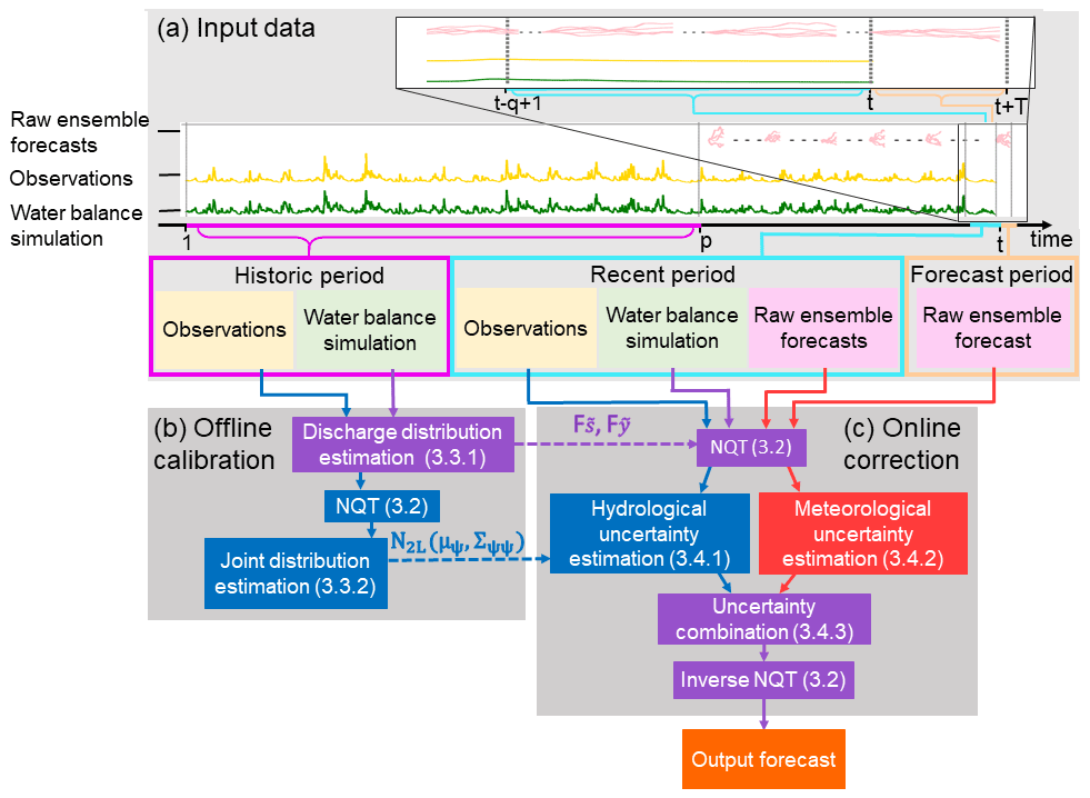
Figure 1 Flow chart describing the post-processing method at a station. (a) Input data are separated by time period (historic period: fuchsia, recent period: cyan, forecast period: peach) and by data type (observations: yellow, water balance simulations: green, raw ensemble forecasts: pink). The top time series is a magnification of the bottom time series for the period $t-q+\mathrm{1}$ to t+T. The historic period has length p. For a forecast produced at time t, the recent period starts at time $t-q+\mathrm{1}$ and the forecast period ends at time t+T. (b) Offline calibration steps. (c) Online correction steps. NQT is the normal quantile transform. Blue and red arrows and boxes show the data and methods used to account for the hydrological uncertainty and the meteorological uncertainty, respectively. Data and methods used to account for both the hydrological and meteorological uncertainties are shown in purple. Dashed arrows show data stored in the station model such as the cumulative distribution functions of the water balance simulation and observations, denoted $F_{\stackrel{\mathrm{̃}}{s}}$ and $F_{\stackrel{\mathrm{̃}}{y}}$, respectively, and the joint distribution between the water balance simulation and observations, denoted N_2L(µ_ψ,Σ_ψψ). Section numbers given in parentheses contain more details.

3.1 Notation

In this section notation and definitions used throughout the paper are introduced. The aim of post-processing is to correct the errors and account for the uncertainty that may be present in a forecast. As described in Sect. 2, the EFAS produces ensemble streamflow forecasts for the whole of Europe on a 5 km grid with 6-hourly timesteps. However, post-processing is performed at daily timesteps and only at stations for which near-real-time and historic river discharge observations are available. Therefore, the discharge values corresponding to the grid boxes representing the locations of the stations are extracted and temporally aggregated to daily timesteps. This creates a separate streamflow forecast for each station, and it is these single station forecasts that are henceforth referred to as the raw forecasts. The post-processing method evaluated in this paper is applied separately at each station, creating a corresponding post-processed forecast for each raw forecast.

The input data shown in Fig. 1a are the input data required for the post-processing of a single raw forecast (i.e. for one station). As shown, the input data can be separated into three time periods. These time periods are henceforth referred to (from left to right in Fig. 1a) as the historic period, the recent period, and the forecast period. The length of the historic period, denoted p, varies between stations depending on the length of the historic observational record available. However, a minimum of 2 years of observations since 1991 is required for the offline calibration. For a forecast produced at time t, the recent period has q timesteps and extends from time $t-q+\mathrm{1}$ to time t. The forecast period extends from time t+1 to time t+T for a forecast with a maximum lead time of T timesteps. The length of the recent period and the forecast period combined is $L=q+T$. For convenience, we introduce a timestep notation of the form t_i:t_j to represent all timesteps between time t_i and time t_j, i.e. t_i : t_j means $t_i,t_i+\mathrm{1},t_i+\mathrm{2},\mathrm{\dots }{t}_j-\mathrm{1},t_j$.

The raw ensemble forecast that is post-processed is the only data available in the forecast period. This forecast is produced at time t and has M ensemble members and a maximum lead time of T timesteps. The full ensemble forecast is represented by a matrix, denoted ${\stackrel{\mathrm{̃}}{\mathbf{x}}}_t(t+\mathrm{1}:t+T)\in {\mathbb{R}}^{T\times M}$, where each column corresponds to an ensemble member and contains a vector of discharge values for each timestep in the forecast period. Throughout the paper, the tilde notation indicates that the discharge values are in physical space, whereas discharge values without the tilde are in the standard Normal space (see Sect. 3.2). The subscript t indicates the forecast production time, and the range of timesteps for which discharge values are available is shown using the timestep notation. The raw ensemble forecasts from the recent period are denoted using similar notation such that, for example, the forecast produced at $t-q+\mathrm{1}$ is denoted ${\stackrel{\mathrm{̃}}{\mathbf{x}}}_{t-q+\mathrm{1}}(t-q+\mathrm{2}:t-q+\mathrm{1}+T)\in {\mathbb{R}}^{T\times M}$. All forecasts are from the same forecasting system, and so all have M ensemble members and maximum lead times of T timesteps.

The time series of observations for a single station is denoted by the vector $\stackrel{\mathrm{̃}}{\mathit{y}}$, where each element represents a daily discharge observation. The observations in the historic period are used in the offline calibration (see Fig. 1b and Sect. 3.3) and are denoted $\stackrel{\mathrm{̃}}{\mathit{y}}(\mathrm{1}:p)\in {\mathbb{R}}^p$, where the timestep notation is used to show the range of timesteps for which observations are available. This vector is the same for all forecasts for this station as the station model is not updated between forecasts. The observations in the recent period (the q timesteps up to the production time of the forecast) are used in the online correction (see Fig. 1c and Sect. 3.4) and are denoted $\stackrel{\mathrm{̃}}{\mathit{y}}(t-q+\mathrm{1}:t)\in {\mathbb{R}}^q$. Since $\stackrel{\mathrm{̃}}{\mathit{y}}(t-q+\mathrm{1}:t)$ is a function of t, the observations in this vector are different for each forecast production time.

Similarly, the time series of the water balance simulation, denoted by the vector $\stackrel{\mathrm{̃}}{\mathit{s}}$, is used in both the offline calibration and the online correction. Each element of the vector represents a daily water balance simulation value calculated by forcing LISFLOOD with meteorological observations (see Sect. 2). The water balance simulation values from the historic period, $\stackrel{\mathrm{̃}}{\mathit{s}}(\mathrm{1}:p)$, are selected to correspond to the timesteps of the p observations from the same period. The water balance simulation values from the recent period are denoted $\stackrel{\mathrm{̃}}{\mathit{s}}(t-q+\mathrm{1}:t)$ and are dependent on the forecast production time, t.

3.2 NQT

The methods used in this post-processing method utilise the properties of the Gaussian distribution, but discharge values usually have highly skewed non-Gaussian distributions (Hemri, 2018). Therefore, the NQT is used to transform the discharge data to the standard Normal distribution, which has a mean of 0 and a variance of 1, denoted N(0,1). The NQT is applied separately to all input data (observed, simulated, and forecast) for a given station; therefore, it is defined here for any scalar discharge value $\stackrel{\mathrm{̃}}{\mathit{\eta }}$.

The NQT defines a one-to-one map between the quantiles of the cumulative distribution function (CDF) of the discharge distribution in physical space, $F_{\stackrel{\mathrm{̃}}{\mathit{\eta }}}\left(\stackrel{\mathrm{̃}}{\mathit{\eta }}\right)$, and the CDF of the standard Normal distribution, Q(η). The scalar function $F_{\stackrel{\mathrm{̃}}{\mathit{\eta }}}$ is dependent on whether $\stackrel{\mathrm{̃}}{\mathit{\eta }}$ represents a modelled discharge value (simulated or forecast) or an observed discharge value. The calculation of the discharge distributions and their subsequent CDFs are described in Sect. 3.3.1. The NQT transforms each scalar discharge value such that

$$\begin{array}{}\text{(1)}& \mathit{\eta }=Q^{-\mathrm{1}}\left(F_{\stackrel{\mathrm{̃}}{\mathit{\eta }}}\left(\stackrel{\mathrm{̃}}{\mathit{\eta }}\right)\right).\end{array}$$

After the forecast values have been adjusted by the post-processing method, the inverse NQT,

$$\begin{array}{}\text{(2)}& \stackrel{\mathrm{̃}}{\mathit{\eta }}=F_{\stackrel{\mathrm{̃}}{\mathit{\eta }}}^{-\mathrm{1}}\left(Q\left(\mathit{\eta }\right)\right),\end{array}$$

is applied to transform the discharge values from the standard Normal space back to the physical space (see Fig. 1c).

3.3 Offline calibration

The offline calibration (see Fig. 1b) has two main aims: to determine the distributions of the observed, $\stackrel{\mathrm{̃}}{\mathit{y}}$, and simulated, $\stackrel{\mathrm{̃}}{\mathit{s}}$, discharge values at a station and to define the joint distribution between the transformed observations, y, and the transformed water balance simulation, s. These distributions are then stored in the station model for use in the online post-processing step (shown by dashed lines in Fig. 1). The input data required for the offline calibration are a historic record of observations for the station, denoted by the vector $\stackrel{\mathrm{̃}}{\mathit{y}}(\mathrm{1}:p)\in {\mathbb{R}}^p$, and, for the same period, a historic time series of the water balance simulation for the grid box representing the location of the station, denoted by the vector $\stackrel{\mathrm{̃}}{\mathit{s}}(\mathrm{1}:p)\in {\mathbb{R}}^p$. The length of these vectors, p, is equal to the number of data points in the historic records and varies between stations. A minimum of 2 years of historical data is required to guarantee that p>>L (see Sect. 3.1).

3.3.1 Discharge distribution approximation

The NQT requires the CDF of the observed and simulated discharge values in physical space, denoted $F_{\stackrel{\mathrm{̃}}{y}}$ and $F_{\stackrel{\mathrm{̃}}{s}}$, respectively, to be defined. This section describes the approach used to estimate these functions. First, the discharge density distributions are estimated using the observations, $\stackrel{\mathrm{̃}}{\mathit{y}}(\mathrm{1}:p)\in {\mathbb{R}}^p$, and the water balance simulation values, $\stackrel{\mathrm{̃}}{\mathit{s}}(\mathrm{1}:p)\in {\mathbb{R}}^p$, from the historic period. These historic time series are often only a few years long and therefore may not represent the full discharge distribution due to the relative rarity of larger discharge values. To avoid the issues that short time series commonly cause in the inverse NQT (discussed in Bogner et al., 2012) rather than using the empirical distribution as was done in the original MCP method (Todini, 2008), an approximation of the discharge distribution is determined using a method similar to that presented in MacDonald et al. (2011). The approximation method applies kernel density estimation (KDE) to the bulk of the distribution (Węglarczyk, 2018) and fits a generalised type-II Pareto distribution (GPD) to the upper tail (Kleiber and Kotz, 2003) to create a composite distribution (see Fig. 2). The GPD is an extreme value distribution that is fully defined by three parameters: the location parameter a, the scale parameter b, and the shape parameter c. Within this composite distribution the location parameter also serves as the breakpoint which separates the kernel density and the GPD and is shown in Fig. 2. The parameters of the GPD are determined using the concentrated likelihood method (see steps 4–6 below). The concentrated likelihood method allows the maximum likelihood estimates of multiple parameters to be determined by first expressing one parameter in terms of the others (Takeshi, 1985). The time series of discharge values, $\stackrel{\mathrm{̃}}{\mathit{\eta }}(\mathrm{1}:p)\in {\mathbb{R}}^p$, is used here to describe the distribution approximation which is implemented as follows.

1. All values in the time series, $\stackrel{\mathrm{̃}}{\mathit{\eta }}$, are sorted into descending order, with ${\stackrel{\mathrm{̃}}{\mathit{\eta }}}_{\mathrm{1}}$ denoting the largest value in the time series, ${\stackrel{\mathrm{̃}}{\mathit{\eta }}}_{\mathrm{2}}$ denoting the second-largest value, and so on.

2. A Gaussian kernel is centred at each data point such that

   $$\begin{array}{}\text{(3)}& K_i\left(x\right)={\displaystyle \frac{\mathrm{1}}{{\mathit{\sigma }}_{\stackrel{\mathrm{̃}}{\mathit{\eta }}}\sqrt{\mathrm{2}\mathit{\pi }}}}{e}^{-(x-{\stackrel{\mathrm{̃}}{\mathit{\eta }}}_i{)}^{\mathrm{2}}/\mathrm{2}{\mathit{\sigma }}_{\stackrel{\mathrm{̃}}{\mathit{\eta }}}^{\mathrm{2}}},\end{array}$$

   where K_i is the kernel centred at ${\stackrel{\mathrm{̃}}{\mathit{\eta }}}_i$, and ${\mathit{\sigma }}_{\stackrel{\mathrm{̃}}{\mathit{\eta }}}$ is Silverman's “rule of thumb” bandwidth (Silverman, 1984). The bandwidth is calculated using the built-in R function bw.nrd0 (R Core Team, 2019; Venables and Ripley, 2002) and all values in the time series, $\stackrel{\mathrm{̃}}{\mathit{\eta }}$.

3. The kernel density is estimated using a leave-one-out approach such that the density at ${\stackrel{\mathrm{̃}}{\mathit{\eta }}}_j$ is

   $$\begin{array}{}\text{(4)}& P\left({\stackrel{\mathrm{̃}}{\mathit{\eta }}}_j\right)={\displaystyle \frac{\mathrm{1}}{p-\mathrm{1}}}\sum _{i\ne j}{K}_i\left({\stackrel{\mathrm{̃}}{\mathit{\eta }}}_j\right).\end{array}$$

   This makes sure that the density is not over-fitted to any individual data point.

4. To guarantee data points in the tail, the largest 10 values are always assumed to be in the upper tail of the distribution (within the GPD), and the next 990 values (i.e. ${\stackrel{\mathrm{̃}}{\mathit{\eta }}}_{\mathrm{11}}$ to ${\stackrel{\mathrm{̃}}{\mathit{\eta }}}_{\mathrm{1000}}$) are each tried as the location parameter, a, of the GPD. If there are fewer than 1000 data points (i.e. p<1000), then all data points are tried as the location parameter.

5. For each test value of a:

   • i.

     The scale parameter, b, is determined analytically by the constraints that the density distribution must be equal at the breakpoint for both the GPD and the KDE distribution, and the integral of the full density distribution function with respect to discharge must be equal to 1.

   • ii.

     The shape parameter, c, is determined numerically by finding the maximum likelihood estimate, given the values of a and b, within the limits of $-\mathrm{1}\le c\ge \frac{b}{{\stackrel{\mathrm{̃}}{\mathit{\eta }}}_{\mathrm{1}}}$ (de Zea Bermudez and Kotz, 2010). The upper limit guarantees the upper bound of the distribution is greater than the maximum value in the time series, ${\stackrel{\mathrm{̃}}{\mathit{\eta }}}_{\mathrm{1}}$, and the lower limit constrains the number of values considered to reduce the computational time required.

   For stations with p>1000, this produces 990 sets of parameters.

6. The full distribution is the combination of the KDE and GPD weighted by their contribution to the total density, $F_{\stackrel{\mathrm{̃}}{\mathit{\eta }}}\left(a\right)$ and $\mathrm{1}-F_{\stackrel{\mathrm{̃}}{\mathit{\eta }}}\left(a\right)$, respectively (MacDonald et al., 2011). The likelihood function for the full distribution is used to determine the maximum likelihood estimate of the location parameter, a, given the values of b and c that were calculated in step 5 for each possible value of a. This results in the most likely set of parameters (a_ML, b_ML, c_ML) to define the GPD fitted to the upper tail of the distribution.

The six steps outlined above are applied separately to both the simulated time series, $\stackrel{\mathrm{̃}}{\mathit{s}}(\mathrm{1}:p)$, and the observed time series, $\stackrel{\mathrm{̃}}{\mathit{y}}(\mathrm{1}:p)$. Figure 2 illustrates the approximation method for the simulated discharge distribution for a single station.

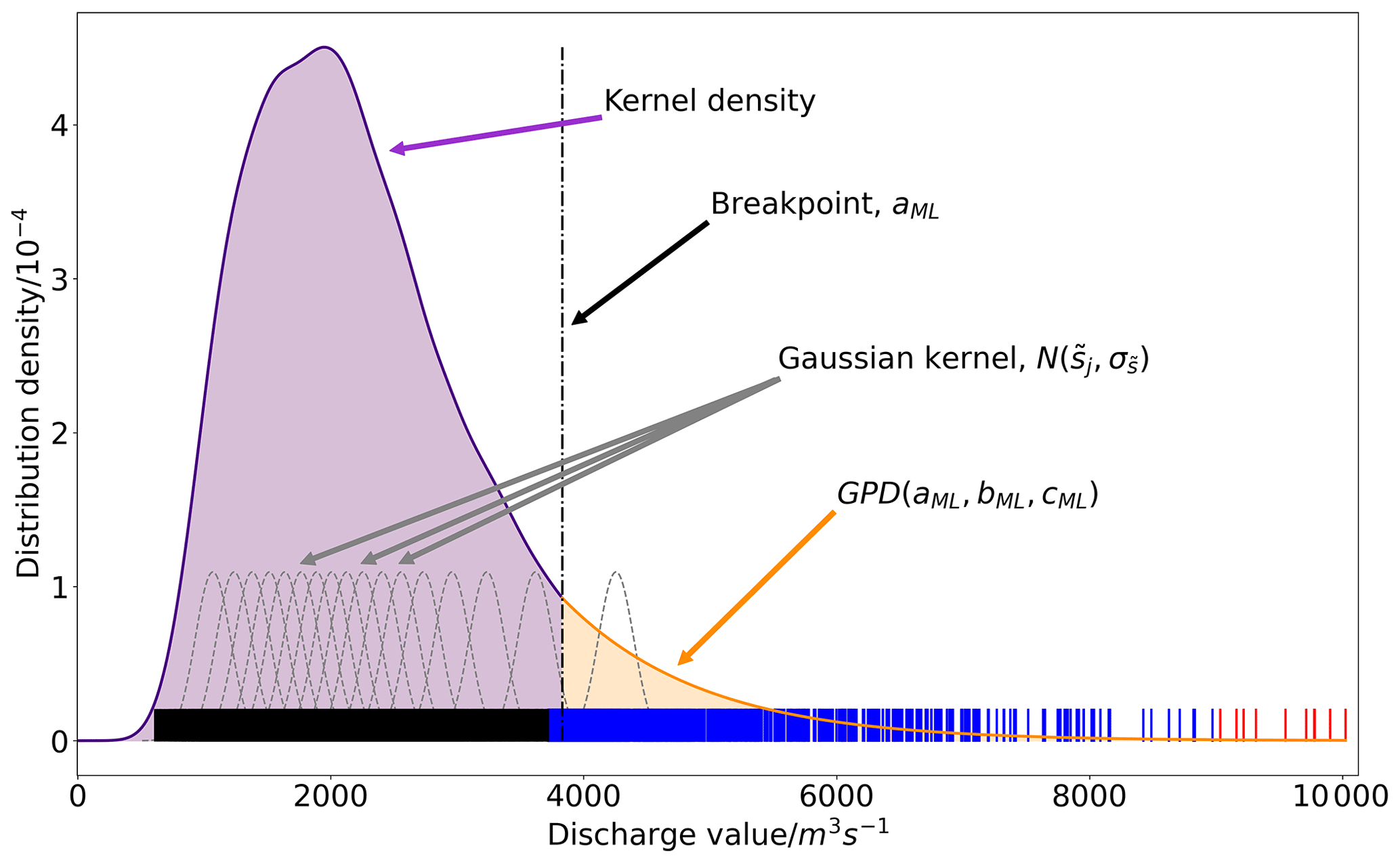
Figure 2 Schematic of the distribution approximation method. All data points are shown by the short solid lines. The largest 10 data points are red (always in the upper tail), the next 990 largest data points are blue (tried as the location parameter), and the remaining data points are black. Gaussian kernels (grey dashed lines) are used to calculate the kernel density (purple line). For clarity, only the kernels centred at every 500th data point are plotted. The upper tail is fitted with a generalised type-II Pareto distribution (orange line). The breakpoint (dot-dashed black line) defines the separation between the two distributions. The integral of the density distribution function with respect to discharge (the sum of the purple- and orange-shaded areas) equals 1.

Once the variables that define the discharge density distribution, namely ${\mathit{\sigma }}_{\stackrel{\mathrm{̃}}{\mathit{\eta }}}$, a_ML, b_ML, and c_ML, have been determined, the CDF can be calculated analytically for both the observed and simulated discharge distributions. All input data (for both the online and offline parts of the method) must be transformed to the standard Normal space using the NQT. However, it is too computationally expensive to calculate the analytical CDF for each data point. To increase the computational efficiency of the NQT, the KDE parts of the CDFs are approximated as piecewise linear functions. Each data point in the historic time series is considered a knot (a boundary point between pieces of the piecewise function). The CDF values at the mid-points between knots are approximated using linear interpolation. If the approximated and analytical CDFs differ by more than $\mathrm{1}\times {\mathrm{10}}^{-\mathrm{5}}$, then the mid-points are added as additional knots. The process is repeated until the approximated CDF is accurate to within $\mathrm{1}\times {\mathrm{10}}^{-\mathrm{5}}$. Ensuring that the CDF for any discharge value can be determined using linear interpolation makes the application of the NQT more efficient.

3.3.2 Joint distribution estimation

This section describes the calculation of the joint distribution used in the online hydrological uncertainty estimation (see Sect. 3.4.1). First, the discharge distributions defined in Sect. 3.3.1 are used within the NQT to transform the historic observations and water balance simulation to the standard Normal space (see Fig. 1b). This allows the joint distribution to be calculated as a multi-variate Gaussian distribution. The joint distribution is defined between the observations and water balance simulation values at L timesteps, which, as noted in Sect. 3.1, is equal to the length of the recent period (q timesteps) and forecast period (T timesteps) combined. The L timesteps are defined relative to a timestep k such that the joint distribution is a 2L-dimensional distribution that describes the relationship between the observations, $\mathit{y}(k-q+\mathrm{1}:k+T)$, and the water balance simulation values, $\mathit{s}(k-q+\mathrm{1}:k+T)$. To ease notation, we introduce the vector ϕ(t_i:t_j), here defined generally for arbitrary timesteps, which includes the observed and simulated discharge values for all timesteps between timestep t_i and timestep t_j, such that

$$\begin{array}{}\text{(5)}& \mathit{\varphi }(t_i:t_j)=\left(\begin{array}{c}\mathit{y}(t_i:t_j)\\ \mathit{s}(t_i:t_j)\end{array}\right).\end{array}$$

Following on from Eq. 5, we define the vector ψ∈ℝ^2L:

$$\begin{array}{}\text{(6)}& \begin{array}{rl}\mathit{\psi }(k-q+\mathrm{1}:k+T)& =\left(\begin{array}{c}\mathit{\varphi }(k-q+\mathrm{1}:k)\\ \mathit{\varphi }(k+\mathrm{1}:k+T)\end{array}\right)\\ & =\left(\begin{array}{c}\mathit{y}(k-q+\mathrm{1}:k)\\ \mathit{s}(k-q+\mathrm{1}:k)\\ \mathit{y}(k+\mathrm{1}:k+T)\\ \mathit{s}(k+\mathrm{1}:k+T)\end{array}\right)\in {\mathbb{R}}^{\mathrm{2}L}.\end{array}\end{array}$$

The splitting of the observed and simulated variables into two distinct time periods is discussed below. The joint distribution can now be defined in terms of $\mathit{\psi }(k-q+\mathrm{1}:k+T)$.

The joint distribution is denoted $N_{\mathrm{2}L}\left({\mathit{\mu }}_{\mathit{\psi }}\right(k-q+\mathrm{1}:k+T),{\mathbf{\Sigma }}_{\mathit{\psi }\mathit{\psi }}(k-q+\mathrm{1}:k+T,k-q+\mathrm{1}:k+T\left)\right)$, where the subscript 2L indicates its dimensions and the subscript ψ indicates that the distribution is for both the observed and simulated variables. The distribution is fully defined by its mean, ${\mathit{\mu }}_{\mathit{\psi }}(k-q+\mathrm{1}:k+T)\in {\mathbb{R}}^{\mathrm{2}L}$, and covariance matrix, ${\mathbf{\Sigma }}_{\mathit{\psi }\mathit{\psi }}(k-q+\mathrm{1}:k+T,k-q+\mathrm{1}:k+T)\in {\mathbb{R}}^{\mathrm{2}L\times \mathrm{2}L}$. Since both the observed and simulated historic time series have been transformed into the standard Normal space, the mean discharge value is 0 for both distributions, and therefore the mean vector is defined as ${\mathit{\mu }}_{\mathit{\psi }}(k-q+\mathrm{1}:k+T)=\mathbf{0}$. The covariance matrix of the joint distribution is calculated as

$$\begin{array}{}\text{(7)}& \begin{array}{rl}{\mathbf{\Sigma }}_{\mathit{\psi }\mathit{\psi }}& (k-q+\mathrm{1}:k+T,k-q+\mathrm{1}:k+T)\\ & ={\displaystyle \frac{\mathrm{1}}{p-L}}\sum _{k=q}^{p-T}\mathit{\psi }(k-q+\mathrm{1}:k+T)\\ & \times \mathit{\psi }(k-q+\mathrm{1}:k+T{)}^{\mathrm{T}}\in {\mathbb{R}}^{\mathrm{2}L\times \mathrm{2}L},\end{array}\end{array}$$

where $\mathit{\psi }(k-q+\mathrm{1}:k+T)$ is defined as in Eq. 6 for each timestep, k, in the historic period. Since many stations have short time series, the impact of the seasonal cycle on the joint distribution is not considered. Additionally, any spurious correlations resulting from these short time series are not currently treated.

To ensure that the covariance matrix, ${\mathbf{\Sigma }}_{\mathit{\psi }\mathit{\psi }}(k-q+\mathrm{1}:k+T,k-q+\mathrm{1}:k+T)$, is positive definite, the minimum eigenvalue method is used (Tabeart et al., 2020). The covariance matrix is decomposed into the eigenvalues and eigenvectors. A minimum eigenvalue threshold is set to $\mathrm{1}\times {\mathrm{10}}^{-\mathrm{7}}{\mathit{\lambda }}_{\mathrm{1}}$, where λ₁ is the largest eigenvalue. All eigenvalues below this threshold are set to the threshold. The matrix is then reconstructed and scaled to match the variance of the original covariance matrix.

As mentioned, the joint distribution is used in the estimation of the hydrological uncertainty in the online part of the post-processing method (see Sect. 3.4.1). If the joint distribution is defined such that k is equal to the production time of a forecast, then timesteps $k-q+\mathrm{1}$ to k correspond to the recent period and timesteps k+1 to k+T correspond to the forecast period. Therefore, the joint distribution can be used to condition the unknown observations and water balance simulation values in the forecast period on the known observations and water balance simulation values from the recent period. Here, we introduce notation that is used to split the joint distribution into the variables corresponding to each of these two periods. First, the mean vector is split by timestep (as in Eq. 6) such that

$$\begin{array}{}\text{(8)}& {\mathit{\mu }}_{\mathit{\psi }}(k-q+\mathrm{1}:k+T)=\left(\begin{array}{c}{\mathit{\mu }}_{\mathit{\varphi }}(k-q+\mathrm{1}:k)\\ {\mathit{\mu }}_{\mathit{\varphi }}(k+\mathrm{1}:k+T)\end{array}\right),\end{array}$$

where ${\mathit{\mu }}_{\mathit{\varphi }}(k-q+\mathrm{1}:k)$ represents the mean of the variables in the recent period for a forecast produced at time k and ${\mathit{\mu }}_{\mathit{\varphi }}(k+\mathrm{1}:k+T)$ represents the mean of the variables in the forecast period. The subscript ϕ indicates that the distribution is for the observed and simulated variables for a single time period, following the structure shown in Eq. 5, rather than for both time periods as indicated by the subscript ψ. The covariance matrix can be expressed as

$$\begin{array}{}\text{(9)}& \begin{array}{rl}& {\mathbf{\Sigma }}_{\mathit{\psi }\mathit{\psi }}(k-q+\mathrm{1}:k+T,k-q+\mathrm{1}:k+T)=\\ & \left(\begin{array}{ll}{\mathbf{\Sigma }}_{\mathit{\varphi }\mathit{\varphi }}(k-q+\mathrm{1}:k,k-q+\mathrm{1}:k)& {\mathbf{\Sigma }}_{\mathit{\varphi }\mathit{\varphi }}(k-q+\mathrm{1}:k,k+\mathrm{1}:k+T)\\ {\mathbf{\Sigma }}_{\mathit{\varphi }\mathit{\varphi }}(k+\mathrm{1}:k+T,k-q+\mathrm{1}:k)& {\mathbf{\Sigma }}_{\mathit{\varphi }\mathit{\varphi }}(k+\mathrm{1}:k+T,k+\mathrm{1}:k+T)\end{array}\right),\end{array}\end{array}$$

where ${\mathbf{\Sigma }}_{\mathit{\varphi }\mathit{\varphi }}(k-q+\mathrm{1}:k,k-q+\mathrm{1}:k)$ and ${\mathbf{\Sigma }}_{\mathit{\varphi }\mathit{\varphi }}(k+\mathrm{1}:k+T,k+\mathrm{1}:k+T)$ are the covariance matrices for variables in the recent and forecast periods, respectively, and ${\mathbf{\Sigma }}_{\mathit{\varphi }\mathit{\varphi }}(k-q+\mathrm{1}:k,k+\mathrm{1}:k+T)$ and ${\mathbf{\Sigma }}_{\mathit{\varphi }\mathit{\varphi }}(k+\mathrm{1}:k+T,k-q+\mathrm{1}:k)$ represent the cross-covariance matrices of variables in both time periods.

These sub-matrices can be further decomposed into the components referring to the observed and simulated variables such that, for example,

$$\begin{array}{}\text{(10)}& \begin{array}{rl}& {\mathbf{\Sigma }}_{\mathit{\varphi }\mathit{\varphi }}(k+\mathrm{1}:k+T,k+\mathrm{1}:k+T)=\\ & \left(\begin{array}{ll}{\mathbf{\Sigma }}_{\mathit{y}\mathit{y}}(k+\mathrm{1}:k+T,k+\mathrm{1}:k+T)& {\mathbf{\Sigma }}_{\mathit{y}\mathit{s}}(k+\mathrm{1}:k+T,k+\mathrm{1}:k+T)\\ {\mathbf{\Sigma }}_{\mathit{s}\mathit{y}}(k+\mathrm{1}:k+T,k+\mathrm{1}:k+T)& {\mathbf{\Sigma }}_{\mathit{s}\mathit{s}}(k+\mathrm{1}:k+T,k+\mathrm{1}:k+T)\end{array}\right),\end{array}\end{array}$$

where the subscripts y and s indicate that the distribution refers to the observed and simulated variables, respectively (in contrast to the subscript ϕ, which indicates that both observed and simulated variables are included). The mean vector can also be split in this way such that

$$\begin{array}{}\text{(11)}& {\mathit{\mu }}_{\mathit{\varphi }}(k+\mathrm{1}:k+T)=\left(\begin{array}{l}{\mathit{\mu }}_{\mathit{y}}(k+\mathrm{1}:k+T)\\ {\mathit{\mu }}_{\mathit{s}}(k+\mathrm{1}:k+T)\end{array}\right).\end{array}$$

3.4 Online correction

This section describes the online correction part of the post-processing method (see Fig. 1c). The online correction quantifies and combines the hydrological and meteorological uncertainties for a specific forecast to produce the final probabilistic forecast. This forecast is produced at time t and has a maximum lead time of T days, ${\stackrel{\mathrm{̃}}{\mathbf{x}}}_{\mathbf{t}}(t+\mathrm{1}:t+T)\in {\mathbb{R}}^{M\times T}$ (see Sect. 3.1 for a description of the notation). As shown in Fig. 1, as well as the current forecast produced at time t, the online correction requires the following input data from the recent period:

• observations for the station, $\stackrel{\mathrm{̃}}{\mathit{y}}(t-q+\mathrm{1}:t)\in {\mathbb{R}}^q$,

• the water balance simulation for the grid box containing the station's location, $\stackrel{\mathrm{̃}}{\mathit{s}}(t-q+\mathrm{1}:t)\in {\mathbb{R}}^q$, and

• a set of ensemble streamflow forecasts (from the same system as the forecast ${\stackrel{\mathrm{̃}}{\mathbf{x}}}_{\mathbf{t}}$) for the grid box containing the station's location, $\mathit{\{}{\stackrel{\mathrm{̃}}{\mathbf{x}}}_{\mathbf{t}-\mathbf{q}+\mathbf{1}},{\stackrel{\mathrm{̃}}{\mathbf{x}}}_{\mathbf{t}-\mathbf{q}+\mathbf{2}},\mathrm{\dots },{\stackrel{\mathrm{̃}}{\mathbf{x}}}_{\mathbf{t}-\mathbf{1}}\mathit{\}}$.

Previous work used tuning experiments to determine that a recent period of length 40 d (i.e. q=40) was most appropriate (Paul Smith, personal communication, 2020). All the input data are transformed to the standard Normal space using the NQT (see Eq. 1) and the CDFs determined in the offline calibration (see Sect. 3.3) and stored in the station model, $F_{\stackrel{\mathrm{̃}}{y}}$ and $F_{\stackrel{\mathrm{̃}}{s}}$. The observations are transformed using $F_{\stackrel{\mathrm{̃}}{y}}$, and the water balance simulation and forecasts are transformed using $F_{\stackrel{\mathrm{̃}}{s}}$. The following sections provide more detail on the methods used to account for the uncertainties and are performed within the standard Normal space. For simplicity, it is assumed that all data are available and that there are no data latency issues such that the most recent observation available is $\stackrel{\mathrm{̃}}{y}\left(t\right)$ for the timestep when the forecast is produced. In practice, some observations from the recent period may not be available, and additionally the operational system does have a data latency of approximately 1 d.

3.4.1 Hydrological uncertainties

The hydrological uncertainty is quantified using a MCP method which uses the discharge values from the recent period and the joint distribution, N_2L(μ_ψ,Σ_ψψ), defined in the offline calibration (see Sect. 3.3.2). The joint distribution defines the relationship between the observations and water balance simulation across $L=q+T$ timesteps. The hydrological uncertainty is estimated by conditioning the unknown observations and water balance simulation values in the forecast period on the known observed and simulated discharge values from the recent period using the joint distribution. First, the station observations and water balance simulations from the recent period are combined into a single vector, $\left(\mathit{\varphi }\right(t-q+\mathrm{1}:t)$, as defined in Eq. 5.

In Sect. 3.3.2, the L timesteps of the joint distribution were defined relative to a timestep k. Here, k is set equal to the production time of the forecast, t, such that the timesteps from $t-q+\mathrm{1}$ to t correspond to the recent period and the timesteps from t+1 to t+T correspond to the forecast period. Thus, the mean vector of the joint distribution can be expressed, as discussed in Sect. 3.3.2, as

$$\begin{array}{}\text{(12)}& {\mathit{\mu }}_{\mathit{\psi }}(t-q+\mathrm{1}:t+T)=\left(\begin{array}{c}{\mathit{\mu }}_{\mathit{\varphi }}(t-q+\mathrm{1}:t)\\ {\mathit{\mu }}_{\mathit{\varphi }}(t+\mathrm{1}:t+T)\end{array}\right),\end{array}$$

where ${\mathit{\mu }}_{\mathit{\varphi }}(t-q+\mathrm{1}:t)$ represents the mean of the variables (both observations and water balance simulation) in the recent period, for which we have known values, $\mathit{\varphi }(t-q+\mathrm{1}:t)$, and ${\mathit{\mu }}_{\mathit{\varphi }}(t+\mathrm{1}:t+T)$ represents the mean of the variables in the forecast period, which we are required to predict.

The sub-matrices of the covariance matrix of the joint distribution that were defined in Eq. 10 are also positioned relative to timestep t, such that

$$\begin{array}{}\text{(13)}& \begin{array}{rl}& {\mathbf{\Sigma }}_{\mathit{\psi }\mathit{\psi }}(t-q+\mathrm{1}:t+T,t-q+\mathrm{1}:t+T)=\\ & \left(\begin{array}{ll}{\mathbf{\Sigma }}_{\mathit{\varphi }\mathit{\varphi }}(t-q+\mathrm{1}:t,t-q+\mathrm{1}:t)& {\mathbf{\Sigma }}_{\mathit{\varphi }\mathit{\varphi }}(t-q+\mathrm{1}:t,t+\mathrm{1}:t+T)\\ {\mathbf{\Sigma }}_{\mathit{\varphi }\mathit{\varphi }}(t+\mathrm{1}:t+T,t-q+\mathrm{1}:t)& {\mathbf{\Sigma }}_{\mathit{\varphi }\mathit{\varphi }}(t+\mathrm{1}:t+T,t+\mathrm{1}:t+T)\end{array}\right).\end{array}\end{array}$$

By positioning the joint distribution in this way, ${\mathit{\mu }}_{\mathit{\varphi }}(t+\mathrm{1}:t+T)\in {\mathbb{R}}^{\mathrm{2}T}$ and the sub-matrix ${\mathbf{\Sigma }}_{\mathit{\varphi }\mathit{\varphi }}(t+\mathrm{1}:t+T,t+\mathrm{1}:t+T)\in {\mathbb{R}}^{\mathrm{2}T\times \mathrm{2}T}$ create a climatological forecast for the observations and water balance simulation in the standard Normal space. It is this climatological forecast that is conditioned on the discharge values from the recent period.

The conditional distribution of the unknown discharge values in the forecast period conditioned on the known discharge values in the recent period, denoted $N_{\mathrm{2}T}\left({\widehat{\mathit{\mu }}}_{\mathit{\varphi }}\right(t+\mathrm{1}:t+T),{\widehat{\mathbf{\Sigma }}}_{\mathit{\varphi }\mathit{\varphi }}(t+\mathrm{1}:t+T,t+\mathrm{1}:t+T\left)\right)$, is calculated using the properties of a multi-variate Gaussian joint distribution (Dey and Rao, 2006) such that

$$\begin{array}{}\text{(14)}& \begin{array}{rl}{\widehat{\mathit{\mu }}}_{\mathit{\varphi }}& (t+\mathrm{1}:t+T)={\mathit{\mu }}_{\mathit{\varphi }}(t+\mathrm{1}:t+T)\\ & +{\mathbf{\Sigma }}_{\mathit{\varphi }\mathit{\varphi }}(t+\mathrm{1}:t+T,t-q+\mathrm{1}:t)\\ & \times {\mathbf{\Sigma }}_{\mathit{\varphi }\mathit{\varphi }}(t-q+\mathrm{1}:t,t-q+\mathrm{1}:t{)}^{-\mathrm{1}}\\ & \times \left(\mathit{\varphi }(t-q+\mathrm{1}:t)-{\mathit{\mu }}_{\mathit{\varphi }}(t-q+\mathrm{1}:t)\right)\end{array}\end{array}$$

and

$$\begin{array}{}\text{(15)}& \begin{array}{rl}{\widehat{\mathbf{\Sigma }}}_{\mathit{\varphi }\mathit{\varphi }}& (t+\mathrm{1}:t+T,t+\mathrm{1}:t+T)\\ & ={\mathbf{\Sigma }}_{\mathit{\varphi }\mathit{\varphi }}(t+\mathrm{1}:t+T,t+\mathrm{1}:t+T)\\ & -{\mathbf{\Sigma }}_{\mathit{\varphi }\mathit{\varphi }}(t+\mathrm{1}:t+T,t-q+\mathrm{1}:t)\\ & \times {\mathbf{\Sigma }}_{\mathit{\varphi }\mathit{\varphi }}^{-\mathbf{1}}(t-q+\mathrm{1}:t,t-q+\mathrm{1}:t)\\ & \times {\mathbf{\Sigma }}_{\mathit{\varphi }\mathit{\varphi }}(t-q+\mathrm{1}:t,t+\mathrm{1}:t+T),\end{array}\end{array}$$

where the hat notation indicates that it is conditioned on the discharge values from the recent period.

The resulting predicted distribution, $N_{\mathrm{2}T}\left({\widehat{\mathit{\mu }}}_{\mathit{\varphi }}\right(t+\mathrm{1}:t+T),{\widehat{\mathbf{\Sigma }}}_{\mathit{\varphi }\mathit{\varphi }}(t+\mathrm{1}:t+T,t+\mathrm{1}:t+T\left)\right)$, is referred to as the hydrological uncertainty distribution and can be partitioned into two T-dimensional forecasts, one for the water balance simulation and one for the unknown observations in the forecast period, such that

$$\begin{array}{}\text{(16)}& \begin{array}{rl}& \left[\begin{array}{l}\mathit{y}(t+\mathrm{1}:t+T)\\ \mathit{s}(t+\mathrm{1}:t+T)\end{array}\right]\sim N_{\mathrm{2}T}\left(\left[\begin{array}{l}{\widehat{\mathit{\mu }}}_{\mathit{y}}(t+\mathrm{1}:t+T)\\ {\widehat{\mathit{\mu }}}_{\mathit{s}}(t+\mathrm{1}:t+T)\end{array}\right],\right.\\ & \left.\left[\begin{array}{ll}{\widehat{\mathbf{\Sigma }}}_{\mathit{y}\mathit{y}}(t+\mathrm{1}:t+T,t+\mathrm{1}:t+T)& {\widehat{\mathbf{\Sigma }}}_{\mathit{y}\mathit{s}}(t+\mathrm{1}:t+T,t+\mathrm{1}:t+T)\\ {\widehat{\mathbf{\Sigma }}}_{\mathit{s}\mathit{y}}(t+\mathrm{1}:t+T,t+\mathrm{1}:t+T)& {\widehat{\mathbf{\Sigma }}}_{\mathit{s}\mathit{s}}(t+\mathrm{1}:t+T,t+\mathrm{1}:t+T)\end{array}\right]\right).\end{array}\end{array}$$

The subscripts y and s indicate that the distribution refers to the observed and simulated variables, respectively.

3.4.2 Meteorological uncertainty

This section describes the part of the online correction that estimates the meteorological uncertainty in the forecast of interest. As stated at the beginning of Sect. 3.4, the forecast of interest and the input data from the recent period are transformed into standard Normal space. The full transformed forecast, denoted by the forecast matrix ${\mathbf{x}}_t(t+\mathrm{1}:t+T)\in {\mathbb{R}}^{T\times M}$, where each column represents an ensemble member (see Sect. 3.1), has ensemble mean $\stackrel{\mathrm{‾}}{{\mathit{x}}_{\mathit{t}}}(t+\mathrm{1}:t+T)\in {\mathbb{R}}^T$. The ith component of $\stackrel{\mathrm{‾}}{{\mathit{x}}_{\mathit{t}}}(t+\mathrm{1}:t+T)$ represents the ensemble mean discharge at the ith lead time and is calculated as

$$\begin{array}{}\text{(17)}& \stackrel{\mathrm{‾}}{{\mathit{x}}_{\mathit{t}}}(t+\mathrm{1}:t+T)\left[i\right]={\displaystyle \frac{\mathrm{1}}{M}}\sum _{m=\mathrm{1}}^M{\mathbf{x}}_t(t+\mathrm{1}:t+T)[i,m].\end{array}$$

The auto-covariance matrix of the forecast, ${\mathbf{\Gamma }}_t(t+\mathrm{1}:t+T,t+\mathrm{1}:t+T)\in {\mathbb{R}}^{T\times T}$, is calculated such that the element corresponding to the ith row and jth column is given by

$$\begin{array}{}\text{(18)}& \begin{array}{rl}{\mathbf{\Gamma }}_t& (t+\mathrm{1}:t+T,t+\mathrm{1}:t+T)[i,j]\\ & ={\displaystyle \frac{\mathrm{1}}{M-\mathrm{1}}}\sum _{m=\mathrm{1}}^M\left({\mathbf{x}}_t\right(t+\mathrm{1}:t+T\left)\right[i,m]\\ & -\stackrel{\mathrm{‾}}{{\mathit{x}}_{\mathit{t}}}(t+\mathrm{1}:t+T)\left[i\right]\left)\right({\mathbf{x}}_t(t+\mathrm{1}:t+T)[j,m]\\ & -\stackrel{\mathrm{‾}}{{\mathit{x}}_{\mathit{t}}}(t+\mathrm{1}:t+T)\left[j\right]{)}^T.\end{array}\end{array}$$

The uncertainty that propagates through from the meteorological forcings is partially captured by the spread of the ensemble streamflow forecast. However, these forecasts are often under-spread, particularly at shorter lead times. The EMOS method (Gneiting et al., 2005) is used here to correct the spread only. Biases from the hydrological model are ignored in this section as the same hydrological model is used to create the water balance simulation and the forecasts. It is assumed that there is no bias in the meteorological forcings relative to the meteorological observations that are used to produce the water balance simulation (see Sect. 2) and that each ensemble member is equally likely. These assumptions allow the value of the water balance simulation at any time k to be expressed as

$$\begin{array}{}\text{(19)}& s\left(k\right)={\stackrel{\mathrm{‾}}{x}}_l\left(k\right)+\mathit{ϵ},\end{array}$$

where ${\stackrel{\mathrm{‾}}{x}}_i\left(k\right)$ is the ensemble mean for the timestep k of a forecast produced at time l (where $l+\mathrm{1}<=k<=l+T$) and ϵ is an unbiased Gaussian error. The value of the ensemble mean at timestep k, ${\stackrel{\mathrm{‾}}{\text{x}}}_l\left(k\right)$, is therefore a random variable from the distribution $N\left(s\right(k),{\mathit{\sigma }}_{\mathit{ϵ}}^{\mathrm{2}})$.

The variance of ϵ, ${\mathit{\sigma }}_{\mathit{ϵ}}^{\mathrm{2}}$, should equal the expected value of the spread of the forecast, E[Γ_t]. However, this is not always satisfied. To correct the spread, a set of forecasts from the recent period is used to estimate two spread correction parameters. The corrected covariance matrix, ${\mathbf{\Gamma }}_t^c(t+\mathrm{1}:t+T,t+\mathrm{1}:t+T)\in {\mathbb{R}}^{T\times T}$, is then calculated, using these spread correction parameters, such that

$$\begin{array}{}\text{(20)}& \begin{array}{rl}{\mathbf{\Gamma }}_t^c& (t+\mathrm{1}:t+T,t+\mathrm{1}:t+T)\\ & =\mathit{\zeta }\left(\mathit{\delta }\mathbf{I}+{\mathbf{\Gamma }}_t(t+\mathrm{1}:t+T,t+\mathrm{1}:t+T)\right),\end{array}\end{array}$$

where I is the identity matrix, and ζ and δ are the scalar spread correction parameters to be determined.

The ensemble mean at each lead time and the auto-covariance matrices are calculated for each of the forecasts from the recent period after they have been transformed to the standard Normal space (not including the forecast produced at time t that is being corrected). Using the concentrated likelihood method (Takeshi, 1985), the spread correction parameters are defined as the maximum likelihood estimates, ζ_ML and δ_ML, for the likelihood function

$$\begin{array}{}\text{(21)}& \begin{array}{rl}L& (\mathit{\zeta },\mathit{\delta }|\mathit{\{}{\mathbf{x}}_{\mathbf{t}-\mathbf{q}+\mathbf{1}},\mathrm{\dots },{\mathbf{x}}_{\mathbf{t}-\mathbf{1}}\mathit{\}})\\ & =\prod _{k=t-q+\mathrm{1}}^{t-\mathrm{1}}{\displaystyle \frac{\mathrm{1}}{\sqrt{\mathrm{2}\mathit{\pi }\mathit{\zeta }(\mathit{\delta }\mathbf{I}+{\mathbf{\Gamma }}_k)}}}\\ & \times \exp (-{\displaystyle \frac{\mathrm{1}}{\mathrm{2}\mathit{\zeta }(\mathit{\delta }\mathbf{I}+{\mathbf{\Gamma }}_k)}}({\stackrel{\mathrm{‾}}{\mathit{x}}}_k-\mathit{s}{)}^{\mathrm{2}}),\end{array}\end{array}$$

where we have used a shorthand notation for clarity, such that ${\stackrel{\mathrm{‾}}{\mathit{x}}}_k={\stackrel{\mathrm{‾}}{\mathit{x}}}_k(k+\mathrm{1}:k+T)$, ${\mathbf{\Gamma }}_k={\mathbf{\Gamma }}_k(k+\mathrm{1}:k+T,k+\mathrm{1}:k+T)$, and $\mathit{s}=\mathit{s}(k+\mathrm{1}:k+T)$, as defined above.

The current forecast, ${\mathbf{x}}_{\mathbf{t}}(t+\mathrm{1}:t+T)$, is spread corrected to account for the meteorological uncertainty by applying the parameters, ζ_ML and δ_ML, as described in Eq. 20. This resultant distribution is referred to as the meteorological uncertainty distribution and provides a prediction of the water balance simulation in the forecast period, such that

$$\begin{array}{}\text{(22)}& \begin{array}{rl}\mathit{s}(t+\mathrm{1}:t+T)& \sim N\left(\stackrel{\mathrm{‾}}{{\mathit{x}}_{\mathit{t}}}\right(t+\mathrm{1}:t+T),\\ & {\mathbf{\Gamma }}_t^c(t+\mathrm{1}:t+T,t+\mathrm{1}:t+T)).\end{array}\end{array}$$

3.4.3 Combining uncertainties

The update step equations of the Kalman filter (Kalman, 1960) are used to combine the hydrological and meteorological uncertainties to produce the final probabilistic forecast. The hydrological uncertainty distribution, defined in Eq. 16 and denoted $N_{\mathrm{2}T}\left({\widehat{\mathit{\mu }}}_{\mathit{\varphi }}\right(t+\mathrm{1}:t+T),{\widehat{\mathbf{\Sigma }}}_{\mathit{\varphi }\mathit{\varphi }}(t+\mathrm{1}:t+T,t+\mathrm{1}:t+T\left)\right)$, is a predicted distribution for the water balance simulation and the observations during the forecast period. The meteorological uncertainty distribution, defined in Eq. 22 and denoted $N\left(\stackrel{\mathrm{‾}}{{\mathit{x}}_{\mathit{t}}}\right(t+\mathrm{1}:t+T),{\mathbf{\Gamma }}_t^{c}t+\mathrm{1}:t+T,t+\mathrm{1}:t+T))$, is a predicted distribution for the water balance simulation in the forecast period. The predictions of the distribution of the water balance are compared within the Kalman filter. In order to extract the water balance simulation part of the hydrological uncertainty distribution, we define the matrix “observation operator” H such that

$$\begin{array}{}\text{(23)}& \begin{array}{rl}{\widehat{\mathit{\mu }}}_{\mathbf{s}}(t+\mathrm{1}:t+T)& =\mathbf{H}{\widehat{\mathit{\mu }}}_{\mathit{\psi }}(t+\mathrm{1}:t+T)\\ & =\mathbf{H}\left(\begin{array}{c}{\widehat{\mathit{\mu }}}_{\mathit{y}}(t+\mathrm{1}:t+T)\\ {\widehat{\mathit{\mu }}}_{\mathit{s}}(t+\mathrm{1}:t+T)\end{array}\right)\in {\mathbb{R}}^T,\end{array}\end{array}$$

where the subscripts y and s denote the observed and water balance simulation variables, respectively.

The update step of the Kalman filter is applied to produce a probabilistic forecast in the standard Normal space containing information about both the meteorological and hydrological uncertainties. The distribution of this forecast is denoted $N_{\mathrm{2}T}\left({\widehat{\mathit{\mu }}}_{\mathit{\psi }}^a\right(t+\mathrm{1}:t+T),{\widehat{\mathbf{\Sigma }}}_{\mathit{\psi }\mathit{\psi }}^a(t+\mathrm{1}:t+T,t+\mathrm{1}:t+T\left)\right)$, where the superscript a signifies that the Kalman filter has been applied. The mean, ${\widehat{\mathit{\mu }}}_{\mathit{\psi }}^a(t+\mathrm{1}:t+T))$, is calculated as

$$\begin{array}{}\text{(24)}& \begin{array}{rl}{\widehat{\mathit{\mu }}}_{\mathit{\psi }}^a(t+\mathrm{1}:t+T)& ={\widehat{\mathit{\mu }}}_{\mathit{\psi }}(t+\mathrm{1}:t+T)\\ & +\mathbf{K}\left({\stackrel{\mathrm{‾}}{\mathbf{x}}}_{\mathbf{t}}\right(t+\mathrm{1}:t+T)\\ & -\mathbf{H}{\widehat{\mathit{\mu }}}_{\mathit{\psi }}(t+\mathrm{1}:t+T)),\end{array}\end{array}$$

where K is the Kalman gain matrix, defined as

$$\begin{array}{}\text{(25)}& \begin{array}{rl}\mathbf{K}& ={\widehat{\mathbf{\Sigma }}}_{\mathit{\psi }\mathit{\psi }}(t+\mathrm{1}:t+T,t+\mathrm{1}:t+T)\\ & \times {\mathbf{H}}^{\mathbf{T}}\left(\mathbf{H}{\widehat{\mathbf{\Sigma }}}_{\mathit{\psi }\mathit{\psi }}\right(t+\mathrm{1}:t+T,t+\mathrm{1}:t+T)\\ & \times {\mathbf{H}}^{\mathbf{T}}+{\mathbf{\Gamma }}_t^c(t+\mathrm{1}:t+T,t+\mathrm{1}:t+T){)}^{-\mathrm{1}},\end{array}\end{array}$$

and H is the matrix observation operator defined above. The auto-covariance matrix is calculated as

$$\begin{array}{}\text{(26)}& \begin{array}{rl}{\widehat{\mathbf{\Sigma }}}_{\mathit{\psi }\mathit{\psi }}^a& (t+\mathrm{1}:t+T,t+\mathrm{1}:t+T)\\ & =(\mathbf{I}-\mathrm{KH}){\widehat{\mathbf{\Sigma }}}_{\mathit{\psi }\mathit{\psi }}(t+\mathrm{1}:t+T,t+\mathrm{1}:t+T),\end{array}\end{array}$$

where I is the identity matrix and all other symbols are as before. The distribution produced by combining these two sources of uncertainty, $N_{\mathrm{2}T}\left({\widehat{\mathit{\mu }}}_{\mathit{\psi }}^a\right(t+\mathrm{1}:t+T),{\widehat{\mathbf{\Sigma }}}_{\mathit{\psi }\mathit{\psi }}^a(t+\mathrm{1}:t+T,t+\mathrm{1}:t+T\left)\right)$, is for both the unknown observations and the water balance simulation variables in the forecast period. This distribution is partitioned into two T-dimensional forecasts, which are in the standard Normal space such that

$$\begin{array}{}\text{(27)}& \begin{array}{rl}& \left[\begin{array}{l}\mathit{y}(t+\mathrm{1}:t+T)\\ \mathit{s}(t+\mathrm{1}:t+T)\end{array}\right]\sim N_{\mathrm{2}T}\left(\left[\begin{array}{l}{\widehat{\mathit{\mu }}}_{\mathit{y}}^a(t+\mathrm{1}:t+T)\\ {\widehat{\mathit{\mu }}}_{\mathit{s}}^a(t+\mathrm{1}:t+T)\end{array}\right]\right.,\\ & \left.\left[\begin{array}{ll}{\widehat{\mathbf{\Sigma }}}_{\mathit{y}\mathit{y}}^a(t+\mathrm{1}:t+T,t+\mathrm{1}:t+T)& {\widehat{\mathbf{\Sigma }}}_{\mathit{y}\mathit{s}}^a(t+\mathrm{1}:t+T,t+\mathrm{1}:t+T)\\ {\widehat{\mathbf{\Sigma }}}_{\mathit{s}\mathit{y}}^a(t+\mathrm{1}:t+T,t+\mathrm{1}:t+T)& {\widehat{\mathbf{\Sigma }}}_{\mathit{s}\mathit{s}}^a(t+\mathrm{1}:t+T,t+\mathrm{1}:t+T)\end{array}\right]\right),\end{array}\end{array}$$

where the subscripts y and s denote the observed and water balance simulation variables, respectively.

The T-dimensional distribution corresponding to the predicted distribution of the unknown observations in the forecast period, $N_T\left({\widehat{\mathit{\mu }}}_{\mathit{y}}^a\right(t+\mathrm{1}:t+T),{\widehat{\mathbf{\Sigma }}}_{\mathit{y}\mathit{y}}^a(t+\mathrm{1}:t+T,t+\mathrm{1}:t+T\left)\right)$, is transformed back into physical space using the inverse NQT, defined in Eq. 2, and the CDF of the observed discharge distribution, $F_{\stackrel{\mathrm{̃}}{y}}$. This forecast is then used to produce the real-time hydrograph (see Fig. 4 for an example of this forecast product).

4 Evaluation strategy

4.1 Station selection

To maintain similarity to the operational system, the station models used in this evaluation are those calibrated for use in the operational post-processing. To avoid an unfair evaluation, station models must have been calibrated using observations from before the evaluation period. An evaluation period of approximately 2 years (from 1 January 2017 to 14 January 2019) was chosen to balance the length of the evaluation period with the number of stations evaluated. Of the 1200 stations post-processed operationally, 610 stations have calibration time series with no overlap with the evaluation period. Additionally, stations were required to have at least 95 % of the daily observations for the evaluation period, reducing the number of stations to 525. A further three stations were removed after a final quality control inspection (see Sect. 4.2.2 for details of the observations and the quality control system used). The locations of the 522 stations are shown in Fig. 3. The marker colour shows the CRPS of the raw ensemble forecast for a lead time of 6 d. The spatial patterns of these CRPS values are discussed in Sect. 5.1.4. Although all 522 stations are evaluated, specific stations (labelled in Fig. 3) are used to illustrate key results (see Sect. 5.2).

Figure 3 Map showing the locations of the 522 stations evaluated. The marker colour shows the continuous ranked probability score (see Sect. 4.3.4) for the raw forecast at a lead time of 6 d on a log scale. Perfect score: CRPS = 0. Stations used as examples in Sect. 5 are labelled and highlighted by the red circles.

4.2 Data

4.2.1 Reforecasts

The reforecasts used in this study are a subset of the EFAS 4.0 reforecast dataset (Barnard et al., 2020). This dataset contains twice-weekly reforecasts for dates that correspond to each Monday and Thursday in 2019. For example, 3 January 2019 is a Thursday, so the dataset contains reforecasts for 3 January for every year from 1999 to 2018. The chosen evaluation period (see Sect. 4.1) includes 208 reforecasts. The raw forecasts were used as input for the post-processing method. Using twice-weekly rather than daily reforecasts reduces the temporal correlations between forecasts and therefore limits the dependence of the results on the autocorrelation of the river discharge (Pappenberger et al., 2011). However, this means any single event cannot be included in the evaluation for all lead times. For example, an event that occurs on a Saturday will not be included within the evaluation of the forecasts at a lead time of 1 d, which can only be a Tuesday or a Friday. Where necessary, the evaluation metrics were combined over several lead times (see Sects. 4.3.2 and 4.3.3). Additionally, fewer reforecasts were available to estimate the EMOS parameters in the meteorological uncertainty estimation (see Sect. 3.4.2). Whereas operationally daily forecasts for each day of the recent period are available, here only two reforecasts are available for each week of the recent period. This reduces the number of forecasts used to estimate the EMOS parameters from 40 to 11. We did not extend the recent period to maintain consistency with the operational system and to avoid introducing errors due to any seasonal variation in the EMOS parameters.

The reforecasts and the operational forecasts (see Sect. 2) have a 6-hourly timestep. However, currently, post-processing is performed at daily timesteps. Therefore, the reforecasts were aggregated to daily timesteps with a maximum lead time of T= 15 d.

4.2.2 Observations

All discharge observations were provided by local and national authorities and collected by the Hydrological Data Collection Centre of the Copernicus Emergency Management Service and are the observations used operationally. The operational quality control process was applied to remove incorrect observations before they were used in this study (Arroyo and Montoya-Manzano, 2019; McMillan et al., 2012). Additionally, simple visual checks were performed to account for any computational errors introduced after the operational quality checks. Average daily discharge observations were used in three parts of the study. For each station, a historic time series was used in the calibration of the station model (see Sect. 3.3). The length of the historic time series, denoted p in Sect. 3.1, varies in length between stations. However, a minimum of 2 years of observational data between 1 January 1990 and 1 January 2017 is required. It should be noted that there is an overlap between the observations used for the calibration of the station models and the observations used for the calibration of the LISFLOOD hydrological model. For each reforecast, records of near-real-time observations from the q=40 d prior to the forecast time were used as the observations in the recent period (see Sect. 3.4.1). Observations from the evaluation period were used as the truth values in the evaluation (see Sect. 4.3).

4.2.3 Water balance simulation

The EFAS 4.0 simulation (Mazzetti et al., 2020) was used as the water balance simulation for dates between 1 January 1990 and 14 January 2019. As described in Sect. 2, the water balance simulation is created by driving LISFLOOD with gridded meteorological observations. This dataset provides simulations for the whole of the EFAS domain. The values for the grid boxes representing the locations of the stations were extracted, creating a simulated time series for each station. These time series were aggregated from 6-hourly timesteps to daily timesteps (00:00 to 00:00 UTC) and were used in three ways in this study. The water balance values for dates corresponding to the available observations in the historic period were used to calibrate the station model (see Sect. 3.3). For dates within the recent period for each reforecast, the water balance values were used in the post-processing (see Sect. 3.4.1). Finally, the water balance values corresponding to the 15 d lead time of each reforecast were used to estimate the average meteorological error of each station (see Sect. 5.2.1).

4.3 Evaluation metrics

The evaluation of the post-processing method is performed by comparing the skill of the raw forecasts with the corresponding post-processed forecasts. Since the aim of the post-processing is to create a more accurate representation of the observation probability distribution, all metrics use observations as the “truth” values. As mentioned in Sect. 2, the output from the post-processing method evaluated here is expressed operationally in the real-time hydrograph product, an example of which is shown in Fig. 4. Therefore, the evaluation will consider four main features of forecast hydrographs.

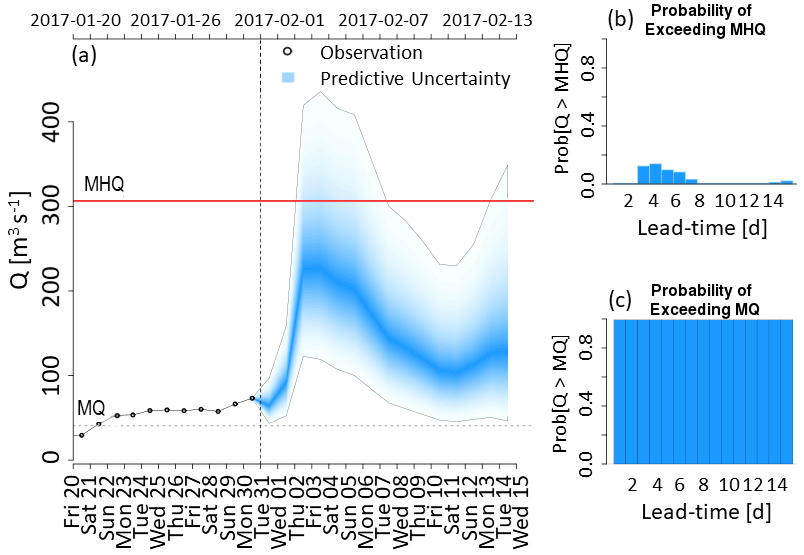
Figure 4 Example of the real-time hydrograph product for the station in Brehy, Slovakia, on 31 January 2017. (a) Probability distribution of the post-processed forecast. The darkest shade of blue indicates the forecast median (50th percentile), with each consecutive shade indicating a percentile difference such that the extent of the total predictive uncertainty is shown by the shaded region. Solid grey lines indicate the upper (99th percentile) and lower (1st percentile) bounds of the forecast probability distribution. The red line shows the mean annual maximum (MHQ) threshold, and the dashed grey line shows the mean flow (MQ) threshold. Black circles represent observations positioned at the centre of the timestep over which they are calculated. (b) Bar chart showing the probability of the discharge exceeding the MHQ threshold at each lead time. (c) Bar chart showing the probability of the discharge exceeding the MQ threshold at each lead time.

4.3.1 Forecast median

In the real-time hydrograph the darkest shade of blue indicates the forecast median, making it the easiest and most obvious single-valued summary of the full probabilistic forecast for end users. The ensemble median of the raw forecasts is used in this evaluation because operationally the ensemble forecasts are often represented by box plots where the median at each timestep is shown.

The skill of the forecast median is evaluated using the modified Kling–Gupta efficiency score (KGE', Kling et al., 2012; Gupta et al., 2009). The forecast median is determined for the post-processed forecasts by extracting the 50th percentile of the probability distribution at each lead time. For the raw forecasts the ensemble members are sorted by discharge value, and the middle (i.e. sixth) member is chosen. This is done separately for each lead time, so the overall trajectory may not follow any single member. The forecast median is denoted X to distinguish it from the full forecast, ${\mathbf{x}}_{\mathbf{t}}(t+\mathrm{1}:t+T)$. The KGE' is calculated as

$$\begin{array}{}\text{(28)}& {\mathrm{KGE}}^{\prime }=\mathrm{1}-\sqrt{(r-\mathrm{1}{)}^{\mathrm{2}}+(\mathit{\beta }-\mathrm{1}{)}^{\mathrm{2}}+(\mathit{\gamma }-\mathrm{1}{)}^{\mathrm{2}}},\end{array}$$

with

$$\begin{array}{}\text{(29)}& \mathit{\beta }={\displaystyle \frac{\stackrel{\mathrm{‾}}{X}}{\stackrel{\mathrm{‾}}{y}}}\end{array}$$

and

$$\begin{array}{}\text{(30)}& \mathit{\gamma }={\displaystyle \frac{{\mathit{\sigma }}_{\mathit{X}}/\stackrel{\mathrm{‾}}{X}}{{\mathit{\sigma }}_{\mathit{y}}/\stackrel{\mathrm{‾}}{y}}},\end{array}$$

where r is Pearson's correlation coefficient, $\stackrel{\mathrm{‾}}{X}$ and $\stackrel{\mathrm{‾}}{y}$ are the mean values of the forecast median and the observations, respectively, and σ_x and σ_y are their standard deviations. The correlation, r, measures the linear relationship between the forecast median and the observations, indicating the ability of the forecasts to describe the temporal fluctuations in the observations. The bias ratio, β, indicates whether the forecast consistently under-predicts or over-predicts the observations. The variability ratio, γ, measures how well the forecast can capture the variability of the discharge magnitude. The KGE' is calculated separately for each lead time. The KGE' ranges from −∞ to 1, r ranges from − 1 to 1, and both β and γ range from −∞ to ∞. A perfect score for the KGE' and each of the components is 1.

4.3.2 Peak discharge

The timing of the peak discharge is an important variable of flood forecasts. The peak-time error (PTE) is used to evaluate the effect of post-processing on the timing of the peak within the forecast. The PTE requires a single-valued forecast trajectory. For the reasons stated in Sect. 4.3.1, the PTE is calculated using the forecast median, X. Peaks are defined as the maximum forecast value and the PTE is calculated for forecasts where this peak exceeds the 90th percentile discharge threshold of the station. This threshold is calculated using the full observational record for the station. The PTE is calculated as

$$\begin{array}{}\text{(31)}& \mathrm{PTE}=t_n^{\mathit{X}}-t_n^{\mathit{y}},\end{array}$$

where $t_n^{\mathit{X}}$ is the timestep of the maximum of the forecast median for the nth forecast and $t_n^{\mathit{y}}$ is the timestep of the maximum observed value in the same forecast period. A perfect score is PTE = 0. A negative PTE value indicates that the peak is forecast too early and a positive PTE value indicates that the peak is forecast too late. As the maximum lead time is 15 d, the maximum value of the PTE is 14 d and the minimum value is − 14 d.

4.3.3 Threshold exceedance

Two discharge thresholds are shown in the real-time hydrograph: the mean discharge (MQ) and the mean annual maximum discharge (MHQ). Both thresholds are determined using the observations from the historic period. For the post-processed forecasts, the probability of exceedance of the MQ threshold, PoE(MQ), is calculated such that

$$\begin{array}{}\text{(32)}& \mathrm{PoE}\left(\mathrm{MQ}\right)=\mathrm{1}-F_{\stackrel{\mathrm{̃}}{\text{x}}}\left(\mathrm{MQ}\right),\end{array}$$

where $F_{\stackrel{\mathrm{̃}}{\text{x}}}\left(\mathrm{MQ}\right)$ is the value of the forecast CDF at the MQ threshold. The CDF is assumed to be linear between any two percentiles. The same method is applied for the MHQ threshold. For the ensemble forecast, each ensemble member above the threshold contributes one-eleventh to the probability of the threshold being exceeded. The probability of the threshold being exceeded is calculated separately for each lead time.

The relative operating characteristic (ROC) score and ROC diagram (Mason and Graham, 1999) are used to evaluate the potential usefulness of the forecasts with respect to these two thresholds. The ROC diagram shows the probability of detection vs. the false alarm rate for alert trigger thresholds from 0.05 to 0.95 in increments of 0.1. The ROC score is the area below this curve with a ROC score of less than 0.5, indicating a forecast with less skill than a climatological forecast. As discharge values of above the MHQ threshold are rare, all stations are combined and lead times are combined into three groups; 1–5, 6–10, and 11–15 d. Since the reforecasts are only produced on Monday and Thursdays, an event that occurs on a Saturday can only be forecasted at lead times of 2, 5, 9, and 12 d. Using 5 d groupings of lead times guarantees that each group is evaluated against each event at least once but allows the usefulness of the forecasts to be compared at different lead times. A perfect forecasting system would have a ROC score of 1.

Reliability diagrams are used to evaluate the reliability of the forecast in predicting the exceedance of the two thresholds. Reliability diagrams show the observed frequency vs. the forecast probability for bins of width 0.1 from 0.05 to 0.95. A perfectly reliable forecast would follow the one-to-one diagonal on a reliability diagram. The same combination of stations and lead times is used as with the ROC diagrams.

4.3.4 Full probability distribution

A commonly used metric to evaluate the overall performance of a probabilistic or ensemble forecast is the continuous ranked probability score (CRPS, Hersbach, 2000). The CRPS measures the difference between the CDF of the forecast and that of the observation and is defined as

$$\begin{array}{}\text{(33)}& \mathrm{CRPS}\left(F_{\stackrel{\mathrm{̃}}{x}},y\right)=\underset{-\mathrm{\infty }}{\overset{\mathrm{\infty }}{\int }}{\left(F_{\stackrel{\mathrm{̃}}{x}}\left(\stackrel{\mathrm{̃}}{\mathit{\eta }}\right)-\mathit{\theta }\left(\stackrel{\mathrm{̃}}{\mathit{\eta }}-y\right)\right)}^{\mathrm{2}}\mathrm{d}\stackrel{\mathrm{̃}}{\mathit{\eta }},\end{array}$$

where $F_{\stackrel{\mathrm{̃}}{x}}$ represents the CDF of the forecast and $\mathit{\theta }(\stackrel{\mathrm{̃}}{\mathit{\eta }}-y)$ is the step function (Abramowitz and Stegun, 1972), defined such that

$$\begin{array}{}\text{(34)}& \mathit{\theta }\left(\stackrel{\mathrm{̃}}{\mathit{\eta }}\right)=\mathit{\{}\begin{array}{cc}\mathrm{0}& \stackrel{\mathrm{̃}}{\mathit{\eta }}<\mathrm{0},\\ \mathrm{1}& \stackrel{\mathrm{̃}}{\mathit{\eta }}\ge \mathrm{0},\end{array}\end{array}$$

and represents the CDF of the observation, y. The post-processed forecasts are defined via their percentiles; therefore, by assuming the CDF is linear between percentiles, the CRPS can be calculated directly. The empirical CDF of the raw forecasts, defined via point statistics, is used and the CRPS is calculated using a computationally efficient form (Jordan et al., 2019, Eq. 3). It should be noted that the error in the calculation of the CRPS for the raw ensemble forecasts is likely to be large compared with that of the post-processed forecasts because of the limited number of ensemble members (Zamo and Naveau, 2018). However, as this evaluation is of the post-processing method, no corrections to account for the ensemble size are made (e.g. Ferro et al., 2008) since the impact of the post-processing would be difficult to differentiate from that of the CRPS correction. The CRPS ranges from a perfect score of 0 to ∞.

4.3.5 Comparison

For some of the metrics described in Sects. 4.3.1–4.3.4, the impact of post-processing is shown using the respective skill score, SS, with the raw forecast as the benchmark,

$$\begin{array}{}\text{(35)}& \mathrm{SS}={\displaystyle \frac{S_{\mathrm{pp}}-S_{\mathrm{raw}}}{S_{\mathrm{perf}}-S_{\mathrm{raw}}}},\end{array}$$

where S_pp and S_raw are the scores for the post-processed forecast and the raw forecast, respectively, and S_perf is the value of the score for a perfect forecast. The skill score gives the fraction of the gain in skill required for the raw forecast to become a perfect forecast that is provided by the post-processing. A value SS <0 means the forecast has been degraded by the post-processing, a value of SS >0 indicates that the forecast has been improved by the post-processing, and a value of SS =1 means that the post-processed forecast is perfect. Henceforth, the skill score for a metric is denoted by adding “SS” to the metric name.

5 Results and discussion

5.1 Performance of the post-processing method

This section focuses on the overall impact of post-processing at all 522 of the evaluated stations across the EFAS domain and aims to address the research question “Does the post-processing method provide improved forecasts?”

5.1.1 Forecast median

The modified Kling–Gupta efficiency skill score (KGESS) is used to evaluate the impact of post-processing on the forecast median (see Sect. 4.3.1). Figure 5a shows the KGESS for all stations at every other lead time such that each box plot (also known as letter-value plots, Hofmann et al., 2017) contains 522 values, 1 for each station. For each lead time the central black line shows the median KGESS value. The inner box (the widest box) represents the interquartile range and contains 50 % of the data points. Each subsequent layer of boxes splits the remaining data points in half such that the second layer of boxes is bounded by the 12.5th and 87.5th percentiles and contains 25 % of the data points. The outliers represent a total of 2 % of the most extreme data points. Figure 5b–d show the three components of the KGE' (b: correlation, c: bias ratio, d: variability ratio) for lead times of 3, 6, 10, and 15 d for all stations for both the raw forecasts (orange) and the post-processed forecasts (purple). The chosen lead times are representative of the results.

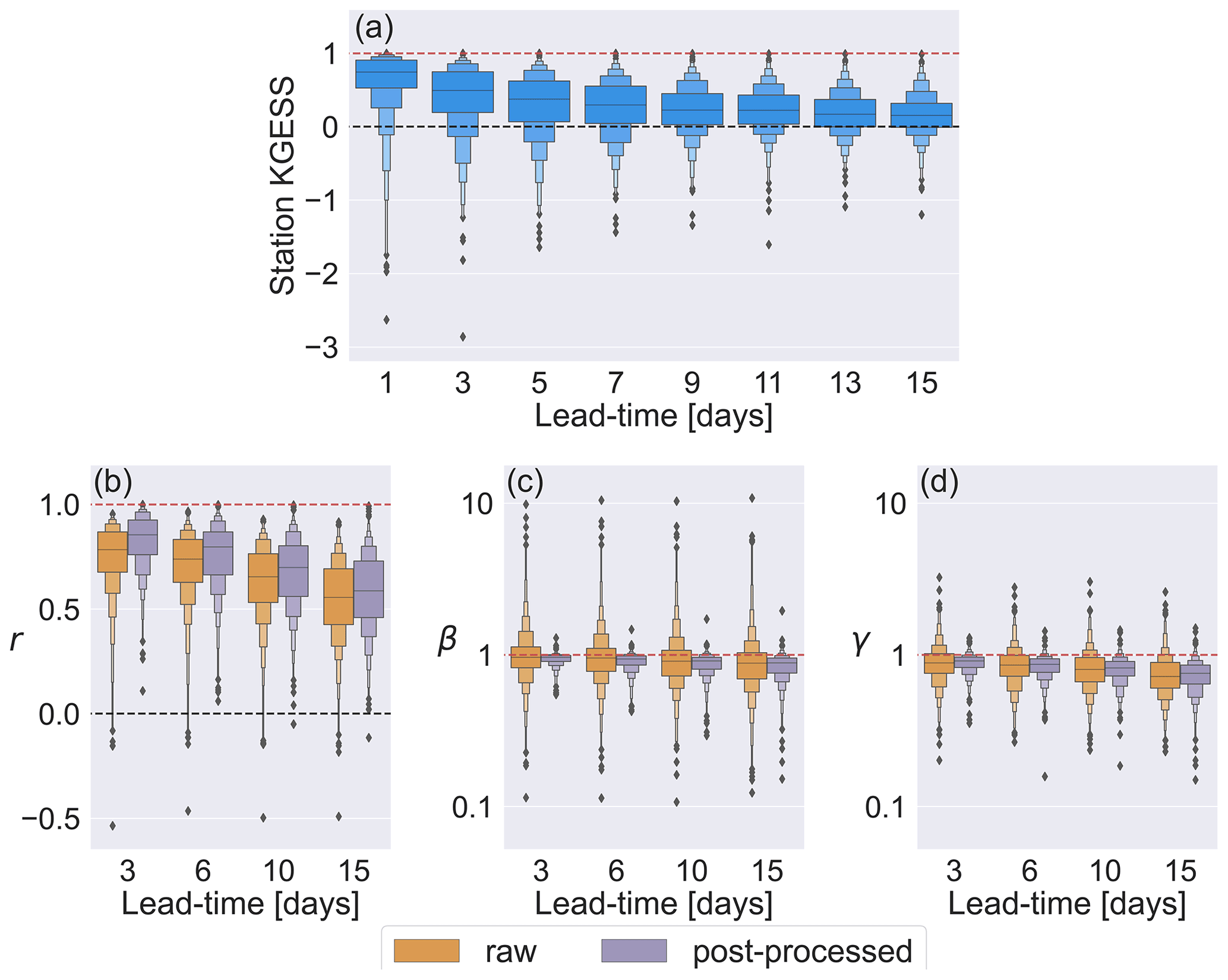
Figure 5 Comparison of the raw and post-processed forecast medians. (a) The Kling–Gupta efficiency skill score (KGESS) for the forecast medians at all 522 stations for every other lead time. Red dashed line shows the perfect score of KGESS = 1. Black dashed lines show a KGESS value of 0. KGESS > 0 indicates that the skill of the forecast median is improved by post-processing. KGESS < 0 indicates that the skill of the forecast median is degraded by post-processing. The three components of the KGE': (b) correlation component, r. Black dashed line shows r=0. (c) Bias ratio component, β. (d) Variability ratio component, γ. Red dashed lines show the perfect scores of 1 for all the components. Both panels (c) and (d) have logarithmic y axes.

Figure 5a shows that most stations have positive KGESS values at all lead times, indicating that post-processing increases the skill of the forecast median. However, the magnitude of this improvement decreases at longer lead times, with most of the reduction occurring in the first 7 d. The proportion of stations for which post-processing degrades the forecast median increases with lead time. However, the lowest KGESS values become less extreme (i.e. not as negative). This increase in the KGESS of the most degraded stations is due to a decrease at longer lead times in the skill of the raw forecast (used as the benchmark for the skill score) rather than an increase in the skill of the post-processed forecasts. This shows that the effect of naïve skill on the results should be considered; however, as the aim is to evaluate the impact of post-processing, it is appropriate to use the raw forecasts as the benchmark (Pappenberger et al., 2015b).

Figure 5b shows that post-processing improves the correlation between the forecast median and the observations for most stations, particularly at short lead times. The impact of post-processing on the correlation component of the KGE' varies greatly between stations. Notably, the flashiness of the catchment and whether or not the river is regulated can affect the performance of the post-processing (see Sect. 5.2.2). Additionally, the quality and length of the calibration time series also have an effect (see Sect. 5.2.3).

Figure 5c shows the bias ratio, β, which indicates whether on average the forecasts over-estimate or under-estimate the discharge at a station. In the hydrological uncertainty estimation part of the online correction (see Sect. 3.4.1) the mean of the hydrological uncertainty distribution is calculated in Eq. 14 as the mean flow of the observed time series from the historic period (term 1) plus an amount dependent on the discharge values in the recent period (term 2). Therefore, assuming the mean flow does not change between the calibration (historic) and evaluation periods, any consistent biases in the hydrological model climatology should be corrected.

Figure 5c shows the variability ratio, γ, which indicates whether the forecast median is able to capture the variability of the flow. In general, the post-processing method does reduce the bias in the forecast median. For raw forecasts, the β values range from approximately 10 (an over-estimation by an order of magnitude) to 0.1 (an under-estimation of an order of magnitude). For the post-processed forecasts the β values are more tightly clustered around the perfect value of β=1. The largest improvements to the β values are for stations where the flow is under-estimated by the raw forecasts. Some stations with raw β values of greater than 1 are over-corrected such that the post-processed forecasts have β values of less than 1. This is supported by the similarity of the median β values for the raw and post-processed forecasts despite the decrease in the range of values. For stations where the over-estimation by the raw forecast is relatively small, the over-correction can result in the post-processed forecasts being more biased than the raw forecasts. The over-correction is generally due to the under-estimation of high flows (see the discussion on the third component of the KGE', the variability ratio), which results in an under-estimation of the average flow and hence a β value of less than 1.

There is a small decrease in the β values at longer lead times for both the raw and post-processed forecasts. This is primarily caused by an increase in the under-estimation of high flows at longer lead times as the skill of the forecast decreases. However, for some stations the drift in β values at longer lead times is also caused by nonstationarity of the discharge distribution. A change in the discharge distribution from that of the calibration period means the hydrological uncertainty is calculated using an inaccurate climatological mean (term 1 of Eq. 14). The impact of the discharge values from the recent period (term 2 of Eq. 14) decreases with lead time because the autocorrelation weakens. Therefore, any errors in the climatological forecast are more pronounced at longer lead times.

Figure 5d shows that the variability of the flow tends to be under-estimated by the raw forecast (γ less than 1). The under-estimation is because the magnitudes of the peaks relative to the mean flow are not predicted accurately, particularly at longer lead times. This decrease in γ values at longer lead times is also visible for the post-processed forecasts. However, at all lead times most stations show an improvement after post-processing (i.e. have a value of γ closer to 1). Stations where the raw forecast over-estimates the variability (γ above 1) are more likely to have the variability corrected by post-processing, particularly at longer lead times.

The two factors impacting the ability of the post-processed forecasts to capture the variability of the flow are 1) the level of indication of the upcoming flow by the discharge values in the recent period and 2) the spread of the raw forecast. In the Kalman filter when the hydrological uncertainty distribution and the meteorological uncertainty distribution are combined (see Sect. 3.4.3), the weighting of each distribution is dependent on their relative spreads. The spread of the hydrological uncertainty is impacted by the discharge values in the recent period. Due to the skewness of discharge distributions, the climatological forecasts tend to have a low probability of high flows. If the recent discharge values show no indication of an upcoming high flow (i.e. no increase in discharge), the low probability of high flows is reinforced. This decreases the spread of the hydrological uncertainty distribution and increases its weight within the Kalman filter.

The meteorological uncertainty distribution is the spread-corrected raw forecast and includes the variability due to the meteorological forcings. For floods with meteorological drivers, if the magnitude of the peaks is under-predicted by the raw forecasts, then the post-processed forecasts are also likely to under-predict the magnitude of the peaks. Alternatively, if the raw forecast is unconfident in the prediction of a peak (e.g. only a couple of members predict a peak), then it may not have a sufficient impact within the Kalman filter and the post-processed forecast may not predict the peak regardless of the accuracy of the ensemble members that do predict the peak. The impact of the spread correction is discussed further in Sect. 5.2.1.

The ensemble mean is another commonly used single-valued summary of an ensemble forecast (Gneiting, 2011). Although the comparison presented here uses the ensemble median, we also show the three components of the KGE' for the ensemble mean in Fig. S1 in the Supplement. The ensemble means (see Fig. S1b in the Supplement) do not show the general drift in β values with increasing lead time that is discussed above for both the ensemble median and post-processed forecasts. However, the range of β values is similarly large for both the ensemble median and the ensemble mean. In terms of the correlation coefficient and the variability ratio, the ensemble mean performs similarly to or worse than the ensemble median (see Fig. S1a, c in the Supplement, respectively).

5.1.2 Timing of the peak discharge

To evaluate the impact of post-processing on the ability of the forecast to predict the timing of the peak flow accurately, the PTE (see Sect. 4.3.2) is used. The aim of this assessment is to see how well the forecast is able to identify the time within the forecast period with the highest flow and therefore greatest hazard. A PTE of less than 0 indicates that the peak is predicted too early, whereas a PTE of greater than 0 indicates that the peak was predicted too late. Figure 6 shows the distribution of the PTE values for both the post-processed and raw forecasts for all forecasts where the maximum forecast value exceeds the 90th percentile. The forecasts are split into three categories dependent on the lead time at which the forecast maximum occurs. Therefore, the distributions shown in each panel are truncated at different values of the PTE. For example, if the forecast maximum occurs at a lead time between 1 and 5 d, it can at most be predicted 5 d early.

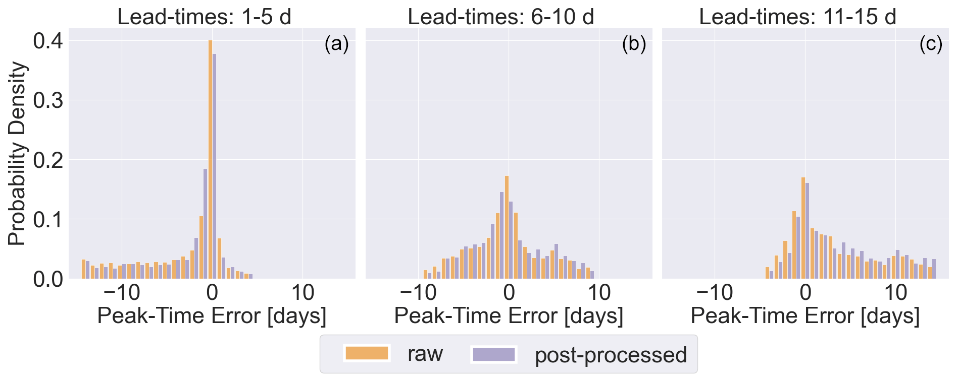
Figure 6 Histograms showing the probability distribution of peak-time errors for all forecasts where the maximum observation is above the 90th percentile for the station (26 807 forecasts) for raw forecasts (orange) and post-processed forecasts (purple). (a) Maximum observations occur at lead times of 1 to 5 d. (b) Maximum observations occur at lead times of 6 to 10 d. (c) Maximum observations occur at lead times of 10 to 15 d.

Approximately 40 % of the forecast medians of the raw forecasts have no error in the timing of the peak for peaks that occur within lead times of 1 to 5 d. This drops to 37 % for post-processed forecasts. Both sets of forecasts have approximately 60 % of forecasts with timing errors of 1 d or less. However, the post-processed forecasts are more likely to predict the peak too early. For maximum forecast values occurring at lead times of 6 to 10 d, the post-processed forecasts still tend to predict peaks earlier than the raw forecasts. However, for maximum forecast values occurring at lead times of 11 to 15 d, the post-processed forecasts are more likely to predict the peaks several days too late. This suggests that floods forecast at longer lead times by the post-processed forecasts should be considered carefully.

Overall, the impact of post-processing is small but tends towards the early prediction of the peak flow for short lead times and late peak predictions for longer lead times. However, there are three main limitations with this analysis. The first is that both sets of forecasts are probabilistic, and therefore the median may not provide an adequate summary of the forecast. Secondly, the evaluation here is forecast based rather than peak based in that the focus is the timing of the highest discharge value in the forecast within the forecast period and not the lead time at which a specific peak is predicted accurately. This was intentional, as the twice-weekly production of the reforecasts means that a specific peak does not occur at each lead time. Finally, the combination of forecasts at all the stations means the relationship between the runoff-generating mechanisms and the PTE cannot be assessed.

5.1.3 Threshold exceedance

The ROC diagrams for the MQ and MHQ thresholds (see Sect. 4.3.3) are shown in Fig. 7. The diagrams show the probability of detection against the false alarm rate for varying decision thresholds. The forecast period is split into three lead time groups: 1–5, 6–10, and 11–15 d (see Sect. 4.3.3). The ROC scores for the MQ and MHQ thresholds are given in Table 1 for each lead time group for the raw and post-processed forecasts along with the corresponding skill scores (ROCSS). Both the raw and post-processed forecasts have ROC scores greater than 0.5, showing that they are more skilful than a climatological forecast.

Figure 7 Relative operating characteristic diagrams for (a) the MQ threshold (118 888 observations above MQ) and (b) the MHQ threshold (2783 observations above MHQ). All stations are combined and groupings of lead times are used (see Sect. 4.3.3).

The spread of the raw forecasts is small at short lead times. This is shown by the overlapping of the points in Fig. 7a for lead times of 1–5 d (orange circles). The similarity of the points indicates that the decision thresholds are usually triggered simultaneously and therefore that the forecast distribution is narrow. The spread of the forecast increases with lead time as the ensemble of meteorological forcings increases the uncertainty in the forecasts. Although the skill of the forecast median decreases with lead time (see Sect. 5.1.1), the introduction of the meteorological uncertainty means the usefulness of the raw forecasts is similar for lead times of 1–5 and 6–10 d. This is shown by the similarity of the ROC scores for these lead time groups for the raw forecast.

Post-processing also accounts for the hydrological uncertainty, allowing for a more complete representation of the total predictive uncertainty. In addition, as shown in Fig. 5c, post-processing bias corrects the forecast relatively well at short lead times. The combination of spread and bias correction leads to an increase in the probability of detection for all but the highest decision thresholds and a decrease in the false alarm rate for almost all decision thresholds and lead times. The added reliability gained from post-processing decreases with lead time. The ROCSS for lead times of 1–5 d at the MQ level is 0.8 but is only 0.45 for lead times of 11–15 d.

Table 1 Relative operating characteristic scores (ROCS) and corresponding skill scores (ROCSS) for the raw and post-processed (pp) forecasts for lead times of 1–5, 6–10, and 10–15 d for the mean flow threshold (MQ) and the mean annual maximum threshold (MHQ).

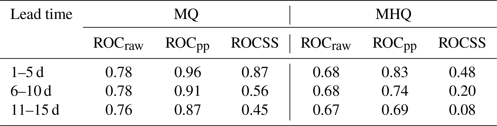
The ROC diagram for the MHQ threshold (Fig. 7b) shows that the raw forecasts tend to cautiously predict high flows, with the forecast much more likely to miss a flood than to issue a false alarm, even for the lowest decision threshold. There is less improvement from post-processing than for the MQ threshold, with the ROCSS for the MHQ threshold only reaching 0.48 for a 1–5 d lead time. For the MHQ threshold, the post-processing increases the probability of detection and decreases the false alarm rate at short lead times. At longer lead times the false alarm rate is still decreased by post-processing, but the probability of detection is also decreased for the largest decision thresholds. This reluctance to forecast larger probabilities also occurs with the MQ threshold and is due to the interaction between the hydrological and meteorological uncertainty in the Kalman filter discussed in Sect. 5.1.1.

Figure 8 shows reliability diagrams for the MQ and MHQ thresholds. For the MQ threshold (Fig. 8a), the raw forecasts are over-confident, leading to under-estimation of low probabilities and over-estimation of high probabilities. The post-processed forecasts are more reliable but also tend to under-estimate low probabilities. The raw forecasts increase in reliability with lead time, whereas the reliability of the post-processed forecasts decreases. This is also true for the MHQ threshold.

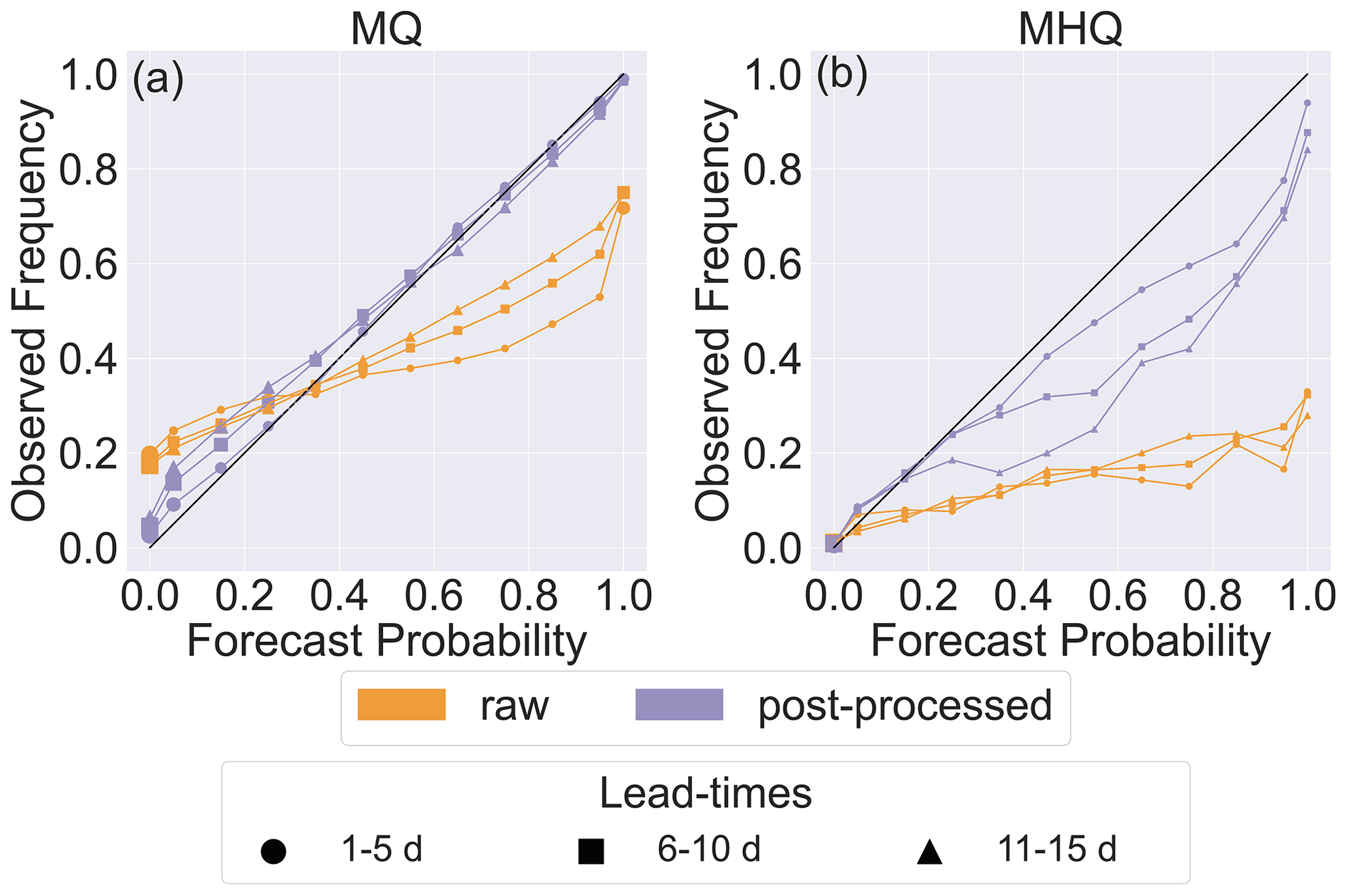
Figure 8 Reliability diagrams for (a) the MQ and (b) the MHQ. All stations are combined and groupings of lead times are used (see Sect. 4.3.3).

Both sets of forecasts are consistently below the diagonal in the MHQ reliability diagram (Fig. 8b), indicating unconditional biases. However, the post-processed forecasts have smaller biases consistent with the results discussed in Sect. 5.1.1. In addition, the raw forecast shows relatively poor resolution, with events occurring at approximately the same frequency regardless of the forecast probability.

The distribution of forecasts (shown by marker size) is more uniform for the post-processed forecasts, particularly at shorter lead times. Since the ensemble reforecasts evaluated have 11 members and the operational forecasts have 73 members, the distribution for operational raw forecasts is expected to be slightly more even as the additional members allow for greater gradation in the probability distribution. The distribution of forecasts is skewed towards low probabilities showing, similarly to the ROC diagrams (Fig. 7), that both sets of forecasts tend to cautiously forecast flows exceeding the MHQ threshold.

5.1.4 Overall skill

The continuous ranked probability skill score (CRPSS) is used to evaluate the impact of post-processing on the overall skill of the probability distribution of the forecasts. Figure 9 shows the CRPSS for each station at lead times of 3, 6, 10, and 15 d. Stations that are degraded by post-processing (CRPSS < 0) are circled in red. Stations that show a large increase in skill after post-processing (CRPSS > 0.9) are circled in cyan.

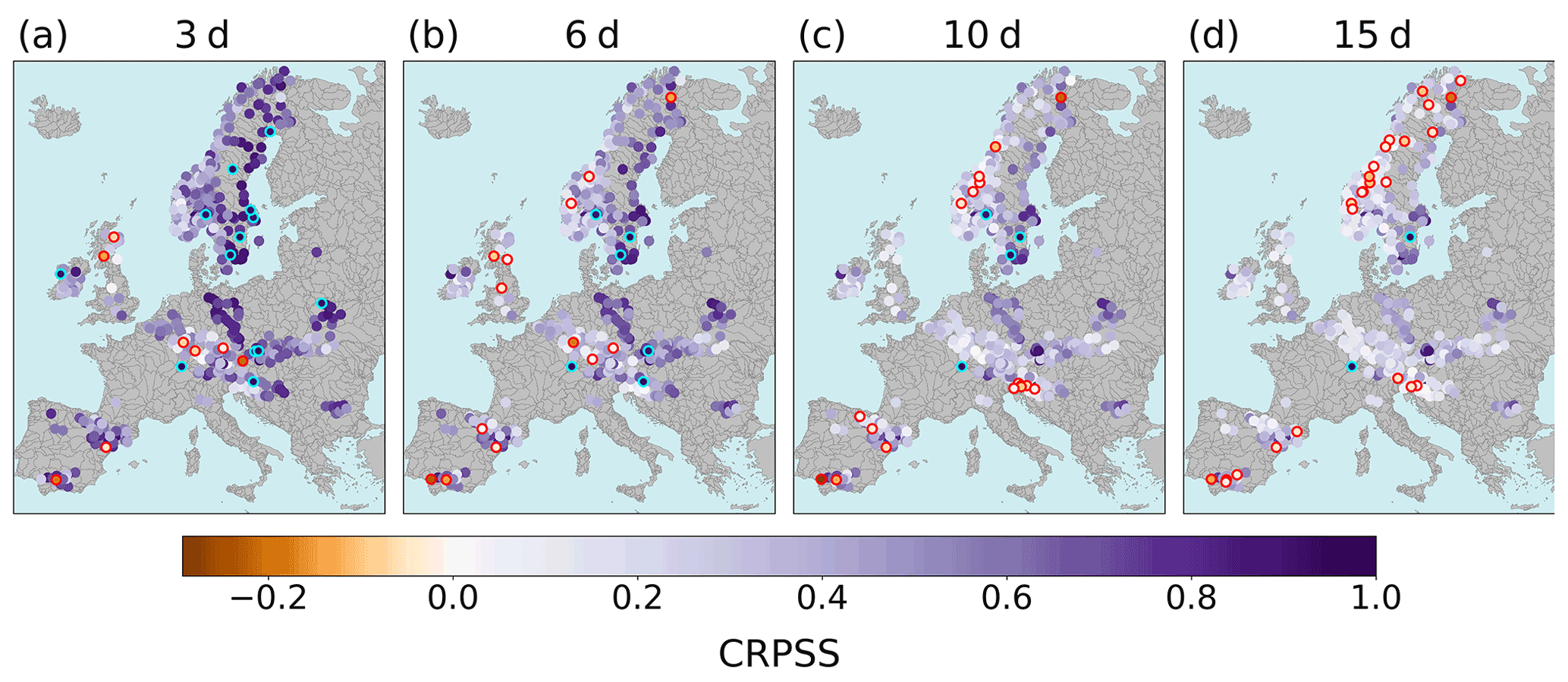
Figure 9 The continuous ranked probability skill score (CRPSS) for all 522 stations for lead times of 3, 6, 10, and 15 d. CRPSS values below 0 indicate that the forecast probability distribution is on average less skilful after post-processing and values above 0 indicate added skill after post-processing. Markers are outlined in red if the CRPSS is below 0 and in cyan if the CRPSS is above 0.9.

As was seen with the KGESS for the forecast median, there is a decrease in the improvement offered by post-processing at longer lead times. This can be seen in Fig. 9 in the gradual change from dark purple to light purple/white values for panels (a) to (d). It is also shown in the increase in red circles and the decrease in cyan circles. Approximately 55 % of stations have a CRPSS of above 0.5 at a lead time of 3 d, and this decreases to 10 % by a lead time of 15 d. At a lead time of 3 d, 8 stations are degraded by the post-processing and 13 stations have a CRPSS of greater than 0.9. By a lead time of 15 d these change to 24 degraded stations and only 2 stations with CRPSS values greater than 0.9. Many of the stations that are improved significantly have large hydrological biases. For example, one of the most improved stations at a lead time of 15 d is in Rheinweiler, Germany (see Fig. 3), which has a large bias in the hydrological model output due to limitations in the representation of the drainage network in the model domain. The post-processing method can account for these biases (see Sect. 5.1.1), resulting in CRPSS values greater than 0.9 at all lead times.

The lack of clustering of the stations with CRPSS values above 0.9 suggests that the magnitudes of the largest corrections are due to station-dependent characteristics. On the other hand, the degraded stations at a lead time of 3 d appear to cluster in three loose regions. In all three regions the degradation is due to high short-duration peaks being captured better by the raw forecasts than the post-processed forecasts. At longer lead times the Spanish catchments are still degraded, but the Scottish stations are not. As discussed in Sect. 5.1.1 for the lowest KGESS values, this is due to a decrease in the skill of the raw forecasts. The degraded stations at lead times of 10 and 15 d cluster in Spain, around the Kjølen Mountains, and in the Sava catchment. The poorly post-processed forecasts in the Sava catchment are downstream of a reservoir, the impact of which is discussed in Sect. 5.2.2.

Comparing the CRPSS values in Fig. 9 with the raw CRPS values shown in Fig. 3 shows similarities in the spatial pattern of the raw forecast skill and the spatial pattern of the magnitude of improvement due to post-processing. In general, stations with low CRPS scores (high skill) for the raw forecasts are improved most by post-processing. For example, the western coast of the Scandinavian Peninsula has a lower raw skill in general, and the level of improvement is also lower than that of the eastern coast. However, there are some anomalies to this pattern. For example, the station in Cong Weir, Ireland, has a relatively low raw forecast skill compared with surrounding catchments due to regulation of the streamflow but has a high CRPSS value at all lead times. Additionally, whilst stations on the Rhine River and the Oder River have similar raw CRPS values, the Oder River is improved more by post-processing. This suggests that post-processing is more effective at dealing with certain types of error and therefore that the benefit of post-processing is catchment dependent. This is discussed in Sect. 5.2.

As mentioned, many of the stations with CRPSS values below 0 at short lead times are degraded due to peak flows being better predicted by the raw forecasts. Therefore, the skill of the forecast at different flow levels is evaluated. Figure 10 shows the distribution of CRPSS values for all stations evaluated over the four quartiles of discharge (Q1 lower quartile to Q4 upper quartile), such that each box plot contains 522 CRPSS values, 1 for each station evaluated over approximately 52 forecasts. Only lead times of 3, 6, 10, and 15 d are shown, but these lead times are representative of the results at similar lead times.

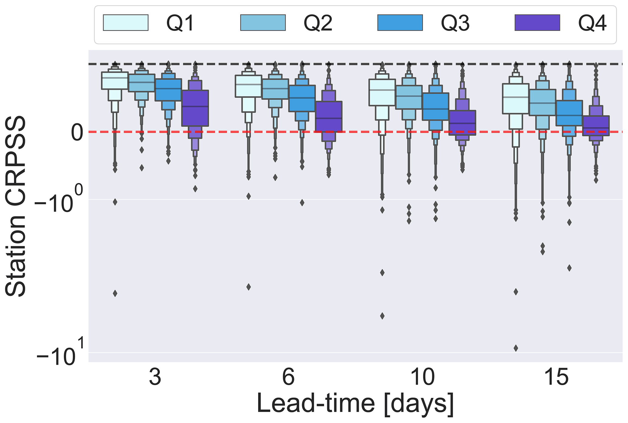
Figure 10 The CRPSS for all 522 stations calculated over the forecasts (approximately 52 forecasts) with flow values in the lowest quartile (Q1) to the highest quartile (Q4). CRPSS values below 0 indicate the forecast probability distribution is on average less skilful after post-processing and values above 0 indicate added skill after post-processing. A log scale is used on the y axis.

The improvements for all four quartiles decrease with lead time, as has been seen previously in Figs. 5 and 9. The improvement from post-processing is smaller for higher flows. However, the majority of stations are still improved for these high flows, with over 60 % of stations being improved for discharge values in Q4 at a lead time of 15 d. The high flows are often under-predicted by both sets of forecasts. As discussed in Sect. 5.1.1, the ability of the post-processed forecasts to capture the magnitude of peaks is often determined by the relative spread of the hydrological and meteorological uncertainty distributions. Although Q4 is the category with the greatest number of degraded stations (CRPSS < 0), some stations are degraded more (have a lower CRPSS value) for discharge values in Q1. This is mainly due to the larger proportional errors for lower flows.

5.2 What impacts the performance of the post-processing method?

In the previous section the impact of post-processing was shown to vary greatly between stations. The following sections investigate the factors that influence the effect of the post-processing method. The CRPSS is used in this analysis as it provides an assessment of the improvement or degradation to the overall skill of the probabilistic forecast.

To aid the discussion of the key results, some stations are highlighted. See Fig. 3 for the locations of the stations. Figure 11 shows the observed time series (solid black line) for half the evaluation period (1 October 2017 to 30 September 2018) for six example stations: (a) Daldowie, Scotland, (b) Nytorp, Sweden, (c) Svarttjørnbekken, Norway, (d) Daugavpils, Latvia, (e) Porttipahta, Finland, and (f) Montañana, Spain. The forecast medians of the raw forecasts (orange) and the post-processed forecasts (purple) are also plotted for lead times of 3 d (circles), 6 d (crosses), and 15 d (triangles). These stations are discussed throughout Sect. 5.2 and were chosen as they allow some of the impacts of the post-processing to be visualised. Table 2 summarises the key results that each of the example stations highlight, and all results are summarised in Sect. 6.

Figure 11 Observation time series for 1 year of the evaluation period from October 2017 to October 2018 for six example stations. The forecast medians of the raw and post-processed forecasts are shown for lead times of 3, 6, and 15 d. (a) Daldowie, Scotland. (b) Nytorp, Sweden. (c) Svarttjørnbekken, Norway. (d) Daugavpils, Latvia. (e) Porttipahta, Finland. (f) Montañana, Spain.

Table 2 Key results and the section that provide more information for each of the six stations used as examples and for which time series are shown in Fig. 11.

5.2.1 Type of uncertainty

This section looks at how meteorological and hydrological uncertainties affect the performance of the post-processing method. As mentioned in Sect. 1, the term “meteorological uncertainties” is used to refer to the uncertainty in the streamflow forecasts due to the error and uncertainty in the meteorological forcings and not the error in the meteorological forecasts themselves. The magnitude of meteorological uncertainty is represented here by the CRPS of the raw ensemble forecast at each lead time, respectively. To remove the uncertainty due to the hydrological model, the water balance simulation is used as the “truth” value in the calculation of the CRPS, replacing the value of the observation, y, in Eq. 33. As both the forecast and the water balance simulation are produced using the same hydrological model and the water balance simulation provides the initial conditions for the reforecasts, the only remaining uncertainty is from the forcings. The errors of the meteorological observations used to create the water balance simulation are considered negligible compared with those of the meteorological forecasts. The magnitude of the hydrological uncertainty is represented by the CRPS of the water balance simulation, with the observations used as the “truth” values at each lead time, respectively. As both these values are deterministic, the CRPS is equivalent to the absolute error between the two values. Both metrics, for the meteorological and hydrological uncertainties, are averaged over all 208 forecasts for each station. So that the errors are comparable between catchments, they are calculated in terms of specific discharge (mm d⁻¹) instead of discharge (m³ s⁻¹).

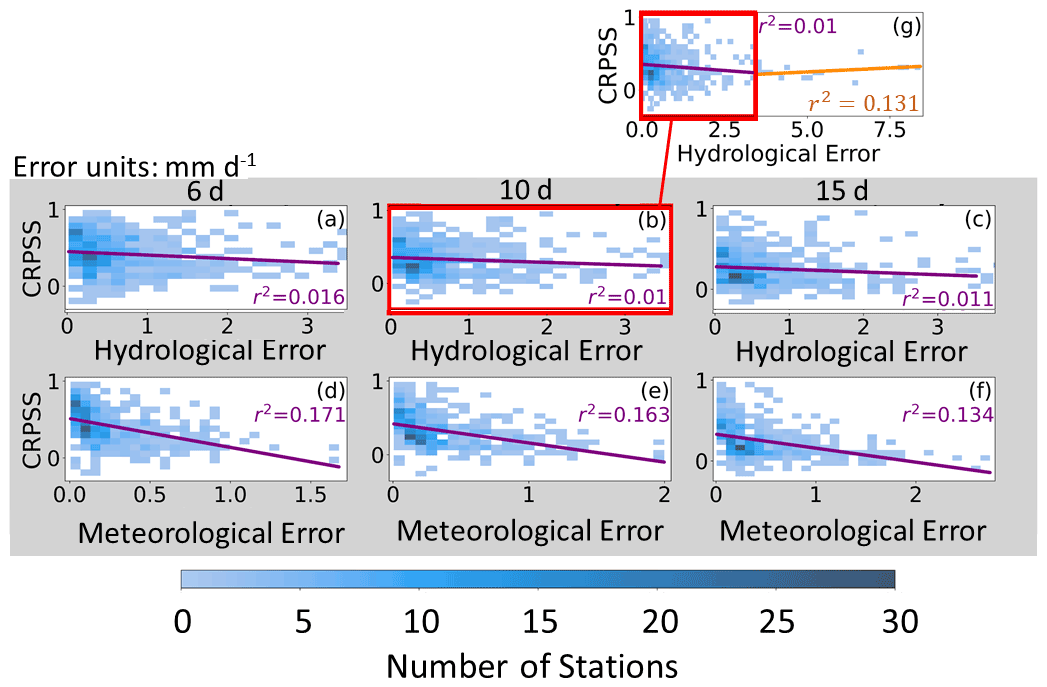
Figure 12 Density plots showing the station CRPSS for lead times of 6 d (a, d), 10 d (b, e), and 15 d (c, f) against hydrological error (a–c) and meteorological error (d–f). The largest 15 hydrological errors are excluded from panels (a) to (f). See Sect. 5.2.1 for an explanation of the metrics used to represent the hydrological and meteorological errors. Purple lines show the line of best fit calculated using linear regression, and the associated r² are given within each panel. (g) The CRPSS against hydrological error including the 15 largest hydrological errors for a lead time of 10 d. The orange line shows the line of best fit for the station with large hydrological errors.

Figure 12 shows density plots of the CRPSS values for all stations vs. the hydrological errors (a–c) and meteorological errors (d–f) for lead times of 6, 10, and 15 d. A lead time of 3 d is not shown here as the meteorological forcings have often not had a significant effect on the forecasts, resulting in a small distribution of meteorological errors across stations. However, the relationships discussed below are present at all lead times. The 15 stations with the largest hydrological errors at each lead time have been removed from the main analysis because these stations show a different pattern, as shown in Fig. 12g and discussed below.

The purple lines in Fig. 12 show the least-squares regression line of best fit for the relationship between the CRPSS vs. the hydrological and meteorological errors. In general, an increase in either the hydrological or meteorological uncertainties decreases the improvement due to post-processing. However, this relationship is much stronger for the meteorological errors (r>0.13 compared with r≈0.01 for hydrological errors), which suggests that hydrological errors are better corrected by the post-processing method. The EMOS method is used to correct the spread of the raw forecast to account for the meteorological uncertainty (see Sect. 3.4.2), but no bias correction is performed, as is sometimes done (Skøien et al., 2021; Gneiting et al., 2005; Hemri et al., 2015b; Zhong et al., 2020, e.g.), whereas both bias and spread correction are performed for the hydrological uncertainties. In Sect. 5.1.4 it was noted that the raw forecasts for the Rhine and Oder catchments have similar skill, but the Oder was improved more by post-processing. It was found (not shown) that this is because the errors in the raw forecast of the Rhine were mainly meteorological but that those of the Oder were mainly hydrological.

Although the r² values are small, some trends are observed in their variation with lead time. The relationship between the meteorological errors and the CRPSS value is slightly stronger at shorter lead times. This is partly because the EMOS spread correction parameters are lead time invariant. The spread of the raw forecast tends to be small at short lead times, because all ensemble members have the same initial conditions but increase as the differing meteorological forcings propagate through the catchment system. Skøien et al. (2021) found that the value of the variance inflation factor (ζ in Eq. 20 of this paper) decreases with increasing lead time, even becoming less than 1 (a reduction in spread) for lead times greater than 8 d (see the top left panel of Fig. 8 in Skøien et al., 2021). This alters the structure of the forecast spread, increasing the uncertainty at shorter lead times and decreasing the uncertainty at longer lead times. However, here the spread at all lead times is multiplied by a constant value such that the spread retains its original structure. Therefore, at shorter lead times the meteorological forcings are more influential within the Kalman filter than at longer lead times. On the one hand, if the raw forecast is skilled at short lead times, then this greater influence is beneficial and may, for example, allow the post-processed forecast to predict an upcoming peak. On the other hand, any large errors contained in the raw forecasts propagate through to the post-processed forecasts. For example, the largest peak in the time series for the station in Daldowie, Scotland (see Fig. 11a), is not predicted by the raw forecast; therefore, no information about the upcoming, precipitation-driven peak is provided to the post-processed forecast. Using a lead-time-dependent EMOS method may allow for better use of the information provided by meteorological forcings.

Alternatively, the hydrological uncertainty distribution may have a greater weight within the Kalman filter. Some peaks at the Daldowie station in winter 2017/2018 are forecast accurately by the raw forecast median (grey boxes in Fig. 11a) but are not forecast by the post-processed forecast. This suggests that the hydrological uncertainty distribution is most impactful in the Kalman filter. The observations in the recent period often do not indicate an upcoming flood, resulting in a hydrological uncertainty distribution which confidently, but incorrectly, predicts a low flow. The confidence of the hydrological uncertainty distribution results in the information of the upcoming flow provided by the meteorological uncertainty distribution being ignored. This ignoring of the meteorological information is also the reason for the poorly post-processed forecasts for some stations in Spain (see Fig. 9), which have very low hydrological variability except for rare large peaks. Since extreme precipitation can be an important runoff generating mechanism in this region (Berghuijs et al., 2019), post-processed forecasts for these catchments should be used cautiously, particularly when the raw forecasts predict a flood.

For the hydrological errors the r² values decrease for lead times of 1 d to approximately 6 d (not shown), and for lead times longer than 6 d, the r² values remain at approximately 0.01. This suggests that forecast-dependent errors due to the initial conditions and the interaction of the meteorological forcings in the hydrological model are corrected at shorter lead times, but at longer lead times the correction is mainly to be consistent with hydrological model errors.

The 15 stations with the largest hydrological uncertainties show a small increase in average CRPSS with increasing hydrological uncertainties. This trend is visualised by the orange line in Fig. 12g, but the limited number of data points makes the calculation irresolute. The relationship is only shown here for a lead time of 10 d but is present at all longer lead times. Most of the hydrological uncertainty in these cases is caused by large consistent biases rather than forecast-dependent errors. For example, the station in Nytorp, Sweden, has a large bias in the raw forecasts (see Fig. 11b). As discussed in Sect. 5.1.1, the post-processing method is able to correct for consistent biases, resulting in post-processed forecasts that much more closely follow the observations as shown in Fig. 11b and higher CRPSS values when the bias of the raw forecasts is larger.

5.2.2 Catchment characteristics

The catchments within the EFAS domain vary greatly in terms of size, location, and flow regime. This section discusses catchment characteristics that impact the performance of the post-processing method, namely upstream area, response time, elevation, and regulation. In Fig. 13, box-and-whisker plots are used to show the distribution of the CRPSS values for all stations at every other timestep, with the whiskers extending to the 5th and 95th percentiles. The stations are split into categories depending on (a) the size of the upstream area, (b) the time of concentration, and (c) the elevation. Values for these characteristics are extracted from static LISFLOOD maps used operationally.

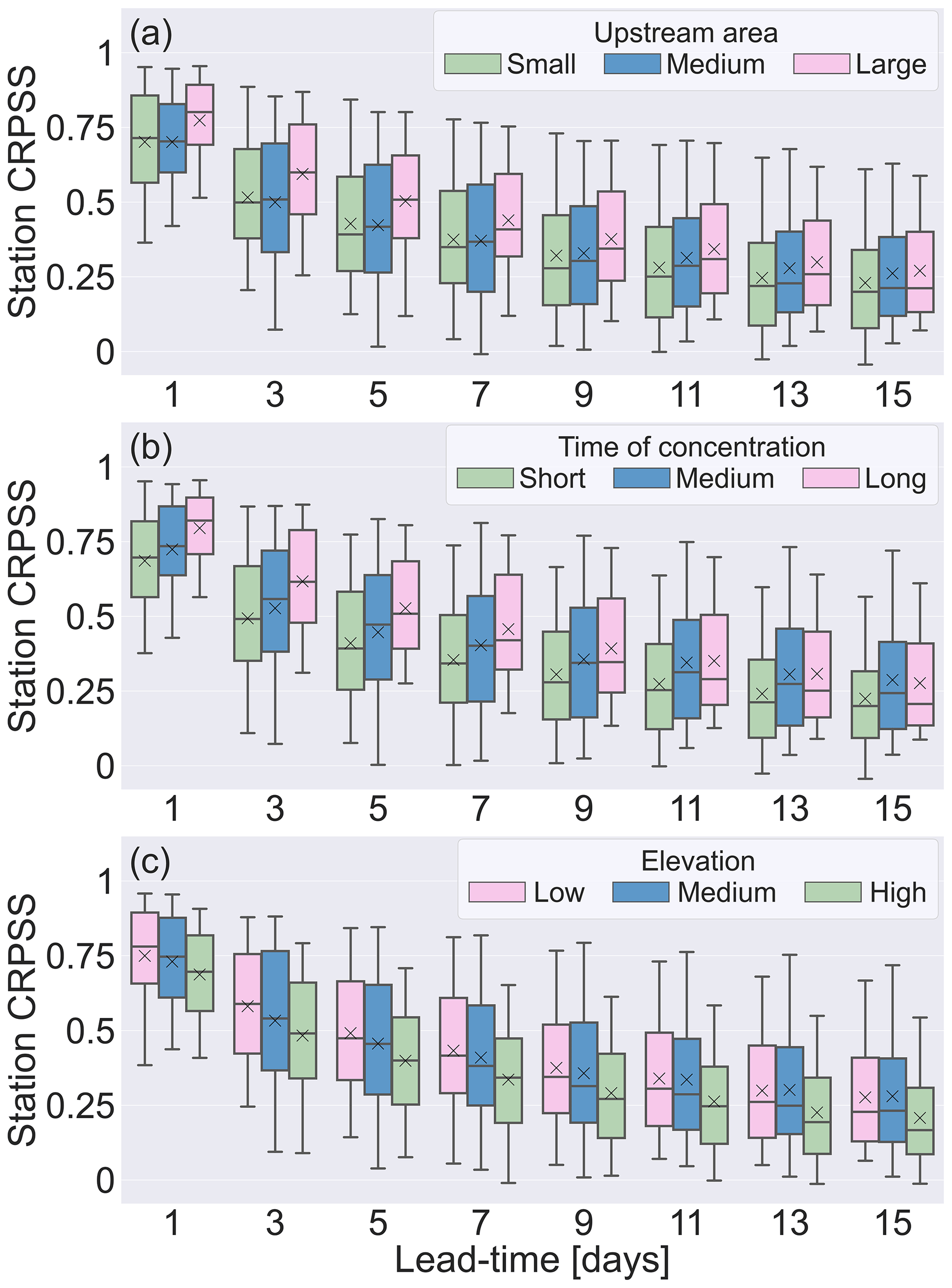
Figure 13 The CRPSS for all 522 stations at every other lead time with stations categorised by their catchment characteristics. (a) Upstream area. Small catchments: less than 1000 km² (165 stations). Medium catchments: between 1000 and 5000 km² (204 stations). Large catchments: larger than 5000 km² (153 stations). (b) Time of concentration. Fast-response catchments: less than 24 h (253 stations). Medium-response catchments: between 24 and 48 h (144 stations). Slow-response catchments: more than 48 h (126 stations). (c) Elevation. Low-elevation catchments: less than 150 m (178 stations). Medium-elevation catchments: between 150 and 400 m (168 stations). High-elevation catchments: more than 400 m (177 stations).

Figure 13a shows that, in general, large catchments (larger than 5000 km²) are improved more by post-processing than medium (between 1000 and 5000 km²) and small (less than 1000 km²) catchments, particularly at short lead times. The relationship between medium and small catchments is less consistent. At short lead times the median CRPSS value for small catchments is higher than for medium catchments, but for longer lead times the converse is true. However, it was found that by removing stations with an upstream area smaller than 500 km² (henceforth referred to as very small catchments) from the analysis, the remaining small stations (with upstream areas between 500 and 1000 km²) are in general improved less by post-processing than medium catchments at all lead times. This results in a single trend, that in general post-processing improves forecasts more for larger catchments. A partial reason for this is that smaller catchments are impacted more by spatiotemporal errors in the meteorological forcings than larger catchments (Pappenberger et al., 2011) and, as discussed in Sect. 5.2.1, meteorological errors are difficult to correct.

There are two reasons why very small catchments must be removed to clearly identify the trend between upstream area and CRPSS. Firstly, most stations with upstream areas (provided by local authorities) smaller than 500 km² were not included in the calibration of LISFLOOD for EFAS 4 (Mazzetti et al., 2021b). The uncalibrated model has varying skill between catchments, with some very small catchments having large hydrological errors. As discussed in Sect. 5.2.1, hydrological errors are well corrected by post-processing, therefore resulting in larger CRPSS values for some very small uncalibrated catchments than for larger calibrated catchments. Secondly, the minimum area increment of the LISFLOOD static map used to categorise the stations is the area of one grid box, 25 km². Therefore, the upstream areas are multiples of 25 km² and thus may not represent the real size of the catchment, which could lead to large hydrological biases. For example, the station in Svarttjørnbekken, Norway, has a catchment area provided by local authorities of 3.4 km² and was therefore not included in the calibration. Additionally, in LISFLOOD its upstream area is rounded to 25 km² (over 7 times the size of the catchment). Figure 11c shows that these issues result in an over-estimation of the variability of the flow and a consistent bias in the raw forecast even at low flows. Both issues are corrected by post-processing.

In Fig. 13b the time of concentration is used to represent the catchment response time. Stations are split into fast-response catchments (response times of less than less than 24 h), moderate-response catchments (between 24 and 48 h), and slow-response catchments (more than 48 h). At short lead times, slowly responding catchments outperform medium- and fast-response catchments. Since large catchments tend to have slower responses, this suggests response time is partly responsible for the greater improvement experienced by large catchments. Slower responses result in stronger autocorrelations; therefore, the recent observation are more informative about the state of the river during the forecast period. This is shown by comparing the time series of the Daugavpils station (Fig. 11d), which has a time of concentration of approximately 195 h, with that of the Daldowie station (Fig. 11a), which has a time of concentration of 27 h. The Daugavpils station has a slow response with peaks lasting 2 months (longer than the length of the recent period), whereas the Daldowie station responds more quickly, with peaks only lasting a week at most (shorter than the length of the forecast period). As such, the post-processing method can correct forecasts much better for the Daugavpils station. It should be noted that most stations still benefit from being post-processed even at lead times longer than their time of concentration. This is useful as operationally there is a delay in the availability of the meteorological observations used to create the water balance simulation, whereas here it is assumed that all observations up to the production time of the reforecast are available. Therefore, these results suggest that, although the CRPSS may be smaller, there is still an operational benefit to post-processing.

In Fig. 13c catchments are categorised by the height of the station above sea level: low-elevation catchments (less than 150 m), medium-elevation catchments (between 150 and 400 m), and high-elevation catchments (more than 400 m). At all lead times catchments at higher elevations are improved less than lower-lying catchments. This is partly due to mountainous catchments tending to have faster response times. Additionally, precipitation forecasts in mountainous regions can be biased due to insufficient resolutions to represent the orography in the NWP systems (Lavers et al., 2021; Haiden et al., 2014, 2021). Alfieri et al. (2014) found that, when compared with the water balance simulation (i.e. equivalent to the metric for the meteorological error used here), the raw ensemble forecasts are negatively biased in mountainous regions due to an under-estimation of the precipitation. The effect of station elevation on the performance of the post-processing method explains the cluster of degraded stations around the Kjølen Mountains (see Fig. 9).

The regulation of rivers via reservoirs and lakes is difficult to model. Raw forecasts for many regulated catchments were found to have a negative correlation with the observations. In this study, a station is considered to be regulated if it is within three grid boxes downstream of a reservoir or lake in the LISFLOOD domain or if data providers have reported that the station is on a regulated stretch of the river. Figure 14 shows the CRPSS values of the 42 regulated stations (black lines) and the distribution of the CRPSS values of the unregulated stations (green distribution) for lead times of 3, 6, 10, and 15 d. The distribution for the unregulated stations is estimated using kernel density estimation, with the dashed line showing the median value and the dotted lines showing the interquartile range. The mean CRPSS values are indicated by crosses of the respective colours.

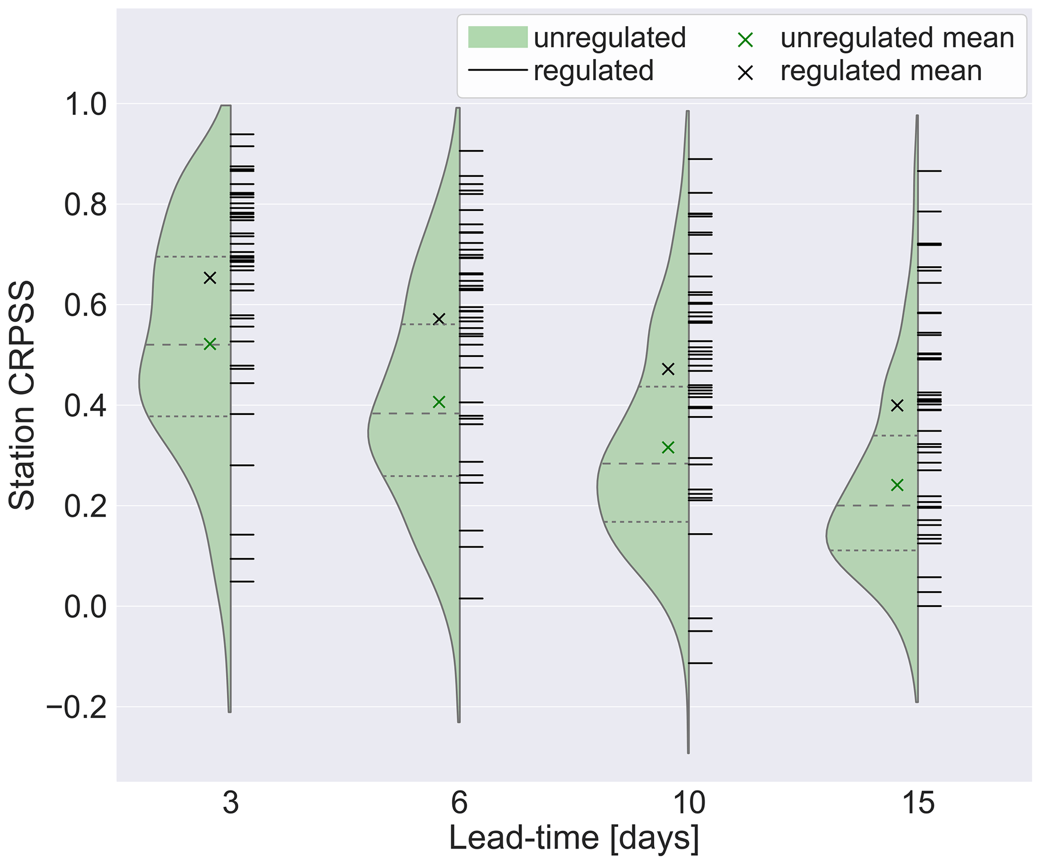
Figure 14 Violin plot of the CPRSS values for the 480 unregulated stations (green distribution) and the 42 regulated catchments (black lines) at lead times of 3, 6, 10, and 15 d.

At all lead times, the CRPSS values of most regulated stations are above the median of the unregulated stations. Additionally, the mean CRPSS value of the regulated stations is at least 0.1 higher than that of the unregulated stations for all lead times longer than 1 d. The improvement due to post-processing at regulated stations is dependent on whether the reservoir is in the same state during the recent and forecast periods and hence whether the discharge values from the recent period provide useful information about the state of the reservoir. At longer lead times it becomes more likely that the reservoir will have a changed state and therefore that the information provided by the recent discharge values is not useful. However, if the reservoir is in the same state, then the magnitude of the improvement from post-processing can be large. For example, the Porttipahta station in Finland is located at the Porttipahta reservoir, and its time series is shown in Fig. 11e. In May 2018 the discharge is 0 m³ s⁻¹ for approximately a month. The raw forecast does not capture this decrease in discharge, but the post-processed forecast median is very accurate even at longer lead times. However, at the start and end of this zero-flow period, the post-processed forecasts do not perform as well for a lead time of 15 d (purple triangles) because the reservoir has changed state since the forecast production time. It is thought that small but regular regulation is partly responsible for the cluster of degraded stations on the Sava River shown for a lead time of 10 d in Fig. 9c. Three of the degraded stations in this cluster are regulated and are the three regulated stations with the lowest CRPSS values at all lead times shown in Fig. 14.

It is interesting to consider whether other hydrological processes that are difficult to model can be accounted for by post-processing. For example, the peak in the winter and spring in the Daugavpils catchment (see Fig. 11d) is largely dominated by snowmelt and ice melt (Škute et al., 2008), which are difficult processes to model (Alfieri et al., 2014). Figure 11d shows that the raw forecasts do not predict the magnitude of the peak in late January, but the post-processed forecasts, which are conditioned on recent observations that indicate the increase in discharge due to snowmelt, do accurately predict the peak. Similar results were seen in other catchments with snow-dominated regimes. Although the identification of dominating runoff-generating mechanisms for all catchments and seasons is beyond the scope of this study, the results presented in this section suggest that post-processing can correct for errors introduced by the imperfect modelling of slow hydrological processes.

5.2.3 Calibration time series

The length of the time series used to calibrate the station model varies between stations. The maximum length is dictated by the water balance simulation, which is available from 1 January 1990. However, many stations have shorter time series due to the availability of observations. Figure 15 shows the CRPSS values for each lead time, with stations split by the length of their calibration time series into unequally sized categories (see caption): very short time series (up to 15 years), short time series (between 15 and 20 years), medium time series (between 20 and 25 years), and long time series (over 25 years). These categories were chosen to investigate the impact of the length of the calibration time series whilst keeping the number of stations in each category as large as possible. These initial comments ignore the very short time series (green) which are discussed in more detail below.

At short lead times long time series in general lead to more improvement by post-processing than shorter time series. Longer time series allow the joint distribution between the observations and the water balance simulation to be more rigorously defined, allowing a more accurate conditioning of the forecast on the discharge values from the recent period. For lead times greater than 7 d the CRPSS distributions for all categories are similar. As discussed in Sect. 5.2.1, post-processing corrects forecast-specific errors at short lead times, but at longer lead times it is mainly consistent errors in the climatology that are corrected. The similarity of the CRPSS distributions suggests that short time series are sufficient to capture these consistent errors. This is also shown by the relatively good performance of stations with very short time series. Although a full sensitivity analysis is beyond the scope of this study, these results suggest that very short time series can be used, if necessary, to correct for consistent biases, although longer time series are preferable. However, care should be taken when forecasting high flows since a short time series will not allow for a robust calculation of the upper tail of the discharge distribution (see Sect. 3.3.1), which will likely cause errors in the forecast probability distribution (Bogner et al., 2012).

Figure 15 The CRPSS for all 522 stations at every other lead time with stations categorised by the length of their calibration time series. Very short time series: less than 15 years (63 stations). Short time series: 15 to 20 years (93 stations). Medium time series: 20 to 25 years (119 stations). Long time series: over 25 years (247).

In general, shorter time series tend to be more recent and so benefit from improved river gauging technology and also because non-stationarity between the calibration and evaluation periods is less likely to be an issue. The station in Montañana (shown in Fig. 11f) is an example of a station where a period of poor-quality observations in the calibration time series impacts the calibration, resulting in a large jump in the CDF of the observed discharge distribution as highlighted by a red circle in Fig. 16b. This CDF is used in the NQT, and the large jump results in non-smooth forecast probability distributions. Additionally, these errors were found to impact the estimation of the joint distribution, which resulted in a decrease in the correlation coefficient after post-processing. Removing the erroneous observations improved the discharge estimations, suggesting that the priority should be to use the best-quality data available even if the resultant calibration time series is shorter.

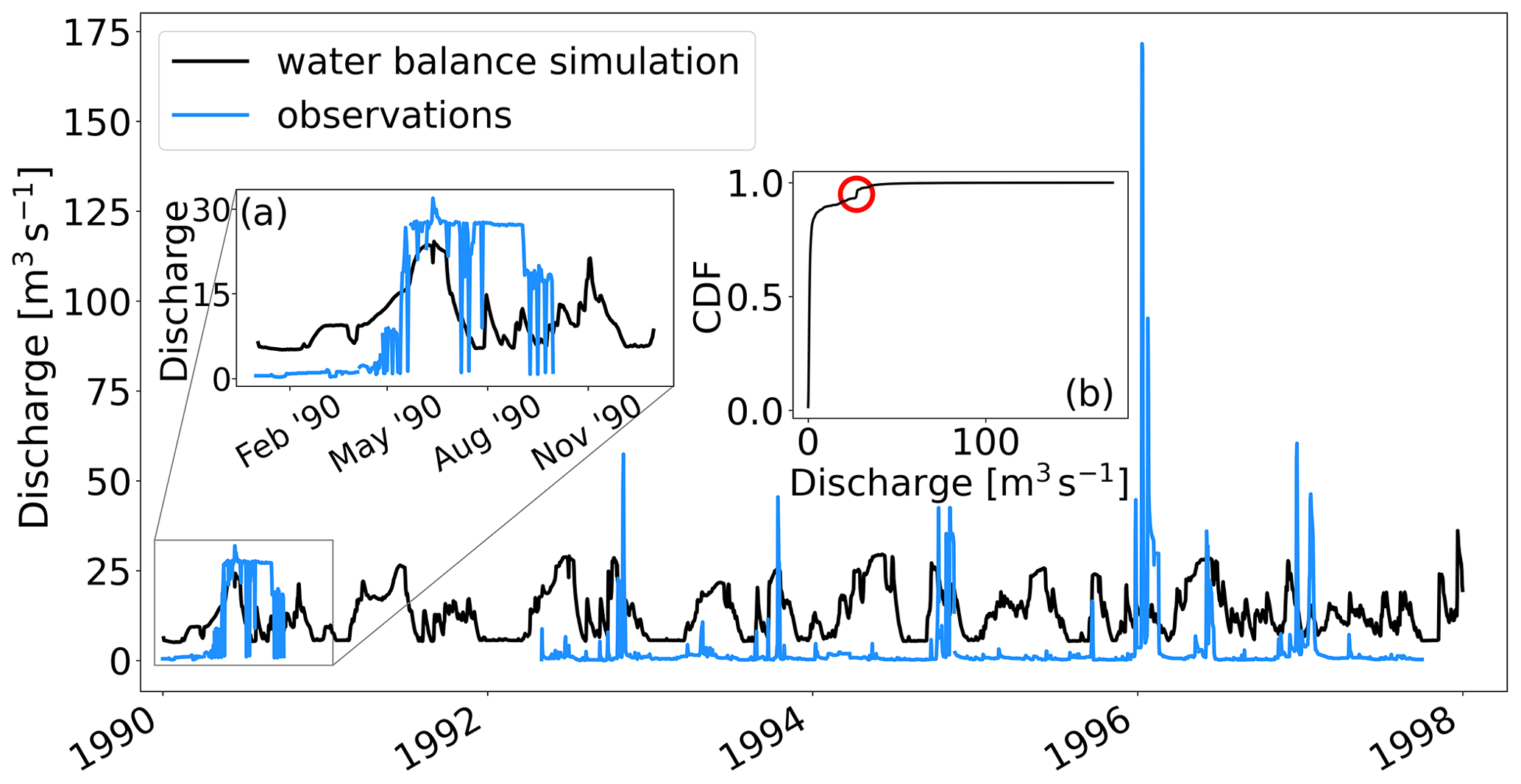
Figure 16 Observations (blue) and water balance simulation (black) time series used in the calibration of the station model for the station in Montañana. (a) Section of the calibration time series with errors in the observations. (b) The cumulative distribution function (CDF) of the observed discharge distribution calculated during the calibration. Red circle indicates a jump in the CDF due to the section of the time series shown in panel (a).

6 Conclusions

Post-processing is a computationally efficient method of quantifying uncertainty and correcting errors in streamflow forecasts. Uncertainties enter the system from multiple sources, including the meteorological forcings from numerical weather prediction systems (here referred to as meteorological uncertainties) and the initial hydrological conditions and hydrological model (here referred to as hydrological uncertainties). The post-processing method used operationally in the European Flood Awareness System (EFAS) uses a method motivated by the ensemble model output statistics (Gneiting et al., 2005) method to account for the meteorological uncertainty and the Multi-Temporal Model Conditional Processor (Coccia, 2011) to account for the hydrological uncertainty. The EFAS domain includes catchments of varying characteristics for which the same post-processing method is used. In this paper we used reforecasts to investigate the added skill gained by post-processing and how these improvements vary across the domain. This study aimed to answer two research questions.

First, does the post-processing method provide improved forecasts? Our results show that for the majority of stations the post-processing improves the skill of the forecast, with median continuous ranked probability skill scores (CRPSS) of between 0.74 and 0.2 at all lead times. This improvement is greatest at shorter lead times of up to 5 d, but post-processing is still beneficial up to the maximum lead time of 15 d. The bias and spread correction provided by the post-processing increased the reliability of the forecasts and increased the number of correctly forecast flood events without increasing the number of false alarms. However, the post-processed forecasts also led to the flood peak often being forecast too early by approximately a day. Although forecasts for flood events at most stations did benefit from post-processing, the greatest improvements were to forecasts for normal flow conditions.

Second, what affects the performance of the post-processing method? Several factors were found to impact the performance of the post-processing method at a station. The post-processing method is more easily able to correct hydrological errors than meteorological errors. This is mainly because no bias correction is performed for the meteorological errors, whereas hydrological errors are bias corrected by conditioning the forecast on the recent observations. Therefore, stations where the errors were primarily due to hydrological errors were improved more. As the hydrological errors tend to be larger than the meteorological errors, this is beneficial; however, more research is required to fully account for biases due to the meteorological forcings as well.

The post-processing method was found to easily account for consistent hydrological biases that were often due to limitations in the model representation of the drainage network. However, the correction of forecast-specific errors (due to initial conditions and meteorological forcings) was largely determined by the response time of the catchment. Therefore, the greatest improvement was seen in catchments larger than 5000 km² and catchments less than 100 m above sea level, as these catchments tended to have longer response times. Additionally, post-processing was able to correct for errors due to difficult-to-model hydrological processes, such as regulation and snowmelt, when recent observations contained relevant information about the discharge.

The use of long historic observational time series for the offline calibration is beneficial, particularly for correcting forecast-specific errors. However, time series shorter than 15 years were found to be sufficient for correcting consistent errors in the model climatology even at a lead time of 15 d. The quality of the observations in the historic time series is important, and errors in the time series degraded the performance of the post-processing method and limit the usefulness of the forecasts.

These results highlight the importance of post-processing within the forecasting chain of large-scale flood forecasting systems. They also provide a benchmark for end users of the EFAS forecasts and show the situations when the post-processed forecasts can provide more accurate information than the raw forecasts. These results also highlight possible areas of improvement within the EFAS and the factors that must be considered when designing and implementing a post-processing method for large-scale forecasting systems.