Influences of land use changes on the dynamics of water quantity and quality in the German lowland catchment of the Stör

Understanding the impacts of land use changes (LUCCs) on the dynamics of water quantity and quality is necessary for the identification of mitigation measures favorable for sustainable watershed management. Lowland catchments are characterized by a strong interaction of streamflow and near-surface groundwater that intensifies the risk of nutrient pollution. In this study, we investigated the effects of long-term changes in individual land use classes on the water and nutrient balance in the lowland catchment of the upper Stör in northern Germany. To this end, the hydrological model SWAT (Soil and Water Assessment Tool) and partial least squares regression (PLSR) were used. The SWAT model runs for three different land use maps (1987, 2010, and 2019) were conducted, and the outputs were compared to derive changes in water quantity (i.e., evapotranspiration – ET; surface runoff – SQ; base flow – BF; water yield – WYLD) and quality variables (i.e., sediment yield – SED; load of total phosphorus – TP; load of total nitrogen – TN). These changes were related to land use changes at the subbasin scale using PLSR. The major land use changes that significantly affected water quantity and quality variables were related to a decrease in arable land and a respective increase in pasture and urban land during the period of 1987–2019. Changes in landscape indictors such as area size, shape, dominance, and aggregation of each land use class accounted for as much as 61 %–88 % (75 % on average) of the respective variations in water quantity and quality variables. The aggregation, contiguity degrees, and area extent of arable land were found to be most important for controlling the variations in most water quantity variables. Increases in arable (PLAND_a) and urban land percent (PLAND_u) led to more TP and TN pollution, sediment export, and surface runoff. The cause–effect results of this study can provide a quantitative basis for targeting the most influential change in landscape composition and configuration to mitigate adverse impacts on water quality in the future.

1 Introduction

Good water quality and quantity are essential for enhancing ecological stability and diversity, and both play important roles in maintaining sustainable agricultural or economic development and human health (Lu et al., 2015; Singh et al., 2017; Antolini et al., 2020; Gleick, 2000; Srinivasan and Reddy, 2009). The water resources dynamics within a catchment are mainly governed by a combination of climate and land use, as other catchment characteristics (e.g., topography, soil, and lithology) usually do not change in the short term (Shuster et al., 2005; Farjad et al., 2017; Wagner et al., 2018). Conversely, hydrology affects land use as well (Wagner and Fohrer, 2019; Wagner and Waske, 2016). In the past 3 decades, land use changes with respect to urbanization, deforestation, and agriculture intensification have exerted significant effects on water quality or water balance components (Wagner et al., 2016; Shrestha et al., 2018; Kändler et al., 2017). They can alter surface roughness, evapotranspiration, soil infiltration, and the interaction between surface and subsurface water (Fiener et al., 2011; Wei et al., 2007; Lei et al., 2021), and promote or hinder the generation and transportation of soil particles, chemicals, or metals (Nafi'Shehab et al., 2021; Taka et al., 2022; Ding et al., 2016). Given the direct and indirect effects of land use changes on hydrological processes and contaminant inputs, it is of great practical significance to identify key predictor variables to achieve an effective catchment management of land and water resources.

Earlier studies have often aimed at analyzing land use change effects using lumped indicators of landscape composition, e.g., areal percentage of a land use class in the catchment (Kumar et al., 2022; Lei et al., 2021). However, composition indicators do not convey any details with respect to the spatial settings of landscape patterns. The configuration of the spatial land use distribution is another fundamental element measured using landscape metrics (i.e., metrics to quantify the spatial structure of land use patterns within a defined geographic area). Compared to the composition indicators that refer to the abundance (e.g., areal percent) of land patches (i.e., homogenous areas of the landscape; Hesselbarth et al., 2019) belonging to one certain class without considering their spatial characteristics, landscape configuration metrics describe spatial fragmentation or distribution of patches, e.g., the shape complexity. Landscape configuration metrics of the dominance, diversity, shape, aggregation, and interconnection of land patches play a critical part in determining the energy and matter fluxes of, e.g., solar radiation, temperature, evapotranspiration, surface runoff, nutrients, and sediments from the landscape ecology perspective (Forman, 1995; Wu and Lu, 2021; Lei et al., 2019; Amiri and Nakane, 2009). They were found to be more important as descriptors of water quality than composition indicators in some case studies. For example, Ding et al. (2016) observed that poorer water quality was not as much associated with areal percentage as with higher patch densities (PDs) of cropland, orchards, and grassland, and a higher value of the largest patch index (LPI) of urban land, in a low-order stream-dominated catchment (drainage area of 35 340 km²) in southeastern China. Despite little consideration of the landscape configuration in the studies of water quantity (Shrestha et al., 2018; Anand et al., 2018), the shape, dominance, or connectivity degree of the land patches is closely linked to the modification of the hydrological cycle. For example, more fragmented forest patches may favor the funneling of precipitation (Ghimire et al., 2017); the hardness and straightness of land patches of farmland, urban, and natural land uses influence the streamflow rates at different magnitudes and directions (Riitters, 2019; Shi et al., 2013); more concentrated grassland patches result in greater evapotranspiration (Yu et al., 2020). Therefore, it is necessary to assess the influences of changes in different aspects of a land use class to better understand their impacts on water resources dynamics.

To quantify the effects of land use changes on water resources, hydrological models are widely used (Gabriels et al., 2021; Idrissou et al., 2022; Wijesekara et al., 2012), e.g., SWAT (Soil and Water Assessment Tool; Arnold et al., 1998), HSPF (Hydrological Simulation Program–FORTRAN; Bicknell et al., 2001), or DHSVM (Distributed Hydrology Soil Vegetation Model; Wigmosta et al., 1994). Models are particularly useful for detecting historic and future land use change impacts by applying a scenario analysis (Aredo et al., 2021; Anand et al., 2018). As a physically based and semi-distributed hydrological model, SWAT has proven its suitability for an integrated modeling of water, sediment, and nutrient dynamics in different-sized rural catchments (Aghsaei et al., 2020; Tan et al., 2021). SWAT has been applied in many catchments worldwide to investigate the hydrological and hydrochemical effects (Amin et al., 2020; Boongaling et al., 2018; Anand et al., 2018). In lowland areas, the transport of water and nutrients is strongly influenced by flat topography and shallow groundwater tables in addition to the spatially heterogonous land use. The hydrological model SWAT has proven its suitability in modeling the ecohydrological consequences of spatiotemporal land use changes in lowland catchments (Guse et al., 2014; Pott and Fohrer, 2017b). Particularly in several lowland catchments in northern Germany, SWAT was extensively tested in impact studies. For example, Lam et al. (2012) modeled the long-term observations of daily streamflow and nitrate load in the Kielstau catchment and found that diffuse source pollution (dominated by agriculture) contributed dominantly (95 %) to nitrate load. In the Upper Stör catchment, Song et al. (2015) coupled SWAT with HEC-RAS (Hydrologic Engineering Center River Analysis System) to analyze the temporal dynamics of sediment loads in subbasins covered by heterogonous land use conditions. Despite a high feasibility of SWAT modeling water quantity and quality, previous studies illustrated that the original SWAT version sometimes performed relatively poorly for recession limbs and low flow periods of streamflow (Guse et al., 2014; Pfannerstill et al., 2014). In lowland catchments, the groundwater contributes significantly to low flows and, thus, becomes a dominant component of streamflow (Pott and Fohrer, 2017b). To more accurately model low flows, an enhanced version of SWAT, SWAT_3S, was developed in the Kielstau catchment, by conceptually separating the shallow groundwater aquifer of the original SWAT into a fast and slow shallow aquifer (Pfannerstill et al., 2014). SWAT_3S was successfully used for modeling daily streamflow and nitrogen loads in a few German lowland catchments (e.g., Kielstau and Treene) by improving the representation of low flow periods (Pfannerstill et al., 2014; Haas et al., 2017). Given the aforementioned strength, SWAT_3S is suitable for assessing the impacts of land use changes on water resources in lowland areas dominated by groundwater recharge.

While the changes in landscape composition and configuration have a great potential to influence hydrology, soil erosion, or water quality dynamics at different spatial and seasonal scales (Jones et al., 2001; Kändler et al., 2017; Haidary et al., 2013), some landscape metrics may have a high probability for collinearity. The collinear landscape metrics carry redundant information and are not independent predictor variables (Hargis et al., 1998). They can, therefore, result in biased or even misleading results when using conventional multivariate regression techniques like ordinary least square regression, particularly in the case of a small number of observations (Shi et al., 2013; Shawul et al., 2019). Compared to ordinary multivariate statistical methods, partial least squares regression analysis (PLSR) can overcome the limitation of multicollinearity and achieve a robust performance by using techniques of multivariate statistical projection (Shi et al., 2013). Based on the powerful technique of projecting predicted and observed variables onto a new space and estimating the underlying structure between projected spaces, PLSR facilitates an unbiased analysis of cause-+effect relationships between land use changes and water resources components (Shi et al., 2013; Yan et al., 2013; Ferreira et al., 2017). Using an integrated approach of PLSR and hydrological modeling with SWAT, impacts of the land use changes on various water resources components can be effectively identified. For example, in the Upper Du catchment, China, Yan et al. (2013) observed that the farmland positively influenced streamflow and sediment yield, whereas forest area showed a negative correlation with them; besides, urban expansion would cause streamflow to increase as well. Shi et. al. (2013) indicated that the landscape metrics e.g., Shannon's diversity index (SHDI), the aggregation index (AI), the largest patch index (LPI), contagion (CONTAG), and the patch cohesion index (COHESION) were important for controlling soil erosion and sediment yield, contributing 65 % and 74 % to their variations at subbasin level, respectively. Gashaw et al. (2018) anticipated that more shrubland would cause water yield and surface runoff to decrease, while causing evapotranspiration and groundwater flow to rise; however, increased cultivated land would result in decreases in groundwater flow and evapotranspiration in Blue Nile basin, Ethiopia. In summary, it has been demonstrated that PLSR is efficient for distinguishing the complex impacts on water quantity and quality.

The Stör river is the longest tributary of the Elbe river in the northernmost federal state of Germany, Schleswig-Holstein. Intensive agricultural activities (e.g., grazing, tillage, fertilizer, and pesticide application) are common in the catchment and increase the risk of water quality pollution (Monaghan et al., 2007). A variety of amelioration measures, e.g., tile drainage and straightening or canalizing of tributaries, have been implemented in the past century to sustain agriculture productivity in lowland areas dominated by shallow groundwater tables and abundant groundwater recharge. These activities have brought about changes in the input and transport of nutrients and in hydrological fluxes. Meanwhile, the heterogeneity of the landscape pattern has been intensified due to artificial disturbances (Gu et al., 2007; Goldewijk and Ramankutty, 2004). We previously found significant relationships between land use patterns and water quality parameters at the landscape level in the upper Stör catchment based on measurements (Lei et al., 2021). A modeling approach allows the modeling of the quantitative contribution of land use changes on water quality and quantity and facilitates the development of informed and practicable strategies for sustainable land and water management (Ripl et al., 1996; Pott, 2014).

To identify the key land use changes controlling the spatial and temporal variations in water quantity and quality, relationships between landscape characteristics of each land use class and water quality (represented by sediment, total phosphorus, TP, and total nitrogen, TN) and quantity (represented by evapotranspiration, surface runoff, base flow, and water yield) were explored at the subbasin scale in the upper Stör catchment. To this end, the hydrological model SWAT and partial least squares regression (PLSR) were employed. The study aims at (1) calibrating and validating a catchment model for streamflow, sediment, TP, and TN loads, (2) quantifying the changes in landscape characteristics and water quality and quantity variables at the subbasin scale, (3) investigating the relationships (depicted by the contribution and influence) between land use change (LUCC) and water quality and quantity dynamics at the subbasin scale.

2 Materials and methods

2.1 Study area

The rural lowland catchment of the Upper Stör is the focus of this study (Fig. 1). It extends from the origin of the Stör river in Willingrade to the gauge in Willenscharen (Fig. 1) and is free of tidal influence. The catchment has a drainage area of approximately 462 km², with a total length of the river network of about 221 km. Its temperate climate is characterized by an average annual precipitation of 850 mm and a mean temperature of 9.4 ^∘C between 1990 and 2019, according to the records by the weather stations of Neumünster and Padenstedt (DWD, 2020b). The average daily streamflow measured at the catchment outlet in Willenscharen was 5.8 m³ s⁻¹ between 1990 and 2019, with low flows (mean value of 3.8 m³ s⁻¹) in summer (May–October) and high flows (mean value of 7.9 m³ s⁻¹) in the winter (November–April) months (LKN, 2020a). Discharge occurring in the highest flow period (December–March) contributes most (around 50 %) to the total annual amount of streamflow. The catchment is characterized by a flat topography, descending from nearly 60 m a.s.l. in the northeast and 85 m in the western part, towards 20 m in the center and to 5–10 m in the southern part. Sandy soil (Cambisol, Gley-Podsol, and Podsol) dominates the catchment, particularly in the central lowland part, while some Gley soils are mainly distributed in the east, and peat soils can be found in proximity to streams and near two major wetlands (Pott and Fohrer, 2017a). The catchment is dominated by rural land use composed of arable land (36.1 %) and pasture (31.3 %), followed by forest (18.7 %), urban areas (12.8 %), and a minor fraction of water and wetland, as indicated by a land use map for 2019 (Lei et al., 2021). The main cultivated crops include winter cereals (wheat, barley, and rye), corn, and rapeseed.

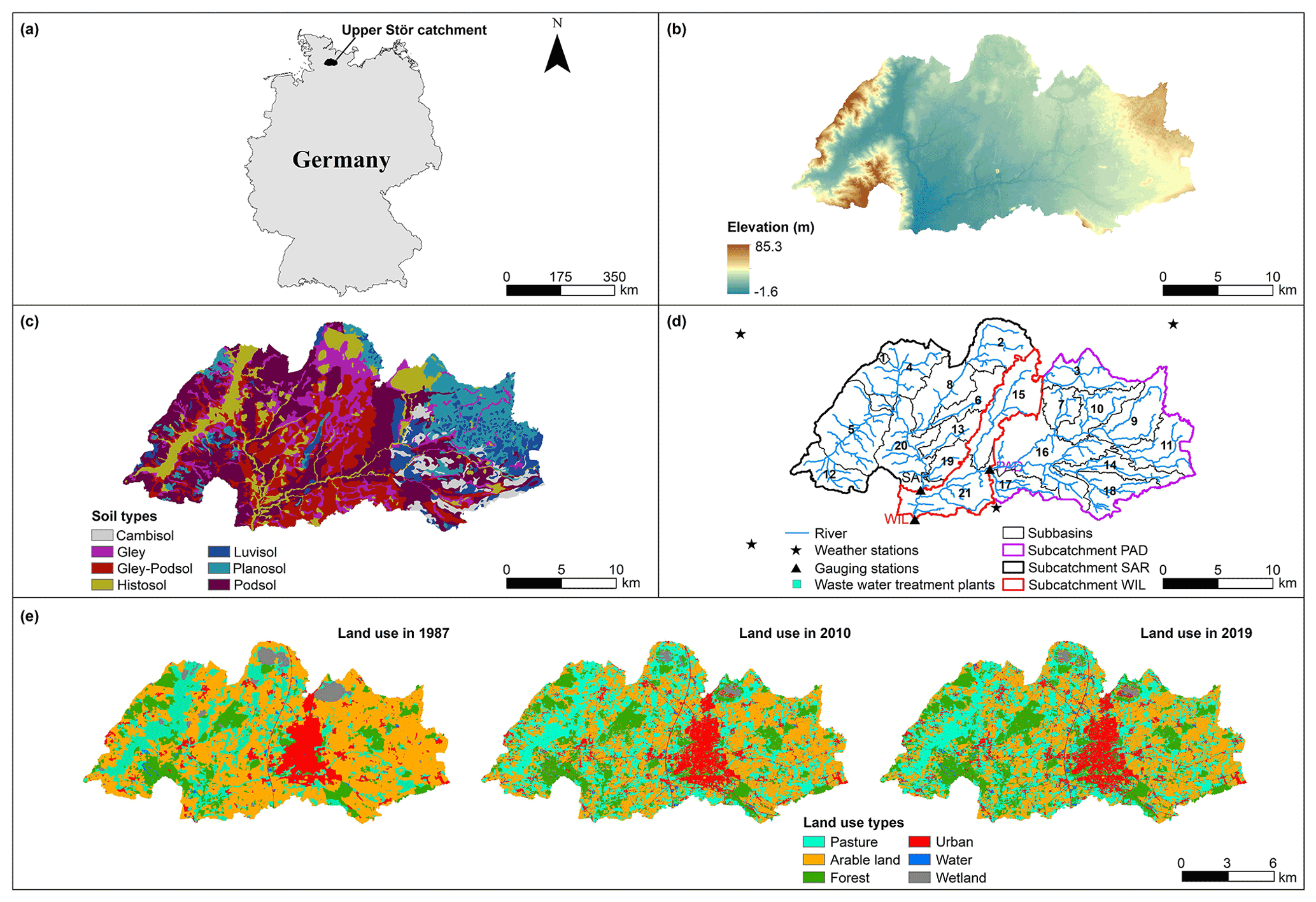
Figure 1 Characteristics of the study area. location of the Upper Stör catchment (a), spatial distributions of the topography (b) (Lverma, 2008) and soil types (c) (Finnern, 1997) of subbasins, weather, and gauging stations, and waste water treatment plants (WWTPs) (d) (Pott, 2014), as well as land use maps (e) (Ripl et al., 1996; Rathjens et al., 2014; Lei et al., 2021).

2.2 Land use data and landscape metrics

Land use maps for 1987, 2010, and 2019 were used to characterize the changes in land use and landscape patterns. The earlier two maps (1987 and 2010) were adapted from Ripl et al. (1996) and Rathjens et al. (2014), respectively, and were based on Landsat 5 (TM – Thematic Mapper) image data at 30 m resolution. The land use map for 2019 was derived from 10 m resolution Sentinel-2 satellite images (Lei et al., 2021). The land use classes were categorized uniformly as (1) arable land (winter cereals, corn, and winter rape and other crops), (2) pasture (meadow, field grass, and rangeland), (3) forest (deciduous and coniferous forest), (4) urban (residential, commercial, and industrial areas), (5) water (rivers, ponds, and lakes), and (6) wetlands (Fig. 1). Water and wetlands are not considered for further analysis, as they comprise only minor and mostly constant percentages.

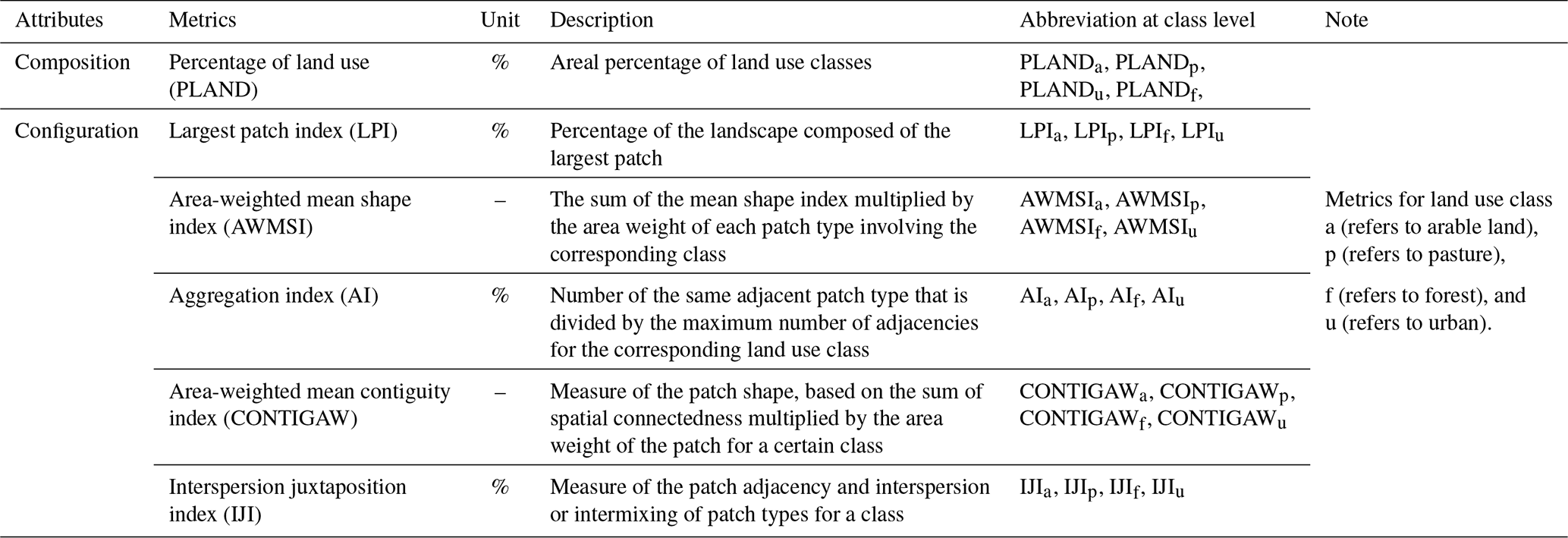
The area percentage of land use class (PLAND) is used as a measure of land use composition. Configuration metrics include the largest patch index (LPI), area-weighted mean shape index (AWMSI), area-weighted mean contiguity index (CONTIGAW), aggregation index (AI), and interspersion juxtaposition index (IJI), considering the dominance, shape, and interconnection of the landscape (Ding et al., 2016; Gémesi et al., 2011). Composition and configuration indices of pasture, arable land, forest, and urban were selected for subsequent analysis (Table 1). They were derived with the help of the software Fragstats 4.2. All indices and their changes were analyzed at the subbasin scale.

Table 1 Description of the landscape metrics selected for the study.

2.3 Hydrological and water quality modeling

2.3.1 SWAT model

The Soil and Water Assessment Tool (SWAT) is a process-based and semi-distributed hydrological model with a continuous time step (Arnold et al., 1998). It is suitable for the simulation of streamflow, sediment, nutrients, and groundwater dynamics in catchments of different sizes (Aghsaei et al., 2020; Tigabu et al., 2020; Bieger et al., 2014; Haas et al., 2016). The computation of water routing, nutrient cycles, and soil erosion is based on hydrologic response units (HRUs) characterized by the same land use, soil type, and slope in the same subbasin representing the spatial heterogeneity of the catchment (Arnold et al., 2013). The HRU-based calculations for the subbasins are routed through the rivers that connect the subbasins (Neitsch et al., 2011).

To accurately represent the groundwater dynamics in this lowland catchment, we applied SWAT_3S, an enhanced SWAT model based on SWAT 2012 revision 582 (Pfannerstill et al., 2014). In comparison to the standard SWAT model application that uses two aquifers, SWAT_3S employs three aquifers by subdividing the original shallow aquifer from SWAT into a fast and a slow aquifer. SWAT_3S was developed in the German lowland catchment of the Kielstau to better represent low flow periods of streamflow and groundwater storage and flow dynamics when compared to the original SWAT version (Pfannerstill et al., 2014). It was also successfully applied to the lowland catchment of the Treene, proving its usefulness for modeling nutrients as well (Haas et al., 2016, 2017).

Table 2 Overview of SWAT model calibration and validation.

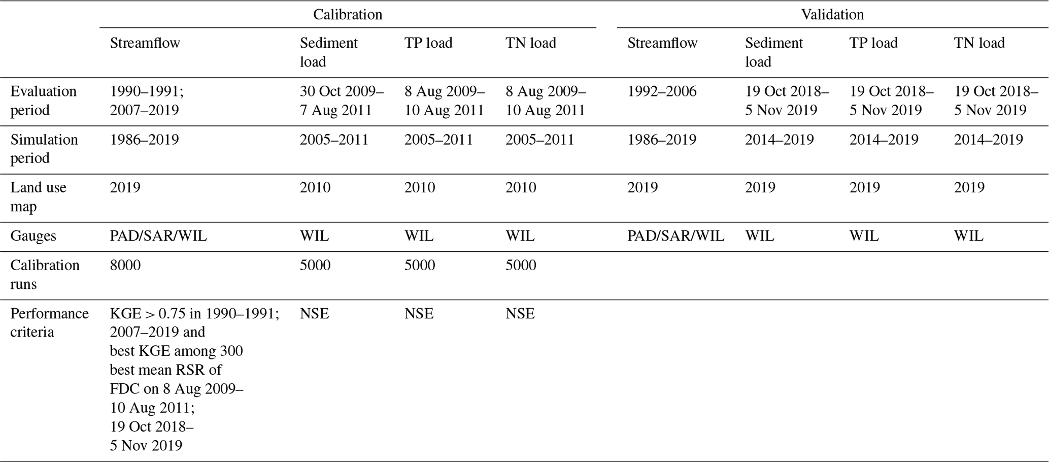
PAD – Padenstedt; SAR – Sarlhusen; WIL – Willensharen; NSE – Nash–Sutcliffe efficiency; KGE – Kling–Gupta efficiency; RSR – ratio of root mean square error to the standard deviation of the observations; FDC – flow duration curve.

2.3.2 Model databases and setup

SWAT requires topography, soil, land use, and hydrometeorological input data. Topography data were obtained from a digital elevation model (DEM) in 5 m resolution (Lverma, 2008) and used to delineate the watershed into 21 subbasins. Soil data and attributes for SWAT were derived by Pott and Fohrer (2017b) from a soil type map (Finnern, 1997). The land use map for 2019 was used to build the model. The 3-year crop rotations (winter wheat/winter wheat/corn; winter rape/winter wheat/corn; corn/corn/corn) were adapted from Oppelt et al. (2012) and implemented for the respective land use classes. Agriculture management schedules and fertilization (e.g., application rates of N, P fertilizers, and manure at different crop growth stages) were determined according to the actual guidelines of agriculture practices (LWK, 1991 and 2011; KTBL, 1995 and 2008; Kühling, 2011). From the DEM, four slope classes (<1 %, 1 %–2 %, 2 %–5 %, and >5 %) were defined. Slope, soil, and land use classes were combined to obtain 3618 HRUs in the catchment. The HRUs were generated without excluding any HRUs by thresholds for land use, soil, or slope class percentages to allow for a better spatial representation. To accurately represent lowland hydrology, drainage tiles were considered based on the estimated distribution of drained areas in the catchment (Venohr, 2000). We adapted drainage parameter values for DEP_IMP (1200 mm), DDRAIN (875 mm), TDRAIN (24 h), and GDRAIN (61 h) from a previous modeling study in the catchment (Pott and Fohrer, 2017b). Waste water treatment plants (WWTPs) were implemented as point sources, using data from monthly measurement campaigns in 2009 and 2010, and WWTP data vary with space and seasons (Pott, 2014). Daily values of temperature (max and min), solar radiation, humidity, and wind speed are available from 1990 to 2019 for the climate station of Padenstedt (DWD, 2020a). Precipitation data are available for four stations (DWD, 2020a; Fig. 1). Daily streamflow was measured at the gauges in Padenstedt (PAD), Sarlhusen (SAR), and Willenscharen (WIL) from 1990 to 2019 (LKN, 2020a). Daily sediment and nutrient data were both obtained during two measurement campaigns, i.e., August 2009–August 2011 and October 2018–November 2019 in Willenscharen. Daily mixed samples were taken by an automatic and cooled sampler from a depth of 0.30 m above the river bed at the central section of the stream. They were analyzed according to German standard procedure for water analysis (Deutsches Einheitsverfahren, 1997) in the laboratory of the Department of Hydrology and Water Resources Management at Kiel University. Total suspended sediment concentration was measured by filtering 1 L of the water sample through 0.45 µm cellulose acetate filter paper and drying at 105 ^∘C. The concentration of total phosphorus (TP) was determined by spectrophotometry, according to DEV H36 and DEV D11, while total nitrogen (TN) was measured by chemiluminescence detection according to DEV H3. Each measurement of TP or TN concentration from unfiltered samples was performed based on a blank comparison analysis of distilled water and triplicate analysis of subsamples. Their concentrations were determined by the arithmetic mean values of any two subsamples with the smallest measurement differences (less than <10 %). Based on the measurements of daily concentration and streamflow, the respective daily load of sediment, TP, and TN were calculated.

2.3.3 Model calibration and validation

The variables of daily streamflow (1), sediment (2), TP (3), and TN (4) were calibrated separately and stepwise. The number in the parentheses denotes their respective calibration order, i.e., streamflow was calibrated first, followed by sediment, TP, and TN. An overview of the calibration and validation details for each variable is provided in Table 2.

Preliminary parameter ranges were selected based on experiences with the SWAT model in the Stör catchment (Pott and Fohrer, 2017b) and other German lowland catchments (i.e., Kielstau and Treene catchments; Haas et al., 2016; Lam et al., 2012; Pfannerstill et al., 2014), as well as in relevant studies from other countries (Aghsaei et al., 2020; Boongaling et al., 2018). The final ranges of calibration parameters (Table S1 in the Supplement) were determined based on the sensitivity of the parameters to model outputs as derived from 2000 trial runs following the method used by Guse et al. (2020), in which model simulations are iteratively repeated with successively constrained parameter ranges.

Parameter sets were generated from the derived parameter ranges using Latin Hypercube Sampling in the R package FME (Soetaert and Petzoldt, 2010). For each of these 8000 (streamflow) and 5000 (sediment, TP, and TN loads) independent parameter sets, model runs were conducted, with each involving a warm-up period (4 years), and evaluated using multiple performance criteria to select the best parameter set. To this end, the objective functions of the Nash–Sutcliffe efficiency (NSE), Kling–Gupta efficiency (KGE), and percent bias (PBIAS), which were proposed in Guse et al. (2014) and Moriasi et al. (2007), were applied. For an accurate representation of all segments of the hydrograph (very high, high, middle, low, and very low periods), the additional signature measure of RSR (ratio of root mean square error to the standard deviation of the observations) was used (Haas et al., 2016; Zambrano-Bigiarini, 2020). The definition of each objective function is provided in Sect. S1 in the Supplement.

First, streamflow was calibrated at three gauges. The two upstream gauges of Padenstedt (PAD) and Sarlhusen (SAR) were used to select the best parameter sets for the respective subcatchments first (Fig. 1). Then, the best parameter set for the area downstream of PAD and SAR and upstream of the outlet gauge Willenscharen (WIL) was selected. For each of the three streamflow gauges, we preselected the parameter sets that yielded a KGE > 0.75 for the streamflow calibration period. To accurately represent the streamflow dynamics during the periods of water quality measurements (August 2009–August 2011 and October 2018–November 2019), the mean RSR for the five flow duration curve (FDC) segments during these periods was assessed, and the best 300 streamflow parameter sets indicated by a low RSR were selected. From these 300 sets, the final parameter set yielding the highest KGE in these periods was selected. Calibration and validation periods (Table 2) were defined based on an equal representation of dry, normal, and wet years, according to the annual precipitation.

Second, with the derived set of best hydrological parameters, model runs for 5000 different sediment calibration parameter sets were carried out, and the best model run was selected based on the highest NSE. Third, this model was run for 5000 different sets of TP calibration parameters, and the best model run was similarly selected using the NSE. Finally, based on the so-far derived best parameters, another 5000 model runs for TN calibration were carried out, and the best model run indicated by the highest NSE was selected. To accurately represent peak loads and their dynamics, the NSE was selected as a single criterion for the water quality variables. Evaluation and processing of the model data were carried out in R, using the packages hydroGOF (Zambrano-Bigiarini, 2020) and zoo (Zeileis and Grothendieck, 2005).

2.3.4 Model application

Applying the best respective parameter sets, the model was run for three land use scenarios. Each scenario simulation was run from 1990 to 2019, using one of the three land use maps (in 1987, 2010, and 2019). As agriculture in 1987 was generally classified, it was split into corn (12 %), rapeseed (29 %), and wheat (59 %) randomly distributed in the catchment in SWAT model, according to the statistical data from the Statistical Office Schleswig-Holstein (1992–2013). For the three scenario simulations, all other inputs i.e., DEM, soil data, weather data, waste water quality data, management practices, and fertilization were kept constant, and the calibrated parameters were adapted. The respective differences in the mean annual value of each response variable (i.e., actual evapotranspiration – ET; surface runoff – SQ; base flow – BF; water yield – WYLD; sediment – SED; TP or TN load) were obtained by comparing the results from two scenario model runs (see Sects. S2 and S3). They can be referred to as the respective changes driven by land use changes during the corresponding periods of 1987–2010, 2010–2019, and 1987–2019. The modeled results were used to explore the influences of land use changes (LUCCs) on the changes in the response variables. Furthermore, the contributions of LUCCs on changes in ET, SQ, BF, and WYLD, as well as in SED, TP, and TN, at the subbasin scale were evaluated, and key impacts from LUCCs were identified.

2.4 Partial least squares regression

Combining the features of principal component and multiple linear regression analyses, partial least squares regression (PLSR) is a robust multivariate analysis method for determining the relationship between two sets of variables. It is powerful enough to deal with multi-collinear predictor variables. The principle of PLSR is to extract a few latent components from original predictor variables that carry as much variation as possible and which are, meanwhile, most likely to predict the variation in the response variable. Detailed information on the underlying theory and algorithms of PLSR is available in Abdi (2010).

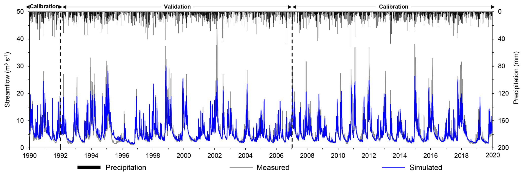
Figure 2 Comparison of measured and modeled daily streamflow during the calibration and validation periods in Willenscharen.

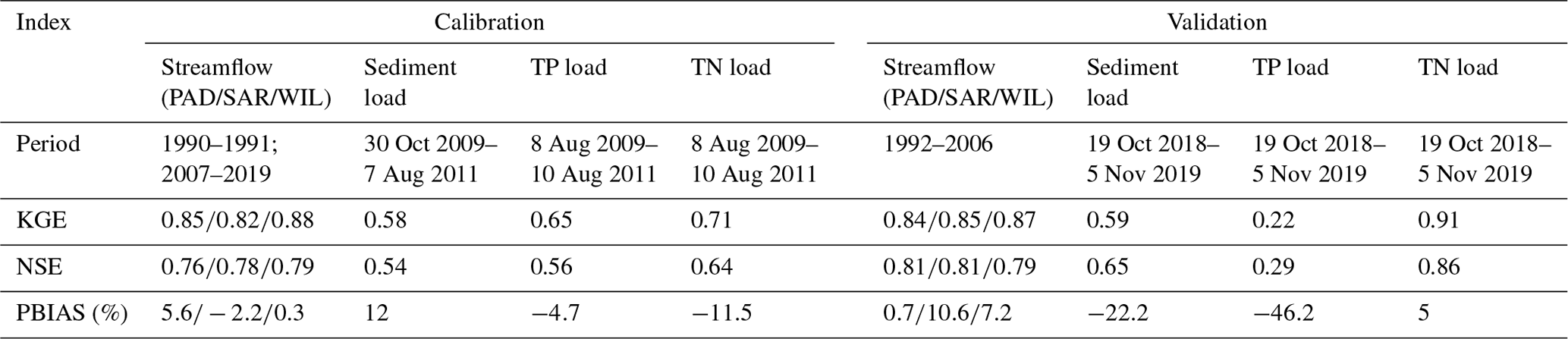
Table 3 Performance metrics for the model calibration and validation periods.

In this study, PLSR was used to reveal the contribution of changes in land use classes on the variation in ET, SQ, BF, WYLD, SED, TP, and TN across three time steps (1987, 2010, and 2019). The predictor variables were the absolute changes in area percent (PLAND) and landscape metrics (LPI, AWMSI, AI, CONTIGAW, and IJI) of four main land use classes (arable land, pasture, forest, and urban). The response variables included the absolute changes in the mean annual values of ET, SQ, BF, WYLD, SED, TP, and TN loads at the subbasin scale modeled under different land use conditions in 1987, 2010, and 2019. PLSR models for all of these response variables were constructed. The absolute change in each land use indicator was calculated using Eqs. (5)–(7), while that in each response variable was calculated using Eqs. (8)–(10), as shown in Sect. S3. A cross-validation was performed with 50 random repetitions on 10 equal segments of the data set. It was used to determine the number of optimal components of the PLSR model to obtain a desirable balance between the explained variation in the response (R²) and predictive power of the model (measured as cross-validated goodness of the prediction, Q²). The cumulative predictive ability (cumulative goodness of prediction, Q² cumul.) and the cross-validated root mean squared error (RMSECV), as the difference between actual and predicted values, were determined for each model (Yan et al., 2013). The regression coefficients (RCs) signify the direction and extent of the effect of LUCC predictor variables. The variable importance for the projection (VIP) quantifies the importance of the predictors. According to Wold's assessment criterion, a predictor with VIP < 0.8 is assessed as being less important (Boongaling et al., 2018; Wold et al., 2001). To achieve model parsimony, the following PLSR modeling procedures were conducted: First, an initial simulation of PLSR is run using all predictors. Next, new PLSR models are run by iteratively excluding the predictor with small variable importance (VIP) until the modeling procedure resulted in acceptable variable importance or only two predictors remained. The number of components of candidate PLSR model was determined so that the Q² cumul. is maximized (Shi et al., 2013).

All the PLSR analyses were performed with the R packages of pls (Mevik et al., 2020) and mdatools (Kucheryavskiy, 2020).

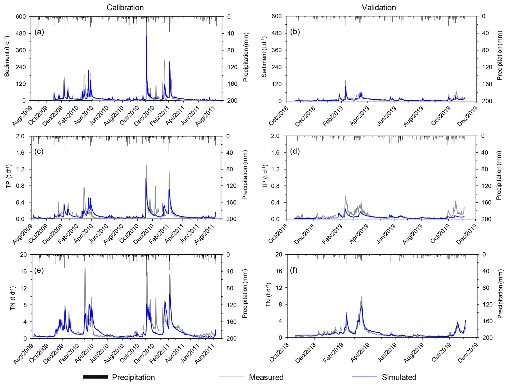
Figure 3 Comparisons between measured and modeled daily loads of sediment, total phosphorus (TP), and total nitrogen (TN), respectively, for calibration (a, c, e) and validation (b, d, f) periods.

3 Results and discussion

3.1 Model performances for calibration and validation periods

As shown in Table 3, for streamflow, the model obtains NSE and KGE values above 0.75 and absolute PBIAS values below or slightly above 10 %. These values indicate a good to very good model performance for depicting daily streamflow in the catchment according to the criteria for model evaluation (Moriasi et al., 2007). For the daily TN load, the model shows a satisfactory to very good performance, as indicated by an NSE between 0.64 and 0.86 and absolute PBIAS values below 15 %. For the sediment load, the model achieves a satisfactory to good performance, as indicated by NSE (0.54–0.65) and PBIAS (−22.2 % to 12 %) values. The model simulates TP load with an unsatisfactory (validation) to satisfactory (calibration) performance, which is assessed by NSE below and above 0.5, respectively. The worse TP model performance may be due to the short and possibly different conditions during calibration and validation periods. Nevertheless, PBIAS for TP model is still within the acceptable performance range ($\pm \mathrm{40}\le \mathrm{PBIAS}<\pm \mathrm{70}$; Moriasi et al., 2007). It should be noted that the performance ranges from Moriasi et al. (2007) refer to a monthly time step, whereas we used a finer temporal scale (daily step), on which it is usually harder to achieve a good model representation (Tan et al., 2021; Pfannerstill et al., 2014; Pott and Fohrer, 2017a). We, therefore, conclude that, even for daily TP, the model performance is acceptable, particularly with regard to the study purpose of analyzing long-term changes in the water and matter balance.

Overall, modeled and measured daily values show clear consistency in their dynamics (Figs. 2 and 3). Differences mainly appear for low flow periods in summer and particularly for a few peak flows in winter. Specifically, a few flood peaks are underestimated in winter, e.g. on 27–28 February 2002, 5–6 January 2012, and 24–25 December 2014. This might be related to an insufficient representation of snow and the deficiencies in single-event flood routing in the model (Lam et al., 2012). The underestimation of peak streamflow in winter was also observed in other rural lowland catchments of Treene (Haas et al., 2016) and Kielstau (Lam et al., 2010) in northern Germany. Sediment loads are overestimated during the calibration period and slightly underestimated during the validation period, mainly for a few peak values. The incorrect estimation might be due to the fact that the river sediment load is also influenced by tile drains and bank erosion in lowland catchments (Kiesel et al., 2009), while SWAT primarily takes into account sheet erosion. Nevertheless, some peaks, e.g., in November and December 2009 and March 2019, are very well depicted. A similar behavior is observed for modeling the TP load, with a slight overestimation of TP in summer (April–June in 2009 and 2019) and an underestimation of a few peaks in winter (November–March). TN is generally well represented, except for only a few underestimations of extreme peaks in winter (e.g., early March or November 2010). Overall, the underestimation of some peak loads of sediment, TP, and TN might be attributed to the underestimation of corresponding peak flows.

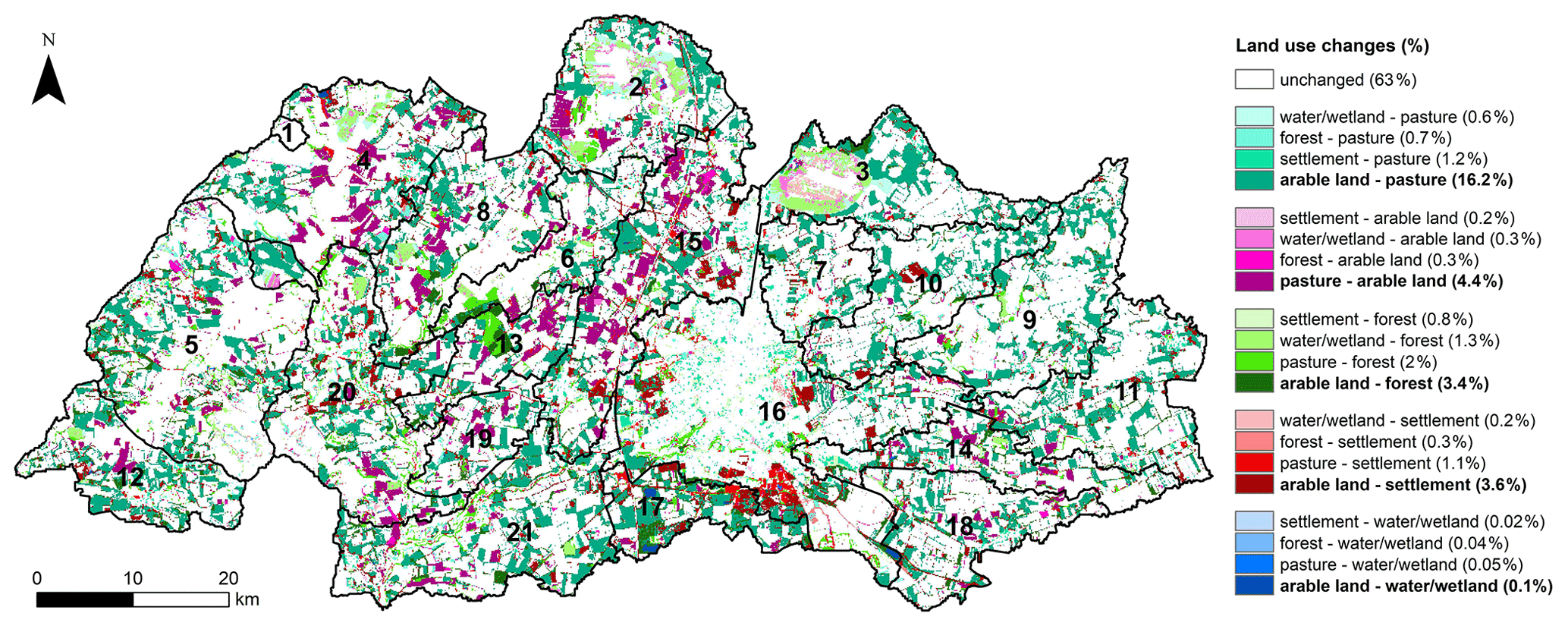
Figure 4 Spatial distribution of land use changes between 1987 and 2019 in the Stör catchment. Individual land use change types are marked by different colors. The percentage of each change type, calculated as percentage of the catchment area, is given in the parentheses. The strongest change is marked in bold.

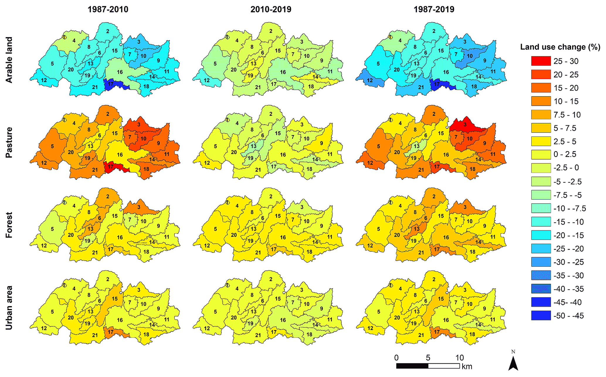
Figure 5 Spatial distribution patterns of the changes in each land use type between the years 1987, 2010, and 2019.

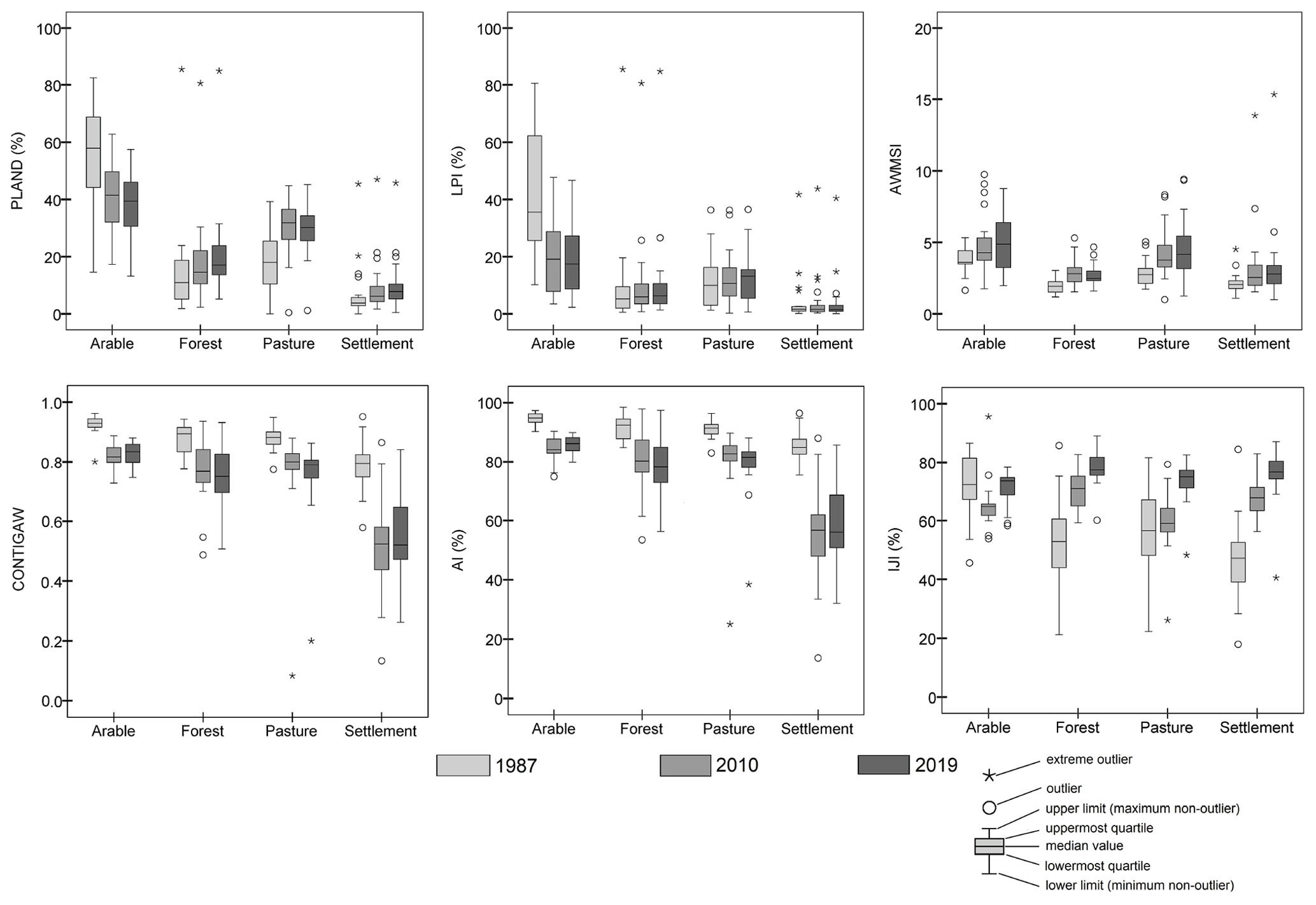
Figure 6 Changes in land use metrics between the years 1987, 2010, and 2019 in the Stör catchment.

3.2 Characteristics of land use change

Land use changes between 1987 and 2019 vary across the catchment (Fig. 4). This is indicated by the individual dynamics in the four main land use classes of arable land, pasture, forest, and settlement area. Arable land has been decreasing and has primarily been replaced by pasture (by 16.2 % of the catchment; dark cyan in Fig. 4). The decrease in arable land in the northeast (e.g., subbasins 3 and 9–11) is more pronounced than in the northwest (e.g., subbasins 2, 4, 6, and 8), where pasture was sometimes converted to arable land (dark pink; Fig. 4). Conversely, pasture shows an increasing trend over the period of observation. The increase in the east is stronger compared to the west of the catchment (Figs. 4 and 5). The change in pasture is, in part, associated with the stream restoration, including stabilizing the river shore and increasing riparian vegetation (Dickhaut, 2005; Gessner et al., 2010). Besides, agricultural grasses may have been included in the pasture class due to the classification approach. Forest areas also show an increasing trend, as indicated by green colors in Fig. 4, with a strong increase in the lowlands of the middle (subbasins 6 and 13) and southern parts (subbasin 17; Fig. 5). The urban area has expanded mainly around the city of Neumünster (subbasin 15 and 17; Fig. 5).

In addition, the subbasin-scale land use metrics varied substantially between 1987, 2010, and 2019 (Fig. 6). The mean area percent (PLAND) per subbasin declined for arable land (PLAND_a) by 16 % and 3 % during the periods of 1987–2010 and 2010–2019, respectively. In contrast, subbasin-averaged pasture (PLAND_p) increased for the period of 1987–2010 by 12 % but decreased slightly from 2010 to 2019 by 0.8 %. Both forest (PLAND_f) and urban (PLAND_u) areas have steadily increased from 1987 and over 2010 to 2019. Similar trends are found in the metrics of the percentage of largest patch index (LPI) and the interspersion juxtaposition index (IJI). The subbasin average of LPI for arable land has decreased by 20 % from 1987 to 2019, whereas the LPI of other land use classes shows a slight and stable increase. The IJI of arable land displays an overall slight increase from 1987 to 2019, while the IJI values of other land uses have steadily and notably increased (with a net increase up to over 20 %). Both the area-weighted mean contiguity (CONTIGAW) and aggregation (AI) of each land use class have decreased over time, whereas the area-weighted mean shape index (AWMSI) has increased continuously and slightly. Despite similar changing directions of the land use patterns in the periods of 1987–2010 and 2010–2019, land use has been subject to more alterations in the former period than in the latter. Additionally, CONTIGAW, AI, and IJI of arable land exhibit opposite trends in the two periods, with a decrease from 1987 to 2010 and a slight increase from 2010 to 2019.

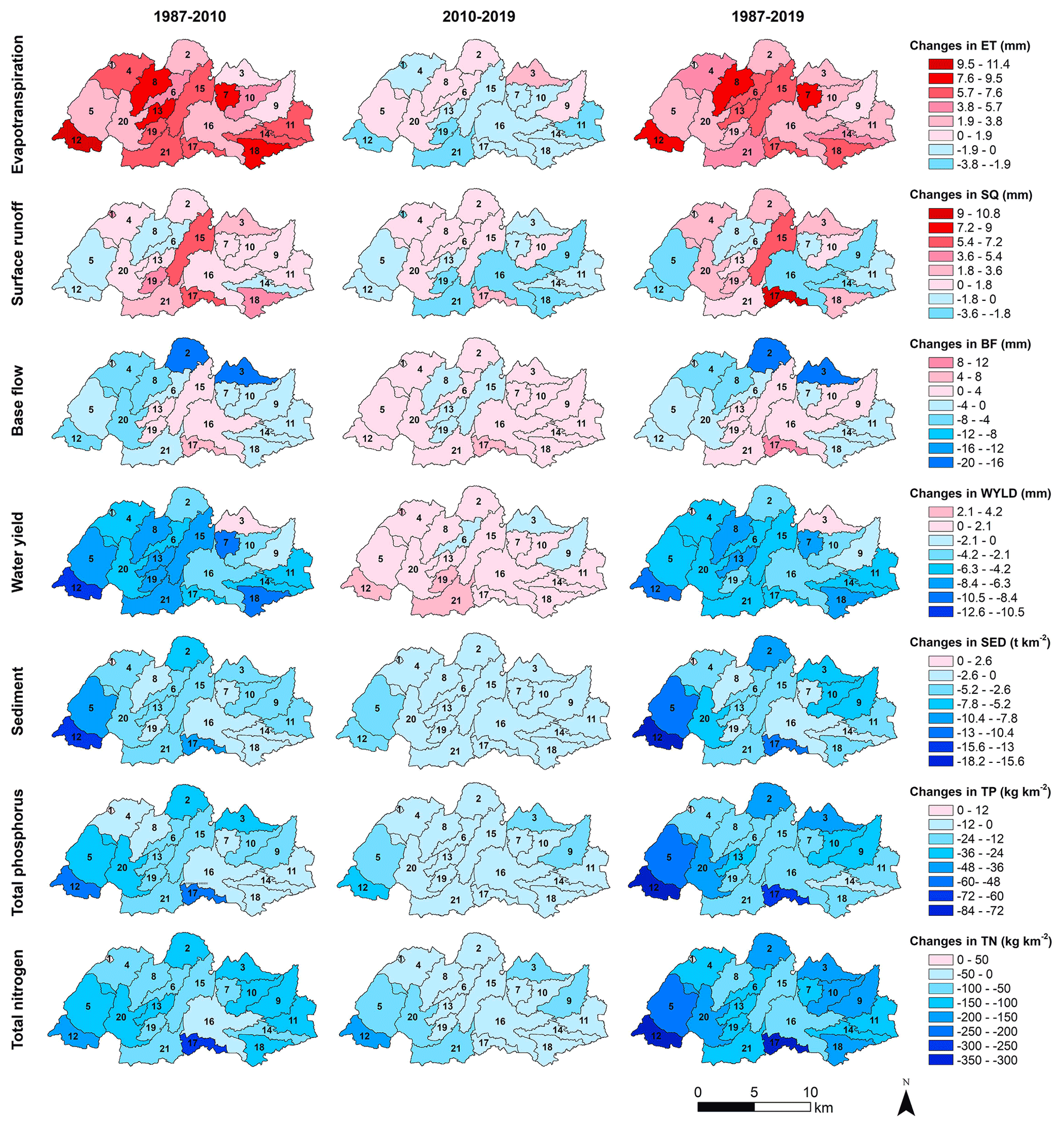
Figure 7 Spatial distribution of changes in water quantity and water quality variables during the periods of 1987–2010, 2010–2019, and 1987–2019 at the subbasin scale.

3.3 Differences in changes in water quantity and quality

Using the results from the three different scenario model runs based on three land use maps of 1987, 2010, and 2019, we calculated changes in water quantity and quality. The spatial distribution of the variations in the modeled subbasin-scale actual evapotranspiration (ET), surface runoff (SQ), base flow (BF), water yield (WYLD), loads of sediment (SED), total phosphorus (TP), and total nitrogen (TN) between 1987, 2010, and 2019 are shown in Fig. 7. ET and SQ are mostly characterized by increases of up to 10.8 and 11.4 mm, respectively, from 1987 to 2019, with slight decreases by up to 3.8 mm in several subbasins between 2010 and 2019. The most significant increase in ET occurs in subbasins which show a larger increase in forest from 1987 to 2019, such as subbasins 8, 12, and 17 (Fig. 5). SQ shows a stronger increase in the middle–western subbasins that experienced a larger expansion of urban areas (Fig. 5), with the strongest increase of SQ occurring in subbasins 15 and 17 that experienced the largest increase in urban area between 1987 and 2019. This might be attributed to the increased impervious surface which facilitates the generation of surface runoff and reduces confluence time (Anand et al., 2018; Sood et al., 2021). Contrarily, BF and WYLD have decreased by up to 20 and 13 mm, respectively, in most subbasins in the periods 1987–2010 and 1987–2019. However, a few subbasins in the central part of the catchment exhibit a slight increase in base flow, which is probably attributed to a greater contribution of shallow groundwater in the central lowland areas to low flow periods than in the steeper eastern and western steeper areas. The loads of SED, TP, and TN show notable decreasing trends from 1987 to 2019. Pronounced reductions in SED (7.8–18.2 t km⁻²) occur in the relatively steeper northeastern corner (e.g., subbasins 3 and 9–10) and the southwestern corner (e.g., subbasins 5 and 12) and subbasin 17, while the decrease is weaker in the midwest. Overall, the changes in TP and TN loads show a weak decrease in the (mid-) west, and more pronounced decreases are in the east and steeper areas in the southwest of the catchment (Fig. 7). The spatial differences may be related to the more intense exchange between groundwater and surface water and a higher contribution of nutrients from groundwater to the stream in the lowland. The most pronounced net decrease in TP and TN loads are observed in subbasins 12 and 17, corresponding to the largest decrease of arable land percentage (50 % in subbasin 17; 30 % in subbasin 12) between 1987 and 2019. The single subbasin that has experienced a slight increase in sediment or TP load is subbasin 1, which is characterized by the lowest reduction in arable land and a minor decrease in forest. The most significant decrease in nutrients and sediment has occurred in subbasins which have experienced notable increases in pasture or forest and a decrease in arable land, e.g., subbasins 12 and 17 (Fig. 5). Overall, variations in surface runoff, sediment, TP, and TN are depicted by spatially explicit patterns on the subbasin scale. It is necessary to consider this spatial heterogeneity, when establishing management measures, in order to improve water quality.

3.4 Influences of changes in land use metrics on water quantity and quality

3.4.1 Contributions of LUCC to changes in water quantity and quality

A summary of the PLSR models separately constructed for ET, SQ, BF, WYLD, SED, TP, and TN is provided in Table 4. The prediction plots for the seven variables, by applying the PLSR models, are shown in Fig. 8. The changes in water quantity and quality could be reasonably explained by the constructed PLSR models ($\mathrm{0.61}<R^{\mathrm{2}}<\mathrm{0.88}$ and $\mathrm{0.57}<Q^{\mathrm{2}}<\mathrm{0.85}$; Table 4). The comparison of the actual and predicted values (in Fig. 8) illustrates the accuracy of the model calibration and cross-validation. For the ET and WYLD models, the percentage of the unexplained variation decreases with increasing number of components, whereas the prediction error of cross-validated observations (indicated by cross-validated root mean squared error – RMSECV) is minimal, with one or two components, respectively. This indicates that adding more components does not improve the correlation with the residuals of the response variables (Onderka et al., 2012). Overall, 60.5 % and 68.3 % of the variations in the changes in ET and WYLD can be explained by the first component and the first two components, respectively. Adding other components does not strongly increase the cumulative explained variations (only by +4.2 % to 5.4 %) in ET, and WYLD changes from 1987 to 2019 (Table 4). For SQ, two components are extracted for the PLSR model, with 58.9 % of variation being explained with the first component, and cumulative explained variations increase to 81.3 % when adding the second component. For all other variables, the minimum RMSECV is achieved with models using five components. For base flow, 37.4 % of the variation in the dynamics is explained by the first component, cumulatively 64.2 %, adding the second component, and ultimately 87.7 %, with a consecutive addition of the third, fourth, and fifth component. For the changes in loads of sediment, TP, and TN, the first component of the models always explains the majority of the variation (43.7 %–63 %; Table 4). With all water quality variables together, approximately 75 % of the changes is accurately explained, on average.

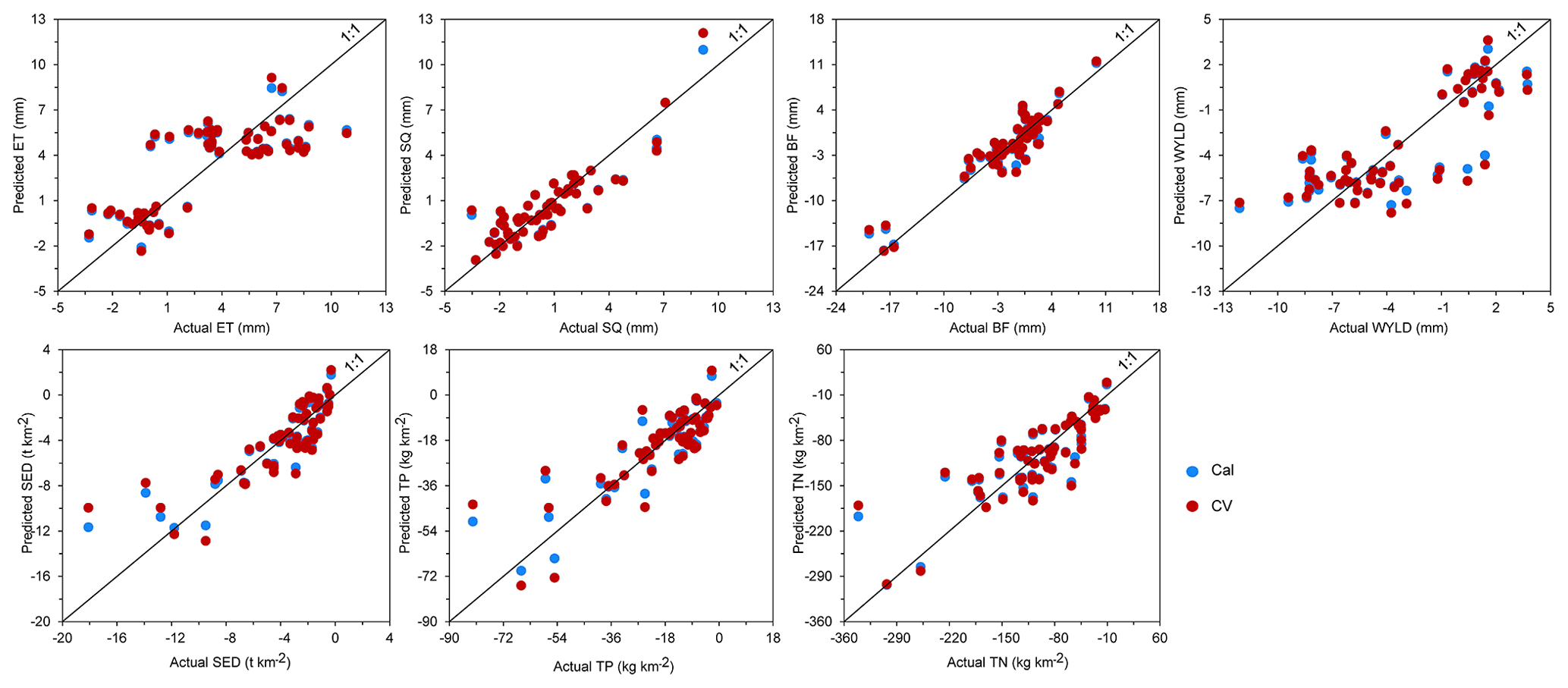
Figure 8 Comparison of subbasin-scale changes in evapotranspiration (ET), surface runoff (SQ), base flow (BF), water yield (WYLD), sediment (SED), total phosphorus (TP), and total nitrogen (TN), as derived from the SWAT model and the predicted values from the PLSR models. The changes were obtained based on land use changes between 1987 and 2010, 2010 and 2019, and between 1987 and 2019, respectively. Cal indicates calibration. CV indicates cross-validation.

Table 4 Summary of the PLSR models of evapotranspiration (ET), surface runoff (SQ), base flow (BF), water yield (WYLD), sediment yield (SED), total phosphorus load (TP), and total nitrogen load (TN) at the subbasin scale.

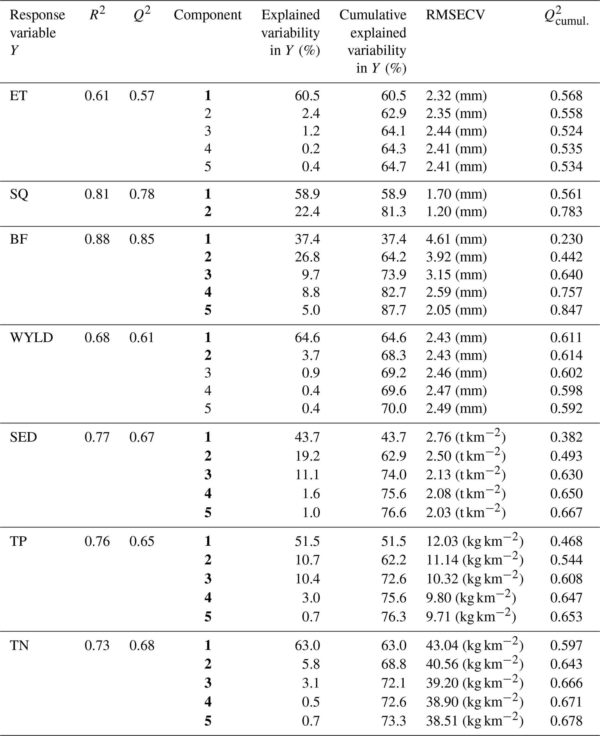
Note: R² indicates the goodness of fit of the model, Q² indicates the cross-validated goodness of prediction, RMSECV indicates cross-validated root mean squared error, and $Q_{\mathrm{cumul}.}^{\mathrm{2}}$ indicates the cumulative cross-validated goodness of predication over all the selected PLSR components. The components selected for each model are highlighted in bold.

Approximately 70 %–80 % of the variations in water quantity and quality dynamics were explained by LUCC, underlining the importance of LUCC for catchment water resources. Better explanations (over 81 %) of SQ and BF by LUCC confirmed the significant influences of landscape heterogeneity on surface runoff and groundwater dynamics (Xu et al., 2020; Kändler et al., 2017; Zhang and Schilling, 2006). Only a quarter of the variations in sediment, TP, or TN cannot be interpreted by LUCC, which demonstrates that changes in rural landscape patterns are essentially important in controlling nutrient pollution. The proportion and spatial arrangement of agricultural land play an important role in the generation and transportation of nutrient pollutants, as previously reported in different catchments worldwide. For example, Zhang et al. (2020b) found that agricultural cultivation on steeper hillsides intensified N and P entries in ponds in the hilly Tianmu Lake catchment in eastern China. Gémesi et al. (2011) identified that the cohesion and contagion of cropland were more important than other land use indicators to account for the variability in TN and TP in the relatively plain lake catchment in Iowa in the central USA. The minor unexplained fraction may be attributed to potential changes in waste water treatment, which sometimes remained constant in our modeling approach. A lower explanation of TP may, additionally, be due to the lower SWAT model performance for TP, the susceptibility of P to soil or geomorphology properties (Maranguit et al., 2017; Noe et al., 2013). More than 60 % of the variations in ET and WYLD are explained by LUCC. The unexplained fraction may be attributed to the different contributions from specific crops (included in SWAT) and the lumped agriculture class, as well as the compensating effect of subbasins (Wagner et al., 2013).

3.4.2 Effects of LUCC predictors on water quantity and quality

According to the PLSR results, each category of the landscape indices, including percentage (PLAND), largest patch (LPI), shape (AWMSI), contiguity (CONTIGAW), aggregation (AI), or interspersion (IJI), plays an essential role in influencing as least one water quantity or quality variable (Table 5). The effects on the changes in ET, SQ, BF, WYLD, SED, TP, and TN are measured using weights, regression coefficients (RCs), and VIP values in the PLSR models. VIPs for predictors included into the models are greater than 0.8. For the ET model, the highest VIPs are obtained from the predictors aggregation index for arable land (AI_a) and the contiguity index for arable land (CONTIGAW_a; VIP = 1.25; RCs = −0.122), followed by PLAND_a (VIP = 1.037; RC = −0.101) and AI_u (VIP = 1.0; RC = −0.1). ET tends to decrease with larger aggregation (AI_a) and contiguity (CONTIGAW_a) indices, and arable land percent (PLAND_a; negative RCs), whereas it increases with more pasture (PLAND_p; positive RC). In the case of surface runoff, the first and second components of the model are dominated by PLAND_u on the positive side, with a minor positive effect from PLAND_a on the second component (Table 5). The urban area percent (PLAND_u) obtains the largest VIP of 1.173 and is identified as the most important influencing the change in surface runoff. Surface runoff increases with an increase in arable (PLAND_a) and urban areas (PLAND_u; RCs = 0.403 and 1.161, respectively). For base flow, in addition to arable land, pasture plays a key role in explaining its variation. Arable land (PLAND_a), pasture (PLAND_p) percent, and the area-weighted shape index of pasture (AWMSI_p) obtain the largest VIPs of 1.259, 1.03, and 1.063, respectively. All show negative correlations with base flow. AI_a and CONTIGAM_a are important predictors for water yield, with large VIPs of 1.226 and 1.218, respectively. Their higher values result in an increase in water yield. For sediment, TP or TN models, the selected components are dominated by areal percentages of arable land and pasture, in addition to the landscape metrics of arable land. The models obtain the largest regression coefficients or VIPs for PLAND_a, LPI_a, or PLAND_p. They have VIPs of 1.0113–1.173 for sediment, 1.089–1.305 for TP, and 1.005–1.232 for TN, respectively. Inferred by the RCs, an increase in sediment, TP, or TN occurs with increasing arable land (RCs of 0.602–0.884), while a decrease may occur with higher percentage of arable land in the largest patches (LPI_a; RCs of −0.74 to −0.225) or with more pasture area (RCs of −0.693 to −0.122).

Table 5 Regression coefficients (RCs), VIP, and weight values of each PLSR model.

Note: VIP values greater than 1 were marked in bold. The absolute weights greater than 0.1 were marked in italics.

LPI_a, AI_a, and CONTIGAW_a are the most important landscape structure indicators affecting water quantity or quality (VIP ≥ 1 most of the time; Table 5). AI_a and CONTIGAW_a have positive impacts on WYLD, while there are negative impacts on ET. By definition, AI_a and CONTIGAW_a would increase, respectively, when arable landscape patches are more clumped and contiguous (Shi et al., 2013; Uuemaa et al., 2009). Agriculture in more clumped and connected land patches with fewer edges has been proven to show a higher capability of reducing the infiltration, compared to small scattered patches (Boongaling et al., 2018), which may result in the increase in the water yield. Our results also corroborate with Ayivi and Jha (2018), who reported that increased water yield and base flow occur with increasing cohesive and aggregated agriculture in a moderate-altitude catchment (i.e., Reedy Fork–Buffalo Creek catchment, USA). Negative impacts on ET may be explained by the interactive changes between arable land and pasture, i.e., arable land has been increased at the expense of pasture and vice versa. Likewise, Shawul et al. (2019) observed that reduction in pasture would result in a decrease in ET in an agriculture-dominated and moderate-altitude catchment (the Upper Awash catchment, Ethiopia). The negative effect of AWMSI_p on base flow implies that the coarse grass landscape has a higher capacity of absorbing and intercepting rainfall, thereby resulting in a lower base flow. Though landscape metrics are more often used to explain water quantity than quality variables (Table 5), the negative influences of LPI_a on sediment and nutrients, and positive influences of AWMSI_a on sediment and TP cannot be overlooked. Similar findings were observed in hilly catchments, where scattered and complicated agriculture patches are susceptible to soil erosion and, thus, water quality deterioration (Yan et al., 2013; Nafi'Shehab et al., 2021).

The change in the percentage of arable land is most responsible for water quantity and quality dynamics, with VIP values greater than 1 for all response variables but WYLD. This may be explained by the fact that the decrease in arable land is the strongest. The negative correlations between PLAND_a and evapotranspiration (ET) and base flow (BF) imply that conversion of arable land to, e.g., pasture or forest would result in increased ET and BF, due to the higher capability of plant evapotranspiration and slower water transmission, which is in agreement with previous findings that perennial vegetation is more likely to increase ET (Peel et al., 2010; Li et al., 2017), and the decrease in agriculture leads to increased annual base flow (Basuki et al., 2019). Less interception by crops and additional surface runoff resulting from the implementation of tillage practices (e.g., tractor roads) can result in increased surface runoff (SQ). The lower ET amount of crops compared to pasture and forest is in part responsible for the increase in WYLD. Soil erosion might be accelerated due to uncovered and fragile soil by tillage practices implemented in cultivated areas and the increased surface runoff. N and P pollution is prone to occurring in arable areas, which have a high risk of generating nutrient pollutants from excessive fertilizer or manure and eroded soil particles. The positive relationships between arable land percent and SQ, WYLD, SED, TP, and TN loads are found in other studies around the world as well (Sood et al., 2021; Wang et al., 2019; Wagner et al., 2013; Mirghaed et al., 2018; Zhang et al., 2020a). Pasture shows a positive influence on ET and negative influences on sediment, TP, and TN. This also illustrates that more grassland (or rangeland) would increase the plant evapotranspiration process. Pasture can improve water quality due to reduced soil erosion and nutrient transportation rate and the high uptake and infiltration of nutrients by vegetation cover. Relevant studies (Li et al., 2008; Hatano et al., 2005; Ding et al., 2016; Zhang et al., 2020a) have often observed that semi-natural vegetation (e.g., forest, bushland, or grassland) is beneficial for good water quality in river- or lake-dominated catchments, due to the higher capability of filtering contaminants and reducing their inputs and decreasing surface runoff.

By applying the quantitative results that the increases in arable or pasture areas most significantly intensify or reduce the risk of soil erosion and nutrient pollution, respectively, individual subbasins can be identified as nutrient pollution sources or sinks. Based on these results, it is possible to develop a set of more targeted strategies to effectively control diffuse pollution at a spatial scale. At the same time, the best management practices, such as proper fertilization, abatement of traditional tillage, crop rotation, and vegetation buffers, are important for improving water quality in rural catchments (Haas et al., 2017; Pott and Fohrer, 2017a). Urban expansion is most important in influencing surface runoff, as the increase in urban area percent results in an increase of it (regression coefficient value > 1.16; Table 5). Similar results have been found, e.g., by Shi et al. (2007), who discovered that increased urbanized land led to increased surface runoff, by increasing flood peaks and decreasing surface runoff confluence time, in a typical urbanized region (Shenzhen) in China. Unlike previous findings (Yan et al., 2013; Wang et al., 2018), forest properties have not exerted significant influences, probably due to only minor temporal changes in some landscape metrics, e.g., area percent (PLAND), dominance (LPI), and shape (AWMSI) of forest (Fig. 6).

4 Conclusion

In this study, the separate contributions of changes in land use on the dynamics of seven water quantity and quality variables, i.e., actual evapotranspiration (ET), surface runoff (SQ), base flow (BF), water yield (WYLD), sediment (SED), total phosphorus (TP), and total nitrogen (TN) loads were quantified by applying an integrated approach of hydrological modeling (SWAT) and partial least squares regression (PLSR). The influences of the changes in individual land use indicators on changes in water quantity and quality were measured and identified using a scenario analysis for three different land use maps of the past.

The modeling analysis of the effects of past land use changes showed that water quality and quantity variables varied in different ways on the subbasin scale. SED, TP, and TN decreased more strongly in the eastern and western parts than in the middle lowlands, implying that a higher contribution of nutrients by groundwater can mediate the influences of land use change. Based on a PLSR analysis, about 75 % of the modeled variations in water quality and quantity variables can be accurately explained by land use indicators. The change in arable land is inferred to be most important for water quality and quantity dynamics, as arable land indicators mostly showed a greater importance (measured by VIP > 1) for more response variables compared to other indicators. Looking at the most significant impacts, the expansion of arable land (PLAND_a) caused BF to decrease, and urbanization expansion resulted in increased SQ. More aggregated and connected arable land patches led to a decrease in ET and an increase in WYLD. Arable land expansion exacerbated soil erosion and P and N pollution, whereas an increase in pasture helped to relieve nutrient pollution problems. These results underline that water quality and quantity variables are affected by land use changes in different ways. To achieve good water quality, the dynamics in the extent and the spatial configuration of arable land require special attention. The spatial assessment of changes in water quantity and quality variables in this study provides a basis for an informed and location-specific management of land and water resources.