the Creative Commons Attribution 4.0 License.
the Creative Commons Attribution 4.0 License.
 | 09 May 2022
Unfolding the relationship between seasonal forecast skill and value in hydropower production: a global analysis
Donghoon Lee
Jia Yi Ng
Stefano Galelli
Paul Block
The potential benefits of seasonal streamflow forecasts for the hydropower sector have been evaluated for several basins across the world but with contrasting conclusions on the expected benefits. This raises the prospect of a complex relationship between reservoir characteristics, forecast skill, and value. Here, we unfold the nature of this relationship by studying time series of simulated power production for 735 headwater dams worldwide. The time series are generated by running a detailed dam model over the period 1958–2000 with three operating schemes: basic control rules, perfect forecast-informed operations, and realistic forecast-informed operations. The realistic forecasts are issued by tailored statistical prediction models – based on lagged global and local hydroclimatic variables – predicting seasonal monthly dam inflows. As expected, results show that most dams (94 %) could benefit from perfect forecasts. Yet, the benefits for each dam vary greatly and are primarily controlled by the time-to-fill value and the ratio between reservoir depth and hydraulic head. When realistic forecasts are adopted, 25 % of dams demonstrate improvements with respect to basic control rules. In this case, the likelihood of observing improvements is controlled not only by design specifications but also by forecast skill. We conclude our analysis by identifying two groups of dams of particular interest: dams that fall in regions expressing strong forecast accuracy and having the potential to reap benefits from forecast-informed operations and dams with a strong potential to benefit from forecast-informed operations but falling in regions lacking forecast accuracy. Overall, these results represent a first qualitative step toward informing site-specific hydropower studies.
- Article
(5528 KB) - Full-text XML
-
Supplement
(1686 KB) - BibTeX
- EndNote


Hydropower is the leading form of renewable power, contributing to 16 % of global electricity production and 62 % of all renewable electricity generation (IHA, 2019). Total hydropower production is expected to double by 2050, with substantial growth in Asia, Africa, and South America (Zarfl et al., 2015; Zhang et al., 2018). The sustainable operation of hydropower facilities, however, is challenged by hydroclimatic variability, namely, seasonal and interannual fluctuations in streamflow – and hydropower output – driven by large-scale climate drivers. Examples include the North Atlantic Oscillation (NAO), affecting hydropower in Europe (De Felice et al., 2018), or the El Niño–Southern Oscillation (ENSO), affecting one-third of the world's hydropower dams (Ng et al., 2017). An attractive management option to limit these fluctuations is the use of adaptive reservoir operating policies based on seasonal streamflow forecasts (Troin et al., 2021). Hydropower operators in snowmelt-dominated regions, for instance, can rely on seasonal forecasts to commit to reservoir drawdown in early winter in preparation for future inflows. Yet, the benefits reaped from such a decision (forecast value) may vary in response to the forecast accuracy, or skill, as well as the design specifications of the reservoir system at hand.
Perhaps unexpectedly, several studies have shown that using streamflow forecasts can lead to tangible gains (Kim and Palmer, 1997; Block, 2011; Libisch-Lehner et al., 2019; Ahmad and Hossain, 2019) but also that these gains vary widely. Maurer and Lettenmaier (2004), for instance, observed a modest 1.8 % increase in hydropower production when re-operating the reservoirs along the Missouri River with perfect forecasts. Similarly, Rheinheimer et al. (2016) found a 1.2 % increase in the economic gain for the Sierra Nevada's hydropower system. In contrast, Hamlet et al. (2002) estimated that seasonal streamflow forecasts could raise hydropower revenue by USD 153 million per year (>40 %) in the Columbia River basin. How do we explain such differences? To answer this question, we need to understand the relationship between forecast skill, value, and reservoir characteristics. There are two common approaches for tackling this problem. In the analytical approach, one typically uses synthetic forecasts and a hypothetical reservoir system to analytically derive a relationship between the aforementioned variables. For example, You and Cai (2008) derived a theoretical relationship linking the ideal forecast horizon to various factors, such as water stress level, reservoir size, or inflow uncertainty. In a follow-up study, Zhao et al. (2012) investigated the relationship between forecast horizon and uncertainty, identifying an effective forecast horizon that balances the effects of horizon and uncertainty, providing the largest benefit to the reservoir operators. On the other hand, the experimental approach simulates the operations of existing reservoir systems with seasonal streamflow forecasts to determine their potential value and, where possible, to build an empirical relationship linking forecast value, skill, and reservoir characteristics. Maurer and Lettenmaier (2004), for instance, attributed the relatively low gains found for the Missouri River basin to the system's large storage capacity (relative to annual inflow). When studying the Sierra Nevada's hydropower system, Rheinheimer et al. (2016) found that forecast value is insensitive to storage capacity, yet it is highly sensitive to powerhouse capacity.
One limitation of the existing literature is that it illustrates the potential benefits of seasonal forecasts on individual hydropower dams or specific river basins. In turn, this leads to a fragmented knowledge of how forecast skill and reservoir characteristics translate into forecast value. A global-scale assessment of forecast skill and value can fill this gap and provide numerous benefits. First, evaluating forecast skill and value for hundreds of hydropower sites can frame the current body of knowledge within a larger scope and elicit the wide range of possible benefits observed at individual dams. Second, a global study offers a broad spectrum of actual reservoir characteristics, allowing for an in-depth analysis of how forecast value is modulated by reservoir characteristics. To date, this important aspect has been primarily demonstrated for water supply reservoirs (Anghileri et al., 2016; Turner et al., 2017a), but it remains largely unexplored for hydropower dams (Yang et al., 2021). Such added knowledge may not necessarily lead to specific design guidelines but may still be valuable to operators and planners. For example, a quantitative relationship between reservoir characteristics, forecast skill, and value could be applied in regional analyses designed to determine the minimum forecast skill required by an existing or planned reservoir network (Bertoni et al., 2021). The expected continuous development of forecast systems will only continue to foster such analyses (Johnson et al., 2019; Crochemore et al., 2020; Troin et al., 2021).
Here, we present a global analysis carried out on 753 headwater dams, representing 10 % of the world's installed hydropower capacity. Specifically, we leverage recent studies demonstrating global streamflow predictability conditioned on large-scale climate variability (Ward et al., 2014; Lee et al., 2018), and we develop seasonal inflow forecasts for each dam. Then, we quantify the value of these forecasts by comparing the amount of hydropower simulated with three operating schemes based on realistic forecasts (issued by our model), perfect forecasts, and control rules (no forecasts). We leverage the wide range of climatic conditions and dam characteristics available in our database to (1) explain how reservoir design properties and forecast skill affect the value of seasonal forecasts and (2) identify key geographical regions where dams can benefit most from forecasts. The relationships between forecast skill, value, reservoir characteristics, and geographic location revealed through these analyses represent a first step toward informing site-specific studies.
2.1 Hydropower dam data
We use the database introduced by Ng et al. (2017), containing design specifications for 1593 hydropower reservoirs – representing almost 40 % of the world's installed hydropower capacity. The database provides information on dam height, storage capacity, maximum surface area, long-term average discharge, upstream catchment area, geographic coordinates, installed power capacity, maximum turbine flow, and operating goals (e.g., hydropower supply, flood control). The majority of these data are retrieved from the Global and Dam (GRanD) database (Lehner et al., 2011) and complemented with data from the International Commission on Large Dams (ICOLD, 2011), the Global Lakes and Wetlands Database (Lehner and Döll, 2004), and the Global Energy Observatory (GEO, 2016). We filter out all dams affected by upstream regulation, reducing the number from 1593 to 753, representing headwater-only dams. Filtering is based on the degree of regulation (DOR) for each dam, defined as the ratio between the storage volume of the upstream dam(s) and the natural average discharge volume of a given river segment (Grill et al., 2019). We retain only dams with DOR values equal to 0.
To model the relationship between storage and depth, we use an approach commonly adopted in global studies (Van Beek et al., 2011; Turner et al., 2017b). Specifically, we model the storage–depth relationship with Kaveh's method, which assumes an archetypal reservoir shape (Kaveh et al., 2013). This method estimates the reservoir surface area as a function of volume, maximum surface area, depth, and maximum depth. For the limited number of cases in which maximum depth is not available, we adopt Liebe's method and assume that the reservoir is shaped like an inverted pyramid cut diagonally in half (Liebe et al., 2005). To test the accuracy of these assumptions, we infer the bathymetry of each dam from a high-resolution global hydrography dataset (Yamazaki et al., 2019), and we retain for comparison approximately 200 reservoirs with dam height and storage capacity estimates comparable to those reported in the GRanD database (see Sect. S1 in the Supplement). Results, reported in Fig. S1 in the Supplement, indicate that forecast value is not strongly affected by the approach adopted to model the storage–depth relationship.
For each dam, we obtain a monthly inflow time series from the Water and Global Change (WATCH) 20th century model gridded global runoff dataset (Weedon et al., 2011). The runoff data are generated by the global hydrological model WaterGAP (Alcamo et al., 2003), which estimates the accumulated runoff for each grid ( resolution) using the DDM30 river network (Döll and Lehner, 2002). The model is calibrated with discharge data from the Global Runoff Data Center and has been applied to many global water resources studies (Döll et al., 2009; Haddeland et al., 2014). However, the course spatial resolution may be a source of uncertainty for dams located in small catchments. For this reason, we modify the original WATCH database in three ways. First, we consider only the period 1958–2000, which contains more detailed forcing data (Weedon et al., 2011). Second, we manually adjust the position of 270 dams (of the 753 dams) to properly align them with the DDM30 river network, using the HydroSHEDS river network (Lehner et al., 2008) and satellite images. Finally, we correct the discharge data to account for any disparity between the upstream catchment area defined by the DDM30 river network and the documented upstream catchment area of each dam (Ng et al., 2017).
Climate-specific information for each dam location is also obtained, based on the updated Köppen–Geiger climate classification, which is conditioned on global, long-term monthly precipitation, and temperature time series (Peel et al., 2007). Specifically, we use the Köppen–Geiger climate classification that occurs most frequently in the grids upstream of each dam.
2.2 Hydro-climatological data
The seasonal forecasts developed here depend on seven potential predictors: four large-scale climate drivers (ENSO, NAO, Pacific Decadal Oscillation (PDO), and the Atlantic Multidecadal Oscillation (AMO)) and three variables accounting for local processes (lagged inflow, snowfall, and soil moisture). The four large-scale climate drivers are interannual, decadal, or multidecadal quasi-periodic oscillations derived from oceanic and atmospheric fields, and they play a key role in determining hydroclimate patterns across the world (Lee et al., 2018). To characterize ENSO, we use the Niño 3.4 index, defined as the anomalies of 3-month running-mean sea surface temperatures (SSTs) in the Niño 3.4 region (https://www.esrl.noaa.gov/psd/gcos_wgsp/Timeseries/Nino34/, last access: 5 May 2022). The monthly PDO index is defined as the leading principal component of monthly SST anomalies in the North Pacific basin (Zhang et al., 1997). It is obtained from the Joint Institute for the Study of the Atmosphere and Ocean (http://research.jisao.washington.edu/pdo/, last access: 5 May 2022). For NAO, we use the station-based seasonal NAO index, which is the difference in normalized sea level pressure between Lisbon and Reykjavik (Hurrell and Deser, 2010) (https://climatedataguide.ucar.edu/climate-data/hurrell-north-atlantic-oscillation-nao-index-station-based, last access: 5 May 2022). Finally, the AMO index is defined as area-weighted average SST over the North Atlantic basin (Enfield et al., 2001). We use the monthly detrended and unsmoothed AMO index derived from the Kaplan SST dataset (https://www.esrl.noaa.gov/psd/gcos_wgsp/Timeseries/AMO, last access: 5 May 2022). For the PDO and AMO indices, we calculate 3-month running means to maintain seasonal persistence.
Monthly soil moisture and snowfall data are obtained from the ERA-40 reanalysis, developed by the European Centre for Medium-Range Weather Forecasts (https://apps.ecmwf.int/datasets/, last access: 5 May 2022) and WATCH forcing data, respectively. For soil moisture, we aggregate all four volumetric soil water layers of ERA-40. To properly account for the basin-scale soil moisture and snowfall states (Maurer and Lettenmaier, 2004), we calculate the area-weighted average soil moisture and snowfall of all upstream grids for each dam using the DDM30 river network.
The goal of this study is to (1) quantify the value of seasonal inflow forecasts for a global database of hydropower dams, (2) illustrate how reservoir design properties and forecast skill affect the value of seasonal forecasts, and (3) identify regions that could benefit from application of seasonal forecasts. To achieve these goals, we first develop an inflow prediction model for each of the 753 dams (Sect. 3.1). Then, we simulate hydropower production for each dam under three operating schemes that are based on perfect forecasts, realistic forecasts (issued by our inflow prediction model), and control rules (no forecast) (Sect. 3.2). Finally, we evaluate the performance of each operating scheme and identify the reservoir design specifications that influence each system's performance (Sect. 3.3).
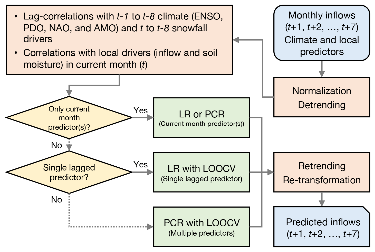
Figure 1Graphical representation of the monthly prediction (MP) model scheme. At each calendar month t, we develop seven independent models to predict monthly inflows for the next 7 months: MP1 (t+1), MP2 (t+2), …, MP7 (t+7).
3.1 Dam inflow prediction model
Seasonal streamflow forecasting approaches include physically based (mechanistic) models, such as GloFAS (a global-scale forecasting system; Emerton et al., 2018; Harrigan et al., 2020); empirical or statistical (data-based) models that leverage the relationship between large-scale climate drivers and local hydro-meteorological processes (Block, 2011; Gelati et al., 2014; Giuliani et al., 2019); and conceptual (parametric) models that integrate hydrological processes at the catchment scale (Lindström et al., 2010; Devia et al., 2015). Here, we select the second approach because of two reasons. First, the prediction horizon of most openly available global reforecasts (from a few days to 3–4 months) falls short of our preferred lead time (up to 7 months), which is needed to test the potential of realistic forecasts for a broad spectrum of reservoirs – including those characterized by slow storage dynamics. Second, reforecasts issued by global-scale forecasting systems are only available for a relatively short hindcast period (typically 2 decades; Harrigan et al., 2020), whereas the time series of globally available hydro-climatological data are significantly longer. It should be noted that these two statements may change in the near future as the boundaries of global-scale forecasting systems keep getting extended (see Sect. 5.2). For example, there already exist global reforecasts from physically based models with a prediction horizon of 7 months and hindcast periods of about 30 years (https://hypeweb.smhi.se/explore-water/forecasts/seasonal-forecasts-global/, last access: 5 May 2022).
Our long-range inflow prediction model uses principal component regression (PCR) and includes four lagged large-scale climate drivers, snowfall, and prior inflow and soil moisture conditions to predict future inflows at 735 dams. This approach is readily implemented globally and has demonstrated fair (realistic) predictive skill at 1200 streamflow stations (Lee et al., 2018). While Lee et al. (2018) predicted seasonal (3-month) streamflow averages, here we develop independent monthly prediction (MP) models for the subsequent 7 calendar months. For example, forecasts issued at the end of February include monthly inflows from March (MP1) to September (MP7).
The methodology relies on the following steps, illustrated in Fig. 1. First, we normalize (log-normalize for streamflow) and detrend all predictors and streamflow observations to avoid spurious correlation. Then, we estimate the lag correlations between future monthly inflows over the next 7 months (t+1 to t+7) and historical climate indices (t−1 to t−8), snowfall (t to t−8), and inflow and soil moisture in current month (t). Only statistically significant predictors are subsequently used to develop the MP models. If only a single (statistically significant) predictor exists, we apply a linear regression (LR) model; otherwise, we apply the PCR model to avoid possible multi-colinearities. In the PCR process, we truncate only the last principal component, which is typically associated with multi-colinearities, as suggested by Jolliffe (2002) and Wilks (2011). To select the optimal lag times of the predictors, we apply a leave-one-out cross-validation (LOOCV) scheme. Specifically, all combinations of lag times of the predictors are cross-validated; then, the optimal set of lag times is determined based on the minimum mean squared error (MSE). The models are developed with 70 % of the available data (corresponding to the period 1958–1987) and validated with the remaining data (1988–2000) so as to measure the model's independent performance over the recent period. In the validation process, we evaluate the model performance using two skill scores, namely, the mean squared error skill score (MSESS) and the Gerrity skill score (GSS) (Sect. S2 and Fig. S2). If an MP model has no statistically significant predictors or either an MSESS or GSS value lower than 0, the long-term average for that month (i.e., the climatological mean) is applied instead. The overall accuracy of the reservoir inflow predictions is assessed with the Kling–Gupta efficiency (KGE), which compares correlation, bias, and variability of the predicted and observed discharge (Gupta et al., 2009). The KGE is defined as
where r is the correlation coefficient, β the bias ratio of the mean inflow (), γ the variability ratio , μ the mean flow, CV the coefficient of variation, and s and o are two indices indicating simulated (predicted) and observed inflow values, respectively.
3.2 Reservoir operation model
3.2.1 Reservoir model
An essential component of the operating scheme is the reservoir mass balance described below:
where St is the reservoir storage at month t, Qt the inflow volume (retrieved from the WaterGAP model, as described in Sect. 2.1), Et the evaporation loss, and Rt the water released through the turbines. The evaporation loss Et is calculated by multiplying the surface area of a reservoir (at each time period t) by the potential evaporation, retrieved from the WaterGAP model. Both St and Rt are constrained by the reservoir design specifications. Specifically, the storage cannot exceed the reservoir capacity Scap (Eq. 2b), while the discharge is bounded by the water availability and capacity Rmax of the turbines (Eq. 2c). Excess water, if any, is spilled:
The hydropower production Pt (in MW) is calculated as follows:
where η is the efficiency of the turbines (assumed constant at 0.9 over the simulation period), ρ the water density (1000 kg m−3), g the gravitational acceleration (m s−2), rt the average release rate (m3 s−1) implied by the monthly release volume Rt, and ht the hydraulic head (m). The last variable is taken as the average head between time t and t+1.
3.2.2 Benchmark scheme: control rules
Our benchmark operating scheme relies on the approach proposed by Ng et al. (2017), in which the behavior of the hydropower operators is modeled as an optimal control problem. This approach builds on two main assumptions. First, the goal of the operators is to maximize hydropower production over the long term. This objective provides a tangible indication of hydropower performance, so it is commonly adopted in large-scale studies (e.g., Van Vliet et al., 2016). Second, the release decision Rt depends on the reservoir storage St, the previous period's inflow volume Qt−1, and month of year t, which is a common choice in real-world reservoir operating schemes (Hejazi et al., 2008). In other words, the approach assumes that each reservoir is operated through a unique periodic look-up table of turbine release decisions, which is generated through stochastic dynamic programming (Loucks et al., 2005; Soncini-Sessa et al., 2007). In the optimization, the inflow process is modeled with a first-order, periodic Markov chain, whose parameterization is derived from the inflow data. This means that climatology and interannual inflow variability are embedded in this operating scheme. Such schemes are more sophisticated than operating schemes relying only on storage level and time of the year (Denaro et al., 2017; Giuliani et al., 2019; Ahmad and Hossain, 2020) and are more consistent with inferred operating rules (Turner et al., 2020). A detailed validation of the operating rules – based on values of observed hydropower production in 107 countries during the period 1980–2000 – is reported in Turner et al. (2017b). The time series of all process variables (e.g., inflow, storage, release, hydropower production) obtained by the benchmark control scheme are available on HydroShare (http://www.hydroshare.org/resource/ca365ffb1a1f49df8b77e393be965fd8, last access: 5 May 2022).
3.2.3 Forecast-informed scheme
To assess the value of seasonal streamflow forecasts, we adopt an adaptive scheme based on the receding horizon principle (Bertsekas, 1976). At month t, we use a deterministic 7-month streamflow forecast to determine the value of the release decisions for the next 7 months, and then we implement only the decision Rt for the first month. At month t+1, when a new 7-month forecast becomes available, a new sequence of release decisions is determined. Each decision-making process is formulated through an optimization problem that maximizes the hydropower production over the forecast horizon while accounting for the benefits associated with the resulting storage at the end of the forecast horizon:
where Pt is the hydropower production (see Eq. 3), and X(⋅) is a function accounting for the long-term effect of the release decisions. Specifically, the function penalizes decisions that solely optimize energy production in the short term, risking water availability depletion in the long term. Following a common practice in forecast-informed schemes (Soncini-Sessa et al., 2007), we set X(⋅) equal to the benefit function obtained by the benchmark control rules, which contains information about the expected long-term hydropower production for a given storage level. Thus, the real-time information provided by the forecasts may alter decisions otherwise based solely on the benchmark scheme. As our inflow forecast model gives a deterministic 7-month forecast, the optimization problem is solved at each time step using deterministic dynamic programming (Turner et al., 2017a).
The scheme is implemented using both “perfect” and realistic forecasts. Both benchmark and forecast-informed schemes are simulated over the period 1958–2000. The storage of all reservoirs is initialized at full capacity at the beginning of each simulation. During the simulation, all release decisions are constrained to satisfy downstream environmental flow requirements, calculated using the variable monthly flow method (Pastor et al., 2014). The implementation of stochastic and deterministic dynamic programming (for control rules and forecast-informed scheme, respectively) requires us to discretize the values of storage and release. In particular, storage is discretized into 500 uniform values, while release is discretized into 20 uniform values between 0 and Rmax (Turner et al., 2017a). For each reservoir, we check that the ratio between Rmax and number of discretized values (for release) is larger than the ratio between Scap and number of discretized values (for storage), thereby ensuring that different release decisions lead to different storage levels when transitioning between two simulation time steps. For stochastic dynamic programming, we also discretize inflow according to the bounding quantiles of 1.00, 0.95, 0.7125, 0.4750, 0.2375, and 0.00 (as recommended by Stedinger et al., 1984). The likelihood of each flow class is computed for each month using inflow data from the WaterGAP model. All experiments are carried out with the R package reservoir (Turner and Galelli, 2016).
3.2.4 Considering additional operating objectives and finer temporal scales
Of the 735 headwater dams in the database, 174 dams are also operated for flood control purposes. For these dams, we penalize spill to account for flood control and formulate the optimization objective as follows (in both benchmark and forecast-informed schemes):
where w1 and w2 are the weights associated with the flood control and hydropower objectives (set to 0.5 here), p95(Q) the 95th percentile of the inflow time series Q, and P the dam installed hydropower capacity (in MW). Clearly, additional objectives may influence hydraulic head or the release trajectory, thereby affecting hydropower production (Zeng et al., 2017).
A second modification of the reservoir operation model concerns the monthly decision-making time step, which may not be suitable for reservoirs with small storage capacity relative to inflow (time-to-fill value). We therefore identify a group of 94 reservoirs for which the time-to-fill value is shorter than 2 months, and we adopt for this group only a weekly time step. Since the inflow forecasts have a monthly resolution, we disaggregate each forecast into four values using the k-nearest-neighbors algorithm (Nowak et al., 2010). Further details are reported in Sect. S3.
3.3 Reservoir performance evaluation
It is reasonable to hypothesize that the value of seasonal streamflow forecasts – here measured in terms of hydropower production – depends not only on predictive skill but also on reservoir characteristics. For example, a reservoir constrained by small turbine capacity may perform adequately utilizing control rules alone, as storage is sufficient to buffer inflow variability. We are thus interested in quantifying forecast value as well as understanding how value varies as a function of both skill and reservoir characteristics. This leads us to the following performance metrics.
3.3.1 Impact of design characteristics on perfect forecast-based operations
Initially excluding the effect of actual forecast skill, the following performance metric represents the expected improvement from perfect forecast-informed operations as compared to control-rules-based operations:
where HPF and Hctrl represent the total hydropower production (for the period 1958–2000) obtained with perfect forecast-informed operations and control rules, respectively. A value equal to zero indicates that the control rules are comparable to the (perfect) forecast-informed operations, whereas a positive value suggests that forecast-informed operations could be beneficial. Even though some dams are operated with an additional flood control objective, we use the same measure for all dams so as to ensure a consistent comparison of forecast value.
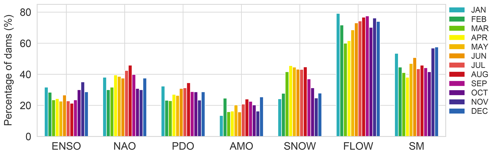
Figure 2Percentage of dams whose inflow is significantly correlated with lagged predictors (ENSO, NAO, PDO, AMO, and snowfall) and 1-month ahead predictors (inflow and soil moisture) in each calendar month.
To understand how reservoir characteristics may influence benefits attained with perfect forecasts, we proceed in two steps. First, we label each dam as case (also referred to as success) if it has the desired property of an IPF value larger than the mean value of IPF across all dams. Otherwise, the dam is labeled as non-case. (As this labeling is rather arbitrary, we later assess the sensitivity of our analysis to changes in the threshold.) Second, we explain the likelihood of achieving success through a logistic regression model in which the probability of the binary response variable taking a particular value is a function of the predictor variables. We consider two predictors, namely, (1) the ratio of reservoir storage capacity to the mean monthly inflow (xfill, measured in months) and (2) the ratio of maximum reservoir depth to maximum hydraulic head (xdepth). The second predictor varies between 0 and 1 and indicates the extent to which hydraulic head is dependent on the depth of the reservoir. The logistic regression model is cross-validated with a 10-fold cross-validation scheme and evaluated using two metrics: accuracy and Cohen's kappa (McHugh, 2012). Accuracy is the ratio of correctly predicted observations (true positives and true negatives) to the total number of observations. Cohen's kappa is an adjusted accuracy score that accounts for the possibility of correct predictions occurring by chance. The modeling exercise is carried out with the R package caret. For additional details, please refer to Sect. S4 and Tables S1–S3 in the Supplement.
3.3.2 Impact of forecast skill and design characteristics on realistic forecast-based operations
Integrating realistic forecasts in lieu of perfect forecast information, we introduce the following performance metric:
where HDF represents the total hydropower production (for the period 1958–2000) obtained using realistic forecast-informed operations. IDF is then combined with IPF to calculate the performance metric I that quantifies the potential improvement between realistic and perfect forecast-informed operations:
A value of I equal to 1 indicates that benefits from the actual forecasts equal those utilizing perfect forecasts. A value of 0 denotes performance equivalent to applying the control rules only, while a negative value implies that the forecast-informed scheme is inferior to the control rules. We calculate this metric only for the subset of dams achieving a value of IPF greater than the mean value of IPF to better understand if the benefits modeled with perfect forecasts may be attainable with realistic forecasts.
To explain how the metric I varies, we use a linear regression model accounting for both forecast skill and reservoir characteristics. The predictor characterizing the forecast skill is xMdAPE, which is the median absolute percentage error of the forecast and is used in place of KGE as it shows a higher correlation with I. (While KGE gives a broad view of the forecast skill by comparing correlation, mean, and standard deviation of the predicted and observed inflows, MdAPE accounts for the forecast error at every time step of the inflow time series. This may make MdAPE a more suitable predictor, as the error at each time step affects the release decisions and, ultimately, hydropower production.) The second predictor is xexceed, the fraction of time that inflow exceeds the maximum turbine release rate. For more details on the choice of predictors, please refer to Sect. S5 and Tables S4–S6.
In this section, we first present the accuracy of the inflow prediction models (Sect. 4.1) and performance of the forecast-informed schemes (Sect. 4.2). Then, we quantify the extent to which reservoir design characteristics and forecast skill affect the value of seasonal forecasts (Sect. 4.3). Lastly, we classify all dams according to their potential to benefit from forecasts, and we identify key geographical regions that may benefit the most from forecasts (Sect. 4.4).
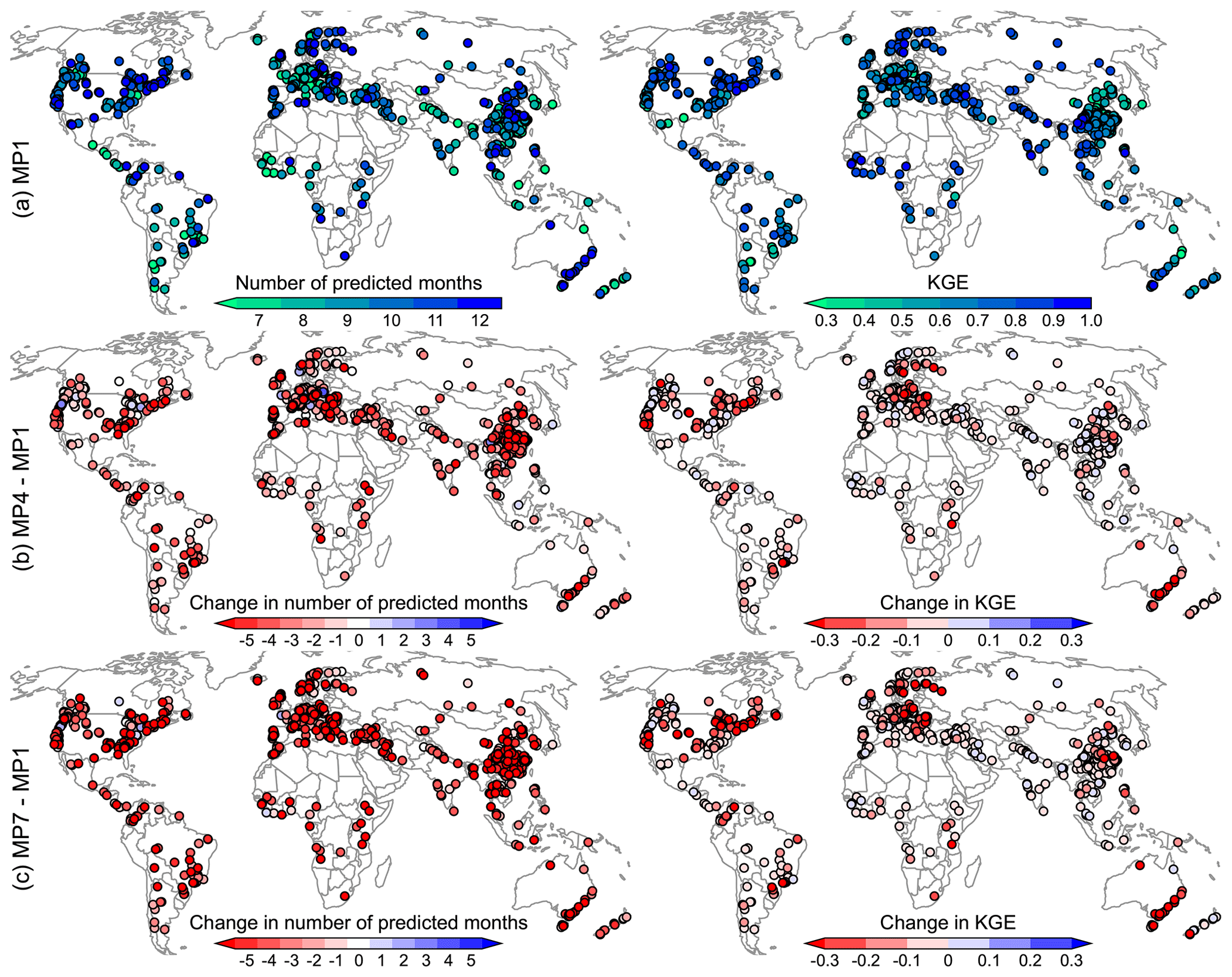
Figure 3Number of months in which a predictive model is developed (left) and corresponding KGE (right). Taking a model with a lead-time of 1 month (MP1) as reference (a), we report the difference between MP1 and MP4 (b) and MP1 and MP7 (c).
4.1 Potential predictors and accuracy
As shown in Fig. 2, reservoir inflow exhibits significant correlation with climate and local drivers (potential predictors). Yet, this relationship changes across the annual cycle. Evaluating months when a higher percentage of dams is significantly correlated with predictors, some well-known climatic teleconnections can be observed – e.g., ENSO and winter–spring streamflow in North America and Europe, NAO and spring–summer peak flows in the northern extratropical regions, and PDO and summer streamflow in southeastern North America and central South America (Fig. S3). On average, 27 %, 37 %, 28 %, 20 %, and 36 % of the reservoir catchments are significantly correlated with ENSO, NAO, PDO, AMO, and snowfall, respectively. Additionally, and not surprisingly, inflow for most dams (72 %) exhibits significant 1-month lead autocorrelation. An exception is represented by some dams during the period March-April, especially in areas with minimal baseflow (Figs. 2 and S3). Soil moisture at a 1-month lead is statistically significantly correlated with inflow at 47 % of dams across all months with a seasonality similar to inflow.
Reservoir inflow and climatic predictors are often (significantly) correlated across several lead months. In these cases, climate predictors are very likely to be included in multiple MP models for various leads, although the correlation may decrease with longer lead-time. When a climate predictor is significantly correlated with reservoir inflow at a 1-month lag (MP1), 74 % and 38 % of the time it is also included at the 4-month lag (MP4) and 7-month lag (MP7), respectively. Snowfall has a similar retention rate. However, and as expected, autocorrelation in inflow and soil moisture drops more precipitously with longer lead; only 53 % (28 %) of the time, when lagged inflow and soil moisture are included as predictors in MP1, they are also included in MP4 (MP7). Globally, an average of 2.7, 1.7, and 0.9 predictors are included in the MP1, MP4, and MP7 models, respectively. In very few cases, the number of predictors increases with longer lead-time. For months when no potential predictors are identified, or either MSESS or GSS is less than zero, the long-term mean inflow for that month is used.
Across the annual cycle, the average number of months in which at least one predictor is included (and thus a predictive model developed) is equal to 8.3 months (MP1), 6 months (MP4), and 4.2 months (MP7) (see Fig. 3). As noted previously, a lack of long-lead inflow autocorrelation is predominantly responsible for this drop (and thus for increased reliance on climatology-based forecasts). Prediction accuracy also decreases with lead-time; average KGE values are 0.64 and 0.56 for MP1 and MP7, respectively (Fig. 3). Given that prediction accuracy generally declines with lead time, the highest KGE scores across all MP models are associated with MP1 for 68 % of the dams. For the remaining models, the highest prediction accuracy is recorded for 5 % (2 %) of dams in the MP4 (MP7) models, emphasizing that skillful forecasts at longer leads do exist, such as in Europe or northwestern and southeastern USA (Fig. 3b and c). As for the geographical distribution of KGE, we find relatively high KGE scores in several regions, including North America, eastern South America, Europe, and some regions in western Africa and Asia, where inflows correlate with most of the considered predictors (Figs. 3 and S3). For some regions that often exhibit skillful precipitation predictability based on well-known teleconnections and hydroclimate mechanisms, such as northwestern South America, East Africa, and southeastern Africa (Lee et al., 2018), this is not readily apparent on the KGE maps (Fig. 3), owing primarily to the regions' low dam density and thus a small sample size.
For all MP models, the KGE has an average value of about 0.56, which is regarded as a fair skill score outcome. While uniquely tailored forecasts could be produced for each dam considering more local influences, the current prediction approach performs well globally and reflects achievable long-range inflow predictions. Considering the superior performance of the MP1 model, the forecast skill of MP1 only is retained to represent the overall forecast skill in the following analyses. (For an additional analysis concerning the relationship between dam performance and the speed with which forecast skill decreases, please refer to Sect. S6 and Fig. S4.)
4.2 Performance of forecast-informed operations
The expected performance of perfect and realistic forecast-informed operations is notably different across the 735 hydropower dams (Fig. 4). With perfect forecast-informed operations (Fig. 4a), we observe a substantial increase in hydropower production with respect to the baseline control rules. Specifically, 94 % of dams exhibit a positive value of the performance metric IPF; mean improvement is 4.7 % and maximum improvement is 60 %. For the small number of dams that do not benefit from perfect forecasts, the value of IPF does not drop below −1.7 %. Small negative values of IPF may be a result of the discretization needed by dynamic programming to optimize the release sequence (Eq. 4), hence allowing control rules to outperform perfect forecast-informed operations. (Recall that storage and release are discretized into 500 and 20 values, respectively: when the storage level falls between two discrete levels, the closer level is selected and the optimum release decision for that discrete level is implemented. This decision may sometimes be suboptimal, giving rise to negative values of IPF.) Considering all dams collectively, an additional 24 TWh yr−1 of hydroelectricity is generated when adopting the perfect forecast-informed approach in lieu of baseline control rules. This is equivalent to 0.57 % of the 4200 TWh of hydropower globally generated in 2018 (note that the headwater dams used here represent 10 % of the world's installed capacity) (IHA, 2019). Such modest global benefit and large range of individual benefits suggest that the forecast value is highly dependent on the reservoir characteristics (see Sect. 4.3).
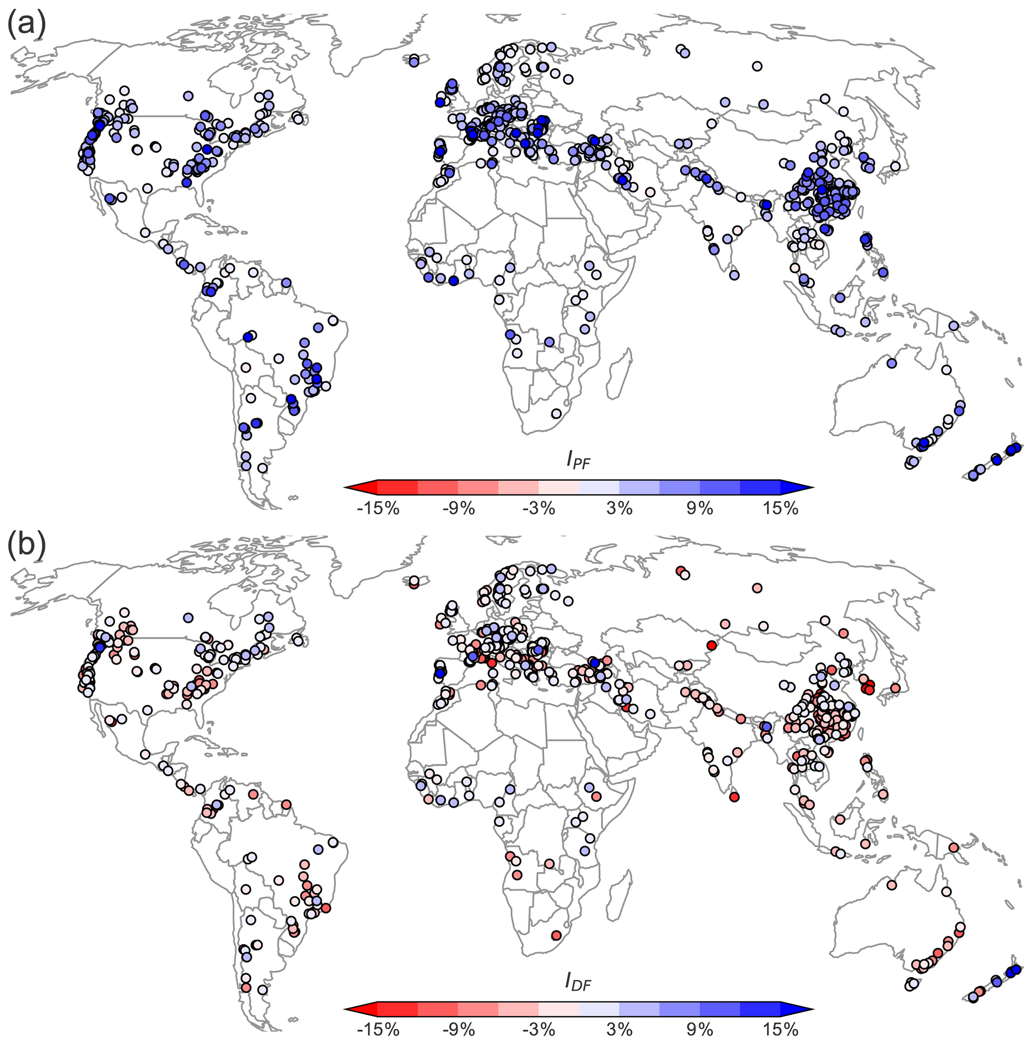
Figure 4Improvements in hydropower production using perfect (a) and realistic (b) forecasts. The terms IPF and IDF indicate the relative improvement in hydropower production (with respect to the basic control rules) provided by perfect and realistic forecasts. Nearly all dams are able to benefit from perfect forecasts, but only 25 % of dams benefits from realistic forecasts.
When realistic forecast-informed operations are adopted (Fig. 4b), a smaller number of dams exhibit increased hydropower production. IDF ranges from −24 % to 28 %, with 25 % of dams showing a positive value of IDF. The 184 dams with positive IDF values show an average improvement of 2.3 % and collectively contribute an additional 1.7 TWh yr−1 in hydropower production, which is 7 % of the 24 TWh of additional hydropower obtainable from perfect forecasts. This decline in performance is expected, as realistic forecasts introduce a non-negligible prediction error. Yet, it should also be noted that less than 20 % of dams have a KGE value below 0.5, whereas a disproportionately larger number of dams exhibit a negative IDF value. This suggests that for a large number of dams control-rules-based operations are superior to realistic forecast-informed operations. For dams with poor IDF and high KGE, two features are noteworthy: first, KGE may not fully capture the relationship between forecast skill and value, and, second, reservoir characteristics are an important factor influencing the value of realistic forecasts.
4.3 Evaluation of prediction accuracy and reservoir characteristics
To understand the extent to which reservoir characteristics may modulate the value of seasonal forecasts, we identify a logistic regression model that explains the likelihood of achieving success with perfect forecasts (IPF larger than 4.7 %, i.e., the mean value of IPF across all dams) as a function of two predictors, xfill (the ratio of reservoir storage capacity to the mean monthly inflow) and xdepth (the ratio of maximum reservoir depth to maximum hydraulic head). A 10-fold cross-validation yields a model accuracy and kappa statistic of 0.785 and 0.535, respectively. (Note that the percentage of dams labeled as cases and non-cases is equal to 37 % and 63 %, respectively.)
As illustrated in Fig. 5 and Table 1, both predictors influence the probability of achieving success. For xfill values exceeding 10 months, dams are highly unlikely to benefit substantially from seasonal forecasts. This suggests that a large storage capacity effectively acts as a buffer against inflow uncertainty. Hence, both control rules and perfect forecast-informed operations tend to attain similar performance. We also observe that some of the smaller dams (xfill<2) fail to attain increased hydropower production even though they are predicted to do so (red triangles in the blue shaded region; Fig. 5). This is because weekly operations decrease IPF for some of these dams to below the mean IPF, turning them from cases (if operated on a monthly basis) into non-cases. This suggests that more frequent release decisions may reduce forecast value, since the benchmark operating rules have more opportunities to adjust release decisions. For smaller dams, xdepth becomes a critical factor. High values of xdepth indicate that the hydraulic head is highly dependent on the reservoir depth, which is in turn dependent on current and near-future inflows for dams that cannot accumulate large inflow volumes. Thus, forecast-informed operations become crucial to maintain a high hydraulic head and maximize hydropower production. For hydropower dams that have a low value of xdepth, a high hydraulic head is maintained even when storage is low, thereby minimizing the utility of forecasts. These are systems relying on waterfalls, or hilly terrains, to divert part of the water and gain hydraulic head.
Table 1Coefficients of logistic regression to predict if IPF>4.7 %. The term “Estimate” represents the increase in log-odds of a dam being classified as case (or success) per unit increase in the value of the predictors.
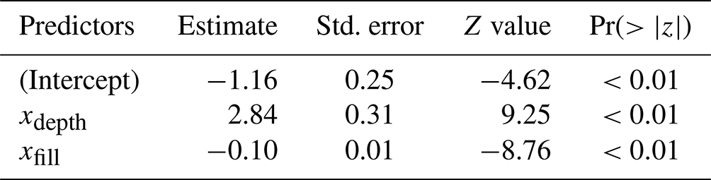

Figure 5Probability of success estimated using a logistic regression model with predictors xdepth and xfill (in log scale). Red corresponds to a probability of success equal to zero, meaning that the dam is likely to do well with the control rules. Blue represents a probability of success equal to 1, meaning that a dam is likely to benefit from forecast-informed operations. Each point in the plot represents one of the 735 dams. Blue circles represent dams labeled as cases (or success) (IPF>4.7 %) and red triangles represent non-cases. The size of the blue circles represents the value of IPF. All red triangles have the same size. Dams below the dashed line (xfill=2) are operated with a weekly time step. Dams with low values of xfill (small storage capacity relative to inflow rate) and high xdepth (lacking a natural waterfall) are more likely to benefit from forecast-informed operations.
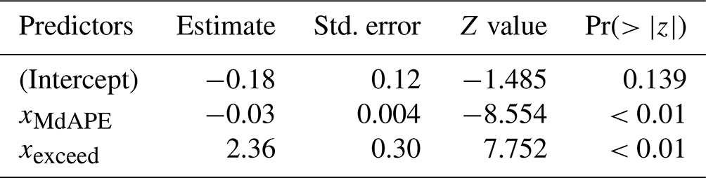
Considering only the subset of 269 dams that have an IPF value larger than 4.7 %, we apply a linear regression model to estimate the performance metric I. This time, the predictors include xMdAPE (median absolute percentage error of forecast inflows) and xexceed (the fraction of time that inflow exceeds the maximum turbine release rate). The linear regression model has an adjusted R2 of 0.31, which can be increased further by considering other variables related to inflow variability and hydraulic head. The reader is referred to Tables S4–S6 for more complex models that include additional predictors.
The results are presented in Table 2 and illustrated in Fig. 6. As expected, higher forecast skill (lower xMdAPE) increases the potential benefits realized by the realistic forecasts; a 1 % decrease in xMdAPE increases I by 0.03. Reservoir characteristics can play an important role, as certain configurations allow dams and hydropower production to benefit from realistic forecasts. Specifically, we find that dams in which inflow frequently exceeds maximum turbine release (large values of xexceed) are more likely to benefit from forecast-informed operations – even when forecasts are not very accurate, as shown by the diagonal divide in Fig. 6. This is predominantly a result of both forecast and observed inflow frequently exceeding the maximum turbine release rate, a situation in which the release decision would be the same regardless, so consequently inaccurate forecasts do not penalize hydropower production.
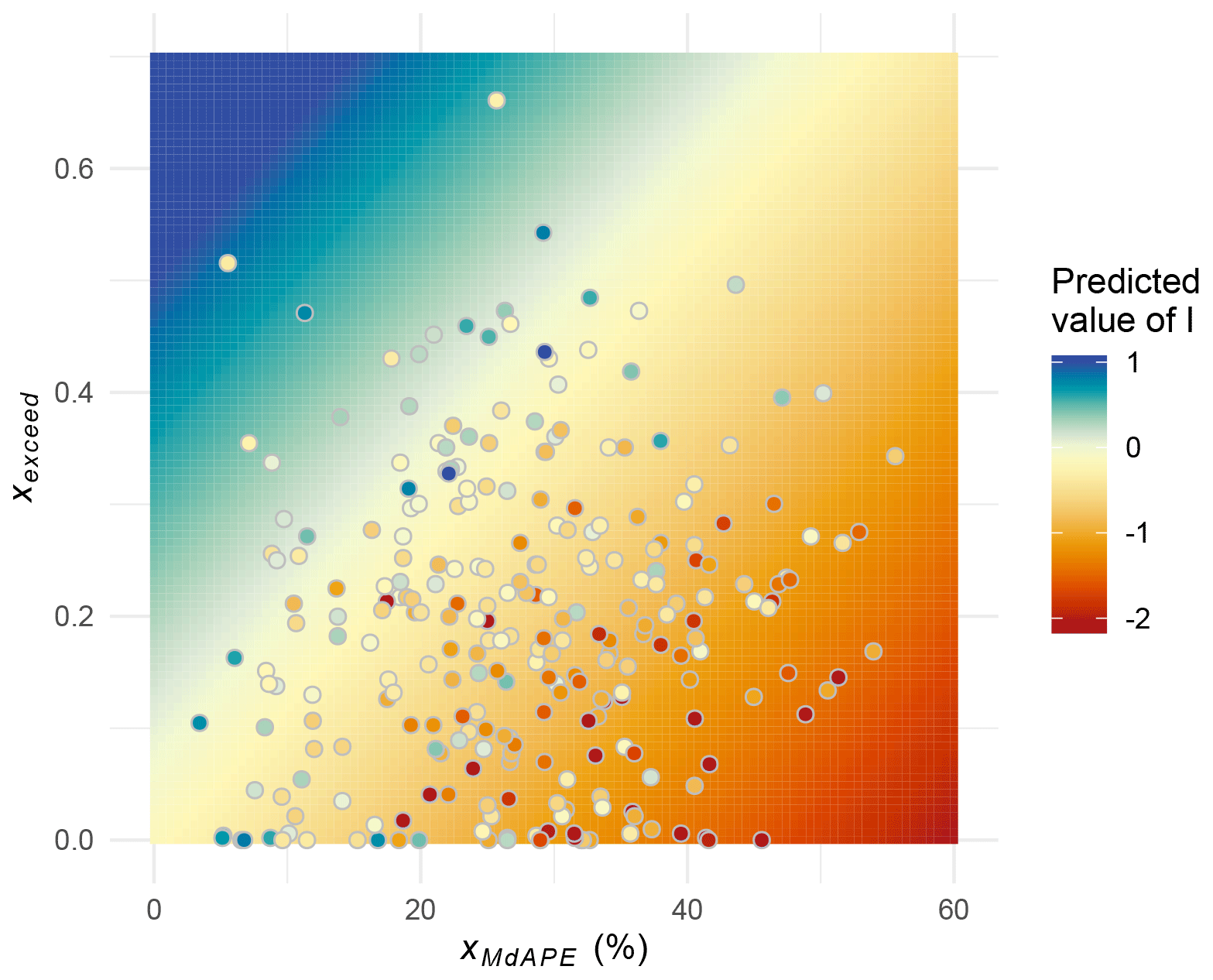
Figure 6Potential benefits realized by realistic forecast (I) predicted using linear regression with predictors xexceed and the median absolute percentage error (xMdAPE). Red corresponds to negative values of I, meaning that the performance of realistic forecasts is worse than the one attained by control rules. Blue corresponds to positive values of I, meaning that realistic forecasts outperform control rules. Each point corresponds to one of the 269 dams with IPF>4.7 %. The corresponding color represents the value of I attained via simulation with the reservoir operation model. Dams with accurate forecasts and high values of xexceed (inflow frequently exceeds maximum turbine release) tend to have greater hydropower benefits realized from realistic forecasts.
4.4 A classification of hydropower dams
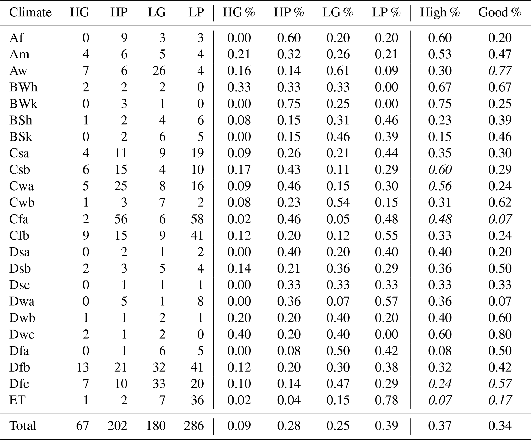
Building on the results described above, we divide the dams into four groups on the basis of their potential to benefit from perfect forecast-informed operations (high potential if IPF>4.7 % and low potential otherwise) and forecast skill (good forecast if xMdAPE<20 % and poor forecast otherwise). The cutoff value for IPF is inferred from the previous analysis (logistic regression model), while the cutoff for xMdAPE divides the 735 dams into two groups of one-third (good forecast) and two-thirds (poor forecast) of the observations. The distribution of the dams across the four groups (and Köppen–Geiger climate zones) is reported in Table 3. Two groups of dams of particular interest include (1) dams that fall in regions expressing strong forecast accuracy and have the potential to reap benefits from forecast-informed operations (9 % of the total number of reservoirs) and (2) dams with a strong potential to benefit from forecast-informed operations but lack forecast accuracy (28 %). As discussed in Sect. 5, this lack of forecast accuracy could be readily addressed by adopting more sophisticated forecast models or further leveraging local predictors.
Table 3Distribution of dams across climate zones. In columns 2–9, H and L indicate the potential (high/low) of benefiting of forecasts, while G and P indicate the quality (good/poor) of realistic forecast. Columns 2–5 (6–9) are the number (percentages) of dams in each group. The last two columns report the percentages of dams with high potential and good forecast, respectively. Values reported in italics indicate whether the observed frequency is statistically different from the expected frequency (global average in the final row) (p<0.05 using χ2 test).
As described in Sect. 4.3, the potential of a dam to benefit from forecasts is largely dependent on its design specifications, which present comparable values in areas with similar orography and design practices. Forecast skill, on the other hand, is largely dependent on climate teleconnections, which tend to present regional patterns. Further, considering these factors coincidentally is also insightful. Figure 7 illustrates the distribution of the four possible groups of dams across the thirty climate zones of the Köppen–Geiger climate classification system. We notice a few interesting patterns. First, dams with high potential but lacking accurate forecasts (panel (a), red triangles) are often found in humid subtropical climate zones (Cwa, Cfa), particularly in the southeast regions of Australia, China, USA, and South America. The trend is also true – but not statistically significant – for dams in Southeast Asia (tropical rainforest, Af) and US Pacific Northwest (warm summer Mediterranean, Csb). Second, dams with good forecasts (panels (a) and (b), blue triangles) are mostly located in the tropical savanna climate zone (Aw, mainland Southeast Asia, India, Brazil, and western Africa) and subarctic climate zone (Dfc, Canada, Russia, northeastern Europe). While the majority of these dams have poor to fair potential, which can be attributed to relatively large time-to-fill values, the remaining dams with characteristics conducive for forecast-informed operations can readily benefit from including climate signals into their forecast models. This also applies to dams along the US–Canadian border. These dams are located in a humid continental climate zone (Dfb), whose statistical significance for high forecast accuracy has been masked by differences in performance between dams located in Europe and North America. Third, dams with low potential and poor forecasts are primarily found in Europe and east Asia (panel (b), red triangles). This trend is significant (p<0.05) for dams in the Alps (alpine climate, ET), in particular for dams that are characterized by large time-to-fill values and small reservoir depth to maximum hydraulic head ratios. This classification of dams based on climate zones, potential to benefit from perfect forecast-informed operations, and forecast skill is complemented by an additional analysis informed by the Hydrological Climate Classification (Knoben et al., 2018), which also accounts for hydroclimate characteristics. Please refer to Sect. S7 and Fig. S5.

Figure 7Distribution of dams across climate zones based on their potential to benefit from perfects forecasts. The top (a) and bottom (b) panels represent dams with “high potential” (IPF>4.7 %) and “low potential” (IPF≤4.7 %), respectively, while “good forecast” and “poor forecast” represent dams with MdAPE less than or greater than 20 %, respectively.
5.1 Implications for planning and management of hydropower projects
In this study, we examine the relationship between seasonal streamflow forecasts and global hydropower production, accounting for the influence of reservoir characteristics. Specifically, we develop seasonal inflow forecasts for 735 headwater dams based on lagged global and local hydroclimatic variables. The forecasts exhibit fair skill globally, but higher skill in several regions, including the northern extratropical regions and the areas characterized by tropical savanna climate (e.g., mainland Southeast Asia, eastern South America, and western Africa). In agreement with earlier work, our forecasts exhibit well-known teleconnections, such as NAO influencing spring–summer peak flow in the northern extratropical regions (Lee et al., 2018), ENSO influencing streamflow in Southeast Asia (Sankarasubramanian et al., 2009; Räsänen and Kummu, 2013), and ENSO / PDO influencing winter–spring streamflow in the Pacific Northwest (Hamlet et al., 2002; Voisin et al., 2006).
We then illustrate the relationship between forecast skill, value, and reservoir characteristics by adopting forecasts in the reservoir operations model. While 94 % of dams considered could benefit from perfect forecasts, only 25 % demonstrate improvements when using our realistic forecasts – a fairly low percentage if we consider the forecast skill achieved globally. This highlights the fundamental role of reservoir characteristics in shaping the relationship between forecast skill and value. Key design specifications include time-to-fill value, which is a characteristic identified by other recent studies (Anghileri et al., 2016; Turner et al., 2017a; Yang et al., 2020); hydraulic head, which is largely dependent on reservoir depth; and the frequency of inflows exceeding maximum turbine release rates, which is a design specification that allows operators to work with a larger margin of forecast error during high-inflow periods. It is worth emphasizing here that these results are not intended to provide site-specific operational guidelines, but they do represent a first, qualitative step toward determining the potential benefit of seasonal streamflow forecasts for hydropower operators. The relationships identified here could be used, for example, to understand forecast potential for a given reservoir or to characterize the interplay between climatology, hydrology, and dam characteristics in a large region of interest.
By combining information on reservoir characteristics, forecast skill, and climatic zones, we identify large regions in which dams would benefit the most from forecast application. One such group consists of dams with a strong potential to benefit from forecast-informed operations and that possess good forecast accuracy. In particular, for the tropical savanna and subarctic climate, we observe teleconnections that result in higher forecast accuracy. Dams with favorable characteristics in these regions can gain additional benefits from integrating large-scale climate signals within forecast models. Another interesting group consists of dams that may benefit from forecast-informed operations but lack adequate forecast accuracy. Such dams are located in maritime Southeast Asia, the Pacific Northwest, and the humid subtropical climate of the southeast regions of Australia, China, USA, and South America. These are areas in which watershed-specific analyses may bring immediate benefits to hydropower operators. Such analyses will likely require more nuanced hydro-climatological data than those adopted here – from observed precipitation in the upstream catchment (Denaro et al., 2017) to temperature and precipitation data forecasted by numerical weather prediction models (Ahmad and Hossain, 2020).
Finally, it is worth noting that the implications of our study go beyond existing reservoirs: dam planning over large scales may also benefit from these findings. For example, untapped hydropower potential (Zhou et al., 2015; Hoes et al., 2017) and seasonal streamflow predictability could be evaluated to derive some first, qualitative, conclusions on expected reservoir characteristics and performance. A case in point is run-of-the-river dams: these systems have a short time-to-fill characteristic and are therefore suitable for implementing forecast-informed reservoir sizing and operations (Bertoni et al., 2021). Conversely, if new dams are constructed in areas known to lack forecast skill or monitoring systems, then a larger storage capacity may be justifiable for dams operating with basic control rules.
5.2 Limitations and opportunities
Like any other global study, the large spatial domain requires building on a number of assumptions that must be properly contextualized. First, we assume that the goal of dam operators is to maximize hydropower production over the long term (in addition to providing flood control). While this objective provides a tangible indication of forecast value, it may not be fully representative of the local conditions encountered by operators. For example, operators may be interested to maximize revenue (Anghileri et al., 2018), supply the bulk of power to the grid (Zambon et al., 2012), or complement the generation of other renewable energy sources (Graabak et al., 2019). To account explicitly for these aspects, one needs to model the role that dams play in the power market, as recently done for the western USA (Voisin et al., 2020), England (Byers et al., 2020), or the Greater Mekong (Chowdhury et al., 2020, 2021). With these models, one could also infer the willingness to pay for improved streamflow forecasts based on the economic value derived from their use (Arnal et al., 2016).
Second, release decisions at individual dams may be affected by joint operations between multiple reservoirs. The analysis could thus be better supported by more accurate data and tailored hydrological models surpassing those adopted here. Importantly, these data could include qualitative or quantitative forecasts. Although precipitation and streamflow predictions are not used consistently across the world (Adams and Pagano, 2016), medium- to long-range forecasts are increasingly being adopted by water utilities – as recently shown by Turner et al. (2020) for 300 dams in the conterminous United States. Access to observed and inferred release decisions could thus help researchers provide a more robust and nuanced estimate of forecast value. Accurate data and tailored hydrological models could also help quantify the extent to which operators may benefit from predicting other variables than the average inflow, such as the inflow peak over a given horizon (Bertoni et al., 2021).
Finally, the investigation of alternative forecast approaches may be warranted. In particular, our deterministic long-range forecasts could be replaced by probabilistic ones, based, for example, on ensemble dynamical forecasts or statistical models including a stochastic representation of the residuals. By adopting probabilistic forecasts, one could represent additional operational aspects, such as the capacity of hydropower dam managers to inform their decisions based on probabilistic information. Such an extension to our study could possibly uncover greater potential for improving dam operations (Zhao et al., 2011) and allow for a more nuanced quantification of forecast value. When considering the forecast system, it is also important to note that regional- and global-scale forecasting systems are gaining momentum (Kirtman et al., 2014; Emerton et al., 2018), showing skillful forecasts over large spatial domains and long prediction horizons (Arnal et al., 2018; Towner et al., 2019), and this may justify investigation. Importantly, such approaches may not be limited to headwater dams, as long as the underpinning hydrological model (coupled with seasonal forecasts) includes a realistic representation of water management decisions (Pechlivanidis et al., 2020).
This analysis expands the existing body of knowledge on the relationship between forecast skill, value, and reservoir design for the hydropower sector. As expected, a positive relation between skill and value exists; however, we also demonstrate that value is strongly modulated by reservoir characteristics. The two extreme cases are represented by dams that can be profitable with little regard for forecast accuracy and dams that do not appear to benefit from seasonal streamflow forecasts. Considering reservoir characteristics and forecast skill together, we identify regions with high potential to benefit from forecast-informed operations whether forecast accuracy is good or poor. Research that integrates these findings with hydrological-electricity models to quantify economic benefits is warranted. Specifically, this may reflect the willingness to pay for improved forecast models. Such an assessment could provide guidance and insight for large-scale hydropower planning and management, particularly as energy systems become more interconnected.
The code used to conduct all analyses is available by contacting the authors. All simulations results are available on HydroShare at https://doi.org/10.4211/hs.ca365ffb1a1f49df8b77e393be965fd8 (Lee et al., 2022).
The supplement related to this article is available online at: https://doi.org/10.5194/hess-26-2431-2022-supplement.
DL, JYN, SG, and PB contributed to the conceptualization of this work. The data processing, analyses, and visualization were carried out by DL and JYN. The first draft was prepared by DL, JYN, and SG. All authors reviewed and edited the final draft.
The contact author has declared that neither they nor their co-authors have any competing interests.
Publisher's note: Copernicus Publications remains neutral with regard to jurisdictional claims in published maps and institutional affiliations.
This research has been supported by the Ministry of Education – Singapore (grant no. MOE2017-T2-1-143).
This paper was edited by Micha Werner and reviewed by two anonymous referees.
Adams, T. E. and Pagano, T. C.: Flood forecasting: A global perspective, Academic Press, ISBN 13 9780128018842, 2016. a
Ahmad, S. K. and Hossain, F.: A generic data-driven technique for forecasting of reservoir inflow: Application for hydropower maximization, Environ. Modell. Softw., 119, 147–165, 2019. a
Ahmad, S. K. and Hossain, F.: Forecast-informed hydropower optimization at long and short-time scales for a multiple dam network, J. Renew. Sustain. Ener., 12, 014501, https://doi.org/10.1063/1.5124097, 2020. a, b
Alcamo, J., Döll, P., Henrichs, T., Kaspar, F., Lehner, B., Rösch, T., and Siebert, S.: Development and testing of the WaterGAP 2 global model of water use and availability, Hydrolog. Sci. J., 48, 317–337, 2003. a
Anghileri, D., Voisin, N., Castelletti, A., Pianosi, F., Nijssen, B., and Lettenmaier, D. P.: Value of long-term streamflow forecasts to reservoir operations for water supply in snow-dominated river catchments, Water Resour. Res., 52, 4209–4225, 2016. a, b
Anghileri, D., Castelletti, A., and Burlando, P.: Alpine Hydropower in the Decline of the Nuclear Era: Trade-Off between Revenue and Production in the Swiss Alps, J. Water Res. Plan. Man., 144, 04018037, https://doi.org/10.1061/(ASCE)WR.1943-5452.0000944, 2018. a
Arnal, L., Ramos, M.-H., Coughlan de Perez, E., Cloke, H. L., Stephens, E., Wetterhall, F., van Andel, S. J., and Pappenberger, F.: Willingness-to-pay for a probabilistic flood forecast: a risk-based decision-making game, Hydrol. Earth Syst. Sci., 20, 3109–3128, https://doi.org/10.5194/hess-20-3109-2016, 2016. a
Arnal, L., Cloke, H. L., Stephens, E., Wetterhall, F., Prudhomme, C., Neumann, J., Krzeminski, B., and Pappenberger, F.: Skilful seasonal forecasts of streamflow over Europe?, Hydrol. Earth Syst. Sci., 22, 2057–2072, https://doi.org/10.5194/hess-22-2057-2018, 2018. a
Bertoni, F., Giuliani, M., Castelletti, A., and Reed, P.: Designing with Information Feedbacks: Forecast Informed Reservoir Sizing and Operation, Water Resour. Res., 57, e2020WR028112, https://doi.org/10.1029/2020WR028112, 2021. a, b, c
Bertsekas, D.: Dynamic Programming and Stochastic Control, Academic Press, New York, New York, ISBN 13 9780120932504, 1976. a
Block, P.: Tailoring seasonal climate forecasts for hydropower operations, Hydrol. Earth Syst. Sci., 15, 1355–1368, https://doi.org/10.5194/hess-15-1355-2011, 2011. a, b
Byers, E. A., Coxon, G., Freer, J., and Hall, J. W.: Drought and climate change impacts on cooling water shortages and electricity prices in Great Britain, Nat. Commun., 11, 1–12, 2020. a
Chowdhury, A. K., Dang, T. D., Bagchi, A., and Galelli, S.: Expected Benefits of Laos' Hydropower Development Curbed by Hydroclimatic Variability and Limited Transmission Capacity: Opportunities to Reform, J. Water Res. Plan. Man., 146, 05020019, https://doi.org/10.1061/(ASCE)WR.1943-5452.0001279, 2020. a
Chowdhury, K. A., Dang, T. D., Nguyen, H. T., Koh, R., and Galelli, S.: The Greater Mekong's climate-water-energy nexus: how ENSO-triggered regional droughts affect power supply and CO2 emissions, Earths Future, 9, e2020EF001814, https://doi.org/10.1029/2020EF001814, 2021. a
Crochemore, L., Ramos, M.-H., and Pechlivanidis, I.: Can continental models convey useful seasonal hydrologic information at the catchment scale?, Water Resour. Res., 56, e2019WR025700, https://doi.org/10.1029/2019WR025700, 2020. a
De Felice, M., Dubus, L., Suckling, E., and Troccoli, A.: The impact of the North Atlantic Oscillation on European hydro-power generation, https://doi.org/10.31223/osf.io/8sntx, 2018. a
Denaro, S., Anghileri, D., Giuliani, M., and Castelletti, A.: Informing the operations of water reservoirs over multiple temporal scales by direct use of hydro-meteorological data, Adv. Water Resour., 103, 51–63, 2017. a, b
Devia, G. K., Ganasri, B. P., and Dwarakish, G. S.: A review on hydrological models, Aquat. Pr., 4, 1001–1007, 2015. a
Döll, P. and Lehner, B.: Validation of a new global 30 min drainage direction map, J. Hydrol., 258, 214–231, 2002. a
Döll, P., Fiedler, K., and Zhang, J.: Global-scale analysis of river flow alterations due to water withdrawals and reservoirs, Hydrol. Earth Syst. Sci., 13, 2413–2432, https://doi.org/10.5194/hess-13-2413-2009, 2009. a
Emerton, R., Zsoter, E., Arnal, L., Cloke, H. L., Muraro, D., Prudhomme, C., Stephens, E. M., Salamon, P., and Pappenberger, F.: Developing a global operational seasonal hydro-meteorological forecasting system: GloFAS-Seasonal v1.0, Geosci. Model Dev., 11, 3327–3346, https://doi.org/10.5194/gmd-11-3327-2018, 2018. a, b
Enfield, D. B., Mestas-Nuñez, A. M., and Trimble, P. J.: The Atlantic Multidecadal Oscillation and its relation to rainfall and river flows in the continental US, Geophys. Res. Lett., 28, 2077–2080, https://doi.org/10.1029/2000GL012745, 2001. a
Gelati, E., Madsen, H., and Rosbjerg, D.: Reservoir operation using El Niño forecasts – case study of Daule Peripa and Baba, Ecuador, Hydrolog. Sci. J., 59, 1559–1581, 2014. a
GEO: Global Energy Observatory: Information on Global Energy Systems and Infrastructure, http://globalenergyobservatory.org (last access: 5 May 2022), 2016. a
Giuliani, M., Zaniolo, M., Castelletti, A., Davoli, G., and Block, P.: Detecting the state of the climate system via artificial intelligence to improve seasonal forecasts and inform reservoir operations, Water Resour. Res., 55, 9133–9147, 2019. a, b
Graabak, I., Korpås, M., Jaehnert, S., and Belsnes, M.: Balancing future variable wind and solar power production in Central-West Europe with Norwegian hydropower, Energy, 168, 870–882, 2019. a
Grill, G., Lehner, B., Thieme, M., Geenen, B., Tickner, D., Antonelli, F., Babu, S., Borrelli, P., Cheng, L., Crochetiere, H., Ehalt Macedo, H., Filgueiras, R., Goichot, M., Higgins, J., Hogan, Z., Lip, B., McClain, M. E., Meng, J., Mulligan, M., Nilsson, C., Olden, J. D., Opperman, J. J., Petry, P., Reidy Liermann, C., Sáenz, L., Salinas-Rodríguez, S., Schelle, P., Schmitt, R. J. P., Snider, J., Tan, F., Tockner, K., Valdujo, P. H., van Soesbergen, A., and Zarfl, C.: Mapping the world's free-flowing rivers, Nature, 569, 215, https://doi.org/10.1038/s41586-019-1111-9, 2019. a
Gupta, H. V., Kling, H., Yilmaz, K. K., and Martinez, G. F.: Decomposition of the mean squared error and NSE performance criteria: Implications for improving hydrological modelling, J. Hydrol., 377, 80–91, 2009. a
Haddeland, I., Heinke, J., Biemans, H., Eisner, S., Flörke, M., Hanasaki, N., Konzmann, M., Ludwig, F., Masaki, Y., Schewe, J., Stacke, T., Tessler, Z. D., Wada, Y., and Wisser, D.: Global water resources affected by human interventions and climate change, P. Natl. Acad. Sci. USA, 111, 3251–3256, 2014. a
Hamlet, A. F., Huppert, D., and Lettenmaier, D. P.: Economic value of long-lead streamflow forecasts for Columbia River hydropower, J. Water Res. Plan. Man., 128, 91–101, 2002. a, b
Harrigan, S., Zoster, E., Cloke, H., Salamon, P., and Prudhomme, C.: Daily ensemble river discharge reforecasts and real-time forecasts from the operational Global Flood Awareness System, Hydrol. Earth Syst. Sci. Discuss. [preprint], https://doi.org/10.5194/hess-2020-532, in review, 2020. a, b
Hejazi, M. I., Cai, X., and Ruddell, B. L.: The role of hydrologic information in reservoir operation–learning from historical releases, Adv. Water Resour., 31, 1636–1650, 2008. a
Hoes, O. A., Meijer, L. J., Van Der Ent, R. J., and Van De Giesen, N. C.: Systematic high-resolution assessment of global hydropower potential, PloS one, 12, e0171844, https://doi.org/10.1371/journal.pone.0171844, 2017. a
Hurrell, J. W. and Deser, C.: North Atlantic climate variability: the role of the North Atlantic Oscillation, J. Marine Syst., 79, 231–244, https://doi.org/10.1016/j.jmarsys.2009.11.002, 2010. a
ICOLD: World Register of Dams. Version Updates 1998–2009, Tech. rep., International Commission on Large Dams, Paris, France, http://www.icold-cigb.net (last access: 5 May 2022), 2011. a
IHA: 2019 Hydropower Status Report, Tech. rep., https://www.hydropower.org/publications/status2019 (last access: 9 May 2022), 2019. a, b
Johnson, S. J., Stockdale, T. N., Ferranti, L., Balmaseda, M. A., Molteni, F., Magnusson, L., Tietsche, S., Decremer, D., Weisheimer, A., Balsamo, G., Keeley, S. P. E., Mogensen, K., Zuo, H., and Monge-Sanz, B. M.: SEAS5: the new ECMWF seasonal forecast system, Geosci. Model Dev., 12, 1087–1117, https://doi.org/10.5194/gmd-12-1087-2019, 2019. a
Jolliffe, I.: Principal Component Analysis, Springer-Verlag New York, Cambridge MA, https://doi.org/10.1007/b98835, 2002. a
Kaveh, K., Hosseinjanzadeh, H., and Hosseini, K.: A new equation for calculation of reservoir's area-capacity curves, KSCE J. Civ. Eng., 17, 1149–1156, 2013. a
Kim, Y.-O. and Palmer, R. N.: Value of seasonal flow forecasts in Bayesian stochastic programming, J. Water Res. Plan. Man., 123, 327–335, 1997. a
Kirtman, B. P., Min, D., Infanti, J. M., Kinter, J. L., Paolino, D. A., Zhang, Q., Van Den Dool, H., Saha, S., Mendez, M. P., Becker, E., Peng, P., Tripp, P., Huang, J., DeWitt, D. G., Tippett, M. K., Barnston, A. G., Li, S., Rosati, A., Schubert, S. D., Rienecker, M., Suarez, M., Li, Z. E., Marshak, J., Lim, Y.-K., Tribbia, J., Pegion, K., Merryfield, W. J., Denis, B., and Wood, E. F.: The North American multimodel ensemble: phase-1 seasonal-to-interannual prediction; phase-2 toward developing intraseasonal prediction, B. Am. Meteorol. Soc., 95, 585–601, 2014. a
Knoben, W. J., Woods, R. A., and Freer, J. E.: A quantitative hydrological climate classification evaluated with independent streamflow data, Water Resour. Res., 54, 5088–5109, 2018. a
Lee, D., Ward, P., and Block, P.: Attribution of Large-Scale Climate Patterns to Seasonal Peak-Flow and Prospects for Prediction Globally, Water Resour. Res., 54, 916–938, https://doi.org/10.1002/2017WR021205, 2018. a, b, c, d, e, f
Lee, D., Ng, J. Y., Galelli, S., and Block, P.: Global Hydropower Simulation – Forecast_2022, Hydroshare [code], https://doi.org/10.4211/hs.ca365ffb1a1f49df8b77e393be965fd8, 2022. a
Lehner, B. and Döll, P.: Development and validation of a global database of lakes, reservoirs and wetlands, J. Hydrol., 296, 1–22, 2004. a
Lehner, B., Verdin, K., and Jarvis, A.: New global hydrography derived from spaceborne elevation data, Eos T. Am. Geophys. Un., 89, 93–94, 2008. a
Lehner, B., Liermann, C. R., Revenga, C., Vörösmarty, C., Fekete, B., Crouzet, P., Döll, P., Endejan, M., Frenken, K., Magome, J., Nilsson, C., Robertson, J. C., Rödel, R., Sindorf, N., and Wisser, D.: High-resolution mapping of the world's reservoirs and dams for sustainable river-flow management, Front. Ecol. Environ., 9, 494–502, 2011. a
Libisch-Lehner, C., Nguyen, H., Taormina, R., Nachtnebel, H., and Galelli, S.: On the Value of ENSO State for Urban Water Supply System Operators: Opportunities, Trade-Offs, and Challenges, Water Resour. Res., 55, 2856–2875, 2019. a
Liebe, J., Van De Giesen, N., and Andreini, M.: Estimation of small reservoir storage capacities in a semi-arid environment: A case study in the Upper East Region of Ghana, Phys. Chem. Earth Pt. A/B/C, 30, 448–454, 2005. a
Lindström, G., Pers, C., Rosberg, J., Strömqvist, J., and Arheimer, B.: Development and testing of the HYPE (Hydrological Predictions for the Environment) water quality model for different spatial scales, Hydrol. Res., 41, 295–319, 2010. a
Loucks, D. P., Van Beek, E., Stedinger, J. R., Dijkman, J. P., and Villars, M. T.: Water resources systems planning and management: an introduction to methods, models and applications, UNESCO, Paris, https://doi.org/10.1007/978-3-319-44234-1, 2005. a
Maurer, E. P. and Lettenmaier, D. P.: Potential effects of long-lead hydrologic predictability on Missouri River main-stem reservoirs, J. Climate, 17, 174–186, 2004. a, b, c
McHugh, M. L.: Interrater reliability: the kappa statistic, Biochem. Medica, 22, 276–282, 2012. a
Ng, J. Y., Turner, S. W., and Galelli, S.: Influence of El Niño Southern Oscillation on global hydropower production, Environ. Res. Lett., 12, 034010, https://doi.org/10.1088/1748-9326/aa5ef8, 2017. a, b, c, d
Nowak, K., Prairie, J., Rajagopalan, B., and Lall, U.: A nonparametric stochastic approach for multisite disaggregation of annual to daily streamflow, Water Resour. Res., 46, W08529, https://doi.org/10.1029/2009WR008530, 2010. a
Pastor, A. V., Ludwig, F., Biemans, H., Hoff, H., and Kabat, P.: Accounting for environmental flow requirements in global water assessments, Hydrol. Earth Syst. Sci., 18, 5041–5059, https://doi.org/10.5194/hess-18-5041-2014, 2014. a
Pechlivanidis, I., Crochemore, L., Rosberg, J., and Bosshard, T.: What are the key drivers controlling the quality of seasonal streamflow forecasts?, Water Resour. Res., 56, e2019WR026987, https://doi.org/10.1029/2019WR026987, 2020. a
Peel, M. C., Finlayson, B. L., and McMahon, T. A.: Updated world map of the Köppen-Geiger climate classification, Hydrol. Earth Syst. Sci., 11, 1633–1644, https://doi.org/10.5194/hess-11-1633-2007, 2007. a
Räsänen, T. A. and Kummu, M.: Spatiotemporal influences of ENSO on precipitation and flood pulse in the Mekong River Basin, J. Hydrol., 476, 154–168, 2013. a
Rheinheimer, D. E., Bales, R. C., Oroza, C. A., Lund, J. R., and Viers, J. H.: Valuing year-to-go hydrologic forecast improvements for a peaking hydropower system in the Sierra Nevada, Water Resour. Res., 52, 3815–3828, 2016. a, b
Sankarasubramanian, A., Lall, U., Devineni, N., and Espinueva, S.: The role of monthly updated climate forecasts in improving intraseasonal water allocation, J. Appl. Meteorol. Clim., 48, 1464–1482, 2009. a
Soncini-Sessa, R., Weber, E., and Castelletti, A.: Integrated and participatory water resources management – Theory, vol. 1, Elsevier, Amsterdam, NL, ISBN 13 9780444530134, 2007. a, b
Stedinger, J. R., Sule, B. F., and Loucks, D. P.: Stochastic dynamic programming models for reservoir operation optimization, Water Resour. Res., 20, 1499–1505, 1984. a
Towner, J., Cloke, H. L., Zsoter, E., Flamig, Z., Hoch, J. M., Bazo, J., Coughlan de Perez, E., and Stephens, E. M.: Assessing the performance of global hydrological models for capturing peak river flows in the Amazon basin, Hydrol. Earth Syst. Sci., 23, 3057–3080, https://doi.org/10.5194/hess-23-3057-2019, 2019. a
Troin, M., Arsenault, R., Wood, A. W., Brissette, F., and Martel, J.-L.: Generating ensemble streamflow forecasts: A review of methods and approaches over the past 40 years, Water Resour. Res., e2020WR028392, https://doi.org/10.1029/2020WR028392, 2021. a, b
Turner, S. W. D. and Galelli, S.: Water supply sensitivity to climate change: an R package for implementing reservoir storage analysis in global and regional impact studies, Environ. Modell. Softw., 76, 13–19, 2016. a
Turner, S. W. D., Bennett, J. C., Robertson, D. E., and Galelli, S.: Complex relationship between seasonal streamflow forecast skill and value in reservoir operations, Hydrol. Earth Syst. Sci., 21, 4841–4859, https://doi.org/10.5194/hess-21-4841-2017, 2017a. a, b, c, d
Turner, S. W. D., Ng, J. Y., and Galelli, S.: Examining global electricity supply vulnerability to climate change using a high-fidelity hydropower dam model, Sci. Total Environ., 590, 663–675, 2017b. a, b
Turner, S. W. D., Xu, W., and Voisin, N.: Inferred inflow forecast horizons guiding reservoir release decisions across the United States, Hydrol. Earth Syst. Sci., 24, 1275–1291, https://doi.org/10.5194/hess-24-1275-2020, 2020. a, b
Van Beek, L., Wada, Y., and Bierkens, M. F.: Global monthly water stress: 1. Water balance and water availability, Water Resour. Res., 47, W07517, https://doi.org/10.1029/2010WR009791, 2011. a
Van Vliet, M. T., Wiberg, D., Leduc, S., and Riahi, K.: Power-generation system vulnerability and adaptation to changes in climate and water resources, Nat. Clim. Change, 6, 375, 2016. a
Voisin, N., Hamlet, A. F., Graham, L. P., Pierce, D. W., Barnett, T. P., and Lettenmaier, D. P.: The role of climate forecasts in Western US power planning, J. Appl. Meteorol. Clim., 45, 653–673, 2006. a
Voisin, N., Dyreson, A., Fu, T., O'Connell, M., Turner, S. W., Zhou, T., and Macknick, J.: Impact of climate change on water availability and its propagation through the Western US power grid, Appl. Energ., 276, 115467, https://doi.org/10.1016/j.apenergy.2020.115467, 2020. a
Ward, P. J., Eisner, S., Flörke, M., Dettinger, M. D., and Kummu, M.: Annual flood sensitivities to El Niño–Southern Oscillation at the global scale, Hydrol. Earth Syst. Sci., 18, 47–66, https://doi.org/10.5194/hess-18-47-2014, 2014. a
Weedon, G., Gomes, S., Viterbo, P., Shuttleworth, W. J., Blyth, E., Österle, H., Adam, J., Bellouin, N., Boucher, O., and Best, M.: Creation of the WATCH forcing data and its use to assess global and regional reference crop evaporation over land during the twentieth century, J. Hydrometeorol., 12, 823–848, 2011. a, b
Wilks, D. S.: Statistical methods in the atmospheric sciences, vol. 100, Academic Press, ISBN 13 9780123850225, 2011. a
Yamazaki, D., Ikeshima, D., Sosa, J., Bates, P. D., Allen, G. H., and Pavelsky, T. M.: MERIT Hydro: A high-resolution global hydrography map based on latest topography dataset, Water Resour. Res., 55, 5053–5073, 2019. a
Yang, G., Guo, S., Liu, P., and Block, P.: Integration and Evaluation of Forecast-Informed Multiobjective Reservoir Operations, J. Water Res. Plan. Man., 146, 04020038, https://doi.org/10.1061/(ASCE)WR.1943-5452.0001229, 2020. a
Yang, G., Guo, S., Liu, P., and Block, P.: Sensitivity of Forecast Value in Multiobjective Reservoir Operation to Forecast Lead Time and Reservoir Characteristics, J. Water Res. Plan. Man., 147, 04021027, https://doi.org/10.1061/(ASCE)WR.1943-5452.0001384, 2021. a
You, J.-Y. and Cai, X.: Determining forecast and decision horizons for reservoir operations under hedging policies, Water Resour. Res., 44, 2276–2283, https://doi.org/10.1061/40927(243)553, 2008. a
Zambon, R. C., Barros, M. T. L., Lopes, J. E. G., Barbosa, P. S. F., Francato, A. L., and Yeh, W. W.-G.: Optimization of Large-Scale Hydrothermal System Operation, J. Water Res. Plan. Man., 138, 135–143, 2012. a
Zarfl, C., Lumsdon, A. E., Berlekamp, J., Tydecks, L., and Tockner, K.: A global boom in hydropower dam construction, Aquat. Sci., 77, 161–170, 2015. a
Zeng, R., Cai, X., Ringler, C., and Zhu, T.: Hydropower versus irrigation – an analysis of global patterns, Environ. Res. Lett., 12, 034006, https://doi.org/10.1088/1748-9326/aa5f3f, 2017. a
Zhang, X., Li, H.-Y., Deng, Z. D., Ringler, C., Gao, Y., Hejazi, M. I., and Leung, L. R.: Impacts of climate change, policy and Water-Energy-Food nexus on hydropower development, Renew. Energ., 116, 827–834, 2018. a
Zhang, Y., Wallace, J. M., and Battisti, D. S.: ENSO-like interdecadal variability: 1900–93, J. Climate, 10, 1004–1020, https://doi.org/10.1175/1520-0442(1997)010<1004:ELIV>2.0.CO;2, 1997. a
Zhao, T., Cai, X., and Yang, D.: Effect of streamflow forecast uncertainty on real-time reservoir operation, Adv. Water Resour., 34, 495–504, 2011. a
Zhao, T., Yang, D., Cai, X., Zhao, J., and Wang, H.: Identifying effective forecast horizon for real-time reservoir operation under a limited inflow forecast, Water Resour. Res., 48, W01540, https://doi.org/10.1029/2011WR010623, 2012. a
Zhou, Y., Hejazi, M., Smith, S., Edmonds, J., Li, H., Clarke, L., Calvin, K., and Thomson, A.: A comprehensive view of global potential for hydro-generated electricity, Energ. Environ. Sci., 8, 2622–2633, 2015. a