the Creative Commons Attribution 4.0 License.
the Creative Commons Attribution 4.0 License.
 | 28 Apr 2022
HESS Opinions: Chemical transport modeling in subsurface hydrological systems – space, time, and the “holy grail” of “upscaling”
Brian Berkowitz
Extensive efforts over decades have focused on quantifying chemical transport in subsurface geological formations, from microfluidic laboratory cells to aquifer field scales. Outcomes of resulting models have remained largely unsatisfactory, however, largely because domain heterogeneity – characterized for example by porosity, hydraulic conductivity and geochemical properties – is present over multiple length scales, and “unresolved”, practically unmeasurable heterogeneities and preferential pathways arise at virtually every scale. While spatial averaging approaches are effective when considering overall fluid flow, wherein pressure propagation is essentially instantaneous, purely spatial averaging approaches are far less effective for chemical transport essentially because well-mixed conditions do not prevail. We assert here that an explicit accounting of temporal information, under uncertainty, is an additional but fundamental component in an effective modeling formulation. As an outcome, we further assert that “upscaling” of chemical transport equations – in the sense of attempting to develop and apply chemical transport equations at large length scales, based on measurements and model parameter values obtained at significantly smaller length scales – can be considered an unattainable “holy grail”. Rather, we maintain that it is necessary to formulate, calibrate and apply models using measurements at similar scales of interest.
- Article
(10118 KB) - Full-text XML
- BibTeX
- EndNote


1.1 Background
There have been extensive efforts over the last ∼60 years to model and otherwise quantify fluid flow and chemical (contaminant) transport in soils and subsurface geological formations, from millimeter-size, laboratory microfluidic cells to aquifer field scales extending to hundreds of meters and even tens of kilometers.
Soils and subsurface formations typically exhibit significant heterogeneity in terms of domain characteristics such as porosity, hydraulic conductivity, structure, and biogeochemical properties (mineral and organic matter content). However, only more recently has it become broadly accepted that effects of heterogeneity over multiple length scales, with “unresolved”, practically unmeasurable heterogeneities arising at every length scale from pore to field, cannot simply be “averaged out”. Indeed, much research on flow and transport in porous media, dating since ∼1950, has been based on the search for length scales at which one can define a “representative elementary volume” or otherwise-named “averaging volume”, above which variability in fluid and chemical properties becomes constant. In this context, too, many varieties of homogenization, volume averaging, effective medium, and stochastic continuum theories have been developed in an extensive literature. These methods allowed formulation of continuum-scale, generally Eulerian, partial differential equations to quantify (“model”) fluid flow and chemical transport, which were then applied in the soil and groundwater literature at length scales ranging from millimeters to full aquifers. While originally deterministic in character, a variety of stochastic formulations and Monte Carlo numerical simulation techniques, introduced from the 1980s, enabled analysis of uncertainties in input parameters such as hydraulic conductivity.
However, while analysis of fluid flow using these methods has proven relatively effective, modeling of chemical transport, and an accounting of associated (biogeo)chemical reactions in cases of reactive chemical species and/or host porous media, has revealed serious limitations. We discuss the reasons for this in the sections below. Briefly, the overarching reason for these successes and failures is that spatial averaging approaches are effective when considering overall fluid flow rates and quantities: pressure propagation is essentially instantaneous, and the system is “well mixed” because mixing of water “parcels” is functionally irrelevant. However, purely spatial averaging approaches are far less effective for chemical transport, essentially because well-mixed conditions do not prevail, and spatial averaging is inadequate; here, an explicit, additional accounting of temporal effects is required.
The focus of the current contribution is on modeling conservative chemical transport in geological media. In terms of modeling, one can delineate two main types of scenarios: (i) pore-scale modeling in relatively small domains, with a detailed and specified pore structure, and (ii) continuum-scale modeling in porous media domains, which average pore space and solid phases at scales from laboratory flow cells to field-scale plots and aquifers. Case (i) requires, e.g., Navier–Stokes or Stokes equation solutions for the underlying flow field, coupled with solution of a local (e.g., advection–diffusion) equation for transport, while case (ii) requires Darcy (or related) equation solutions for the underlying flow field, coupled with solution of a governing transport equation for chemical transport. Note that, here and throughout, we shall use the terms continuum level and continuum scale in reference to case (ii) scenarios and pore scale to refer to case (i) scenarios, although we recognize that pore-scale Navier–Stokes and advection–diffusion equations, too, are continuum partial differential equations.
Disclaimer: here and throughout this contribution, the overview comments and references to existing philosophies, methodologies, and interpretations are written mostly in broad terms, with only limited citations selected from the vast literature. This approach is taken with a clear recognition and respect for the extensive body of literature that has driven our field forward over the last decades but with the express desire to avoid any risk of unintentionally alienating colleagues and/or misrepresenting aspects of relevant studies. As an Opinions contribution, and with length considerations in mind, there is no attempt to provide an exhaustive listing and description of the relevant literature.
1.2 Assertions
The pioneering paper of Gelhar and Axness (1983) focused on quantifying conservative chemical transport at the continuum level. They expressed heterogeneity-induced chemical spreading in terms of the (longitudinal) macrodispersion coefficient – as it appears in the classical (macroscopically 1D) advection–dispersion equation – with knowledge of the variance and correlation length of the log-hydraulic conductivity field and the mean, ensemble-averaged fluid velocity. The conceptual approach embodied in Gelhar and Axness (1983) – and by many researchers since then (as well as previously) – was founded on delineation of the spatial distribution of the hydraulic conductivity and application of an averaging method to yield a governing transport equation with “effective parameters” that describes chemical transport at a given length scale (e.g., Dagan, 1989; Gelhar, 1993; Dagan and Neuman, 1997).
In contrast, we assert here that spatial information, alone, is generally insufficient for quantification of chemical transport phenomena. Rather, temporal information is an additional, but fundamental, component in an effective modeling formulation. In the discussion below, we shall justify this argument by a series of examples. We examine (i) spatial information on, e.g., the hydraulic conductivity distribution at the continuum level or distribution of the solid phase at the pore-scale level and (ii) temporal information on, e.g., contaminant (tracer, “particle”) transport mobility and retention in different regions of a domain. We thus define a type of “information hierarchy”, with different types of information required for different flow and chemical transport problems of interest.
As an outcome of the above assertion and the discussion below, we further assert that “upscaling” of chemical transport equations – development and application of chemical transport equations at large (length) scales, with corresponding parameter values, based on measurements and model parameter values obtained at significantly smaller length scales – can be considered an unattainable “holy grail”. Rather, we maintain that it is necessary to formulate and calibrate models and then apply them over spatial scales with relatively similar orders of magnitude. This does not exclude use of similar equation formulations at different spatial scales, but it does entail use of different parameter values, at the relevant scale of interest, that cannot be determined a priori or from purely spatial or flow-only measurements.
1.3 Approach – outline
While our focus is on chemical transport, knowledge of fluid flow and delineation of the velocity field throughout the domain is a prerequisite. We therefore first discuss fluid flow as an intrinsic element of the “information hierarchy”. Specifically, we address the following.
-
How basic structural information on “conducting elements” in a system representing a porous and/or fractured geological domain can provide insight regarding overall fluid conduction in the domain as a function of conducting element density. We emphasize that without direct simulation of fluid flow in such a system, this type of analysis does not delineate the actual flow field and velocity distributions throughout the domain.
-
How spatial information on the hydraulic conductivity distribution at a continuum scale, or solid-phase distribution at the pore scale, throughout the domain, can be used to determine the flow field. We then show that this is insufficient to define chemical transport.
-
How temporal information on chemical species migration, which quantifies distributions of retention and release times (or rates) of chemicals by advective–dispersive–diffusive and/or chemical mechanisms, can be used to determine the full spatial and temporal evolution of a migrating chemical plume, either by solution of a transport equation or use of particle tracking on the velocity field.
We comment, parenthetically, that in conceptual–philosophical terms, this hierarchy and the limitations of each level are in a sense analogous to representation of geometrical constructs in multiple dimensions: in principle, one can represent, as a projection, a d-dimensional object in d−1 dimensions. However, of course, by its very nature, a projection does not capture all features of the construct in its “full” dimension. To illustrate this, an imaginary 1D curve can represent a 2D Möbius strip, a 2D perspective drawing can represent a 3D cube, and a 3D construct can represent a 4D object (where the fourth dimension might be time), and yet none of these d−1-dimensional representations contains all features of the actual d-dimensional objects. Similarly, despite our frequent attempts to the contrary, one cannot properly describe (2) only from (1) or (3) only from (2).
Analysis of the geometry of structural elements in a domain can yield basic insights into fluid flow patterns. This approach is used, for example, when examining fracture networks in essentially impermeable host rock. As discussed below, however, full delineation of the underlying velocity field ultimately requires solution of equations for fluid flow.
In this context, percolation theory (Stauffer and Aharony, 1994) is particularly useful in determining, statistically, whether or not a domain with N conducting elements (e.g., fractures) includes sufficient element density to form a connected pathway enabling fluid flow across the domain. One can estimate, for example, (i) the critical value, Nc, for which the domain is “just” connected, as a function of fracture length distribution or (ii) the critical average fracture length as a function of N needed to reach domain connectivity (Berkowitz, 1995). Similarly, percolation theory shows how the overall hydraulic conductivity of the domain scales as the number of conducting elements, N, relative to the Nc critical number of conducting elements required for the system to begin to conduct fluid. Percolation theory also addresses diffusivity scaling behavior of chemical species. However, fundamentally, percolation is a statistical framework suitable for large (“infinite”) domains and provides universal scaling behaviors with no coefficient of equality; see, e.g., Sahimi (2021) for detailed discussion.
Other approaches have been advanced to analyze domain connectivity, for example, using graph theory and concepts of identification of paths of least resistance in porous-medium domains (e.g., Rizzo and de Barros, 2017) or topological methods (e.g., Sanderson and Nixon, 2015). Like percolation theory, such approaches provide useful information on and “estimates” of the hydraulic connectivity and flow field, and even of the first arrival times of chemical species, without solving equations for fluid flow and chemical transport. However, these methods do not provide full delineation of the flow field and velocity distribution throughout a domain.
These considerations indicate that, in general, dynamic aspects of fluid flow are critical: knowledge of pure geometry is not sufficient, and we must actually solve for the flow field, at either the pore scale or continuum scale, to determine the velocity field and actual flow paths throughout the domain. Delineation of a flow field and velocity distribution by solution of the Navier–Stokes equations (or Stokes equation for small Reynolds numbers) or by solution of the Darcy equation may be considered rigorous, correct, and effective. However, in the process of solving for the flow field, two key features arise, one more relevant to pore-scale analyses and the other more relevant to continuum-scale analysis, as detailed in Sect. 2.1 and 2.2, respectively.
2.1 Pore-scale flow field analysis
Why is knowledge only of the geometrical “static” structure (spatial distribution of the solid phase) insufficient to know the flow dynamics in a pore-scale domain? Consider the 2D domain shown in Fig. 1, containing sparsely and randomly distributed obstacles (porosity of 0.9). Figure 1 shows solutions of the Navier–Stokes equations for two Reynolds number (Re) values. Recall that , where ρ and μ are density and dynamic viscosity of the fluid, respectively, v is fluid velocity, and L is a characteristic linear dimension. Here and throughout, the fluid is assumed to have constant viscosity. Andrade et al. (1999) showed clearly that well-defined preferential flow channels at lower Re, while at higher Re, channeling is less intense and the streamline distribution is more spatially homogeneous in the direction orthogonal to the main flow. The domain shown in Fig. 1 is not intended to represent a natural geological domain but rather to illustrate streamline behavior in even relatively simple pore-scale geometries.
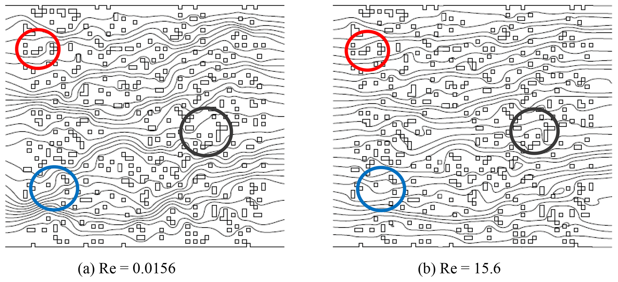
Figure 1Two-dimensional domain containing randomly distributed obstacles (squares and rectangles). Stream functions for (a) Re=0.0156 and (b) Re=15.6 are shown with constant increments between consecutive streamlines (from Andrade et al., 1999; copyright American Physical Society). The different patterns of preferential pathways are clear and distinct. The three pairs of circles (red, blue, black) highlight three (of many) specific locations where the streamlines are seen to change as a function of Re.
Figure 1 demonstrates that the streamlines in individual pores change because of the interplay between inertial and viscous forces given by Re. In other words, with a change in overall fluid velocity or hydraulic gradient across the domain, the actual flow paths can be altered, together with a change in overall and (spatially) local residence times of fluid molecules; the same factors also govern chemical species, as addressed below. Of course, the significantly lower porosities and more tortuous pore space configuration in natural, heterogeneous geological porous media may affect the impact of inertial effects, especially at the pore scale, but the principle remains relevant. We note, too, parenthetically, that the behavior shown in Fig. 1 is also relevant to fluid flow within fracture planes, wherein the obstacles represent contact areas and regions of variable aperture.
Clearly, then, except in highly idealized and simplified geometries, use of a purely analytical solution to identify the full velocity field and streamline patterns at the pore scale is not feasible. Moreover, the extent and changes in streamlines are not intuitively obvious without full numerical solution of the governing flow equations, for any specific set of porous-medium structures and boundary conditions.
2.2 Continuum-scale flow field analysis
Considering now continuum-scale domains, but in analogy to the example shown in Sect. 2.1, we illustrate why knowledge only of the geometrical “static” structure is insufficient to know the flow dynamics, without solution of the Darcy equation. Here, the geometrical structure refers to the spatial distribution of the hydraulic conductivity, K.
Figure 2 represents a realization of a numerically generated (statistically homogeneous, isotropic, Gaussian) hydraulic conductivity 2D domain. The Darcy equation solution for this domain yields values of hydraulic head throughout the domain; these are converted to local velocities to enable delineation of the streamlines and preferential flow paths. The latter are highlighted by actually solving for chemical transport by following the migration of “particles” representative of masses of dissolved chemical species injected along the inlet boundary of the flow domain; see Edery et al. (2014) for details. Of particular significance is that 99.9 % of the injected particles travel in preferential pathways through a limited number of domain cells. We return to Fig. 2 in Sect. 3.3.2, where we discuss a framework that effectively characterizes and quantifies chemical transport.
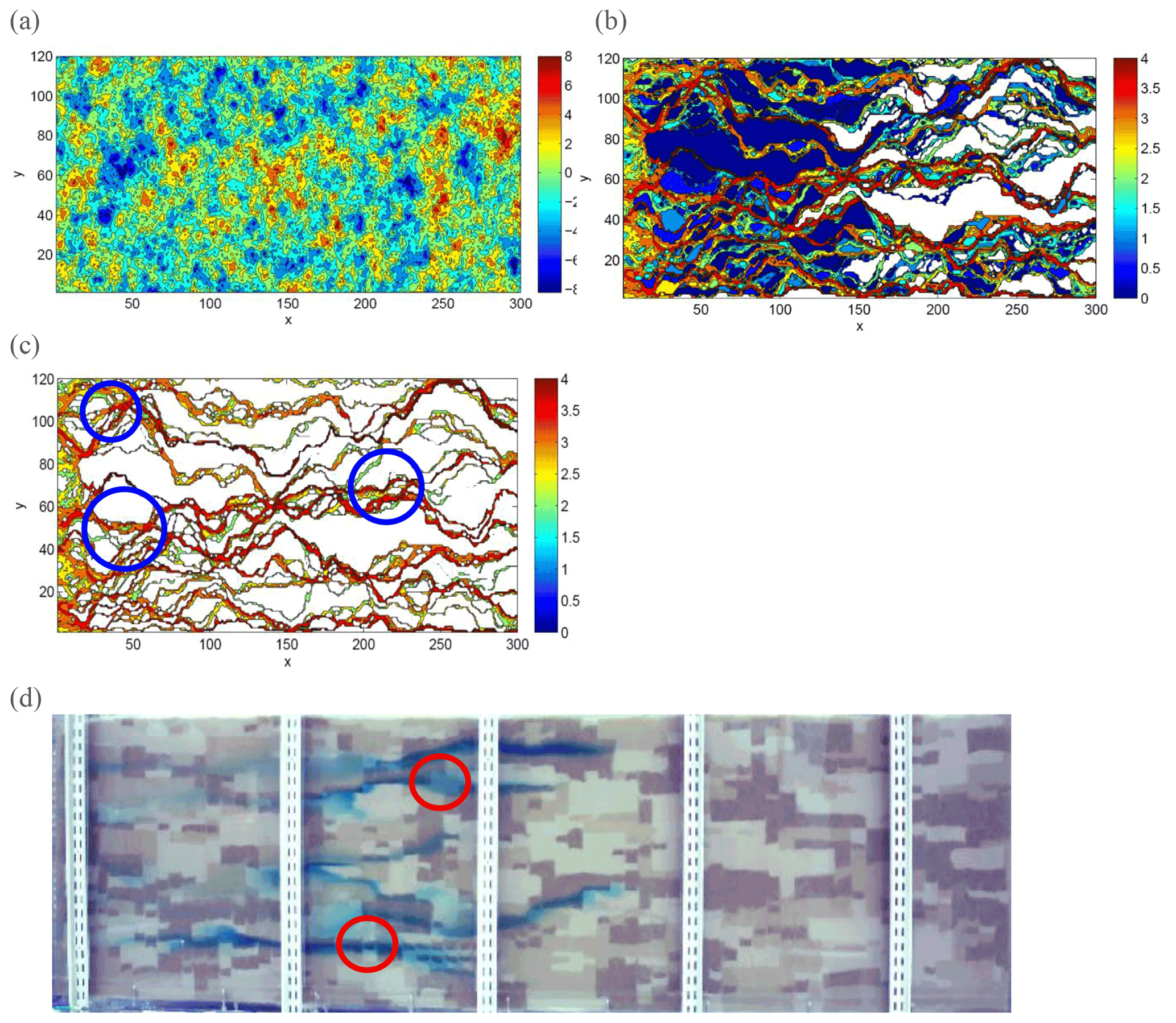
Figure 2Maps of (a) hydraulic conductivity, K, distribution in a domain with 300×120 cells, (b) preferential pathways for fluid flow (and chemical transport), and (c) preferential pathways through cells that each contain a visitation of at least 0.1 % of the total number of chemical species particles injected into the domain (flux-weighted, along the entire inlet boundary). Flow is from left to right. Note that the color bars are in ln (K) scale for (a) and log 10 number of particles for (b, c) (Edery et al., 2014; © with permission from the American Geophysical Union 2014). (d) Laboratory flow cell (dimensions 2.13 (length) × 0.65 (height) × 0.10 (width) m) with an exponentially correlated K structure, showing preferential pathways for blue dye injected near the inlet (flow is left to right); dark-, medium-, and light-colored sands represent high, medium, and low conductivity, respectively (Levy and Berkowitz, 2003; © with permission from Elsevier 2003). The circles shown in (c) and (d) highlight two (of many) regions in which the pathways are seen to contain lower K “bottlenecks”.
Unlike the pore-scale case shown in Sect. 2.1, at the Darcy/continuum scale, streamlines are not altered with changes in the overall hydraulic gradient as long as laminar flow conditions are maintained. And yet, preferential flow paths are (possibly surprisingly) sparse and ramified, sampling only limited regions of a given heterogeneous domain, with the vast fraction of a migrating chemical species that interrogates the domain being even more limited. Significantly, except in highly idealized and simplified geometries, delineation of these pathways is not intuitively obvious (e.g., by simple inspection of the hydraulic conductivity map in Fig. 2a) or definable from a priori analysis or tractable analytical solution. Rather, numerical solution of the governing flow equations is required for any particular/specific set of porous-medium structures and boundary conditions. Note, too, that critical path analysis from percolation theory (discussed in Sect. 2) – again from purely “static” information without solution of the flow field – yields an incorrect interpretation, as shown in detail by Edery et al. (2014).
We emphasize that the delineation of “preferential flow paths” is usually relevant only for study of chemical transport; if water quantity, alone, is the focus, then specific “flow paths” traveled by water molecules – and their advective and diffusive migration along and between streamlines and into/out of less mobile regions – are of little practical interest. On the other hand, the movement of chemical species, which experience similar advective and diffusive transfers, must be monitored closely to be able to quantify overall migration through a domain. We return to considering patterns of chemical migration in Sect. 3. This argument, too, reinforces the assertion that delineation of actual chemical transport cannot be deduced purely from spatial information and solution for fluid flow but must be treated by solution of a transport equation.
It is significant, too, that fluid flow and chemical transport occur in preferential pathways that contain low-conductivity sections (indicated by circles in Fig. 2c and d). How do we explain passage through low-hydraulic-conductivity “bottlenecks” within the preferential pathways rather than migration “only” through the highest-conductivity patches?
To address this question, we first consider what happens in a 1D path. Consider two paths, each containing a series of five porous-medium elements or blocks, with distinct hydraulic conductivity values, Ki. Consider Path 1, with a series of hydraulic conductivity values of 3, 3, 3, 3, and 3, and Path 2, with values 6, 6, 1, 6, and 6 (specific length/time units are irrelevant here). The value of K=1 represents a clear “bottleneck” in an otherwise higher-K path than that of Path 1. In a 1D series, however, the overall hydraulic conductivity (Koverall) of the path is given by the harmonic mean of the conductivities of the elements comprising the path: . Significantly, in the two cases here, both paths have Koverall=3. So, a “bottleneck” (K=1) can be “overcome” and does not cause necessarily a potential pathway to be less “desirable” than a pathway without such “bottlenecks”. In other words, flow through pathways containing some low-K regions should be expected. Of course, in 2D and 3D systems, patterns of heterogeneity and pathway “selection” by water/chemicals are significantly more complicated, but the principle discussed here for 1D systems still holds in the sense that lower-hydraulic-conductivity (“bottleneck”) elements can (and do) exist in the preferential pathways (e.g., Margolin et al., 1998; Bianchi et al., 2011).
We now consider the next level of the “information hierarchy” outlined in Sect. 1.3. To quantify the evolution of a migrating chemical plume, knowledge of the flow field is not generally sufficient, and additional means to characterize and quantify the behavior are needed. Dynamic aspects of chemical transport require us to think (also) in terms of time, not just space and physical structure. Moreover, it is generally insufficient to determine the transport of the chemical plume center of mass. Rather, in terms of water resource contamination and remediation, for example, it is critical to characterize, respectively, the early and late arrival times in compliance or monitoring regions downstream of the point, areal, or volumetric regions in which the chemical species entered the system.
As we show below, it becomes clear that there are dynamic aspects of chemical transport, over and above the role of the flow field: we must actually solve for chemical transport, at either the pore scale or continuum scale, to determine the spatial plume and/or temporal breakthrough curve evolution of the migrating chemical plume. In both the pore-scale and continuum-scale domains, the critical control that arises is that of time, in addition to space. This is in sharp contrast to fluid flow at the pore and continuum scales, as shown in Sect. 2.1 and 2.2: pore-scale fluid flow displays changing streamlines with changes in hydraulic gradient, while continuum-scale fluid flow follows distinct but difficult-to-identify preferential flow paths essentially independent of the hydraulic gradient.
We point out, too, that for both pore-scale and continuum-level scenarios, one can solve explicitly a governing equation for transport. Alternatively, one can obtain an “equivalent” solution by solving for “particle tracking” of transport along the calculated streamlines, in a Lagrangian framework. In other words, particle tracking methods essentially represent an alternative means of solving an (integro-)partial differential equation for chemical transport; such methods can be applied, too, when the precise partial differential equation is unknown or the subject of debate. We also note that solution of the relevant equations for fluid flow and chemical transport is sometimes achieved by (semi-)analytical methods if the flow/transport system can be treated sufficiently simply (e.g., as macroscopically, section-averaged 1D flow and transport in a rectangular domain).
We first discuss principal features of pore-scale (Sect. 3.1) and continuum-scale (Sect. 3.2) chemical transport, and in Sect. 3.3, we focus on effective model formulations. We focus on conservative chemical species and mention chemical reaction effects only peripherally. Note that other factors such as temporally/spatially changing fluid viscosity and surface tension, or mechanical and wetting properties of the solid phase, represent further complexities that are not considered here.
3.1 Pore-scale chemical transport analysis
To illustrate why knowledge only of the flow field is insufficient for full quantification of chemical transport, consider the three porous-medium domains shown in Fig. 3. Each domain is comprised of pore-scale images of a natural rock, modified by enlarging the solid-phase grains, to yield three different configurations: a statistically homogeneous system domain, a weakly correlated system, and a structured, strongly correlated system (see Nissan and Berkowitz, 2019, for details). Fluid flow was determined by solution of the Navier–Stokes equations (Fig. 1a). Transport of a conservative chemical species was then simulated via a (Lagrangian) streamline particle tracking method for an ensemble of particles that advance according to a Langevin equation. Transport behavior was determined for two values of the macroscopic (domain-average) Péclet number (Pe). Recall that , where v is fluid velocity, L is a characteristic linear dimension, and D is the coefficient of molecular diffusion. Here, the macroscopic Pe is based on the mean particle velocity and mean particle displacement distance per transition (or “step”).
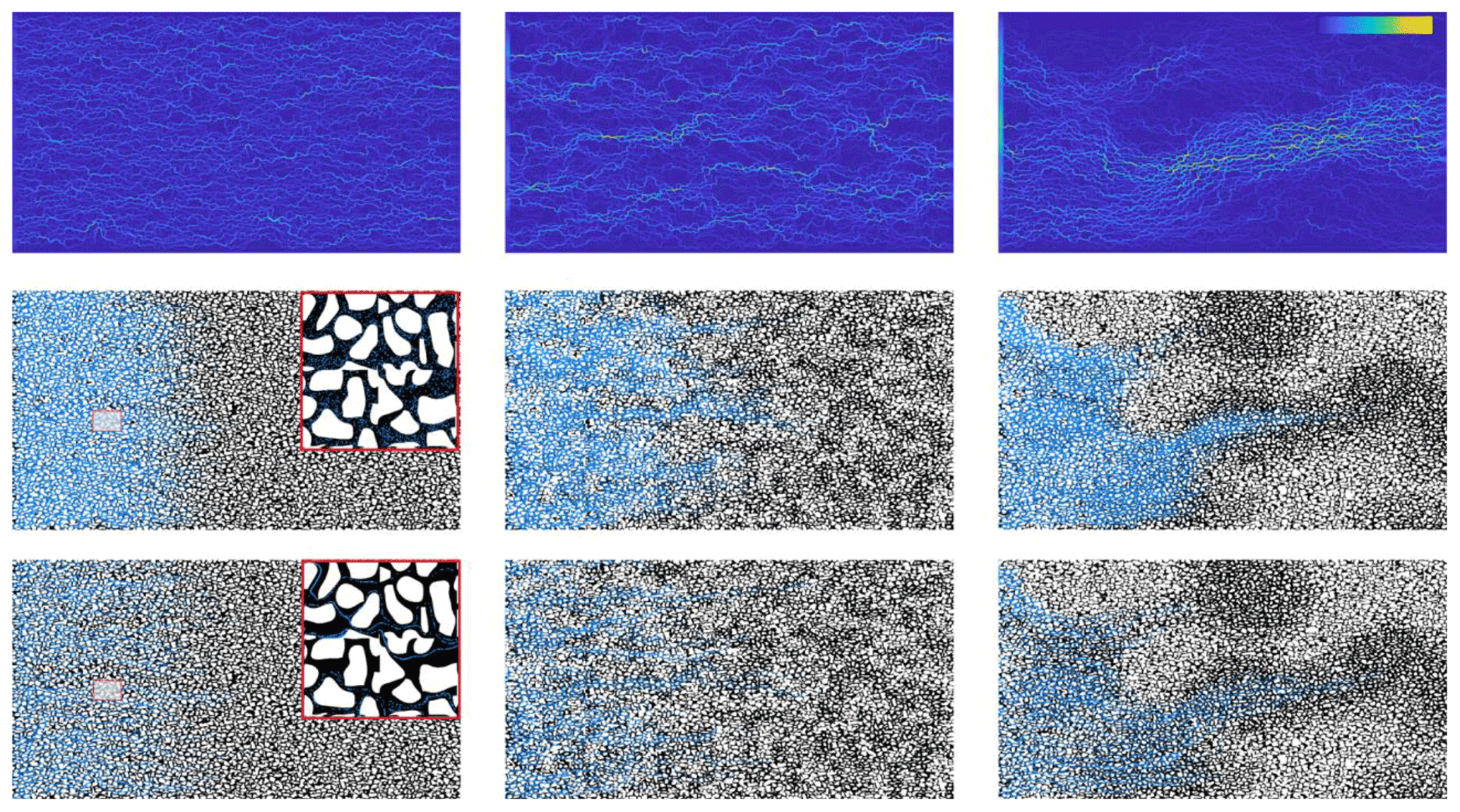
Figure 3Fluid velocities and chemical migration in three porous media configurations (from left to right): homogeneous system, randomly heterogeneous system, and structured heterogeneous system. The upper row shows the (normalized) velocity field for the three configurations; the color bar represents relative velocity, with dark blue being lowest. The middle and lower rows show, respectively, numerically simulated particle tracking patterns of an inert chemical species (blue dots) at Pe=1 (middle row) and Pe=100 (lower row) for the three configurations (white color indicates solid phase; black color indicates liquid phase). Each system has overall dimensions of 8 cm (length) × 6 cm (height). Note: the particle plumes are shown at 10 % of the final time of each simulation; absolute travel times differ among the plots. The insets in the left-hand-side plots of the middle and lower rows show the pore-scale chemical species distributions; note the more diffuse pattern for Pe=1 (from Nissan and Berkowitz, 2019; © with permission from the American Physical Society 2019).
Figure 3 shows that, regardless of possible pore-scale streamline changes as a function of hydraulic gradient (recall Sect. 2.1, considering different values of Re), the choice of macroscopic Péclet number in a given domain plays a significant role in the evolution of the migrating chemical plume. In particular, the relative effects of advection and diffusion, which vary locally in space, are critical, as is the overall residence time in the domain. We stress here, and return to this key point in the discussion below, that the spatially and in some cases temporally local changes in relative effects of advection and diffusion – characterized by the local Pe – dominate determination of the plume evolution. This can be understood from study of Fig. 3 for two choices of macroscopic Pe values in each of the three heterogeneity configurations; the different patterns of longitudinal and transverse spreading are observed clearly.
The behavior shown in Fig. 3 is essentially well known from extensive simulations and experiments appearing in the literature. This behavior is described here to stress the importance of temporal effects and to point out that information only of the advective velocity field – as discussed in Sect. 2.1 and 2.2 – is not sufficient to “predict” chemical transport.
3.2 Continuum-scale chemical transport analysis
The aspects discussed in Sect. 3.1 are relevant, analogous, and applicable essentially also to chemical transport at the continuum scale. Consider the two laboratory experiments shown in Figs. 4 and 5. Each flow cell was filled with a different clean, sieved sand configuration; see Levy and Berkowitz (2003) for details. Figure 4 shows a uniform (“homogeneous”) packing of clean sand, while Fig. 5 shows a coarse sand containing a randomly heterogeneous arrangement of rectangular inclusions consisting of a fine sand. The flow cells, fully saturated with water, enabled macroscopically (section-averaged) 1D, steady-state flow, with a mean gradient parallel to the horizontal axis of the cell. As seen in the two figures, neutrally buoyant, inert red dye was injected at seven (Fig. 4) and five (Fig. 5) points near the inlet side to illustrate the spatiotemporal evolution of the chemical plumes.
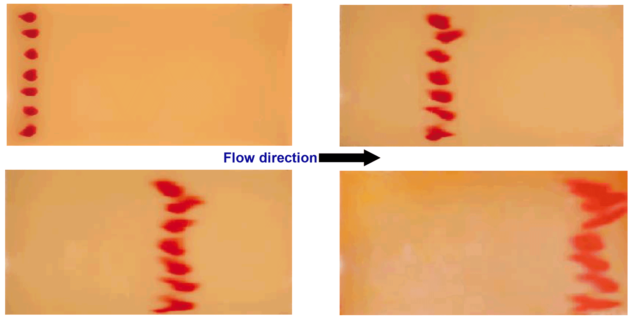
Figure 4Photographs of dye transport in a flow cell (dimensions 0.86 (length) × 0.45 (height) × 0.10 (width) m) containing a uniform packing of quartz sand (average grain diameter 0.532 mm), under a constant flow rate with Pe>1, at four times (Levy and Berkowitz, 2003; © with permission from Elsevier 2003).
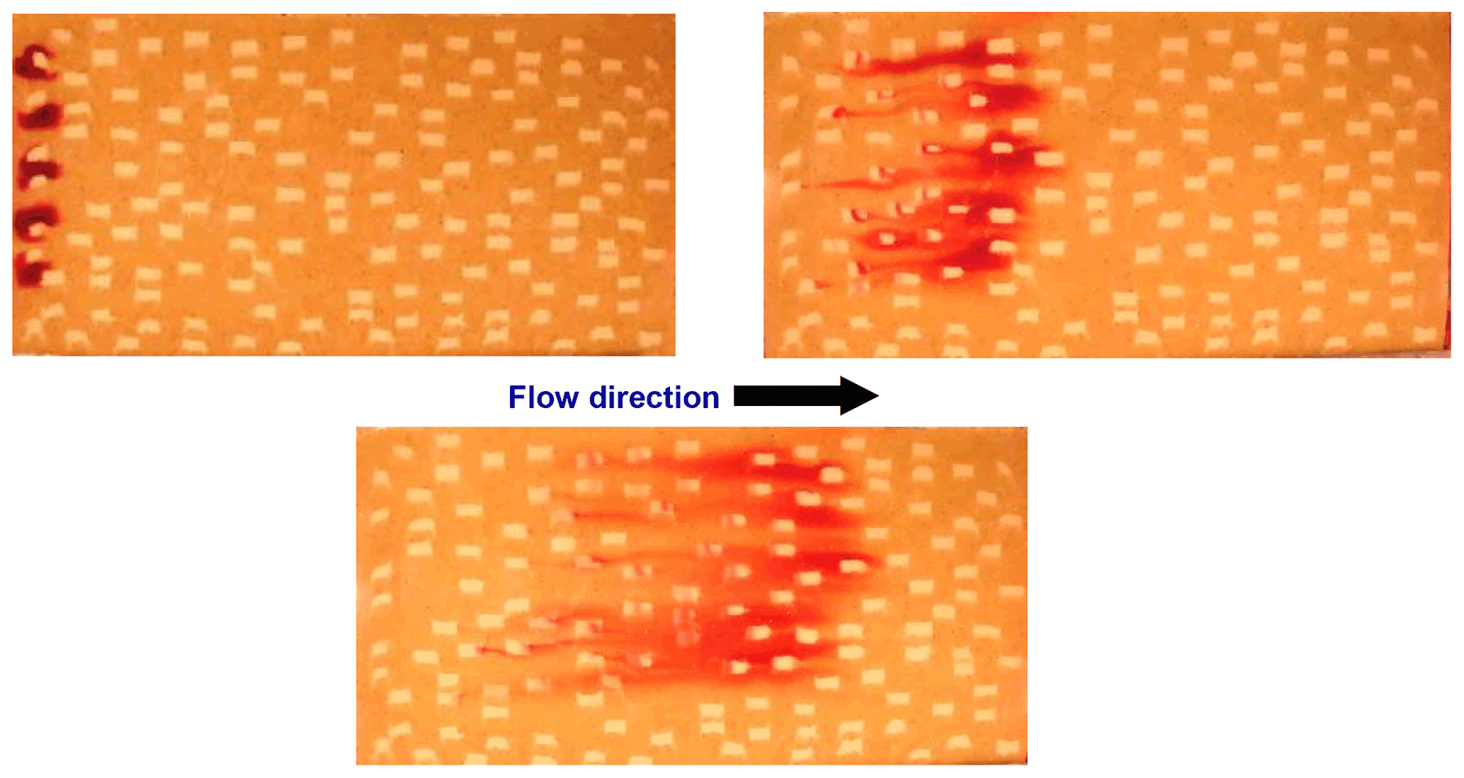
Figure 5Photographs of dye transport in a flow cell (dimensions 0.86 (length) × 0.45 (height) × 0.10 (width) m) containing a randomly heterogeneous packing of quartz sand, under a constant flow rate with Pe>1, at three times. The rectangular inclusions comprise sand with an average grain diameter smaller and hydraulic conductivity lower than the surrounding sand matrix (Levy and Berkowitz, 2003; © with permission from Elsevier 2003).
Most notably, in both Figs. 4 and 5, (i) each of the plumes has a different, unique pattern, which continues over the duration of the plume migration, and (ii) none of the plumes is “elliptical”, as expected in classical Fickian transport theory and embodied in solutions of the classical advection–dispersion equation (ADE). Indeed, vertical averaging of each plume shown in Figs. 4 and 5, at each time, does not yield Gaussian (normally distributed) concentration profiles but rather asymmetrical, “heavy-tailed” profiles.
At this juncture, note that here and below we use the terms “non-Fickian” or “anomalous” – others sometimes use the terms “pre-asymptotic” or “pre-ergodic” – to denote any chemical transport behavior that differs from that described by the classical ADE or a similar type of continuum-scale formulation. Typically, though, non-Fickian transport is characterized by early and/or late arrival times of migrating chemical species to some control or measurement plane/point, relative to those resulting from solution of the ADE. The ADE applies to so-called Fickian behavior, in the sense that it accounts for mechanical dispersion as a macroscopic form of Fick's law; mechanical dispersion arises as an “effective” (or “average”) quantity that describes local fluctuations around the average (advective) fluid velocity. Thus, in this formulation, a pulse of chemical introduced into a macroscopically 1D, uniform velocity, for example, leads to temporal and spatial concentration distributions that are equivalent to a normal (Gaussian) distribution.
It is in this context that the term “homogeneous” packing used above is placed in quotation marks to indicate that in natural geological media, “homogeneity” does not really exist. Any natural geological sample of porous medium contains multiple scales of heterogeneity, and at each particular scale of measurement, “unresolved” heterogeneities that are essentially unmeasurable are present. And thus, as seen in Fig. 4, for example, the overall transport pattern even in a “homogeneous” system can be non-Fickian (anomalous). We therefore emphasize that because natural heterogeneity in geological formations occurs over a broad range of scales, “normal” (Fickian) transport tends to be the “anomaly”, whereas “anomalous” (non-Fickian) transport is ubiquitous and should be considered “normal”.
Moreover, as noted in Sect. 2.2, streamlines are not altered with changes in the overall hydraulic gradient, at the continuum (Darcy) scale, as long as laminar flow conditions are maintained, because increasing the hydraulic gradient increases the fluid velocity along the existing, “pre-defined” streamlines by the same factor. However, the character of chemical transport can be altered, as the change in residence time in the domain affects the relative effects of advection and diffusion space. And in domains with heterogeneous distributions of hydraulic conductivity, the local Pe (Sect. 3.1) can vary more strongly, too.
Thus, we argue that patterns of chemical transport cannot be fully determined from information only on the velocity field; solution of an appropriate continuum-scale transport equation cannot be avoided. In conclusion, then, and with particular reference to the (conceptually and theoretically beautiful) classical ADE – and to “conventional” conceptual understanding and quantitative description of chemical transport – we suggest that one must separate mathematical convenience and wishful thinking from the reality of experiments: there is a definitive need for more powerful formulations of transport equations. In this context, one is reminded of the quotation by the biologist Thomas Henry Huxley: “The great tragedy of science – the slaying of a beautiful theory by an ugly fact.” (President's Address to the British Association for the Advancement of Science, Liverpool Meeting, 14 September 1870)
3.3 Modeling chemical transport and the myth that “fewer parameters are always better”
So how do we effectively model chemical transport?
As noted at the outset of Sect. 2, solution of the Navier–Stokes or Darcy equations to determine the full flow field and velocity distribution in a given porous-medium domain has been proven correct and effective in most applications and is well accepted in the literature. However, modeling of chemical transport is more contentious, the reasons for which we expand upon below.
We argue here that modeling of chemical species transport requires us to think in terms of time, not just space. To assist the reader in entering this frame of thinking and to sharpen our conceptualization, we provide two examples to illustrate aspects of time and space in the context of chemical transport dynamics.
-
The classical example of the brachistochrone (ancient Greek: “shortest time”), or path of fastest descent, is the curve that would carry an idealized point-like body, starting at rest and moving along the curve, without friction, under constant gravity, to a given end point in the shortest time. Somewhat non-intuitively, the path that leads to the shortest travel time is not a straight line, but, rather, a special curve that is longer than a straight line (a cycloid), as demonstrated by Johann Bernoulli in 1697 (see http://old.nationalcurvebank.org//brach/brach.htm, last access: 25 April 2022).
-
What error can be introduced when “averaging” in terms of space? Consider the case of driving a total distance of 100 km, by first traveling 50 km at 1 km h−1 and then traveling 50 km at 99 km h−1. If we average the speed in terms of space (distance), then we traveled two segments of 50 km at two speeds, so the average speed is km h−1. In this framework, the total time to travel the 100 km “should” only have been 2 h. However, in terms of time, the travel time is actually 50.5 h.
These simple examples help to emphasize the errors introduced by traditional conceptual thinking, wherein the effects of spatial transport and domain heterogeneity are quantified only on the basis of spatial characteristics. It is worth recalling, too, Einstein's quantitative treatment of Brownian motion (Einstein, 1905). Prior to his analysis, researchers applied – with puzzlement – a time-dependent velocity, v, to quantify experimental measurements. Einstein (1905) instead examined a recursion relation and expansion that led to a diffusion equation whose solution showed, for the first time, that the root mean squared displacement of particles undergoing Brownian motion is proportional to and not to vt, as had been assumed traditionally. An astounding conceptual breakthrough over a century ago, this nature of diffusive motion is now “common knowledge”.
In this same framework of focusing on time, the examples shown in Figs. 4 and 5 emphasize that, for chemical transport, we must recognize the critical role of rare events. These rare events involve chemical species – migrating “particles” or “packets” – that are held up or retained while traveling through or into/out of lower-velocity regions in the porous domain over various periods of time. Such events can have a dominant impact on overall transport patterns at both the pore and continuum scales. In this context, one must exercise caution with simple averaging of “small-velocity fluctuations” and effects of molecular diffusion. Rather, small-scale heterogeneities in both space and time do not necessarily “average out” or become insignificant at larger scales; rather, the effects of “rare events” (e.g., temporary trapping of even small amounts of chemical species via diffusion into and out of low-velocity regions) and fluctuations can propagate and become magnified, within and across length scales from pore to aquifer.
Armed with these thoughts, we suggest that modeling chemical transport has been debated in the literature for at least three reasons.
-
The desire to work with spatial averaging approaches and equations: the research community was (and still is) split over the need to recognize and incorporate, explicitly, influences of temporal mechanisms caused largely by spatial heterogeneity (as characterized by the domain hydraulic conductivity) when formulating “effective” (or “averaged”) equations. And even when recognized, debate remains as to the appropriate mathematical formulation.
-
The lack of data: at least part of the difficulty in developing appropriate models is the lack of availability of high-resolution laboratory data and field measurements against which chemical transport models can be tested. Indeed, many elaborate theoretical developments have been advanced over the decades, with accompanying analytical and numerical solutions – and yet, remarkably, comparative studies against actual laboratory data remain limited, and tests with field measurements are even sparser (see also Sect. 4 for further discussion of this point).
-
The choice of approach to, and purpose of, chemical transport modeling: two overarching approaches to quantifying chemical transport can be defined, focusing on (i) quantification of “effective”, “overall” chemical transport behavior without requiring high-resolution discretization and numerical solution of the domain, and, alternatively, (ii) high-resolution hydrogeological delineation and then intensive numerical simulation on highly discretized grids. We address approaches (i) and (ii) individually, below, in the context also of points (1) and (2).
The debate in the literature between “effective” and high-resolution hydrogeological modeling, as well as various preconceptions and misconceptions discussed below and in Sect. 4, leads naturally to consideration of the (often incorrectly invoked) argument that “fewer model parameters are better”.
We first discuss briefly aspects of high-resolution hydrogeological modeling in Sect. 3.3.1 and then focus on “effective” transport equation modeling in Sect. 3.3.2. We emphasize that the latter approach is applicable to both small- and large-scale domains. The former approach is generally intended for large- (field-)scale systems, although it is in some sense often applied for detailed pore-scale modeling; this approach is not particularly contentious, per se, but it is hampered by the complexity and cost associated with the demand for highly detailed hydrogeological information. Therefore, research work remains heavily invested in “effective” transport equation modeling.
3.3.1 High-resolution domain delineation and modeling
Efforts to resolve large-scale aquifer systems and to delineate the hydraulic conductivity distribution at increasingly higher resolutions began in earnest in the 1990s. Analysis of field sites emphasized relatively high-resolution discretization of domain structure (e.g., blocks of the order of 10 m3 at the field scale, Eggleston and Rojstaczer, 1998, and m3 at large regional scales, Maples et al., 2019). These efforts, first focusing on determining the fluid flow field and subsequently on delineating pathways for chemical transport, began largely because of dissatisfaction with results of application of 1D, 2D, and 3D forms of an “effective” (averaged) ADE (see further discussion in Sect. 3.3.2). Acquiring high-resolution measurements of structural (e.g., mineralogy, porosity) and hydrological properties (e.g., hydraulic conductivity) was made more feasible in recent years by advances in hydrogeophysics, as well as by advances in computational capabilities that enable incorporation of this information into finely discretized meshes and numerical solution for fluid flow and chemical transport.
In these highly resolved, high-resolution gridded domains, the flow field can be determined from solution of Darcy's law. Chemical transport is then simulated either by use of streamline particle tracking methods, by accounting for advection and diffusion in a Lagrangian framework, or via solution of a local, mesh element continuum-scale transport equation. For chemical transport, use of an advection–diffusion equation might appear preferable – given that it requires no estimate for the local dispersivity – but some researchers apply an advection–dispersion equation, which necessitates use of mesh-scale dispersivity values that are either assumed or estimated from local measurements. The latter case assumes mesh-scale transport to be fully Fickian (recall Sect. 3.2). More recently, alternative formulations of a governing transport equation that incorporates broad temporal effects can also be used in this type of modeling approach; see, e.g., Hansen and Berkowitz (2020) for incorporation of a continuous time random walk method (discussed in Sect. 3.3.2). Parenthetically, we note that “analogous”, high-resolution measurements are made at the pore scale – in millimeter to decimeter rock core samples – as a basis for computationally intensive modeling of fluid flow and chemical transport at these scales. Similarly to the evolution of this approach for field-scale studies, high-resolution measurements advanced from use of 2D rock micrographs to advanced micro-computed tomography protocols (e.g., Thovert and Adler, 2011; Bijeljic et al., 2013; recall Sect. 2.1).
This approach is attractive in terms of the ability to “reproduce” detailed heterogeneous hydraulic conductivity structures and can provide useful “overall assessments” of fluid flow and chemical transport pathways, as well as migration of a chemical plume. Moreover, solutions for fluid flow and chemical transport can be considered “exact”, at least at the scale at which the domain is discretized; they can thus also capture at least some aspects of non-Fickian transport. However, even at this type of spatial resolution, the ability to effectively quantify actual chemical transport, even relative to the limited available field measurements, remains a question of debate; the research community, as well as practicing engineers, still often prefer to analyze chemical transport in a domain by use of relatively simple (often 1D, section-averaged) model formulations.
Finally, we point out that in the context of efforts to obtain increasing amounts of structural and hydrological information at a given field site, due consideration should also be given to the “worth” of data. Thus – for example – in an effort to quantify fluid flow or conservative chemical transport in an aquifer, do we really need “full”, detailed knowledge of the system (e.g. porosity, hydraulic conductivity) at every point in the formation? Possibly non-intuitively, the adage “more data are better” is often not true, and model incorporation of statistical uncertainty can offer equally satisfactory solutions with less costly and less measurement-intensive and computationally intensive detail (e.g., Dai et al., 2016).
3.3.2 “Effective” characterization and modeling
At least since the 1960s, the research community has focused enormous efforts on formulation of “averaged” or “effective” (often macroscopically, section-averaged 1D) transport equations to quantify chemical transport without requiring high-resolution discretization and computationally intensive numerical solution of the domain. The now “classical” ADE was advanced as the governing partial differential equation; see also further discussion on “effective scales of interest” in the context of “upscaling” (Sect. 4). Recall that, as discussed in Sect. 3.2, the ADE assumes Fickian transport behavior, in the sense that mechanical dispersion – which is defined as an average quantity to describe local fluctuations around the average (advective) fluid velocity – is treated macroscopically by Fick's law. The classical ADE then specifies coefficients of longitudinal and transverse dispersivity, which by definition are constants.
Solutions of the ADE were compared against conservative tracer experiments in laboratory columns (generally 10–100 cm) to produce breakthrough curves of concentration vs. time, at a set outlet distance, but even from the outset, the applicability of the ADE was questioned by some researchers (e.g., Aronofsky and Heller, 1957; Scheidegger, 1959). Subsequent flow cell experiments demonstrated, for example, that the dispersivity constants are not actually constant and change with length scale – even over tens of centimeters – to achieve even approximate fits to the measurements (e.g., Silliman and Simpson, 1987). Moreover, solutions of the ADE appear inadequate when compared to transport in laboratory flow cells with distinct regions of different hydraulic conductivities (e.g., Maina et al., 2018). In a sense, then, it can be considered somewhat surprising that this form of the ADE was subsequently assumed to apply, over several decades, in a rather sweeping fashion to a wide range of hydrogeological scenarios and length scales. Detailed discussions of these aspects appear in, e.g., Berkowitz et al. (2006, 2016). Parenthetically, we stress again here that if one has complete information at the pore scale, then solution of the Navier–Stokes and advection–diffusion equations within the pore space can capture the true chemical transport behavior; i.e., purely spatial information is sufficient to describe chemical transport. But, at continuum scales, time and unresolved heterogeneities became critical, and an “averaged” equation like the ADE with a “macrodispersion” concept is problematic.
To move beyond the ADE and the definitive need for effective transport equations that quantify non-Fickian as well as Fickian transport (recall Figs. 4 and 5), we consider an alternative approach. The idea is to account for the temporal distribution that affects chemical migration, in addition to the spatial distribution, at a broad continuum level and employ a transport equation in the spirit of a “general-purpose” ADE. This approach necessarily leads to transport behaviors that are more general than those indicated by a “general ADE”, i.e., in the context of an overall, averaged 1D transport scenario, for example.
To explain this approach, we refer to the continuous time random walk (CTRW) framework, which is particularly broad and general (Berkowitz et al., 2006). Significantly, and conveniently, it turns out that special, or limit, cases of a general CTRW formulation lead to other well-known formulations that can also quantify various types of non-Fickian transport, as explained in, e.g., Dentz and Berkowitz (2003) and Berkowitz et al. (2006). These “subsets” include mobile–immobile (e.g., Feehley et al., 2000), multirate mass transfer (e.g., Haggerty and Gorelick, 1995; Harvey and Gorelick, 1995; Carrera et al., 1998), and time-fractional derivative formulations (e.g., Barkai et al., 2000; Schumer et al., 2003; Metzler and Klafter, 2004). Indeed, in spite of references to these model formulations as being “different”, they are closely related, with clear mathematical correspondence. Each formulation has advantages, depending on the domain, problem, and objectives of model use, but model selection must first be justified physically, and it is inappropriate, for example, to apply a mobile–immobile (two-domain) model to interpret chemical transport in a “uniform, homogeneous” porous medium when it displays non-Fickian transport behavior (recall Fig. 4).
Here, we describe only briefly the principle and basic aspects of the CTRW formulation; detailed explanations and developments are available elsewhere (e.g., Berkowitz et al., 2006).
To introduce “temporal thinking” in the context of non-Fickian transport, we begin by mentioning the analogy between a classical random walk (RW) – which leads to Fick's law – and the CTRW. A classical random walk is given in Eq. (1):
where represents the probability of a random walker (“particle”) advancing from location l′ to l, Pn(l′) denotes the probability of a particle being located at l′ at (fixed) time step n, and Pn+1(l) denotes the probability of the particle then being located at l at step n+1. With this formulation in mind, Einstein (1905) and Smoluchowski (1906a, b) demonstrated that for n sufficiently large and a sufficient number of particles undergoing purely (statistically) random movements in space, the spatial evolution of the particle distribution is equivalent to the solution of the (Fickian) diffusion equation. This elegant discovery demonstrated that a partial differential equation and its solution can be represented by following, numerically, the statistical movement of particles (i.e., particle tracking) following a random walk. Remarkably, random walk formulations are “generic” in the sense that they can be applied in a broad range of phenomena in physics, chemistry, mathematics, and the life sciences; here, they describe naturally migration of chemical species (dissolved “particles” or “packets”) in water-saturated porous media. Generalizing the partial differential equation to include transport by advection, solution of the ADE under various boundary conditions can then be determined by an appropriate random walk method.
The simple random walk given in Eq. (1) can be generalized by accounting for time, replacing the particle transition (or iteration) counter n by a time distribution. The generalized formalism in Eq. (2), with the joint distribution ψ(s,t), called “continuous time random walk” and applied to transport, was first introduced by Scher and Lax (1973):
where is the probability per time of a particle just arriving at site s at time t after n+1 steps and ψ(s,t) is the probability rate for a displacement from location s′ to time s with a difference of arrival times of . It is clear that ψ(s,t) is the generalization of in Eq. (1) and that the particle steps can now each take place at different times. Indeed, it is precisely this explicit accounting of a distribution of temporal contributions to particle transport, not just spatial contributions, that offers the ability to effectively quantify transport behaviors as expressed by, e.g., heavy-tailed, non-Fickian particle arrival times.
Where does the generalization in Eq. (2) lead us? In a mindset similar to that of Brownian motion and Einstein's (1905) breakthrough mentioned above at the outset of Sect. 3.3, a puzzle arose about 7 decades later for researchers attempting to interpret observations of electron transit times in disordered semiconductors. The electron mobility (defined as velocity per unit electric field), which was considered an intrinsic property of the material, was found to depend on variables that changed the duration of the experiment, such as sample length or electric field. Scher and Montroll (1975), considering Eq. (2), discovered that the mean displacement of the electron packet does not advance as but rather as .
In the context of chemical transport in geological formations, the behavior can be attributed to a wide distribution of transition times in naturally disordered geological media. In the CTRW formulation, the transition time distribution is characterized by a power law of the form for t→∞ and ; significantly, the resulting transport behavior is Fickian for β>2. At large times, for this ψ(t) dependence, the mean displacement and standard deviation σ(t) of the migrating chemical plume c(s,t) scale as and σ(t)∼tβ for t→∞, (Shlesinger, 1974). Moreover, for t→∞ with , the plume scales as and . These behaviors are notably different than that of Fickian transport models, for which (from the central limit theorem), and .
With the concepts described here, and using the generally applicable decoupled form , where p(s) is the probability distribution of the transition lengths and ψ(t) is the probability rate for a transition time t between sites, Eq. (2) can be developed into an (integro-)partial differential equation. Thus, the ADE given by
where c(s,t) is the concentration at location s and time t, v(s) is the velocity field, and D(s) is the dispersion tensor, is replaced by the more general CTRW transport equation:
where vψ and Dψ are generalized particle velocity and dispersion, respectively, and M(t) is a temporal memory function based on ψ(t).
The strength of this type of formulation is that it effectively quantifies (non-Fickian) early arrivals and late time tailing of migrating chemical species as well as the spatial evolution of chemical plumes in heterogeneous media. For example, recalling the scenario in Fig. 2, wherein 99.9 % of the inflowing particles traverse the preferential pathways seen in Fig. 2c, detailed numerical simulations indicate that concentration breakthrough curves exhibit significant, non-Fickian, long-time tails (Edery et al., 2014). Choice of an appropriate power-law form of ψ(t) was then shown to capture this behavior; moreover, a functional form defining the value of the power-law exponent β in ψ(t) was identified, based on statistics of the hydraulic conductivity and particle interrogation of the domain (Edery et al., 2014).
Equation (4) is essentially an ADE weighted by a temporal memory. When ψ(t) is an exponential function (or power law but for β≥2), M(t)→δ(t), and we recover Fickian transport described by the ADE; thus, the ADE assumes, implicitly, that particle transition times are distributed exponentially. However, with a power-law form for , the transport is non-Fickian. A wide range of functional forms of ψ(t) can be chosen, including, e.g., truncated power-law forms that allow evolution to Fickian transport at large times or travel distances (e.g., Dentz et al., 2004) as well as Pareto (e.g., Hansen and Berkowitz, 2014) and curved (or inverse gamma; e.g., Nissan and Berkowitz, 2019) temporal distributions. Other, generally simpler, choices of ψ(t) or M(t) lead to mobile–immobile, multirate mass transfer, and time-fractional derivative formulations, as mentioned above. We note, too, that the elegant result derived by Gelhar and Axness (1983) and others, discussed in Sect. 1.2, is valid only at an asymptotic limit, wherein transport is Fickian and there is no residual non-Fickian memory in the plume advance.
A plethora of related studies have examined a range of perspectives and applications that explore CTRW formulations. These studies address, for example, numerical simulations (e.g., Le Borgne et al., 2008; Rhodes et al., 2008; Berkowitz and Scher, 2010; Kang et al., 2014; Nissan and Berkowitz, 2018; Hansen, 2020; Edery, 2021), fractured formations (e.g., Geiger et al., 2010; Wang and Cardenas, 2017), stream transport (e.g., Boano et al., 2007), and laboratory measurements at difference scales (e.g., Le Borgne and Gouze, 2008; Major et al., 2011). Other studies have explored space-fractional differential equations (e.g., Benson et al., 2000; Wang and Barkai, 2020).
Each of these power-law forms of course requires one or more parameters – at least β – and, in some cases, other parameters that define, e.g., a transition time from non-Fickian to Fickian transport (Berkowitz et al., 2006; Hansen and Berkowitz, 2014; Nissan et al., 2017). These parameters have physical meaning and are not purely empirical; perspectives on “numbers of parameters” associated with all models are discussed in Sect. 3.3.3. The question of how model parameter values are determined is addressed in Sect. 4.1.
The efficacy of formulations that incorporate, whether explicitly or implicitly, some type of power-law characterization of temporal aspects of chemical transport is now generally recognized in the literature. Indeed, applications of mobile–immobile, multirate mass transfer, time-fractional advection–dispersion, and general CTRW formulations have been made quite extensively and successfully. In particular, solutions of Eq. (4) and related variants have interpreted a wide range of chemical transport scenarios: (i) pore-scale to meter-scale laboratory experiments, field studies, and numerical simulations, (ii) in porous, fractured, and fractured porous domains, (iii) accounting for constant and time-dependent velocity fields, and (iv) for both conservative and reactive chemical transport scenarios. Solutions to address some of these scenarios are more easily obtained by use of particle tracking methods that incorporate the same considerations and power-law form of ψ(t), as embedded in Eq. (4).
Like the ADE, Eq. (3), the formulation given in Eq. (4) represents a continuum-level mechanistic model (as derived in, e.g., Berkowitz et al., 2002), in the sense that both equations contain clear advective and dispersive contributions. The occurrence of a broad distribution of transition times, fundamental to CTRW and related approaches, emanates from a variety of physical controls. Discussion in the literature about the need for “mechanistic models” often uses the term rather loosely: “mechanistic” transport model equations are based on fundamental laws of physics, with constant parameters that have physical meaning (e.g., hydraulic conductivity, diffusivity, sorption), and thus offer process understanding. However, to quantify the spatiotemporal evolution of a migrating chemical plume, additional parameters are needed. Because of the nature of geological materials, a transport equation should of course capture the relevant physical mechanisms that influence the transport as well as chemical mechanisms if the species is reactive. But to do so, we must also capture the uncertain characterization of hydrogeological properties due to the reality of unresolved, unmeasurable heterogeneities at any length scale of interest. Thus, we suggest that a mechanistic–stochastic equation formulation such as given in Eq. (4) is required. Such an equation (i) incorporates a probability density function to account for temporal transitions that cannot be determined only from spatial information, (ii) describes known transport mechanisms with physically meaningful parameters, and (iii) accounts for unknown (and unknowable) information.
We note here, too, that other stochastic continuum averaging methods have been proposed in the literature in the same context of efforts to formulate a “general”, “effective” transport equation at a specific scale of interest (see further discussion on “effective” equations and “upscaling” in Sect. 4). In many cases, though, sophisticated stochastic averaging and homogenization approaches have led to transport formulations that are essentially intractable, in terms of solution, and/or have remained at the level of hypothesis without being tested successfully against actual data.
3.3.3 Are fewer parameters always better? (Answer: no!)
The term “modeling” is used in many contexts and with differing intents. However, in the literature dealing with chemical transport in subsurface hydrological systems, there are frequent but often misguided “arguments” regarding “which model is better”, with a major point of some authors being the claim that “fewer parameters are always best”. Not always. Indeed, some models involve more parameters than others, but if these parameters have physical meaning and are needed as factors to quantify key mechanisms, then “more parameters” are not a “weakness”. We emphasize, too, that when weighing the use of any specific model, “better” also depends, at least in part, on what the modeling effort is addressing. Clearly – regardless of the number of parameters – a “back-of-the-envelope” calculation using a simple model is sufficient if, for example, one requires only an order of magnitude estimate of the center-of-mass velocity of a migrating contaminant plume or, in other words, no need for artillery to swat a mosquito. In this context, quoting Albert Einstein regarding his simplification of physics into general relativity, “Everything should be made as simple as possible, but not simpler.”
Considering chemical transport in subsurface geological formations and the aim of quantifying (modeling) the evolution of a migrating chemical plume in both space and time, we return to focus on the ADE- and CTRW-based formulations discussed in Sect. 3.3.2. As noted in the preceding sections, CTRW and related formulations can describe transport behaviors effectively. Most significantly, the seminal work of Scher and Montroll (1975) showed that the β exponent must be included because the mean displacement is not linear with time (i.e., the mean displacement of the electron packet does not advance as but rather as ). Similarly, a corresponding parameter, relative to an ADE formulation invoking Fickian transport, is unavoidable when transport is non-Fickian.
It should be recognized that quantitative model information criteria, or model selection criteria, can be used to assess and compare various model formulations that are applied to diverse scenarios (such as fluid flow or chemical transport) in subsurface geological formations. These information criteria (IC) include AIC (Akaike, 1974), AICc (Hurvich and Tsai, 1989), and KIC (Kashyap, 1982) measures as well as the Bayesian (or Schwarz) BIC (Schwarz, 1978). They are formulated to rank models or assign (probabilistic) posterior weights to various models in a multimodel comparative framework and therefore focus on model parameter estimates and the associated estimation uncertainty. As such, these information criteria discriminate among various models according to (i) the ability to reproduce system behavior and (ii) the structural complexity and number of parameters. Discussion of theoretical and applied features of these criteria is given elsewhere (e.g., Ye et al., 2008). Using such measures specifically in the context of the ADE and CTRW formulations, with an accounting also of chemical reactions, it was shown that while solution of an ADE can fit measurements from some locations quite closely, the CTRW formulation offers significantly improved predictive capabilities when examined against an entire experimental data set (Ciriello et al., 2015). In addition, focusing on the most sensitive observations associated with the CTRW model provides a stronger basis for model prediction relative to the most sensitive observations corresponding to the ADE model.
To conclude this section: notwithstanding the above arguments, some readers might continue to argue that the approach discussed here – viz. the need for time considerations as well as space such as embodied in the CTRW framework and related formulations – is “inelegant” because it requires more parameters relative to the classical ADE. In response, the reader is encouraged to recall the words of Albert Einstein following criticism that his theory of gravitation was “far more complex” than Newton's. His response was simple: “If you are out to describe the truth, leave elegance to the tailor”.
We begin by defining the term “upscaling” in the context of the discussion here on chemical transport. As defined in the Introduction, Sect. 1.2, we use the term “upscaling” to describe the effort to develop and apply chemical transport equations at large length scales, and identify corresponding model parameter values, based on measurements and parameter values obtained at significantly smaller length scales.
We attempt “upscaling” in the hope of developing governing equations for chemical transport at larger and larger scales, from pore, to core, to plot, and to field length scales. Clearly, then, “upscaling” is relevant to the modeling approach discussed in Sect. 3.3.2 – which focuses on use of “averaged” or “effective” (often 1D or section-averaged) transport equations – and not to the high-resolution domain delineation and modeling approach of Sect. 3.3.1.
However, in light of the discussion in Sects. 2 and 3, we argue that upscaling of chemical transport equations is very much an unattainable holy grail. Particularly in light of recognizing temporal effects, in addition to spatial characterization, we maintain that it is necessary to formulate and calibrate models, and then apply them, at similar measurement scales of interest. Of course, similar equation formulations can be applied at different spatial scales. However, parameter values for transport equations cannot generally be determined a priori or from purely spatial or flow-only measurements; measurements with a temporal “component”, at the relevant length scale of interest, are required.
In Sect. 4.1, we briefly discuss aspects of model calibration. This leads naturally to our discussion of upscaling in Sect. 4.2.
4.1 Parameter determination and model calibration
First, it is prudent to offer some words about the need for parameter estimation or model calibration. Unless one is dealing with first principles calculations of a physical process such as molecular diffusion in a perfectly homogeneous domain, a priori determination of model parameters – for any model equation formulation – requires calibration against actual experimental measurements. In some limited cases, detailed numerical simulations can be used at small (pore) scales, e.g., using an advection–diffusion equation together with solution of the Navier–Stokes equations to first determine the precise flow field in the pore space, but this also necessitates detailed measurements of the pore structure such as obtained by computed tomography measurements (e.g., Bijeljic et al., 2013). Indeed, then, at any realistic problem or scale of interest, all chemical transport models require calibration.
This fundamental tenet should be clear and well recognized, yet the literature contains all-too-frequent – and both misguided and misleading – “criticism” of various model formulations, claiming that “parameters are empirical because they are estimated by calibration (fitting) to experiments”; additional “criticisms” follow, for example, that such a model is therefore not “universal” and/or that “it therefore has no predictive capability”. We address these latter “criticisms” in Sect. 4.2. Parameters are not “empirical” simply because their values are determined by matching to an experiment. Moreover, it should be recognized that application even of the classical ADE at various column and larger scales requires estimates – obtained by calibration – of dispersivity coefficients; and for high-resolution domain delineation and modeling as discussed in Sect. 3.3.1, calibrated “block-scale” dispersivities are needed. Note that if dispersivities are not actually determined for a specific experiment but selected from the literature for “typical” values of dispersivity, there is still a reliance on calibration from previous “similar” studies. Moreover, with reference to the desire for model parameters that represent fundamental, spatial hydrogeological properties of the domain, note that even the classical ADE dispersivity parameter is not uniquely identified with such properties; rather, it varies even in a given domain as a function of chemical plume travel distance or time.
With regard to model “universality”, recall that, for example, percolation theory (discussed at the beginning of Sect. 2) offers “universal” exponents in scaling relationships. However, even for this type of convenient and useful, statistical model, such scaling relationships, too, can only advance from “scaling” (e.g., A∼B) to a full “equation” (e.g., A=kB) by calibration of a coefficient of equality (k) against actual measurements. So, even in “simple” models, model calibration cannot be avoided.
To address “empiricism” – here enters the question of whether parameters of a particular model (in this case, equations for chemical transport) have a physical meaning. As discussed in Sect. 3.3.2, a mechanistic–stochastic equation formulation such as given in Eq. (4) incorporates a probability density function to describe known transport mechanisms in a stochastic sense; but stochastic does not mean “unphysical”, and the parameters as given in, e.g., particular functional forms of M(t) or ψ(t) are indeed physically meaningful. For example, the key β-exponent characterizing the power-law behavior can be linked directly to the statistics of the hydraulic conductivity field (Edery et al., 2014) or, in a fracture network, determined from the velocity distribution in fracture segments (Berkowitz and Scher, 1998), which is related directly to physical properties of the domain. Similarly, corresponding parameters appearing in “subset” formulations to quantify non-Fickian transport – e.g., mobile–immobile, multirate mass transfer, and time-fractional derivative formulations – can be understood to have physical meaning (e.g., Haggerty and Gorelick, 1995; Harvey and Gorelick, 1995; Carrera et al., 1998; Dentz and Berkowitz, 2003; Berkowitz et al., 2006). These parameters, too, of course require determination by model calibration to experimental data, or where appropriate to results of numerical simulations, just as for ADE and any other model formulation.
4.2 Upscaling, the scale of interest, and predictive capabilities
Upscaling of fluid flow “works” because at the Darcy scale – which is the “practical” scale for most applications – flow paths and streamlines do not change with increasing gradient as long as a transition to turbulent flow is not reached. The equation formulation remains valid, and the fluid residence time in a domain is irrelevant because self-diffusion of water does not affect overall fluid fluxes.
For chemical transport, though, the situation is totally different. Why? Because “upscaling” entails some kind of “coupled” averaging or parameterization in both space and time, and it is far from clear how, if at all, this can be achieved. Moreover, small-scale concentration fluctuations do not necessarily “average out” but instead propagate from local to larger spatial scales. To illustrate another aspect of the complexity, the Péclet number (Pe) in heterogeneous media, with preferential pathways, varies locally in space (recall Fig. 3 and the discussion in Sect. 3.1). Averaging to obtain a macroscale (“upscaled”) Pe must address the relative, locally varying effects of advection and diffusion in space as well as the overall residence time in the domain; after all, it is these effects that dominate determination of the plume evolution. Thus, upscaling requires spatial averaging, but (at least an) implicit temporal averaging must also be included. It can be argued that no single, effective Pe can be defined for the entire domain; whether or not it is possible, and how it is possible to average local Pe values to achieve a single, meaningful domain-scale Pe remains an open question. And whether we like it or not, even with complete information on the spatial (local) Pe distribution, the impact on the overall transport pattern evolution cannot be determined without actually solving for transport in the domain.
For chemically reactive species, the transport situation becomes even more complex, because the local residence time, not just the local Pe, must be taken into consideration. Moreover, when precipitation or dissolution processes are present, the velocity field will change locally, introducing additional local temporal and spatial variability. And when sorption is present but tapers off – for example, when the cation exchange capacity is met – even the diffusion coefficient itself changes. These factors further complicate attempts to upscale. In this context, too, it should be noted that for chemically reactive systems, it is well known that there is often a significant lack of correspondence between laboratory and field-based estimates of geochemical reaction rates and rates of rock weathering, with field-scale estimates – often based on macroscopically Fickian, ADE-like transport formulations – being generally significantly smaller (e.g., White and Brantley, 2003).
Thus, we suggest that focusing efforts on attempting to develop upscaling methodologies for chemical transport, based on any transport equation formulation, appears to be doomed largely to failure – as evidenced, too, by decades of research publications. Rather, we argue that because of the subtle effects of temporal mechanisms and their close coupling to spatial mechanisms, use of an “effective” or “averaged” continuum-level equation to describe chemical transport requires calibration of a suitable model at the appropriate scale of interest, with model parameter values calibrated at essentially the same scale. The model can then be applied to examine transport behaviors over spatial scales with relatively similar orders of magnitude.
We emphasize, though, that as stated at the outset in Sect. 4, we do argue that similar (continuum-level) transport equation formulations can be applied at different spatial scales, as long as they are mechanistically correct, with a temporal component, and the parameter values are based on measurements at the relevant length scale of interest.
Now, in the context of the above arguments regarding “upscaling” and model application, we return to the ideas presented in Sect. 3.3.2 and consideration of model formulations that account for both spatial and temporal effects. We first mention use of the ADE. As pointed out in Sect. 3.2 and the extensive literature, the “constant” (as required by the ADE formulation) “intrinsic” dispersivity parameter changes significantly even over relatively small increases in length scales (e.g., tens of centimeters; Silliman and Simpson, 1987) – and therefore also over timescales. It therefore makes no real sense to attempt to define an “upscaled” dispersivity parameter for larger scales. Even in the framework of high-resolution domain delineation and modeling, discussed in Sect. 3.3.1 – which is not “upscaling” as defined here – the question remains as to which dispersivity values are relevant for field-scale aquifer “blocks” of the order of 100s to 1000s of cubic meters.
In contrast, CTRW and related transport formulations with explicit accounting of time effects, as outlined in Sect. 3.3.2, can be applied meaningfully to interpret real measurements and transport behavior at “all” scales. We can use the same equation formulation at different scales, with different but relevant parameters at each scale. We emphasize, too, that we do not argue for “hard” length scales: in principle, e.g., an appropriate CTRW-based model calibrated at 20 cm will be applicable to 100 cm scales, and a model calibrated on a 100 m scale data set can be applicable at a kilometer scale (e.g., Berkowitz and Scher, 1998, 2009; Rhodes et al., 2008; Geiger et al., 2010; Edery, 2021). The point, though, is that it makes no sense to calibrate at a centimeter scale and then expect to somehow “upscale” parameters to apply the same model at a kilometer scale. Note that, as an aside, over very large field-length and field-time scales, we point out that homogenization effects of molecular diffusion may become more significant, lessening impacts of some preferential pathways. Similarly, a CTRW-based approach can be applied over a range of timescales, because the power law accounting for temporal effects can be as broad as needed. In these cases, temporal effects are critical, because at the continuum (Darcy) scale, streamlines do not change but residence times do. Specifically, for example, a model formulation with a fixed set of parameters can interpret transport measurements in the same domain, but acquired under different hydraulic gradients or fluid velocities, and thus domain residence times (Berkowitz and Scher, 2009). Indeed, because of the temporal accounting, CTRW has been applied successfully over scales from pores (e.g., Bijeljic et al., 2013) to kilometers (e.g., Goeppert et al., 2020), with parameter calibration at the relevant scale of interest. In principle, then, a calibrated model shown to be meaningful over one region of a porous medium or geological formation can offer at least a reasonable estimate of transport behavior elsewhere in the medium/formation, at a similar length scale/timescale, and as long as the medium/formation can be expected to have reasonably similar hydrogeological structure and properties.
Finally, another critical aspect must be pointed out with regard to continuum-scale transport models as outlined in Sect. 3.2. The preceding discussion leads to the stated need and desire – at least in principle – to achieve model “prediction”. This term appears often, but it is often used incorrectly. Fitting a model solution to data is of course not “prediction”. On the one hand, using specific experiments and data sets, models can be used to characterize transport behavior, e.g., whether transport is Fickian or non-Fickian, or whether a migrating chemical plume is compact or elongated and ramified, which is of fundamental importance. However, if prediction is the ultimate goal (recognizing that addressing prediction uncertainty is yet another consideration), then we require multiple data sets from the same porous medium or geological formation, in the sense that we need measurements over a range of length scales and/or over a range of timescales (i.e., same distance, different flow rates). An intended model can then be calibrated against one part of the data set; the calibrated model is then applied “as is”, and the resulting solution, a “prediction”, is compared against other “previously unknown” measurements. At the laboratory scale, such a protocol is feasible but rarely executed. Rather, the literature generally reports fits of transport equation solutions at specific scales – individual data sets at a given length scale – and not over a range of scales, so that no real testing of “upscaling” or “prediction” is achieved. Thus, even at laboratory scales, the true “predictive capability” of a model is rarely examined or reported. Note that a similar approach to “prediction” can be done in a purely numerical/computational study, using “ground truth simulations” that are assumed to be correct (e.g., Darcy flow calculations and then streamline particle tracking for chemical transport in a highly resolved domain; recall Sect. 3.3.1) and then comparing solutions from a continuum (partial differential equation) model solution. However, it should be recognized that results from assumed simulation methods are often unsatisfactory when compared against experimental measurements and field observations.
At the field scale, the situation is even less satisfactory: large-scale field tests for chemical transport are difficult and expensive to execute, so that systematic data sets that enable testing of model “prediction” – as well as even initial calibration of a transport model – are essentially non-existent. Moreover, while larger-scale structural features can be identified in principle via non-invasive geophysical methods, higher-resolution sampling and measurements of hydraulic conductivity and geochemical parameters are necessarily highly limited. As a result, oft-used, non-unique interpolation of sparse concentration measurements is employed to yield (ideally 3D) contour maps of hydrogeological parameters and actual chemical concentrations, but interpolation will unrealistically smoothen and dampen existing ramified and irregular preferential pathways (recall Fig. 2). Thus, notwithstanding the extensive research efforts reported in the literature, truly comparative studies using field measurements – to genuinely test proposed “upscaling” methodologies – are essentially non-existent (e.g., Berkowitz et al., 2016). In this context, then, we note that criticism in the literature that a given continuum model “demonstrates no predictive capability” is in fact not generally based on its assessment relative to sufficiently resolved, representative, and real data sets. Finally, it is important to recognize that models are most commonly tested against 1D, section-averaged concentration breakthrough curves, which can be (i) measured directly in laboratory column experiments, (ii) estimated or derived in 2D/3D laboratory flow cells by averaging over control planes, or (iii) estimated from limited monitoring well measurements (single- or multi-level sampling with depth) at a fixed number of locations. The latter case, in particular, requires extensive interpolation and/or assumption of a large-scale, essentially 1D and uniform macroscopic flow field. Moreover, chemical transport model discrimination often requires breakthrough curves that extend over the late time tailing, which are particularly difficult to determine in field conditions, due both to interruptions or lack of practicality in well monitoring at long times and to detection limits of measurement methods. While reliance on such 1D (section-averaged, over some control plane) breakthrough curves may not be ideal, it is often the reality in terms of feasible data acquisition. As a direct consequence, model selection, model parameter fits, and model calibration results may each (and all) be non-unique and lead to confusing or conflicting conclusions. It is therefore critical that we at least select from mechanistic–stochastic models based on fundamental laws of physics, with parameters that have physical meaning, as discussed in Sect. 3.3.2, rather than from models invoking purely statistical distributions or assumptions known to be incorrect.
The ideas, arguments, and perspectives offered here represent an effort to somehow summarize and synthesize an understanding of existing approaches and methods proposed to quantify conservative chemical transport in subsurface hydrological systems. The literature on this subject is vast, extending over decades, and measurements and observations of chemical transport range from pore-scale microfluidic laboratory cells to aquifer field scales. A similarly broad range of model formulations has been proposed to quantify and interpret these measurements/observations. And yet outcomes of these efforts are often largely unsatisfactory.
We contend that modeling obstacles arise largely because domain heterogeneity – in terms of porosity, hydraulic conductivity, and geochemical properties – is present over multiple length scales, so that “unresolved”, practically unmeasurable heterogeneities and preferential pathways arise at every length scale. Moreover, while spatial averaging approaches are effective when considering overall fluid flow – wherein pressure propagation is essentially instantaneous and the system is “well mixed” – purely spatial averaging approaches are far less effective for chemical transport, essentially because well-mixed conditions do not prevail. We assert here that an explicit accounting of temporal information, under uncertainty, is an additional – but fundamental – component in an effective modeling formulation. As a consequence, we argue that for continuum-scale analysis, mechanistic–stochastic models such as those outlined in Sect. 3.2 must be invoked to account explicitly for both “additional” temporal effects and unresolved heterogeneity. Clearly, no single model is “best” for all situations and objectives, but any selected model must be physically relevant and justified.
We further assert, as an outcome of these arguments, that “upscaling” of chemical transport equations – in the sense of attempting to develop and apply chemical transport equations at large length scales based on measurements and model parameter values obtained at significantly smaller length scales – is very much an unattainable holy grail. Rather, because probabilistic considerations required to account for small-scale fluctuations do not necessarily “average out” – and can propagate from local to larger spatial scales – we maintain that it is necessary to formulate and calibrate models and then apply them over spatial scales with similar orders of magnitude.
In all of our efforts to reasonably model chemical transport in subsurface hydrological systems, we should recognize and accept the objective of advancing our science by integrating theory, computational techniques, laboratory experiments, and field measurement, with the aim of extracting broadly applicable insights and establishing practical, functional tools. In this context, as a close colleague and mentor said to me many, many years ago, “remember, this is hydrology, with very real problems to address … we're not doing string theory”.
We have included many points for discussion and open thought. Understandably, the reader may not agree with all arguments and conclusions raised here, but scholarly debate is critical: it is hoped that this contribution will stimulate further discussion, assist in ordering classification of the (often confusing) terminologies and considerations, and identify the most relevant, real questions for analysis, implementation, and future research.
We hope that the above thoughts and illustrations (i) encourage careful consideration prior to data collection, whether from field measurements, laboratory experiments, and/or numerical simulations, (ii) assist in experimental design and subsequent analysis, and, even more significantly, (iii) influence the research agenda for the field by challenging researchers to ask and address appropriately formulated questions. In terms of “modeling” efforts: recall the statement by Manfred Eigen (Nobel Prize in Chemistry, 1967): “A theory has only the alternative of being right or wrong. A model has a third possibility: it may be right, but irrelevant.”
All data have been reported and published previously, as given in the relevant citations.
The author is a member of the editorial board of Hydrology and Earth System Sciences. The peer-review process was guided by an independent editor, and the author has no other competing interests to declare.
This contribution has emanated from research and discussions – often animated and always thought-provoking – with students, post-doctoral fellows, and more senior colleagues in my group and from around the world, over the last 3 decades. I am deeply grateful to them all. I also appreciate critical insights and constructive comments by Alberto Guadagnini and Harvey Scher. Brian Berkowitz holds the Sam Zuckerberg Professorial Chair in Hydrology.
Publisher's note: Copernicus Publications remains neutral with regard to jurisdictional claims in published maps and institutional affiliations.
This paper was edited by Thom Bogaard and reviewed by John Selker and one anonymous referee.
Akaike, H.: A new look at statistical model identification, IEEE T. Autom. Control, 19, 716–723, https://doi.org/10.1109/TAC.1974.1100705, 1974.
Andrade, J. S., Costa, U. M. S., Almeida, M. P., Makse, H. A., and Stanley, H. E.: Inertial effects on fluid flow through disordered porous media, Phys. Rev. Lett., 82, 5249, https://doi.org/10.1103/PhysRevLett.82.5249, 1999.
Aronofsky, J. S. and Heller, J. P.: A diffusion model to explain mixing of flowing miscible fluids in porous media, T. Am. Inst. Min. Metall. Pet. Eng., 210, 345–349, 1957.
Barkai, E., Metzler, R., and Klafter, J.: From continuous time random walks to the fractional Fokker–Planck equation, Phys. Rev. E, 61, 132–138, https://doi.org/10.1103/PhysRevE.61.132, 2000.
Benson, D. A., Wheatcraft, S. W., and Meerschaert, M. M.: The fractional-order governing equation of Lévy motion, Water Resour. Res., 36, 1413–1423, https://doi.org/10.1029/2000WR900032, 2000.
Berkowitz, B.: Analysis of fracture network connectivity using percolation theory, Math. Geol., 27, 467–483, https://doi.org/10.1007/BF02084422, 1995.
Berkowitz, B. and Scher, H.: Theory of anomalous chemical transport in fracture networks, Phys. Rev. E, 57, 5858–5869, https://doi.org/10.1103/PhysRevE.57.5858, 1998.
Berkowitz, B. and Scher, H.: Exploring the nature of non-Fickian transport in laboratory experiments, Adv. Water Resour., 32, 750–755, https://doi.org/10.1016/j.advwatres.2008.05.004, 2009.
Berkowitz, B. and Scher, H.: Anomalous transport in correlated velocity fields, Phys. Rev. E, 81, 011128, https://doi.org/10.1103/PhysRevE.81.011128, 2010.
Berkowitz, B., Klafter, J., Metzler, R., and Scher, H.: Physical pictures of transport in heterogeneous media: Advection-dispersion, random-walk, and fractional derivative formulations, Water Resour. Res., 38, 1191, https://doi.org/10.1029/2001WR001030, 2002.
Berkowitz, B., Cortis, A., Dentz, M., and Scher, H.: Modeling non-Fickian transport in geological formations as a continuous time random walk, Rev. Geophys., 44, RG2003, https://doi.org/10.1029/2005RG000178, 2006.
Berkowitz, B., Dror, I., Hansen, S. K., and Scher, H.: Measurements and models of reactive transport in geological media, Rev. Geophys., 54, 930–986, https://doi.org/10.1002/2016RG000524, 2016.
Bianchi, M., Zheng, C., Wilson, C., Tick, G. R., Liu, G., and Gorelick, S. M.: Spatial connectivity in a highly heterogeneous aquifer: From cores to preferential flow paths, Water Resour. Res., 47, W05524, https://doi.org/10.1029/2009WR008966, 2011.
Bijeljic, B., Raeini, A., Mostaghimi, P., and Blunt, M. J.: Predictions of non-Fickian solute transport in different classes of porous media using direct simulation on pore-scale images, Phys. Rev. E, 87, 013011, https://doi.org/10.1103/PhysRevE.87.013011, 2013.
Boano, F., Packman, A. I., Cortis, A., Revelli, R., and Ridolfi, L.: A continuous time random walk approach to the stream transport of solutes, Water Resour. Res., 43, W10425, https://doi.org/10.1029/2007WR006062, 2007.
Carrera, J., Sánchez-Vila, X., Benet, I., Medina, A., Galarza, G., and Guimerà, J.: On matrix diffusion: Formulations, solution methods, and qualitative effects, Hydrogeol. J., 6, 178–190, 1998.
Ciriello, V., Edery, Y., Guadagnini, A., and Berkowitz, B.: Multimodel framework for characterization of transport in porous media, Water Resour. Res., 51, 3384–3402, https://doi.org/10.1002/2015WR017047, 2015.
Dagan, G.: Flow and Transport in Porous Formations, Springer, New York, ISBN 13: 978-3-540-51098-7, https://doi.org/10.1007/978-3-642-75015-1, 1989.
Dagan, G. and Neuman, S. P.: Subsurface Flow and Transport: A Stochastic Approach, Cambridge Univ. Press, New York, ISBN 0-521-57257-6, 1997.
Dai, C., Xue, L., Zhang, D., and Guadagnini, A.: Data-worth analysis through probabilistic collocation-based ensemble Kalman filter, J. Hydrol., 540, 488–503, https://doi.org/10.1016/j.jhydrol.2016.06.037, 2016.
Dentz, M. and Berkowitz, B.: Transport behavior of a passive solute in continuous time random walks and multirate mass transfer, Water Resour. Res., 39, 1111, https://doi.org/10.1029/2001WR001163, 2003.
Dentz, M., Cortis, A., Scher, H., and Berkowitz, B.: Time behavior of solute transport in heterogeneous media: Transition from anomalous to normal transport, Adv. Water Resour., 27, 155–173, https://doi.org/10.1016/j.advwatres.2003.11.002, 2004.
Edery, Y.: The effect of varying correlation lengths on anomalous transport, Transp. Porous Med., 137, 345–364, https://doi.org/10.1007/s11242-021-01563-9, 2021.
Edery, Y., Guadagnini, A., Scher, H., and Berkowitz, B.: Origins of anomalous transport in disordered media: Structural and dynamic controls, Water Resour. Res., 50, 1490–1505, https://doi.org/10.1002/2013WR015111, 2014.
Eggleston, J. and Rojstaczer, S.: Identification of large-scale hydraulic conductivity trends and the influence of trends on contaminant transport, Water Resour. Res., 34, 2155–2168, https://doi.org/10.1029/98WR01475, 1998.
Einstein, A.: Über die von der molekulartheoretischen Theorie der Wärme geforderte Bewegung von in ruhenden Flüssigkeiten suspendierten Teilchen, Ann. Phys. Leipzig, 17, 549–560, https://doi.org/10.1002/andp.19053220806, 1905.
Feehley, C. E., Zheng, C., and Molz, F. J.: A dual-domain mass transfer approach for modeling solute transport in heterogeneous aquifers: Application to the macrodispersion experiment (MADE) site, Water Resour. Res., 36, 2501–2515, https://doi.org/10.1029/2000WR900148, 2000.
Geiger, S., Cortis, A., and Birkholzer, J. T.: Upscaling solute transport in naturally fractured porous media with the continuous time random walk method, Water Resour. Res., 46, W12530, https://doi.org/10.1029/2010WR009133, 2010.
Gelhar, L. W.: Stochastic Subsurface Hydrology, Prentice-Hall, Upper Saddle River, NJ, ISBN 13: 978-0138467678, ISBN 10: 0138467676, 1993.
Gelhar, L. W. and Axness, C. L.: Three-dimensional stochastic analysis of macrodispersion in aquifers, Water Resour. Res., 19, 161–180, https://doi.org/10.1029/WR019i001p00161, 1983.
Goeppert, N., Goldscheider, N., and Berkowitz, B.: Experimental and modeling evidence of kilometer-scale anomalous tracer transport in an alpine karst aquifer, Water Res., 178, 115755, https://doi.org/10.1016/j.watres.2020.115755, 2020.
Haggerty, R. and Gorelick, S. M.: Multiple-rate mass transfer for modeling diffusion and surface reactions in media with pore-scale heterogeneity, Water Resour. Res., 31, 2383–2400, https://doi.org/10.1029/95WR10583, 1995.
Hansen, S. K.: Simplified calibration of continuous-time random walk solute transport models, Adv. Water Resour., 137, 103521, https://doi.org/10.1016/j.advwatres.2020.103521, 2020.
Hansen, S. K. and Berkowitz, B.: Interpretation and nonuniqueness of CTRW transition distributions: Insights from an alternative solute transport formulation, Adv. Water Resour., 74, 54–63, https://doi.org/10.1016/j.advwatres.2014.07.011, 2014.
Hansen, S. K. and Berkowitz, B.: Aurora: A non-Fickian (and Fickian) particle tracking package for modeling groundwater contaminant transport with MODFLOW, Environ. Model. Softw., 134, 104871, https://doi.org/10.1016/j.envsoft.2020.104871, 2020.
Harvey, C. F. and Gorelick, S. M.: Temporal moment-generating equations: Modeling transport and mass transfer in heterogeneous aquifers, Water Resour. Res., 31, 1895–1911, https://doi.org/10.1029/95WR01231, 1995.
Hurvich, C. M. and Tsai, C.-L.: Regression and time series model selection in small samples, Biometrika, 76, 297–307, https://doi.org/10.1093/biomet/76.2.297, 1989.
Kang, P. K., de Anna, P., Nunes, J. P., Bijeljic, B., Blunt, M. J., and Juanes, R.: Pore-scale intermittent velocity structure underpinning anomalous transport through 3-D porous media. Geophys. Res. Lett., 41, 6184–6190, https://doi.org/10.1002/2014GL061475, 2014.
Kashyap, R. L.: Optimal choice of AR and MA parts in autoregressive moving average models, IEEE T. Pattern Anal., 4, 99–104, https://doi.org/10.1109/tpami.1982.4767213, 1982.
Le Borgne, T. and Gouze, P.: Non-Fickian dispersion in porous media: 2. Model validation from measurements at different scales, Water Resour. Res., 44, W06427, https://doi.org/10.1029/2007WR006279, 2008.
Le Borgne, T., Dentz, M., and Carrera, J.: Spatial Markov processes for modeling Lagrangian particle dynamics in heterogeneous porous media, Phys. Rev. E, 78, 026308, https://doi.org/10.1103/PhysRevE.78.026308, 2008.
Levy, M. and Berkowitz, B.: Measurement and analysis of non-Fickian dispersion in heterogeneous porous media, J. Contam. Hydrol., 64, 203–226, https://doi.org/10.1016/S0169-7722(02)00204-8, 2003.
Maina, F. H., Ackerer, P., Younes, A., Guadagnini, A., and Berkowitz, B.: Benchmarking numerical codes for tracer transport with the aid of laboratory-scale experiments in 2D heterogeneous porous media, J. Contam. Hydrol., 212, 55–64, https://doi.org/10.1016/j.jconhyd.2017.06.001, 2018.
Major, E., Benson, D. A., Revielle, J., Ibrahim, H., Dean, A., Maxwell, R. M., Poeter, E., and Dogan, M.: Comparison of Fickian and temporally nonlocal transport theories over many scales in an exhaustively sampled sandstone slab, Water Resour. Res., 47, W10519, https://doi.org/10.1029/2011WR010857, 2011.
Maples, S. R., Fogg, G. E., and Maxwell, R. M.: Modeling managed aquifer recharge processes in a highly heterogeneous, semi-confined aquifer system, Hydrogeol. J., 27, 2869–2888, https://doi.org/10.1007/s10040-019-02033-9, 2019.
Margolin, G., Berkowitz, B., and Scher, H.: Structure, flow, and generalized conductivity scaling in fracture networks, Water Resour. Res., 34, 2103–2121, https://doi.org/10.1029/98WR01648, 1998.
Metzler, R. and Klafter, J.: The restaurant at the end of the random walk: Recent developments in fractional dynamics of anomalous transport processes, J. Phys. A, 37, R161–R208, https://doi.org/10.1088/0305-4470/37/31/R01, 2004.
Nissan, A. and Berkowitz, B.: Inertial effects on flow and transport in heterogeneous porous media, Phys. Rev. Lett., 120, 054504, https://doi.org/10.1103/PhysRevLett.120.054504, 2018.
Nissan, A. and Berkowitz, B.: Anomalous transport dependence on Péclet number, porous medium heterogeneity, and a temporally-varying velocity field, Phys. Rev. E, 99, 033108, https://doi.org/10.1103/PhysRevE.99.033108, 2019.
Nissan, A., Dror, I., and Berkowitz, B.: Time-dependent velocity-field controls on anomalous chemical transport in porous media, Water Resour. Res., 53, 3760–3769, https://doi.org/10.1002/2016WR020143, 2017.
Rhodes, M. E., Bijeljic, B., and Blunt, M. J.: Pore-to-field simulation of single-phase transport using continuous time random walks, Adv. Water Resour., 31, 1527–1539, https://doi.org/10.1016/j.advwatres.2008.04.006, 2008.
Rizzo, C. B., and de Barros, F. P. J.: Minimum hydraulic resistance and least resistance path in heterogeneous porous media, Water Resour. Res., 53, 8596–8613, https://doi.org/10.1002/2017WR020418, 2017.
Sahimi, M.: Applications of Percolation Theory, 2nd Edn., CRC Press, London, ISBN 10 146651339X, ISBN 13 978-1466513396, https://doi.org/10.1201/9781482272444, 2021.
Sanderson, D. J. and Nixon, C. W.: The use of topology in fracture network characterization, J. Struct. Geol., 72, 55–66, https://doi.org/10.1016/j.jsg.2015.01.005, 2015.
Scheidegger, A. E.: An evaluation of the accuracy of the diffusivity equation for describing miscible displacement in porous media, in: Proc. Theory Fluid Flow Porous Media 2nd Conf., Univ. Oklahoma, Norman, Oklahoma, USA, 101–116, 1959.
Scher, H. and Lax, M.: Stochastic transport in a disordered solid. I. Theory, Phys. Rev. B, 7, 4491–4502, https://doi.org/10.1103/PhysRevB.7.4491, 1973.
Scher, H. and Montroll, E. W.: Anomalous transit time dispersion in amorphous solids, Phys. Rev. B, 12, 2455–2477, https://doi.org/10.1103/PhysRevB.12.2455, 1975.
Schumer, R., Benson, D. A., and Meerschaert, M. M.: Fractal mobile/immobile solute transport, Water Resour. Res., 39, 1296, https://doi.org/10.1029/2003WR002141, 2003.
Schwarz, G.: Estimating the dimension of a model, Ann. Stat., 6, 461–464, 1978.
Shlesinger, M. F.: Asymptotic solutions of continuous-time random walks, J. Stat. Phys., 10, 421–434, https://doi.org/10.1007/BF01008803, 1974.
Silliman, S. E. and Simpson, E. S.: Laboratory evidence of the scale effect in dispersion of solutes in porous media, Water Resour. Res., 23, 1667–1673, https://doi.org/10.1029/WR023i008p01667, 1987.
Smoluchowski, M. M.: Essai d'une théorie cinétique du mouvement Brownien et des milieux troubles [Test of a kinetic theory of Brownian motion and turbid media], Bulletin International de l'Académie des Sciences de Cracovie, 577–602, 1906a.
Smoluchowski, M.: Zur kinetischen Theorie der Brownschen Molekularbewegung und der Suspensionen, Ann. Phys., 326, 756–780, https://doi.org/10.1002/andp.19063261405, 1906b.
Stauffer, D. and Aharony, A.: Introduction to Percolation Theory, 2nd Edn., Taylor & Francis, London, 181 pp., ISBN 978-0748402533, https://doi.org/10.1201/9781315274386, 1994.
Thovert, J.-F. and Adler, P. M.: Grain reconstruction of porous media: Application to a Bentheim sandstone, Phys. Rev. E, 83, 056116, https://doi.org/10.1103/PhysRevE.83.056116, 2011.
Wang L. and Cardenas, M. B.: Transition from non-Fickian to Fickian longitudinal transport through 3-D rough fractures: Scale-(in)sensitivity and roughness dependence, J. Contam. Hydrol., 198, 1–10, https://doi.org/10.1016/j.jconhyd.2017.02.002, 2017.
Wang, W. and Barkai, E.: Fractional advection-diffusion-asymmetry equation, Phys. Rev. Lett., 125, 240606, https://doi.org/10.1103/PhysRevLett.125.240606, 2020.
White, A. F. and Brantley, S. L.: The effect of time on the weathering of silicate minerals: Why do weathering rates differ in the laboratory and field?, Chem. Geol., 202, 479–506, https://doi.org/10.1016/j.chemgeo.2003.03.001, 2003.
Ye, M., Meyer, P. D., and Neuman, S. P.: On model selection criteria in multimodel analysis, Water Resour. Res., 44, W03428, https://doi.org/10.1029/2008WR006803, 2008.
holy grail.