the Creative Commons Attribution 4.0 License.
the Creative Commons Attribution 4.0 License.
 | 28 Apr 2022
Unraveling the contribution of potential evaporation formulation to uncertainty under climate change
Thibault Lemaitre-Basset
Ludovic Oudin
Guillaume Thirel
Lila Collet
The increasing air temperature in a changing climate will impact actual evaporation and have consequences for water resource management in energy-limited regions. In many hydrological models, evaporation is assessed using a preliminary computation of potential evaporation (PE), which represents the evaporative demand of the atmosphere. Therefore, in impact studies, the quantification of uncertainties related to PE estimation, which can arise from different sources, is crucial. Indeed, a myriad of PE formulations exist, and the uncertainties related to climate variables cascade into PE computation. To date, no consensus has emerged on the main source of uncertainty in the PE modeling chain for hydrological studies. In this study, we address this issue by setting up a multi-model and multi-scenario approach. We used seven different PE formulations and a set of 30 climate projections to calculate changes in PE. To estimate the uncertainties related to each step of the PE calculation process, namely Representative Concentration Pathway (RCP) scenarios, general circulation models (GCMs), regional climate models (RCMs) and PE formulations, an analysis of variance (ANOVA) decomposition was used. Results show that mean annual PE will increase across France by the end of the century (from +40 to +130 mm y−1). In ascending order, uncertainty contributions by the end of the century are explained by PE formulations (below 10 %), RCPs (above 20 %), RCMs (30 %–40 %) and GCMs (30 %–40 %). However, under a single scenario, the contribution of the PE formulation is much higher and can reach up to 50 % of the total variance. All PE formulations show similar future trends, as climatic variables are co-dependent with respect to temperature. While no PE formulation stands out from the others, the Penman–Monteith formulation may be preferred in hydrological impact studies, as it is representative of the PE formulations' ensemble mean and allows one to account for the coevolution of climate and environmental drivers.
- Article
(3199 KB) - Full-text XML
- BibTeX
- EndNote


Ongoing climate change results in regional changes in precipitation regimes and a global increase in air temperature (Intergovernmental Panel on Climate Change, 2014a). As a consequence, an increase in evaporation has been highlighted as a potential key risk that may decrease streamflow and water resources, particularly in Europe and arid environments (Intergovernmental Panel on Climate Change, 2014b). However, the relationship between air temperature and evaporation increase is not straightforward. This relationship is highly dependent on water availability and atmospheric feedbacks (Boé and Terray, 2008). Indeed, some studies have pointed out a decreasing trend in evaporation in the observed records, despite an increasing trend in air temperature, due to soil moisture limitation (Jung et al., 2010) or atmospheric feedbacks such as increasing air moisture (Allen et al., 1998).
In many crop water requirement and hydrological models, evaporation is assessed by a preliminary computation of potential evaporation (PE), which represents the evaporative demand of the atmosphere and is used as input in the models. A large panel of formulations exist for PE estimation, from empirical temperature-based methods to more integrative techniques based on the energy budget. In impact studies, the choice of an empirical temperature-based method is often motivated by the limited confidence in climate variables other than air temperature (Wilby and Dessai, 2010; Dallaire et al., 2021), while the choice of more physically based formulations is guided by the will to explicitly account for interactions between radiative and aerodynamic variables that may coevolve under climate change (McKenney and Rosenberg, 1993; Donohue et al., 2010). Frameworks to assess PE formulation validity in climate change impact studies have concentrated on the ability to reproduce past and sometimes extreme events (Prudhomme and Williamson, 2013), but assuming that models may represent past and future climates equally well is difficult to verify. Here, we aim to assess the contribution of PE formulations to the overall uncertainty of projections by testing several formulations under several climate projections. As PE formulations are not the only source of uncertainty in impact modeling chains and because PE uncertainties also stem from the uncertainty conveyed by general circulation models (GCMs), regional climate models (RCMs) and/or downscaling methods, quantifying the contribution of PE formulations to the total uncertainty of PE estimates is deemed crucial.
Previous studies that have examined the contribution of PE formulations to the total uncertainty of PE projections have shown rather divergent results. Hosseinzadehtalaei et al. (2016) considered seven alternative PE formulations to the Penman–Monteith method under a large set of 44 GCM–RCP couples over Belgium. They found that RCPs, GCMs and PE formulations show balanced contributions to the total PE uncertainty. McAfee (2013) compared three different PE formulations for the North American Great Plains region and showed that the Hamon formulation presented a higher increase in PE than the Penman and Priestley–Taylor formulations. Wang et al. (2015) showed that the Penman–Monteith formulation leads to a higher increase in PE than the Hargreaves formulation in China.
Table 1The available climate projection data. The numbers (2.6, 4.5 and 8.5) refer to the RCPs used by the GCM–RCM pairs (GCMs shown in the rows, and RCMs shown in the columns). Empty boxes or missing RCPs show an absence of data.

Regarding hydrological projections, Bae et al. (2011), Seiller and Anctil (2016), Williamson et al. (2016), and Milly and Dunne (2016, 2017) showed how future streamflow anomalies can be dependent on the choice of PE formulation. Conversely, Koedyk and Kingston (2016) and Thompson et al. (2014) found that PE formulation adds a minor contribution to the total uncertainty of streamflow anomalies in the Mekong River and over New Zealand. Kay and Davies (2008) found that climate models introduce the most uncertainty but pointed out that hydrological impacts can be quite different depending on the PE formulation used across Great Britain. Vidal et al. (2013) studied the differences between two PE formulations over the French Alps and found a very significant contribution of the PE formulations to the total uncertainty of the projections.
These rather mixed results may originate from several choices made by the authors. First, the studies did not use the same ensemble of PE formulations. For example, Kay and Davies (2008) used two PE formulations, whereas Koedyk and Kingston (2016) and Milly and Dunne (2017) used up to eight different formulations including both empirical and physically based formulations derived from an energy balance. Second, not all studies used the same radiative forcing scenarios and were often limited to a single scenario. For example, Koedyk and Kingston (2016) limited their study to a warming of 2 ∘C. However, other studies have focused on the most pessimistic greenhouse gas emission scenario associated with the greatest global warming. For instance, Milly and Dunne (2017) only explored the Coupled Model Intercomparison Project – Phase 5 (CMIP5) RCP8.5 scenario, and Kay and Davies (2008) only used Special Report on Emissions Scenarios (SRES) A2 narrative. Third, results appear to be linked to the study spatial scale, depending on whether the authors are interested in climate impact at the global scale (e.g., Milly and Dunne, 2016, 2017), the regional scale (e.g., Kay and Davies, 2008) or the local scale (e.g., Koedyk and Kingston, 2016). Vidal et al. (2013) only focused on mountainous areas, where all PE formulations are questionable because all physical processes involved with cold and mountainous regions are not represented (part of the snow cover disappears by sublimation without melting). Finally, studies differ with respect to the variable of interest on which the total uncertainty is computed: it can be either the PE estimate itself or streamflow simulated by a hydrological model. Assessing the PE uncertainty with respect to the resulting streamflow simulations is legitimate for case studies where water resources are assessed, but it largely complicates the analysis because the sensitivity of streamflow simulations to PE inputs is conditioned by both the hydrological model parameterization and the climatic settings of the studied area (Koedyk and Kingston, 2016).
In this study, we use a comprehensive framework, including a large variety of seven PE formulations under several scenarios and using a large set of 30 CMIP5 GCM–RCM outputs. The sensitivity of impact models to PE is not addressed in this study; instead, we focus our analysis on PE and assess the contribution of the formulations to the total PE uncertainty over a large domain (France). First, the analysis will focus on the future change in potential evaporation under climate change. Second, the total uncertainty with respect to the projected PE will be partitioned and quantified among all uncertainty sources (RCPs, GCMs, RCMs and PE formulations), and the uncertainty for RCP8.5 alone will be examined.
2.1 Climate projections
Three different RCPs (RCP2.6, RCP4.5 and RCP8.5) were used to account for the uncertainty in future greenhouse gas emission trajectories and climate variables from 30 GCM–RCM couples (Table 1) from EURO-CORDEX (Jacob et al., 2014). The use of several models at each step allowed for a more robust quantification of the uncertainties stemming from each step. The modeling chain describes a pathway from different RCPs to an impact model (here PE formulations), using a succession of models whose simulation outputs feed the next model. Figure 1 represents the modeling chain used for this study, showing each modeling step, namely RCPs, GCMs, RCMs and PE formulations. The reference period used for climate projections to compute PE anomalies is 1976–2005, and projections were analyzed over 1976–2099. In practice, 30-year periods are used for climate impact studies, and the EURO-CORDEX simulations using the climate change scenarios cover the 2006–2100 time period. For all RCP–GCM–RCMs combinations, only a realization is available. This hinders the quantification of the internal variability as an uncertainty source. However, as anomalies are computed over long time slices, we can assume that natural climate variability has a limited impact. All data were available at the daily time step.
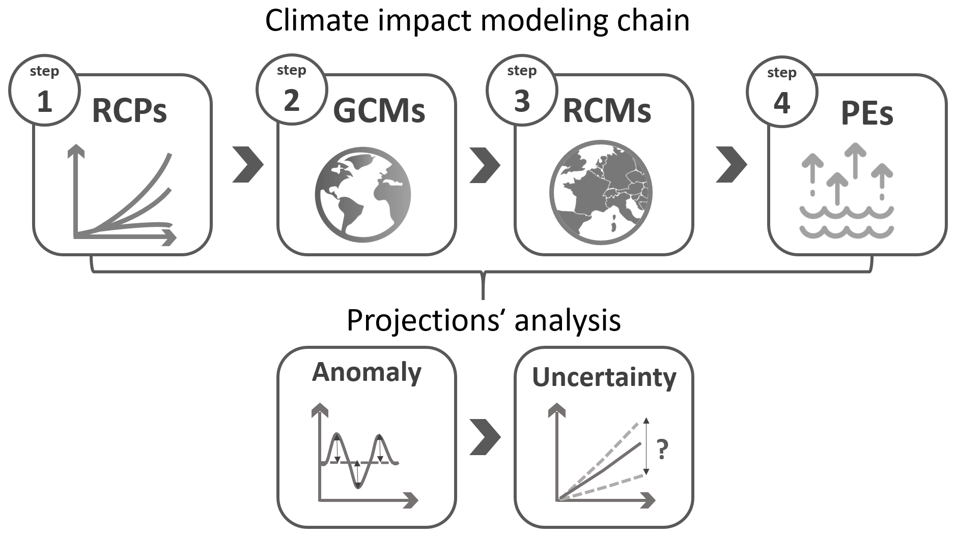
Figure 1Diagram representing the modeling chain for the study of the impact of climate change on potential evaporation.
2.2 PE formulations
Seven PE formulations were selected in this study (see Table 2). This selection was made to represent diverse ways of estimating PE, including physically based methods derived from the energy balance and empirical methods. In this study, all formulations were applied at a daily time step.
Penman (1948)Allen et al. (1998)Monteith (1965)Allen et al. (1998)Priestley and Taylor (1972)Morton (1983)McMahon et al. (2013)Oudin et al. (2005)Hamon (1963)Oudin et al. (2005)Hargreaves and Samani (1985)Allen et al. (1998)Table 2The seven formulations used to compute PE. The “Climate variables” column refers to the input data required in each PE formulation. Rn is net radiation, RH is relative humidity, u2 is 2 m wind speed and Ta is 2 m air temperature. Full equations are available in the provided R code (see the “Code availability” section). The Penman–Monteith method is from FAO 56. The Hamon formulation uses theoretical sunshine hours (Oudin et al., 2005; Almorox et al., 2015). RRM refers to rainfall–runoff modeling.
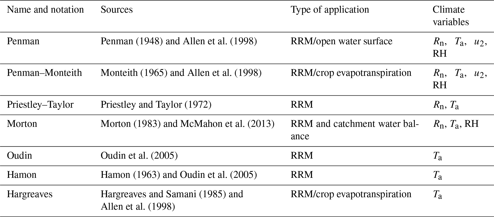
The Penman and Penman–Monteith formulations are often referred to as combinational methods, as they are derived from the energy budget coupled with aerodynamic considerations. While the Penman formulation is recommended for open water evaporation estimation, the Penman–Monteith formulation was proposed to estimate the potential evaporation from a reference crop. These two formulations are widely used in crop water requirement and hydrological models, as they make full use of currently measurable climate variables, under a physically derived framework. For climate change impact studies, these formulations allow one to account for possible interactions and feedbacks between climate variables. The Priestley–Taylor formulation is a simplification of the Penman equation that allows for the estimation of PE with only radiative climate variables. This formulation does not make use of aerodynamic climate variables, which are highly uncertain in climate change impact studies. The Morton formulation was recommended by McMahon et al. (2013) for hydrological modeling. Based on the Priestley–Taylor formulation, it includes an iterative estimation of a so-called equilibrium temperature, which better represents the surface temperature. The Oudin, Hamon and Hargreaves formulations use air temperature only. Proxies of solar radiation are implicitly included in these formulations, either via extraterrestrial radiation estimation or by using empirically derived equations that relate radiation to the mean or amplitude of daily air temperature. For climate change impact studies, these formulations are interesting, as air temperature is probably the least uncertain variable in climate projections. However, the absence of other climate variables is questionable under climate change because feedbacks between climate variables exist, such as the dimming effect causing radiation to decrease while the air temperature increases. Shaw and Riha (2011) pointed out higher future PE amounts with the temperature-based formulations, compared with other formulations, over five predominantly hardwood forest sites at differing latitudes in the eastern United States.
2.3 Quantifying and partitioning projected PE uncertainties
A Bayesian data augmentation technique, the QUALYPSO (Quasi-ergodic AnaLYsis of climate ProjectionS using data augmentatiOn) method (Evin et al., 2019; Evin, 2020), was applied to deal with the lack of balance in terms of representation within the combinations of climate models (GCMs–RCMs) and RCPs (see gaps in Table 1). The data set available for this study is composed of 30 RCP–GCM–RCM chains multiplied by seven PE formulations. The Bayesian data augmentation process of the QUALYPSO framework fills a complete and balanced matrix of climate projections composed of 162 members (3 RCPs × 6 GCMs × 9 RCMs) multiplied by 7 PE formulations. This process results in a balanced data set, which is essential to correctly assess the contribution of each modeling step and to avoid inducing a biased estimation of the variance explained by a specific modeling step being over- or underrepresented. This framework was successfully applied by Lemaitre-Basset et al. (2021) to analyze projected hydrological uncertainties with an incomplete ensemble of projections. Analysis of variance (ANOVA) methods are frequently used to quantify the contribution of different models to total uncertainty. They rely on the respective variance contributions of the different modeling chain steps to the total variance. An ANOVA can be performed with a time series approach, as mentioned by Hingray and Saïd (2014), which considers the quasi-ergodicity of climate variables for the long term. This approach was also used by Lafaysse et al. (2014) and Vidal et al. (2016), who added the downscaling and hydrological modeling steps to the modeling chain in the evaluation of uncertainties. In the present study, to quantify and partition the total uncertainty with respect to the projected changes among the different modeling steps, the quasi-ergodic analysis of variance (QE-ANOVA) framework was chosen (Hingray and Saïd, 2014; Hingray et al., 2019). The QE-ANOVA method allows for the decomposition of the total variance of the projected potential evaporation estimates. The total uncertainty partitioning is composed of the sum of the specific variance of each modeling chain step (namely RCPs, GCMs, RCMs and the PE formulations) as well as a residual term, representing the interaction between models. Moreover, a 30-year rolling mean is applied on projected variables that are available from 1976 to 2099 in order to reduce the impact of internal variability. Within the QE-ANOVA analysis, the trend signal analyzed by a variance decomposition is a trend model fitted to rolling mean projections. This statistical analysis allows for the assessment of the importance of the choice of PE formulation, according to the timescale and geographical-area targets. Finally, a signal-to-noise ratio is used to determine the strength of PE changes over France. The ensemble mean PE expected changes represents the signal, and the noise is represented by the standard deviation between simulations.
3.1 Trends in potential evaporation according to the different RCPs
Figure 2a shows the mean annual PE, from a multi-scenario and multi-model average, over the reference period from 1976 to 2005 based on climate projection data. Across France, a north–south gradient is visible, with the highest values obtained over the Mediterranean region, and the lowest values obtained over the northern part of the country and the mountainous areas (the Alps and Pyrenees).
Annual PE is shown to increase over the 1976–2005 period (Fig. 2b). A mean increase from about 730 mm y−1 at the beginning of the century to about 840 mm y−1 by the end of the century is simulated for all RCPs on average (Fig. 2b). However, this PE increase highly depends on RCPs, as PE reaches around 775, 820 and 920 mm y−1 for RCP2.6, RCP4.5 and RCP8.5, respectively. This means that, for the majority of climate models and PE formulations, the projected increase in greenhouse gas concentrations clearly leads to an increase in PE estimates, and the trend in PE is closely related to the RCP considered: an exponential increase for RCP8.5, a rather linear increase for RCP4.5 and a plateau reached by 2040 for RCP2.6.
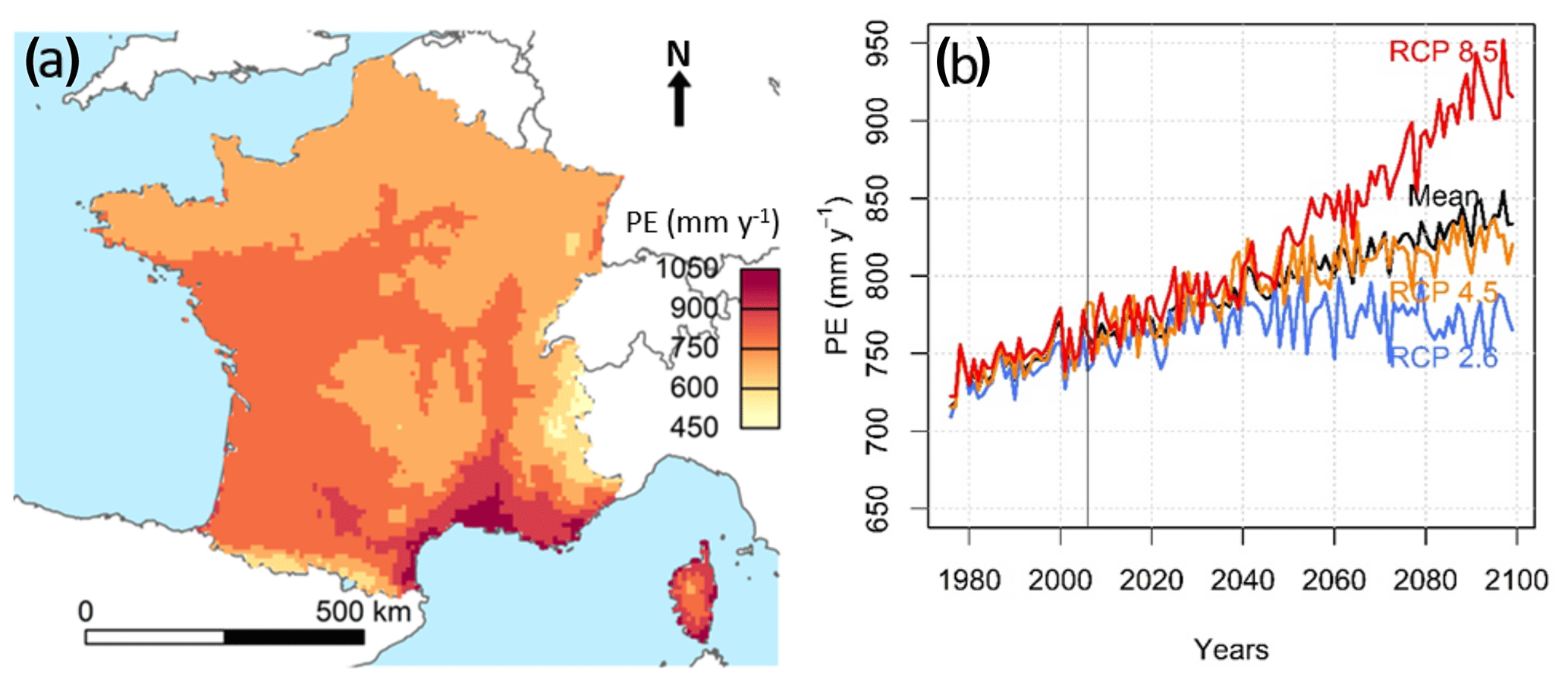
Figure 2(a) Mean annual PE (mm y−1) computed with climate projections from 1976 to 2005 plotted over France, and (b) mean annual time series of PE averaged over the whole study area computed with the three RCPs (1976–2099). Multiyear (a) and annual (b) mean PE values were calculated by averaging the seven PE formulations and also the different GCM–RCM couples. As mentioned in Table 1, the RCP2.6 time series is obtained by averaging 8 × 7 time series (8 GCM–RCM couples and 7 PE formulations), the RCP4.5 time series is obtained by averaging 10 × 7 time series (10 GCM/RCM couples and 7 PE formulations) and the RCP8.5 time series is obtained by averaging 12 × 7 time series (12 GCM–RCM couples and 7 PE formulations).
3.2 Behavioral differences between PE formulations and links to climate variables
The PE formulations show large differences in terms of magnitude, regardless of the time period considered (Fig. 3a). This is in line with previous studies that compared PE amounts depending on the PE formulation (Federer et al., 1996; Kingston et al., 2009). The differences between formulations reach about 400 mm y−1, which is much higher than the expected PE changes over the 1976–2099 period for a given formulation.
Figure 3b shows gradual positive anomalies for each formulation. By the end of the century, the annual PE changes over the 1976–2099 period are between +30 mm y−1 (on average over 30-year periods) with the Morton formulation and +130 mm y−1 with the Hamon formulation, whose relatively high sensitivity to air temperature increase has already been demonstrated for other locations (Duan et al., 2017). However, interestingly, the growth rate does not necessarily depend on the selected forcing variables nor on the type of equation, as Penman, Penman–Monteith and Oudin present similar trend slopes while probably being most different in terms of formulation and the selected forcing variables.

Figure 3Projected mean annual PE (a) and expected increase (b) for each formulation. The time series are obtained by averaging the 30 RCP–GCM–RCM time series for each PE formulation. A 30-year rolling mean is applied so that, for instance, the value for the first year in the plotted time series (at year 1990) corresponds to the PE averaged over the 1976–2005 period.
To better understand this point, we analyzed the link between the PE and climate variables anomalies, regardless of their use in PE formulations. We show that, irrespective of the PE formulation, an increase in air temperature or radiation or a decrease in relative humidity leads to an increase in PE (Fig. 4). The relationships exhibit rather linear behaviors, with higher slopes obtained for the Hamon PE formulation. This suggests that the covariance between climate variables from GCM–RCM couples of models allows for PE formulations that do not make use of all available climate variables to still show consistent evolutions of annual PE. Surprisingly, no clear relationship is observed between the PE and wind speed anomalies. A large discrepancy exists between the GCM–RCM climate models regarding the sign of the evolution of wind speed, suggesting large uncertainties for this variable.
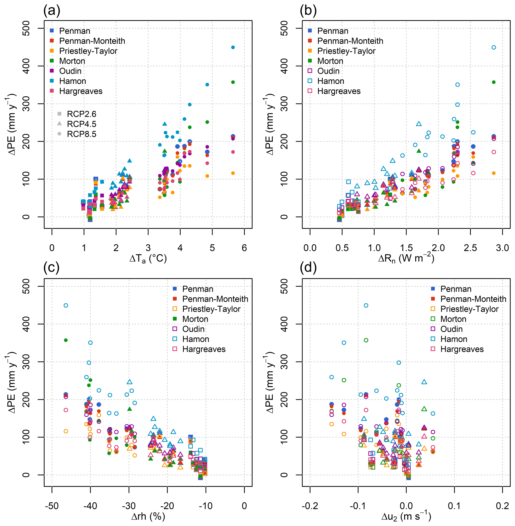
Figure 4Mean anomalies of annual PE compared to the average anomalies of the climate variables by the end of the century (2070–2099) for air temperature (Ta, a), net radiation (Rn, b), relative humidity (RH, c) and wind speed (u2, d). Each symbol represents one combination of RCP–GCM–RCM–PE formulation. Full symbols are used when the climate variable is used in the PE formulation, and blank symbols are used when the climate variable is not used in the PE formulation.
3.3 Quantifying and partitioning the total uncertainty in PE projections
In the previous section, we showed that differences between PE evolutions are large in the future. In this section, we aim to decipher the real contribution of PE formulations to the total uncertainty, relative to other uncertainty contributors (RCPs, GCMs and RCMs). Figure 5 shows the contribution of each modeling step (RCPs, GCMs, RCMs and PE formulations) to the total uncertainty of the future PE changes, i.e., the proportion of the variance explained by each step in the modeling chain for three different 30-year periods centered around 2030, 2050 and 2085, over the entire study domain (France), obtained by applying the QUALYPSO method.
By 2030, GCMs are the main source of uncertainty, with a contribution ranging from 30 % (over the southeastern part of the domain) to 50 % (over the northwest part of the domain). RCMs are the second largest source of uncertainty, with a contribution ranging from 20 % to 30 %. The other steps in the modeling chain exhibit a much lower contribution: PE formulations account for less than 5 % to the total uncertainty, except over the southeastern part of the domain where it reaches 10 %; the RCPs represent less than 10 % of the total uncertainty; and the residual is quite low, with a proportion below 10 %.
By 2050, GCMs are still the largest source of uncertainty over a large part of the territory, with a contribution of about 40 % to the total uncertainty. However, in the southern part of the territory, this contribution is still lower (30 %). The lower contribution of GCMs in this part of the territory can be explained by the increase in the contribution of RCPs to the total uncertainty, by up to 10 % on average. The contributions of RCMs show a small increase in the center of the French territory, from 30 % to 40 % on average. The contributions of other steps remain similar to those for 2030.
By 2085, GCMs and RCMs provide the major sources of uncertainty in the modeling chain, with a respective contribution of 30 %. The contribution of RCPs to the total uncertainty is notably higher than for other periods (especially in the southern part of the domain); thus, in 2085, the divergence between RCP scenarios explains 20 % of the variance in PE estimates. Finally, differences between PE formulations, although they lead to largely different PE changes, remain a minor source of uncertainty compared with other factors, with a contribution to the total uncertainty below 10 %.
The total variance of PE change is the total uncertainty of the PE response to climate change. Interestingly, the total uncertainty increases with time, especially for the southern regions, where the contribution of RCPs is relatively high.
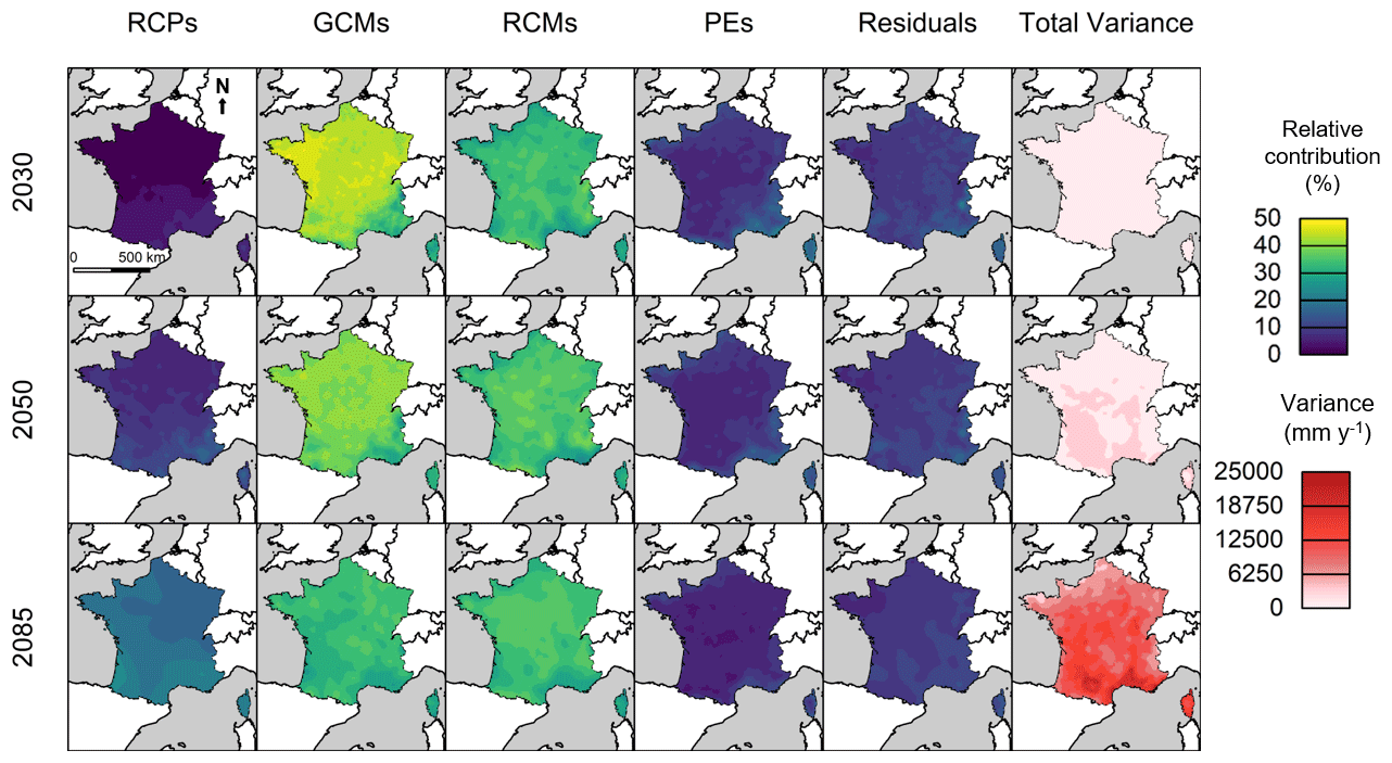
Figure 5Uncertainty contribution of each impact modeling chain step to changes in PE across France for three different 30-year periods centered around 2030, 2050 and 2085. The contribution to the total uncertainty is presented in percent and is calculated with the QUALYPSO method.
3.4 Analyzing the uncertainty in PE projections from a single scenario: RCP8.5
The contribution of PE formulations to the PE projection uncertainty might be underestimated due to the combination of RCPs in the previous analysis. As a consequence, the contribution of PE formulations to the PE projection uncertainty is assessed here for RCP8.5 only. Figure 6 presents the results of the uncertainty analysis for a single scenario: RCP8.5 by 2085. According to the results presented in Fig. 5, the contribution of RCPs becomes higher for the end of the century compared with earlier periods, i.e., when RCPs convey more divergent climate signals with respect to RCP8.5, the total variance (Fig. 6) is moderately smaller than in the multi-scenario analysis (Fig. 5). Therefore, considering multiple RCPs introduces more variability in the long term. Figure 6 shows that the relative contribution of the PE formulations is higher for the analysis considering only RCP8.5 than for the multi-scenario analysis. This is especially the case for the southern locations, where the PE contribution reaches almost 50 % of the variance. GCM and RCM contributions remain stable between the single- and multi-scenario analyses. The results of the uncertainty analysis for a single scenario highlight the important contribution of the PE formulations over the total uncertainty (RCPs excluded), and they even rank the PE formulations as the first uncertainty contributor for the south of France.
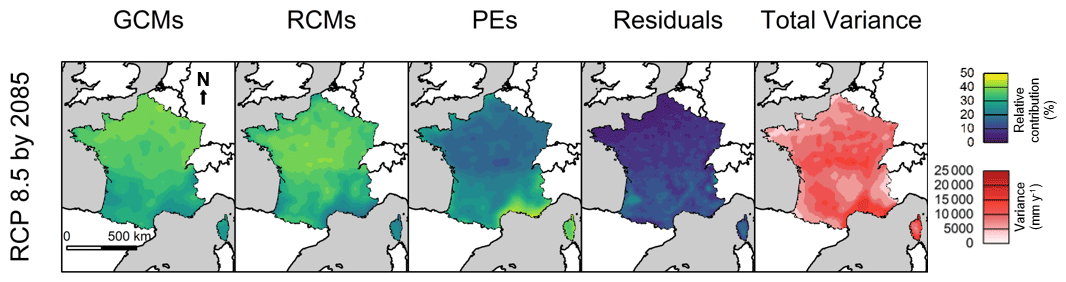
Figure 6Uncertainty contribution of each impact modeling chain step to changes in PE across France for a 30-year period centered around 2085 for RCP8.5. The contribution to the total uncertainty is presented in percent and is calculated with the QUALYPSO method.
The top row of Fig. 7 shows the mean yearly PE increase (mm y−1) for RCP8.5 computed with the complete matrix of data, i.e., completed with the QUALYPSO framework, for three different 30-year periods centered around 2030, 2050 and 2085. The PE increase for future lead times, computed from the inferred complete matrix with the augmentation process, does not modify the spatial distribution of the original data as shown in Fig. 2. The south–north gradient is still well represented for PE anomalies, although mountainous areas no longer stand out.
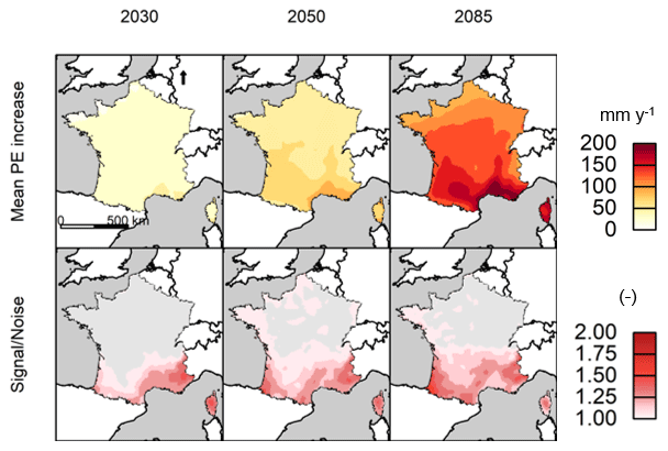
Figure 7The top row shows the mean change in annual PE (mm y−1) computed with the QUALYPSO framework, the bottom row presents the signal-to-noise ratio. Results are shown for three different 30-year periods centered around 2030, 2050 and 2085. Gray areas indicate a signal-to-noise ratio below 1 at the 90 % confidence bounds, whereas red areas show ratios above 1.
Finally, the signal-to-noise ratio due to climate change, based on the method of Hawkins and Sutton (2012), is presented in Fig. 7 (bottom row). This indicator allows one to assess if the change signal is more important than the uncertainty associated with the change trend (i.e., the noise of the ensemble). When the signal-to-noise ratio is above 1, the change is more important than the uncertainty, and an emergence time can be associated with the change trend. The expected increase in PE becomes greater than the variability for the southern areas of the domain, indicating a signal emergence. For northern locations, a large uncertainty is associated with the estimation of future PE.
4.1 Investigating the role of the uncertainty-partitioning approach on results
We performed a descriptive analysis to evaluate the distribution of PE changes, more specifically the distributions of PE anomalies averaged over the entire domain (France) according to each scenario and model. Figure 8 shows the variability of the mean PE anomaly projected over France for each model and scenario used in the study, namely RCPs, GCMs, RCMs and PE formulations, for three different 30-year periods centered around 2030, 2050 and 2085. The figure allows one to identify which scenario or model in the ensemble is likely to convey more uncertainty to the projections. For example, a model showing greater variability than other models or a significantly different projection can be identified as contributing a significant amount to the ensemble uncertainty range. At first glance, Fig. 8 shows an increase in the variability of the projections with time, i.e., a growing uncertainty associated with the PE projections from horizon 2030 to horizon 2085. This increase is relevant to previously shown results, such as the divergence between RCPs (Fig. 2), the divergence between PE formulations (Fig. 3) or the increase in total uncertainty (Fig. 5).
Regarding the RCPs, the divergence between the three pathways increases with time. At the 2085 horizon, PE projections clearly differ according to the emission scenario, which explains the results observed in Fig. 5 (increased proportion of uncertainty due to RCPs). As expected, RCP8.5 shows the largest uncertainty range and mean value increase, followed by RCP4.5 and RCP2.6. Given that the signal-to-noise ratio (in Fig. 7) is calculated from the mean of the total set of projections, we can assume that if only RCP8.5 were considered to estimate future PE, the signal-to-noise ratio would be greater and would be more likely to be above unity for some areas and under some horizons (as shown in Fig. 6), whereas the signal-to-noise ratio would be lower when considering RCP2.6 only.
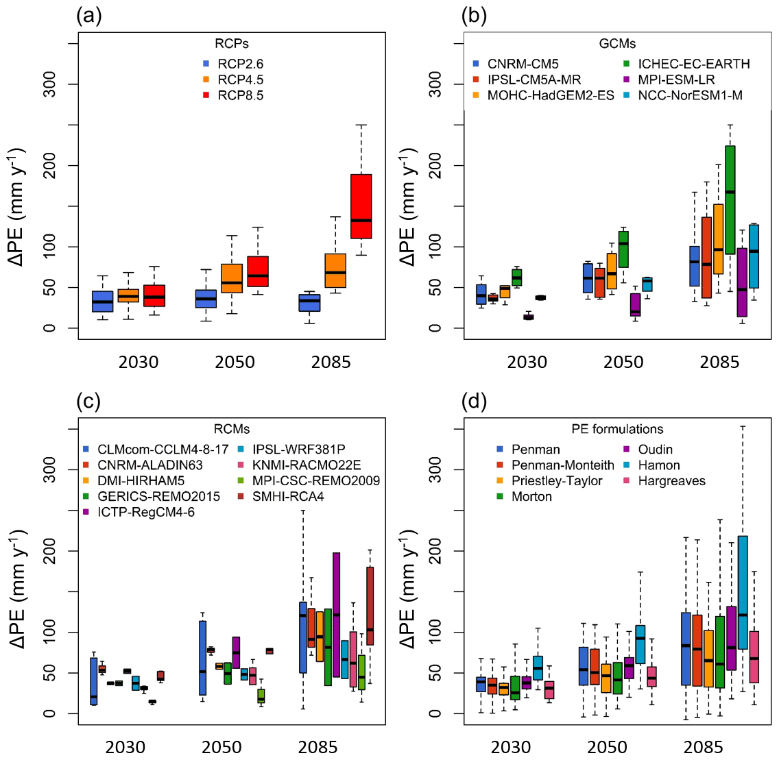
Figure 8Distribution of annual PE changes across France for three different 30-year periods centered around 2030, 2050 and 2085 for each modeling step: RCPs (a), GCMs (b), RCMs (c) and PE formulations (d). The boxplots represent the 5, 25, 50, 75 and 95 quantiles of the distributions. A boxplot provides information on the variability in the PE anomaly for a given modeling step, whereas the other modeling steps vary across their PE anomaly range.
Regarding the GCMs, the divergence of PE projections between each model increases over time in terms of the median change and distributions of change. Moreover, the uncertainty spread also increases with time, which adds up to the total uncertainty, despite the fact that the relative contribution of this factor to the total uncertainty decreases with time (see Fig. 5). Two GCMs stand out from the rest: ICHEC-EC-EARTH projects notably higher PE than the others, whereas MPI-ESM-LR shows significantly lower PE values.
The divergence between RCMs increases over time as well. It must be highlighted that not all RCMs are used with the same GCMs. For example, CLMcom-CCLM4-8-17 appears in Fig. 8 as the RCM with the most variability; however, this RCM only uses the outputs of two different GCMs, the MPI-ESM-LR model that projects the lowest PE increase and the MOHC-HadGEM2-ES model that projects one of the highest PE increases. Thus, the projected higher uncertainty derived from this RCM can be explained by significantly divergent GCM inputs to this model compared with the other RCMs.
Finally, Fig. 8 also shows changes in the PE projection uncertainty level and spread derived from the PE formulations. For each time horizon, the uncertainty level and spread show similar values across the seven PE models. However, for each formula, the variability and, hence, the uncertainty to PE projections increases over time. In addition, it is clear that, except for the Hamon formulation, all PE projection anomalies remain within similar value ranges. This important result confirms that PE formulations are not the main factor of uncertainty in PE projections, compared with RCPs, GCMs and RCMs.
4.2 Guidelines for selecting PE formulations in impact studies
Two related questions arise when using PE data as input for climate change impact models:
-
Do we need to consider multiple PE formulations or does a single PE formulation suffice?
-
Which formulation(s) are preferable?
As for the first question, our results suggest that PE formulations may have different future trends and that assessing these differences using a multi-formulation approach is undoubtedly a relevant practice. The PE anomalies obtained in this study are of the same order of magnitude as those of previous studies, and they rank PE formulations in a similar way (Milly and Dunne, 2016, 2017). However, uncertainty analysis results depend on the framework of the climate impact study: combining multiple scenarios or treating each scenario independently. For the multi-scenario analysis, considering the other sources of uncertainty conveyed by RCPs, GCMs and RCMs, we found that PE formulations account for only around 10 % of the total uncertainty in PE projections. This result contrasts with previous studies that have highlighted the relatively important role of PE formulation in the impact modeling chain (Vidal et al., 2013; Seiller and Anctil, 2016; Williamson et al., 2016). However, we must note that many of these studies focused on the RCP8.5 scenario, which is associated with the highest greenhouse gas emissions and, therefore, the highest radiative forcing. The results of the uncertainty analysis performed for RCP8.5 are more consistent with other studies. This leads to greater divergence between the formulations than in the multi-scenario approach, due to the higher future air temperature gradient. We attribute the differences between our results and those from previous studies to the inclusion of several climate model simulations under a large range of emission scenarios and to the approach used to partition uncertainty (relying on a Bayesian method to complete our unbalanced set of projections). However, another hypothesis that could explain the discrepancy between our results and those from other studies is the use (or not) of bias-corrected data. Using bias-corrected data reduces the contribution of GCMs/RCMs to total uncertainty (as their distributions are forced to match an observed data set), in contrast to using raw data. In this study, we prefer not to include bias-corrected data, as most bias-corrected climate projections with statistical methods perform poorly with respect to retaining the properties of the covarying variables needed for the PE calculation (Vrac and Friederichs, 2015). In addition, in contrast to these studies, we did not use an impact model (such as a hydrological model or a crop water requirement model), as we aimed to make this study as general as possible. Due to the minor contribution of PE formulations to the total uncertainty in PE projections, when multiple scenarios are considered, it does not seem necessary to consider several formulations in multi-scenario climate impact studies. However, for a single-scenario analysis (treating each scenario independently), the contribution of the PE formulation becomes higher, and it seems necessary to quantify this source of uncertainty as well as the GCM and RCM contributions. Furthermore, if several impact models are used, due to the differences in the magnitude of PE and its changes between formulations, the same formulation should be conserved for all modeling chains. These recommendations do not apply if only one climate projection is used, which should be avoided anyway.
As for the second question, it is difficult to provide clear guidelines. In theory, the choice of a PE formulation for an impact study needs to consider both the uncertainties with respect to the projected climate variables used by the formulations and the physical consistency handled by these formulations. In practice, as the choice of a PE formulation is often driven by the personal experience of the modeler, the relatively low contribution of PE formulations in multi-scenario analysis, relative to other sources of uncertainty, tends to confirm this practice. We showed that the behaviors of the PE formulations along projected climatic gradients are generally consistent (Fig. 4), even for very different formulations in terms of the climate variables used and physical consistency. This results from the fact that other climate variables covary with temperature, and these relationships are maintained in climate projections. If one wants to take other aspects into account, such as CO2, we would recommend choosing a Penman–Monteith-type formula that explicitly allows for this. We found that Penman–Monteith PE trends are close to the average of the PE formulations tested. Moreover, the physical soundness of this method allows one to more explicitly account for interactions between climate drivers than other formulations (even though we showed that those interactions tend to be implicitly taken into account in all formulations). In addition, its structure theoretically allows one to consider other environmental changes, such as land use or plant behavior under elevated atmospheric CO2, in a more explicit way (Schwingshackl et al., 2019; Yang et al., 2019). Accounting for these changes probably represents a greater challenge than identifying the “best” PE formulation with fixed vegetation parameters.
4.3 Implications of evaporation uncertainties in impact studies
This paper has tackled the issue of uncertainty in PE projections, but PE is only a modeling result. Here, we discuss how PE uncertainty is transferred to actual evaporation (AE) uncertainty. Generally, AE is computed as a fraction of PE, typically constrained by soil moisture. How uncertainty in PE propagates to AE depends on the region. In water-limited regions (such as in the Mediterranean region in our study), the impact of PE uncertainty on the AE estimate is negligible. However, the precipitation projections have a large uncertainty, which affects the estimated AE in such regions. Indeed, an increasing (decreasing) trend of precipitation results in increased (decreased) soil moisture and, thus, AE. In energy-limited regions, the uncertainty of PE is more important than the uncertainty of precipitation to estimate long-term AE.
This leads one to question the sensitivity of impact models to PE variability. Numerous rainfall–runoff models employed for impact studies use PE as input. The representation of the evaporation process in the model may have consequences for the transfer of uncertainties. For example, the HBV (Hydrologiska Byråns Vattenbalansavdelning) model considers AE to be equal to PE if soil moisture is sufficient; if not, AE is reduced to satisfy the previous condition, which could reduce the PE uncertainty (Seibert and Vis, 2012). Calibrated hydrological models can accommodate errors in PE estimates (Oudin et al., 2006) but are much more sensitive if the errors are not constant over time (Nandakumar and Mein, 1997). The optimization of any hydrological model parameters with observed streamflow data might compensate for errors and uncertainty with respect to PE. This becomes an issue for the extrapolation period, where the risk is to project excessive dry or wet future conditions under climate change. While the equations described in this paper are used for rainfall–runoff models and, thus, for hydrological climate impact studies, they are not necessarily appropriate for crop water requirements, as crop-specific parameters might be considered. For such a purpose, the set of PE formulations should represent vegetation parameters, which could lead to different evolutions than the set of formulations chosen in this study. Crop-specific parameters are indeed susceptible to be sensitive to aspects other than the climatic variables tested in our study, which might modify the uncertainty contribution.
Potential evaporation (PE) is a necessary proxy for the estimation of actual evaporation in impact models, such as hydrological and crop water requirement models. However, many formulations exist, and the role of these formulations in projections remains largely unclear. In this study, we investigated the uncertainty sources of PE projections using 30 RCP–GCM–RCM combinations and seven PE formulations over the 21st century. Using an ANOVA-based method, we assessed the contribution of each step of the PE modeling chain to the PE uncertainty.
Our work shows that, regardless the PE formulation used, the mean PE will increase across France (from +40 to 130 mm y−1 on average over 30-year periods), with higher increases associated with a higher greenhouse gas emission scenario. The PE increase is higher in the southern part of France and lower in the northern part. Moreover, uncertainties are large, leading to a signal-to-noise ratio that is higher than 1 for southern locations and below 1 for northern locations. This results in issues with determining an emergence time in terms of signal change for the entire domain. The contribution of the PE formulations to the overall uncertainty in PE projections is much lower than the contribution of the other uncertainty sources (namely RCPs, GCMs and RCMs) in a multi-scenario approach. On the other hand, in a single-scenario analysis, using RCP8.5, the contribution of the evaporation formulations becomes higher and even dominant for the southern part of France. However, this work also highlighted differences, both in terms of absolute values and future changes, in PE among the different formulations. The divergence between formulations was found to be higher with higher air temperature increases. The Hamon formulation leads to the highest increase, whereas the Morton formulation leads to the smallest increase.
Finally, the ranking of formulations (according to magnitude) does not change over time, and the quantification of the PE uncertainty contribution should depend of the framework single scenario or multiple scenarios. However, the bias induced by the formulation could lead to a different estimation depending on the impact modeling chain used. Further work may consider testing these conclusions using a full climate impact modeling chain, for example, including an integrated hydrological model, which would have a different sensitivity to PE.
The PE formulation codes can be retrieved from https://doi.org/10.15454/NCNCHG (Lemaitre-Basset, 2021).
EURO-CORDEX data can be accessed via different European data nodes; see https://www.euro-cordex.net (EURO-CORDEX, 2022).
TLB, LO, GT, and LC conceived the experimental setup. TLB performed the calculations and analysis and wrote the first version of the paper. TLB, LO, GT, and LC contributed to the final version of the paper.
The contact author has declared that neither they nor their co-authors have any competing interests.
Publisher’s note: Copernicus Publications remains neutral with regard to jurisdictional claims in published maps and institutional affiliations.
The authors acknowledge Météo-France for preparing the EURO-CORDEX climate projections, which are projected on an 8 km resolution grid for all CMIP5 models. The first author was funded by Sorbonne University and by Agence de l'Eau Rhin-Meuse.
This research has been supported by Agence de l'eau Rhin-Meuse (grant no. REG-2020-00735) and Sorbonne University (grant no. 3552/2019).
This paper was edited by Markus Hrachowitz and reviewed by two anonymous referees.
Allen, R. G., Pereira, L. S., Raes, D., and Smith, M.: FAO Irrigation and drainage paper, Rome: Food and Agriculture Organization of the United Nations, 56, 1998. a, b, c, d
Almorox, J., Quej, V. H., and Martí, P.: Global performance ranking of temperature-based approaches for evapotranspiration estimation considering Köppen climate classes, J. Hydrol., 528, 514–522, https://doi.org/10.1016/j.jhydrol.2015.06.057, 2015. a
Bae, D.-H., Jung, I.-W., and Lettenmaier, D. P.: Hydrologic uncertainties in climate change from IPCC AR4 GCM simulations of the Chungju Basin, Korea, J. Hydrol., 401, 90–105, https://doi.org/10.1016/j.jhydrol.2011.02.012, 2011. a
Boé, J. and Terray, L.: Uncertainties in summer evapotranspiration changes over Europe and implications for regional climate change, Geophys. Res. Lett., 35, L05702, https://doi.org/10.1029/2007GL032417, 2008. a
Dallaire, G., Poulin, A., Arsenault, R., and Brissette, F.: Uncertainty of potential evapotranspiration modelling in climate change impact studies on low flows in North America, Hydrolog. Sci. J., 66, 689–702, https://doi.org/10.1080/02626667.2021.1888955, 2021. a
Donohue, R. J., McVicar, T. R., and Roderick, M. L.: Assessing the ability of potential evaporation formulations to capture the dynamics in evaporative demand within a changing climate, J. Hydrol., 386, 186–197, https://doi.org/10.1016/j.jhydrol.2010.03.020, 2010. a
Duan, K., Sun, G., McNulty, S. G., Caldwell, P. V., Cohen, E. C., Sun, S., Aldridge, H. D., Zhou, D., Zhang, L., and Zhang, Y.: Future shift of the relative roles of precipitation and temperature in controlling annual runoff in the conterminous United States, Hydrol. Earth Syst. Sci., 21, 5517–5529, https://doi.org/10.5194/hess-21-5517-2017, 2017. a
EURO-CORDEX: https://www.euro-cordex.net, last access: 19 April 2022. a
Evin, G.: QUALYPSO: Partitioning Uncertainty Components of an Incomplete Ensemble of Climate Projections, R package version 1.2, https://CRAN.R-project.org/package=QUALYPSO, last access: 5 December 2020. a
Evin, G., Hingray, B., Blanchet, J., Eckert, N., Morin, S., and Verfaillie, D.: Partitioning Uncertainty Components of an Incomplete Ensemble of Climate Projections Using Data Augmentation, J. Climate, 32, 2423–2440, https://doi.org/10.1175/jcli-d-18-0606.1, 2019. a
Federer, C. A., Vörösmarty, C., and Fekete, B.: Intercomparison of Methods for Calculating Potential Evaporation in Regional and Global Water Balance Models, Water Resour. Res., 32, 2315–2321, https://doi.org/10.1029/96WR00801, 1996. a
Hamon, W. R.: Estimating Potential Evapotranspiration, T. Am. Soc. Civ. Eng., 128, 324–338, https://doi.org/10.1061/TACEAT.0008673, 1963. a
Hargreaves, H. G. and Samani, A. Z.: Reference Crop Evapotranspiration from Temperature, Appl. Eng. Agric., 1, 96–99, https://doi.org/10.13031/2013.26773, 1985. a
Hawkins, E. and Sutton, R.: Time of emergence of climate signals, Geophys. Res. Lett., 39, https://doi.org/10.1029/2011GL050087, 2012. a
Hingray, B. and Saïd, M.: Partitioning Internal Variability and Model Uncertainty Components in a Multimember Multimodel Ensemble of Climate Projections, J. Climate, 27, 6779–6798, https://doi.org/10.1175/JCLI-D-13-00629.1, 2014. a, b
Hingray, B., Blanchet, J., Evin, G., and Vidal, J.-P.: Uncertainty component estimates in transient climate projections, Clim. Dynam., 53, 2501–2516, https://doi.org/10.1007/s00382-019-04635-1, 2019. a
Hosseinzadehtalaei, P., Tabari, H., and Willems, P.: Quantification of uncertainty in reference evapotranspiration climate change signals in Belgium, Hydrol. Res., 48, 1391–1401, https://doi.org/10.2166/nh.2016.243, 2016. a
Intergovernmental Panel on Climate Change: Climate Change 2013 – The Physical Science Basis: Working Group I Contribution to the Fifth Assessment Report of the Intergovernmental Panel on Climate Change, Cambridge University Press, Cambridge, UK, https://doi.org/10.1017/CBO9781107415324, 2014a. a
Intergovernmental Panel on Climate Change: Technical Summary, Cambridge University Press, 1, 35–94, https://doi.org/10.1017/CBO9781107415379.004, 2014b. a
Jacob, D., Petersen, J., Eggert, B., Alias, A., Christensen, O. B., Bouwer, L. M., Braun, A., Colette, A., Deque, M., Georgievski, G., Georgopoulou, E., Gobiet, A., Menut, L., Nikulin, G., Haensler, A., Hempelmann, N., Jones, C., Keuler, K., Kovats, S., Kroner, N., Kotlarski, S., Kriegsmann, A., Martin, E., Van Meijgaard, E., Moseley, C., Pfeifer, S., Preuschmann, S., Radermacher, C., Radtke, K., Rechid, D., Rounsevell, M., Samuelsson, P., Somot, S., Soussana, J.-F., Teichmann, C., Valentini, R., Vautard, R., Weber, B., and Yiou, P.: EURO-CORDEX: new high-resolution climate change projections for European impact research, Reg. Environ. Change, 14, 563–578, https://doi.org/10.1007/s10113-013-0499-2, 2014. a
Jung, M., Reichstein, M., Ciais, P., Seneviratne, S.I., Sheffield, J., Goulden, M.L., Bonan, G., Cescatti, A., Chen, J., de Jeu, R., Dolman, A.J., Eugster, W., Gerten, D., Gianelle, D., Gobron, N., Heinke, J., Kimball, J., Law, B.E., Montagnani, L., Mu, Q., Mueller, B., Oleson, K., Papale, D., Richardson, A.D., Roupsard, O., Running, S., Tomelleri, E., Viovy, N., Weber, U., Williams, C., Wood, E., Zaehle, S., and Zhang, K.: Recent decline in the global land evapotranspiration trend due to limited moisture supply, Nature, 467, 951–954, https://doi.org/10.1038/nature09396, 2010. a
Kay, A. and Davies, H.: Calculating potential evaporation from climate model data: A source of uncertainty for hydrological climate change impacts, J. Hydrol., 358, 221–239, https://doi.org/10.1016/j.jhydrol.2008.06.005, 2008. a, b, c, d
Kingston, D. G., Todd, M. C., Taylor, R. G., Thompson, J. R., and Arnell, N. W.: Uncertainty in the estimation of potential evapotranspiration under climate change, Geophys. Res. Lett., 36, L20403, https://doi.org/10.1029/2009GL040267, 2009. a
Koedyk, L. P. and Kingston, D. G.: Potential evapotranspiration method influence on climate change impacts on river flow: a mid-latitude case study, Hydrol. Res., 47, 951–963, https://doi.org/10.2166/nh.2016.152, 2016. a, b, c, d, e
Lafaysse, M., Hingray, B., Mezghani, A., Gailhard, J., and Terray, L.: Internal variability and model uncertainty components in future hydrometeorological projections: The Alpine Durance basin, Water Resour. Res., 50, 3317–3341, https://doi.org/10.1002/2013WR014897, 2014. a
Lemaitre-Basset, T.: R functions to compute potential evaporation, Portail Data INRAE [data set], https://doi.org/10.15454/NCNCHG, 2021. a
Lemaitre-Basset, T., Collet, L., Thirel, G., Parajka, J., Evin, G., and Hingray, B.: Climate change impact and uncertainty analysis on hydrological extremes in a French Mediterranean catchment, Hydrolog. Sci. J., 66, 888–903, https://doi.org/10.1080/02626667.2021.1895437, 2021. a
McAfee, S. A.: Methodological differences in projected potential evapotranspiration, Climatic Change, 120, 915–930, https://doi.org/10.1016/0168-1923(93)90095-Y, 2013. a
McKenney, M. S. and Rosenberg, N. J.: Sensitivity of some potential evapotranspiration estimation methods to climate change, Agr. Forest Meteorol., 64, 81–110, https://doi.org/10.1016/0168-1923(93)90095-Y, 1993. a
McMahon, T. A., Peel, M. C., Lowe, L., Srikanthan, R., and McVicar, T. R.: Estimating actual, potential, reference crop and pan evaporation using standard meteorological data: a pragmatic synthesis, Hydrol. Earth Syst. Sci., 17, 1331–1363, https://doi.org/10.5194/hess-17-1331-2013, 2013. a, b
Milly, P. and Dunne, K. A.: A Hydrologic Drying Bias in Water-Resource Impact Analyses of Anthropogenic Climate Change, J. Am. Water Resour. As., 53, 822–838, https://doi.org/10.1111/1752-1688.12538, 2017. a, b, c, d, e
Milly, P. C. and Dunne, K. A.: Potential evapotranspiration and continental drying, Nat. Clim. Change, 6, 946–949, https://doi.org/10.1038/nclimate3046, 2016. a, b, c
Monteith, J. L.: Evaporation and environment, in: Symposia of the society for experimental biology, volume 19, Cambridge University Press (CUP), Cambridge, UK, 205–234 pp., 1965. a
Morton, F.: Operational estimates of areal evapotranspiration and their significance to the science and practice of hydrology, J. Hydrol., 66, 1–76, https://doi.org/10.1016/0022-1694(83)90177-4, 1983. a
Nandakumar, N. and Mein, R.: Uncertainty in rainfall—runoff model simulations and the implications for predicting the hydrologic effects of land-use change, J. Hydrol., 192, 211–232, https://doi.org/10.1016/S0022-1694(96)03106-X, 1997. a
Oudin, L., Hervieu, F., Michel, C., Perrin, C., Andréassian, V., Anctil, F., and Loumagne, C.: Which potential evapotranspiration input for a lumped rainfall–runoff model?: Part 2—Towards a simple and efficient potential evapotranspiration model for rainfall–runoff modelling, J. Hydrol., 303, 290–306, https://doi.org/10.1016/j.jhydrol.2004.08.026, 2005. a, b, c
Oudin, L., Perrin, C., Mathevet, T., Andréassian, V., and Michel, C.: Impact of biased and randomly corrupted inputs on the efficiency and the parameters of watershed models, J. Hydrol., 320, 62–83, https://doi.org/10.1016/j.jhydrol.2005.07.016, 2006. a
Penman, H. L.: Natural evaporation from open water, bare soil and grass, P. Roy. Soc. Lond. A. Mat., 193, 120–145, https://doi.org/10.1098/rspa.1948.0037, 1948. a
Priestley, C. H. B. and Taylor, R. J.: On the Assessment of Surface Heat Flux and Evaporation Using Large-Scale Parameters, Mon. Weather Rev., 100, 81–92, https://doi.org/10.1175/1520-0493(1972)100<0081:OTAOSH>2.3.CO;2, 1972. a
Prudhomme, C. and Williamson, J.: Derivation of RCM-driven potential evapotranspiration for hydrological climate change impact analysis in Great Britain: a comparison of methods and associated uncertainty in future projections, Hydrol. Earth Syst. Sci., 17, 1365–1377, https://doi.org/10.5194/hess-17-1365-2013, 2013. a
Schwingshackl, C., Davin, E. L., Hirschi, M., Sørland, S. L., Wartenburger, R., and Seneviratne, S. I.: Regional climate model projections underestimate future warming due to missing plant physiological CO2 response, Environ. Res. Lett., 14, 114019, https://doi.org/10.1088/1748-9326/ab4949, 2019. a
Seibert, J. and Vis, M. J. P.: Teaching hydrological modeling with a user-friendly catchment-runoff-model software package, Hydrol. Earth Syst. Sci., 16, 3315–3325, https://doi.org/10.5194/hess-16-3315-2012, 2012. a
Seiller, G. and Anctil, F.: How do potential evapotranspiration formulas influence hydrological projections?, Hydrolog. Sci. J., 61, 2249–2266, https://doi.org/10.1080/02626667.2015.1100302, 2016. a, b
Shaw, S. B. and Riha, S. J.: Assessing temperature-based PET equations under a changing climate in temperate, deciduous forests, Hydrol. Process., 25, 1466–1478, https://doi.org/10.1002/hyp.7913, 2011. a
Thompson, J., Green, A., and Kingston, D.: Potential evapotranspiration-related uncertainty in climate change impacts on river flow: An assessment for the Mekong River basin, J. Hydrol., 510, 259–279, https://doi.org/10.1016/j.jhydrol.2013.12.010, 2014. a
Vidal, J.-P., Tilmant, F., and Hingray, B.: Uncertainties in changes in potential evaporation: the formulation issue, in: EGU General Assembly 2013, April 2013, Vienna, Austria, 1, https://hal.inrae.fr/hal-02598484 (last access: 27 April 2022), 2013. a, b, c
Vidal, J.-P., Hingray, B., Magand, C., Sauquet, E., and Ducharne, A.: Hierarchy of climate and hydrological uncertainties in transient low-flow projections, Hydrol. Earth Syst. Sci., 20, 3651–3672, https://doi.org/10.5194/hess-20-3651-2016, 2016. a
Vrac, M. and Friederichs, P.: Multivariate—Intervariable, Spatial, and Temporal—Bias Correction, J. Climate, 28, 218–237, https://doi.org/10.1175/JCLI-D-14-00059.1, 2015. a
Wang, W., Xing, W., and Shao, Q.: How large are uncertainties in future projection of reference evapotranspiration through different approaches?, J. Hydrol., 524, 696–700, https://doi.org/10.1016/j.jhydrol.2015.03.033, 2015. a
Wilby, R. L. and Dessai, S.: Robust adaptation to climate change, Weather, 65, 180–185, https://doi.org/10.1002/wea.543, 2010. a
Williamson, T. N., Nystrom, E. A., and Milly, P. C.: Sensitivity of the projected hydroclimatic environment of the Delaware River basin to formulation of potential evapotranspiration, Climatic Change, 139, 215–228, 2016. a, b
Yang, Y., Roderick, M. L., Zhang, S., McVicar, T. R., and Donohue, R. J.: Hydrologic implications of vegetation response to elevated CO2 in climate projections, Nat. Clim. Change, 9, 44–48, 2019. a