the Creative Commons Attribution 4.0 License.
the Creative Commons Attribution 4.0 License.
 | 12 Apr 2022
A combined use of in situ and satellite-derived observations to characterize surface hydrology and its variability in the Congo River basin
Benjamin Kitambo
Fabrice Papa
Adrien Paris
Raphael M. Tshimanga
Stephane Calmant
Ayan Santos Fleischmann
Frederic Frappart
Melanie Becker
Mohammad J. Tourian
Catherine Prigent
Johary Andriambeloson
The Congo River basin (CRB) is the second largest river system in the world, but its hydroclimatic characteristics remain relatively poorly known. Here, we jointly analyse a large record of in situ and satellite-derived observations, including a long-term time series of surface water height (SWH) from radar altimetry (a total of 2311 virtual stations) and surface water extent (SWE) from a multi-satellite technique, to characterize the CRB surface hydrology and its variability. First, we show that SWH from altimetry multi-missions agrees well with in situ water stage at various locations, with the root mean square deviation varying from 10 cm (with Sentinel-3A) to 75 cm (with European Remote Sensing satellite-2). SWE variability from multi-satellite observations also shows a plausible behaviour over a ∼25-year period when evaluated against in situ observations from the subbasin to basin scale. Both datasets help to better characterize the large spatial and temporal variability in hydrological patterns across the basin, with SWH exhibiting an annual amplitude of more than 5 m in the northern subbasins, while the Congo River main stream and Cuvette Centrale tributaries vary in smaller proportions (1.5 to 4.5 m). Furthermore, SWH and SWE help illustrate the spatial distribution and different timings of the CRB annual flood dynamic and how each subbasin and tributary contribute to the hydrological regime at the outlet of the basin (the Brazzaville/Kinshasa station), including its peculiar bimodal pattern. Across the basin, we estimate the time lag and water travel time to reach the Brazzaville/Kinshasa station to range from 0–1 month in its vicinity in downstream parts of the basin and up to 3 months in remote areas and small tributaries. Northern subbasins and the central Congo region contribute highly to the large peak in December–January, while the southern part of the basin supplies water to both hydrological peaks, in particular to the moderate one in April–May. The results are supported using in situ observations at several locations in the basin. Our results contribute to a better characterization of the hydrological variability in the CRB and represent an unprecedented source of information for hydrological modelling and to study hydrological processes over the region.
- Article
(24561 KB) - Full-text XML
- BibTeX
- EndNote


The Congo River basin (CRB) is located in the equatorial region of Africa (Fig. 1). It is the second largest river system in the world, both in terms of drainage area and discharge. The basin covers km2, and its mean annual flow rate is about 40 500 m3 s−1 (Laraque et al., 2009, 2013). It plays a crucial role in the local, regional, and global hydrological and biogeochemical cycles, with significant influence on the regional climate variability (Nogherotto et al., 2013; Burnett et al., 2020). The CRB is indeed one of the three main convective centres in the tropics (Hastenrath, 1985) and receives an average annual rainfall of around 1500 mm yr−1. Additionally, about 45 % of the CRB land area is covered by dense tropical forest (Verhegghen et al., 2012), accounting for ∼20 % of the global tropical forest and storing about t of carbon, equivalent to ∼2.5 years of current global anthropogenic emissions (Verhegghen et al., 2012; Dargie et al., 2017; Becker et al., 2018). The CRB is also characterized by a large network of rivers, along with extensive floodplains and wetlands, such as in the Lualaba region in the southeastern part of the basin and the well-known Cuvette Centrale region (Fig. 1). The CRB rainforest and inland waters therefore strongly contribute to the carbon cycle of the basin (Dargie et al., 2017; Fan et al., 2019; Hastie et al., 2021). Additionally, more than 80 % of the human population within the CRB rely on the basin water resources for their livelihood and are particularly vulnerable to climate variability and alteration and to any future changes that would occur in the basin water cycle (Inogwabini, 2020). Increasing evidence suggest that changes in land use practices, such as large-scale mining or deforestation, pose a significant threat to the basin water resources availability, including hydrological, ecological, and geomorphological processes in the basin (Bele et al., 2010; Ingram et al., 2011; Nogherotto et al., 2013; Tshimanga and Hughes, 2012; Plisnier et al., 2018). These environmental alterations require a better comprehension of the overall basin hydrology across scales. Surprisingly, despite its major importance, the CRB is still one of the least studied river basins in the world (Laraque et al., 2020) and has not attracted as much attention among the scientific communities as, for instance, the Amazon Basin (Alsdorf et al., 2016). Therefore, there is still insufficient knowledge of the CRB hydro-climatic characteristics and processes and their spatiotemporal variability. This is sustained by the lack of comprehensive and maintained in situ data networks that keep the basin poorly monitored at a large scale, therefore limiting our understanding of the major factors controlling freshwater dynamics at proper space- and timescales.
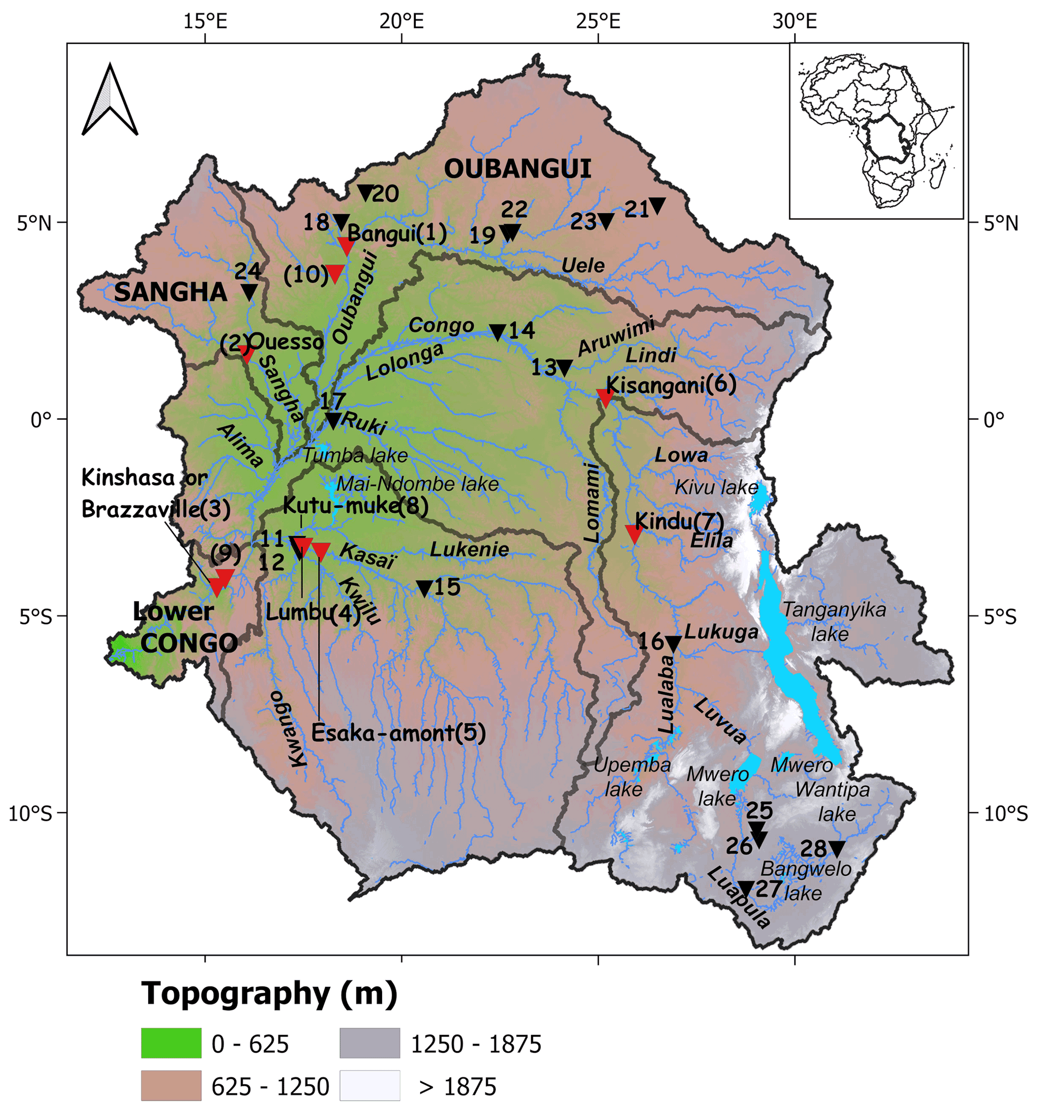
Figure 1The Congo River basin (CRB). Its topography is derived from the Multi-Error-Removed Improved Terrain (MERIT) digital elevation model (DEM), showing the major subbasins (brown line), major rivers, and tributaries. Also displayed are the locations of the in situ gauging stations (triangle). Red and black triangles represent, respectively, the gauge stations with current (>1994) and historical observations. Their characteristics are reported in Table 1.
Efforts have been carried out to undertake studies using remote sensing and/or numerical modelling to overcome the lack of observational information in the CRB and better characterize the various components of the hydrological cycle (Rosenqvist and Birkett, 2002; Lee et al., 2011; Becker et al., 2014; Becker et al., 2018; Ndehedehe et al., 2019; Crowhurst et al., 2020; Fatras et al., 2021; Frappart et al., 2021a). For instance, seasonal flooding dynamics, water level variations, and vegetation types over the CRB were derived from JERS-1 (Rosenqvist and Birkett, 2002) or ALOS PALSAR synthetic aperture radar (SAR) data, as well as ICESat and Envisat altimetry (Betbeder et al., 2014; Kim et al., 2017). Bwangoy et al. (2010) and Betbeder et al. (2014) used combinations of the SAR L band and optical images to characterize the Cuvette Centrale land cover. They found that the wetland extent reaches 360 000 km2 (i.e. 32 % of the total area). Becker et al. (2014) demonstrated the potential of using radar altimetry water levels from Envisat (140 virtual stations – VSs) to classify groups of hydrologically similar catchments in the CRB. Becker et al. (2018) combined information based on Global Inundation Extent from Multi-satellite (GIEMS; Prigent et al., 2007) and altimetry-derived water levels from Envisat (350 VSs) to estimate surface water storage and analyse its variability over the period 2003–2007. Its mean annual variation was estimated at km3, which accounts for 19±5 % of the annual variations in GRACE-derived total terrestrial water storage. Ndehedehe et al. (2019), using the observed Standardized Precipitation Index (SPI) and the global sea surface temperature, examined the impact of the multi-scale ocean–atmosphere phenomena on hydro-climatic extremes, showing that 40 % of the basin during 1994–2006 was affected by severe multi-year droughts. Recently, Fatras et al. (2021) analysed the hydrological dynamics of the CRB using inundation extent estimates from the multi-angular and dual polarization passive L-band microwave signals from the Soil Moisture and Ocean Salinity (SMOS) satellite along with precipitation for 2010–2017. The mean flooded area was found to be 2.39 % for the entire basin, and the dataset helped to characterize floods and droughts during the last 10 years.
In addition to remote sensing observations, hydrological modelling represents a valuable tool for studying the CRB water cycle (Tshimanga et al., 2011; Tshimanga and Hughes, 2014; Aloysius and Saiers, 2017; Munzimi et al., 2019; O'Loughlin et al., 2019; Paris et al., 2022; Datok et al., 2022). For example, Tshimanga and Hughes (2014) used a semi-distributed rainfall–runoff model to examine runoff generation processes and the impact of future climate and land use changes on water resources availability. The magnitude and timing of high and low flows were adequately captured, with, nevertheless, an additional wetland submodel component that was added to the main model to account for wetland and natural reservoir processes in the basin. Aloysius and Saiers (2017) simulated the variability in runoff, in the near future (2016–2035) and mid-century (2046–2065), using a hydrological model forced with precipitation and temperature projections from 25 global climate models (GCMs) under two scenarios of greenhouse gas emission. Munzimi et al. (2019) applied the Geospatial Streamflow Model (GeoSFM) coupled to remotely sensed data to estimate daily river discharge over the basin from 1998 to 2012, revealing a good agreement with the observed flow but also a discrepancy in some parts of the basin where wetland and lake processes are predominant. O'Loughlin et al. (2019) forced the large-scale LISFLOOD-FP hydraulic model with combined in situ and modelled discharges to understand the Congo River's unique bimodal flood pulse. The model was set for the area between Kisangani and Kinshasa on the main stem, including the major tributaries and the Cuvette Centrale region. The results revealed that the bimodal annual pattern is predominantly a hydrological rather than a hydraulically controlled feature. Paris et al. (2022) demonstrated the possibility of monitoring the hydrological variables in near-real time using the hydrologic–hydrodynamic model MGB (Portuguese acronym for large basin model) coupled to the current operational satellite altimetry constellation. The model outputs showed a good consistency with the small number of available observations, yet with some notable inconsistencies in the mostly ungauged Cuvette Centrale region and in the southeastern lakes' subbasins. Datok et al. (2022) used the Soil and Water Assessment Tool (SWAT) model to understand the role of the Cuvette Centrale region in water resources and ecological services. Their findings have highlighted the important regulatory function of the Cuvette Centrale region, which receives contributions from the upstream Congo River (33 %), effective precipitation inside the Cuvette Centrale region (31 %), and other tributaries (36 %).
Most of the above studies based on remote sensing (RS) and hydrological modelling were validated or evaluated against information from other hydrological RS data and/or a few historical gauge data, often enabling only comparisons of seasonal signals (Becker et al., 2018), which also did not cover the same period of data availability (Paris et al., 2022). Therefore, the large size of the basin, its spatial heterogeneity, and the lack of in situ observations have made the validation of long-term satellite-derived observations of surface hydrology components and the proper set-up of large-scale hydrological models difficult (Munzimi et al., 2019). Recent results call for the need of a comprehensive spatial coverage of the CRB water surface elevation using satellite-altimetry-derived observations to encompass the full range of variability across its rivers and wetlands up to its outlet (Carr et al., 2019). Additionally, even if recent efforts have been characterizing how water flows across the CRB, the basin-scale dynamics are still understudied, especially regarding the contributions of the different subbasins to the entire basin hydrology (Alsdorf et al., 2016; Laraque et al., 2020) and to the annual bimodal pattern in the CRB river discharge near to its mouth. Up to now, only a few studies have examined the various contributions and the water transfer from upstream to downstream the basin based on a few in situ discharge gauge records (Bricquet, 1993; Laraque et al., 2020) and large-scale modelling (Paris et al., 2022).
The aim of this study is therefore twofold. First, we provide, for the very first time, an intensive and comprehensive validation of long-term remote-sensing-derived products over the entire CRB, in particular radar altimetry water level variations (a total of 2311 VSs over the period of 1995 to 2020) and surface water extent from multi-satellite techniques from 1992 to 2015 (GIEMS-2; Prigent et al., 2020), using an unprecedented in situ database (28 gauges of river discharge and height) containing the historical and current records of river flows and stages across the CRB. Next, these long-term observations are used to analyse the spatiotemporal dynamics of the water propagation at subbasin- and basin-scale levels, significantly improving our understanding of surface water dynamics in the CRB.
The paper is organized as follows. Section 2 provides a brief description of the CRB. The data and the method employed in this study are described in Sect. 3. Section 4 is dedicated to the validation and evaluation of the satellite surface hydrology datasets, and it presents their main characteristics in the CRB. The results are presented in Sect. 5, and they focus on the use of the satellite datasets to understand the spatiotemporal variability in surface water in the CRB. Finally, the conclusions and perspectives are provided in Sect. 6.
The CRB (Fig. 1) is a transboundary basin that encompasses the following nine riparian countries: Zambia, Tanzania, Rwanda, Burundi, Republic of the Congo, Central Africa Republic, Cameroon, the Democratic Republic of the Congo (DRC), and Angola. The Congo River starts its course in southeastern DRC, in the village of Musofi (Laraque et al., 2020), and then flows through a series of marshy lakes (e.g. Kabwe, Kabele, Upemba, and Kisale) to form the Lualaba river. The latter is joined in the northwest by the Luvua river draining Lake Mweru (Runge, 2007). The river name becomes Congo (formerly Zaire) from Kisangani until it reaches the ocean. The Kasaï River in the southern part (left bank) and the Ubangi and Sangha rivers from the north (right bank) are the principal tributaries of the Congo River. Other major tributaries are Lulonga, Ruki on the left bank, and Aruwimi on the right bank. In the heart of the CRB stands the Cuvette Centrale region, a large wetland along the Equator (Fig. 1), which plays a crucial role in local and regional hydrologic and carbon cycles. Upstream of Brazzaville/Kinshasa, the Congo River main stem flows through a wide multi-channel reach dominated by several sand bars called Pool Malebo.
With a mean annual flow of 40 500 m3 s−1, computed at the Brazzaville/Kinshasa hydrological station from 1902 to 2019, and a basin size of km2, the equatorial CRB (Fig. 1) stands as the second largest river system worldwide, behind the Amazon River, and the second in length in Africa after the Nile River (Laraque et al., 2020). The CRB is characterized by the hydrological regularity of its regime. Alsdorf et al. (2016), referring to historical studies, report that the annual potential evapotranspiration varies little across the basin, from 1100 to 1200 mm yr−1. The mean annual rainfall in the central parts of the basin accounts for about 2000 mm yr−1, decreasing both northward and southward to around 1100 mm yr−1. The mean temperature is estimated to be about 25 ∘C.
The topography and vegetation of the basin are generally concentrically distributed all around the Cuvette Centrale region, which is bordered by plateaus and mountain ranges (e.g. Mayombe, Chaillu, and Batéké). In the centre of the basin stands a great equatorial forest, with multiple facies, surrounded by wooded and grassy savannas, typical of Sudanese climate (Bricquet, 1993; Laraque et al., 2020). In this study, six major subbasins are considered, based on the physiography of the CRB (Fig. 1). These are Lualaba (southeast), middle Congo (centre), Ubangui (northeast), Sangha (northwest), Kasaï (south centre) and lower Congo (southwest).
3.1 In situ data
Hydrological monitoring in the CRB can be traced back to the year 1903, with the implementation of the Kinshasa gauging site. Until the end of 1960, which marks the end of the colonial era for many riparian countries in the basin, more than 400 gauging sites were installed throughout the CRB to provide water level and discharge data (Tshimanga, 2021). It is unfortunate that many of these data could not be accessible to the public interested in hydrological research and water resources management. Since then, there has been a critical decline in the monitoring network, so that, currently, there are no more than 15 gauges considered as operational (Alsdorf et al., 2016; Laraque et al., 2020). Yet the latest observations are, in general, not available to the scientific community. Initiatives, such as Congo HYdrological Cycle Observing System (Congo-HYCOS), have been carried out to build the capacity to collect data and produce consistent and reliable information on the CRB hydrological cycle (OMM, 2010).
For the present study, we have access to a set of historical and contemporary observations of river water stages (WSs) and discharge (Table 1). Those were obtained thanks to the collaboration with the regional partners of the Congo Basin Water Resources Research Center (CRREBaC), from the Environmental Observation and Research project (SO-HyBam; https://hybam.obs-mip.fr/fr/, last access: 19 January 2022), and from the Global Runoff Data Centre database (GRDC; https://www.bafg.de/GRDC/EN/02_srvcs/21_tmsrs/210_prtl/prtl_node.html, last access: 19 January 2022). It is worth noting that the discharge data from the gauges are generally derived from water level measurements converted into discharge using stage–discharge relationships (rating curves). Many of the rating curves related to historical gauges were first calibrated in the early 1950s, and information is not available on recent rating curves updates nor regarding their uncertainty despite recent efforts from the SO-HyBam programme and the Congo–Hydrological Cycle Observing System (Congo-HYCOS) programme from the World Meteorological Organization (WMO; Alsdorf et al., 2016).
Table 1Location and main characteristics of in situ stations used in this study. The locations are displayed in Fig. 1. WS is the water stage.
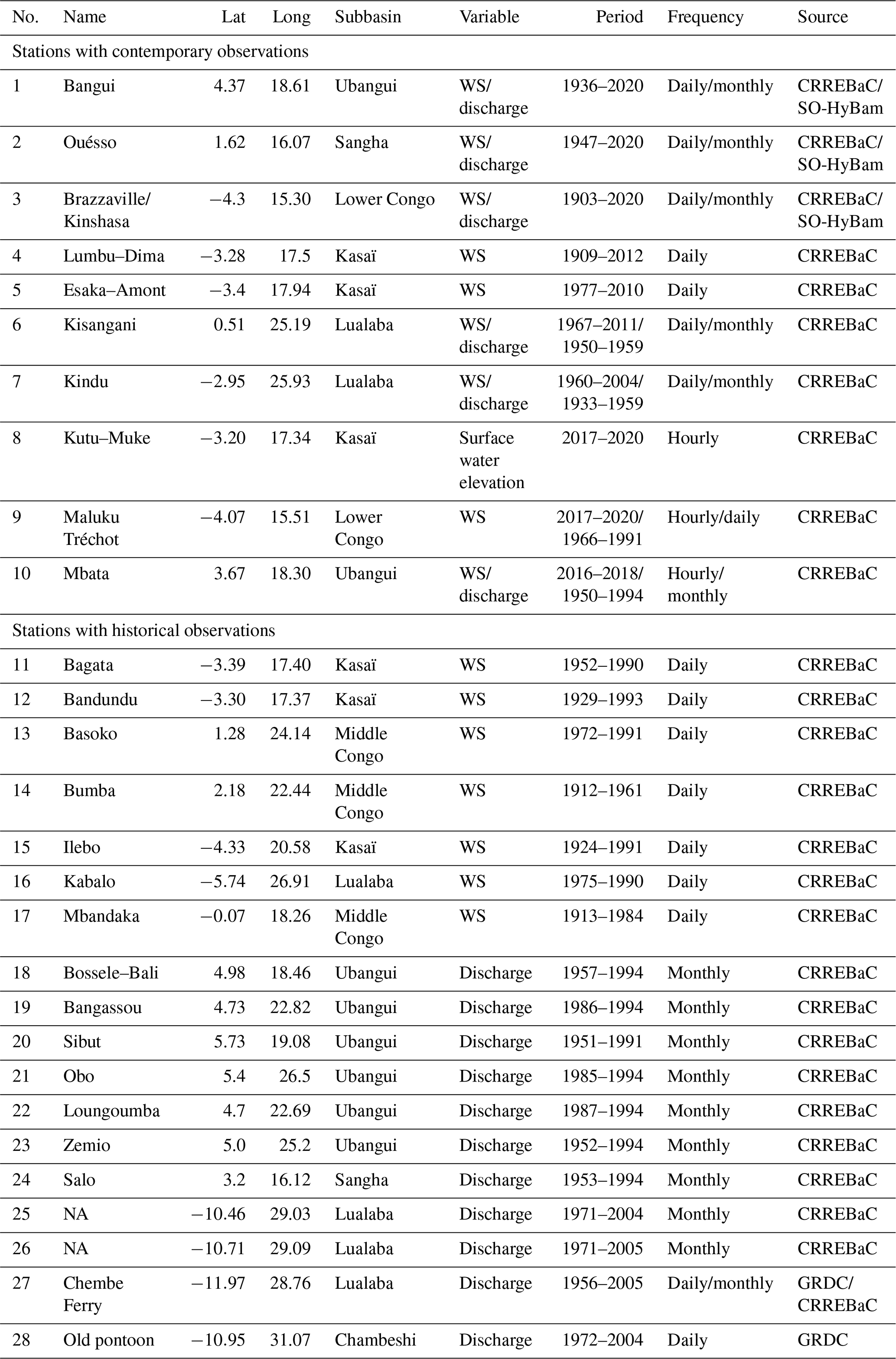
Note: NA stands for not available.
Table 1 is organized in the following two categories: one with stations providing contemporary observations, i.e. covering a period of time that presents a long overlap (several years) with the satellite era (starting in 1995 in our study), and another with stations providing long-term historical observations before the 1990s. In the frame of the Commission Internationale du Bassin du Congo–Ubangui–Sangha (CICOS)/CNES/IRD/AFD spatial hydrology working group, the Maluku Tréchot and Mbata hydrometric stations were set up right under Sentinel-3A (see below) ground tracks. Additionally, for Kutu–Muke, the water stages are referenced to an ellipsoid, which therefore provide surface water elevations.
3.2 Radar-altimetry-derived surface water height
Radar altimeters on board satellites were initially designed to measure the ocean surface topography by providing along-track nadir measurements of water surface elevation (Stammer and Cazenave, 2017). Since the 1990s, radar altimeter observations have also been used for continental hydrology studies and to provide a systematic monitoring of water levels of large rivers, lakes, wetlands, and floodplains (Cretaux et al., 2017).
The intersection of the satellite ground track with a water body defines a virtual station (VS), where surface water height (SWH) can be retrieved with temporal interval sampling provided by the repeat cycle of the orbit (Frappart et al., 2006; Da Silva et al., 2010; Cretaux et al., 2017).
The in-depth assessment and validation of the water levels derived from the satellite altimeter over rivers and inland water bodies were performed over different river basins against in situ gauges (Frappart et al., 2006; Seyler et al., 2008; Da Silva et al., 2010; Papa et al., 2010, 2015; Kao et al., 2019; Kittel et al., 2021; Paris et al., 2022), with satisfactory results and uncertainties ranging between a few centimetres to tens of centimetres, depending on the environments. Therefore, the stages of continental water retrieved from satellite altimetry have been used for many scientific studies and applications, such as the monitoring of abandoned basins (Andriambeloson et al., 2020), the determination of rating curves in poorly gauged basins for river discharge estimation (Paris et al., 2016; Zakharova et al., 2020), the estimation of the spatiotemporal variations in the surface water storage (Papa et al., 2015; Becker et al., 2018), the connectivity between wetlands, floodplains, and rivers (Park, 2020), and the calibration/validation of hydrological (Sun et al., 2012; de Paiva et al., 2013; Corbari et al., 2019) and hydrodynamic (Garambois et al., 2017; Pujol et al., 2020) models.
The satellite altimetry data used in this study were acquired from (1) the European Remote Sensing-2 satellite (ERS-2; providing observations from April 1995 to June 2003 with a 35 d repeat cycle), (2) the Environmental Satellite (ENVISAT, hereafter named ENV; providing observations from March 2002 to June 2012 on the same orbit as ERS-2), (3) Jason-2 and 3 (hereafter named J2 and J3; flying on the same orbit with a 10 d repeat cycle, covering June 2008 to October 2019 for J2 and January 2016 to the present for J3), (4) the Satellite with ARgos and ALtiKa (SARAL/Altika, hereafter named SRL; from which we use observations from February 2013 to July 2016, ensuring the continuity of the ERS-2/ENV long-term records on the orbit, with a 35 d repeat cycle), and (5) Sentinel-3A and Sentinel-3B missions (hereafter named S3A and S3B; available, respectively, since February 2016 and April 2018, with a ∼27 d repeat cycle). While ERS-2, ENV, SRL, and J2 missions are past missions, J3 and S3A/B are still ongoing missions. The VSs used in this study were either directly downloaded from the global operational database of Hydroweb (http://hydroweb.theia-land.fr, last access: 19 January 2022) or processed manually using MAPS and ALTIS software (respectively, Multi-mission Altimetry Processing Software and Altimetric Time Series Software; Frappart et al., 2015a, b, 2021b) and GDRs (geophysical data records) provided freely by the CTOH (Center for Topographic studies of the Oceans and Hydrosphere; http://ctoh.legos.obs-mip.fr/, last access: 19 January 2022). We thus reached a total number of 323 VSs from ERS-2, 364 and 342 VSs for ENV and ENV2 (new orbit of ENVISAT since late 2010), respectively, 146 and 98 VSs for J2 and J3, respectively, 358 VSs for SRL, 354 VSs for S3A, and 326 VSs for S3B (Fig. 2).

Figure 2Locations of altimetry VSs over time within the CRB. (a) ERS-2 VSs, covering the 1995–2002 period. (b) ENV, ENV2, J2, and SRL VSs during 2002–2016. (c) J3, S3A, and S3B VSs from 2016 up to the present. (d) VSs with an actual long time series from a combination of multi-satellite missions, with the record period ranging between 25 and 20 years (yellow), 20 and 15 years (orange), and 15 and 10 years (red).
Figure 2d shows the actual combination of VSs derived from different satellite missions with the purpose of generating long-term water level time series spatialized over the CRB. A total of 25, 20, 14, and 12 years of records were aggregated, respectively, with ERS-2_ENV_SRL_S3A, ERS-2_ENV_SRL, ENV_SRL, and, finally, J2_J3. The pooling of VSs is based on the principle of the nearest neighbour located at a minimum distance of 2 km (Da Silva et al., 2010; Cretaux et al., 2017).
The height of the reflecting water body derived from the processing of the radar echoes is subject to biases. The biases vary with the algorithm used to process the echo, called the retracking algorithm, and with the mission (e.g. orbit errors, onboard system, and mean error in propagation velocity through atmosphere). Therefore, it is required that these biases are removed in order to compose multi-mission series. We used the set of absolute and intermission biases determined at Parintins on the Amazon River, Brazil (Daniel Medeiros Moreira, personal communication, 2020). At Parintins, the orbits of all the past and present altimetry missions (except S3B) have a ground track that is in close vicinity to the gauge. The gauge has been surveyed during many static and cinematic Global Navigation Satellite System (GNSS) campaigns, giving the ellipsoidal height of the gauge as zero and the slope of the water surface. We also took into account the crustal deflection produced by the hydrological load using the rule given by Moreira et al. (2016). Therefore, all the altimetry measurements could be compared rigorously to the absolute reference provided by the gauge readings, making the determination of the biases for each mission and for each retracking algorithm possible. It is worth noting that this methodology does not take into account the possible local or regional phenomena that could have an impact on the biased values. Ideally, similar studies should be carried out at several locations on Earth to verify whether such a regional phenomenon exists or not.
Note that there is no common height reference between altimeter-derived water height (referenced to a geoid model) and the in situ water stage (i.e. the altitude of the zero of the gauges is unknown). Therefore, when we want to compare them, we merge them to the same reference by calculating the difference in the averages over the same period and adding this difference to the in situ water stage.
3.3 Multi-satellite-derived surface water extent
The GIEMS captures the global spatial and temporal dynamics of the extent of episodic and seasonal inundation, wetlands, rivers, lakes, and irrigated agriculture at resolution at the Equator (on an equal-area grid, i.e. each pixel covers 773 km2; Prigent et al., 2007, 2020). It is developed from complementary, multiple satellite observations (Prigent et al., 2007; Papa et al., 2010), and the current data (called GIEMS-2) cover the period from 1992 to 2015 on a monthly basis. For more details on the technique, we refer to Prigent et al. (2007, 2020).
The seasonal and interannual dynamics of the ∼25-year surface water extent have been assessed in different environments against multiple variables, such as the in situ and altimeter-derived water levels in wetlands, lakes, rivers, in situ river discharges, satellite-derived precipitation, or the total water storage from Gravity Recovery and Climate Experiment (GRACE; Prigent et al., 2007, 2020; Papa et al., 2008, 2010, 2013; Decharme et al., 2011). The technique generally underestimates small water bodies comprising less than 10 % of the fractional coverage in equal-area grid cells (i.e. ∼80 km2 in ∼800 km2 pixels; see Fig. 7 of Prigent et al., 2007, for a comparison against high-resolution – 100 m – SAR images; see Hess et al., 2003 and Aires et al., 2013 for details over high and low water seasons in the central Amazon). Note that large freshwater bodies worldwide, such as Lake Baikal, the Great Lakes, and Lake Victoria are masked in GIEMS-2. In the CRB, this is the case for Lake Tanganyika (Prigent et al., 2007). This will impact the total extent of the surface water, but not its relative variations, at basin scale as the extent of Lake Tanganyika itself shows small variations across seasonal and interannual timescales.
4.1 Validation of altimetry-derived surface water height
Observations of in situ WS (see Fig. 1 for their locations; Table 1) over the CRB are compared to radar altimetry SWH (Figs. 3 and 4). The comparisons at nine locations cover five subbasins, including Sangha (Ouésso station; Fig. 3a), Ubangui (Bangui and Mbata stations; Figs. 3d and 4d), Lualaba (Kisangani and Kindu station; Fig. 3j and p), Kasaï (Kutu–Muke and Lumbu–Dima; Fig. 3m and g), and lower Congo (Brazzaville/Kinshasa and Maluku Tréchot stations; Figs. 3s and 4a). In order to evaluate the performance of the different satellite missions, we choose the nearest VSs located in the direct vicinity of the different gauges.
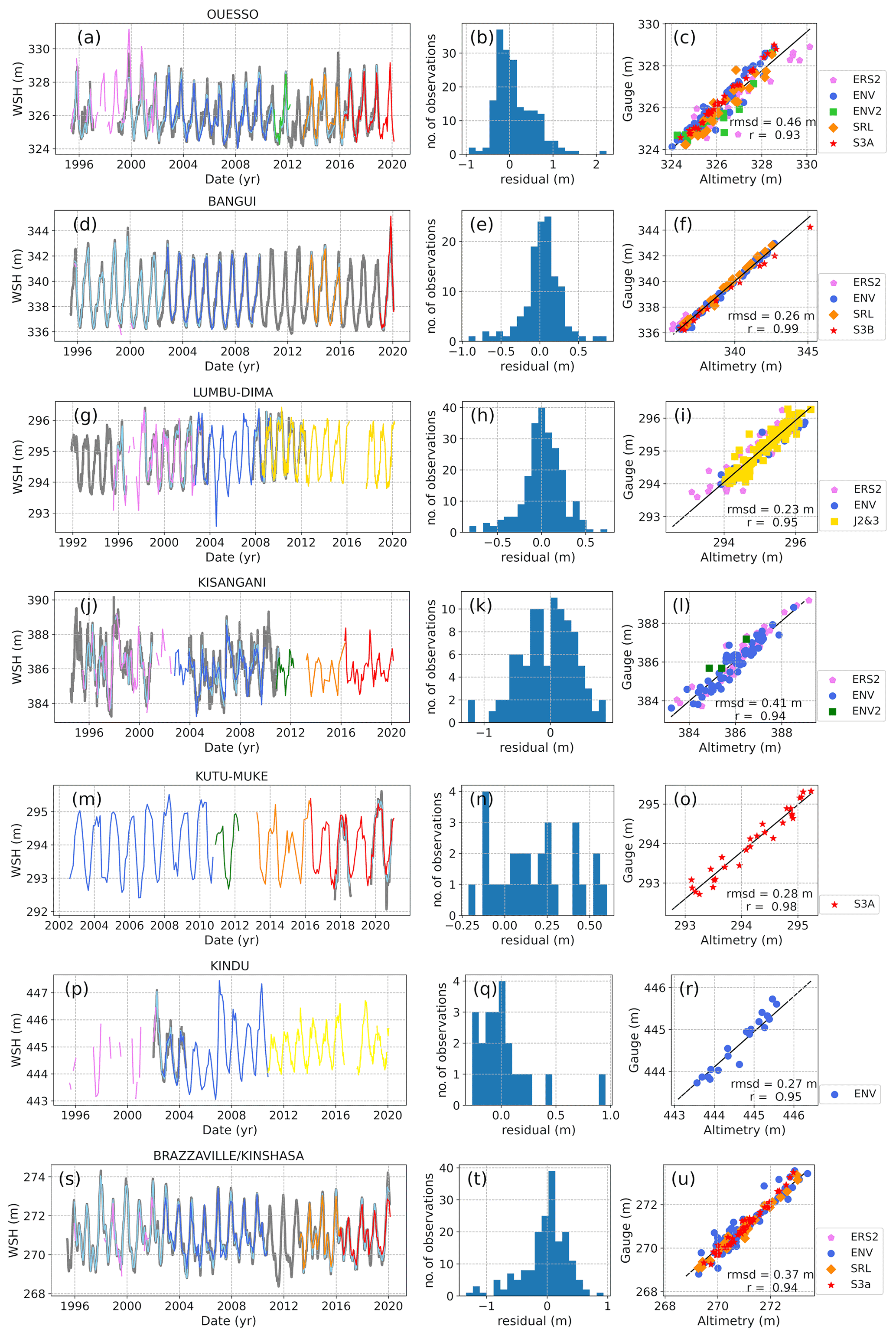
Figure 3Comparison of the in situ water stage (Table 1) and long-term altimeter-derived SWH obtained by combining ERS-2, ENV, ENV2, SRL, J2/3, and S3A/B at different sites (see Fig. 1 for their locations). (a, d, g, j, m, p, s) The time series of both in situ and altimetry-derived water heights, where the grey line in the background shows the in situ daily WS variations (grey), and the sky blue line indicates the in situ WS sampled at the same date as the altimeter-derived SWH from ERS-2 (purple), ENV (royal blue), ENV2 (lime green), SRL (dark orange), J2/3 (yellow), and S3A/S3B (red) missions. (b, e, h, k, n, q, t) The histogram of the difference between the altimeter-derived SWH and the in situ WS. (c, f, i, l, o, r, u) The scatterplot between altimeter-derived SWH and in situ WS. The linear correlation coefficient r and the root mean square deviation (rmsd), considering all the observations, are indicated. The solid line shows the linear regression between both variables.
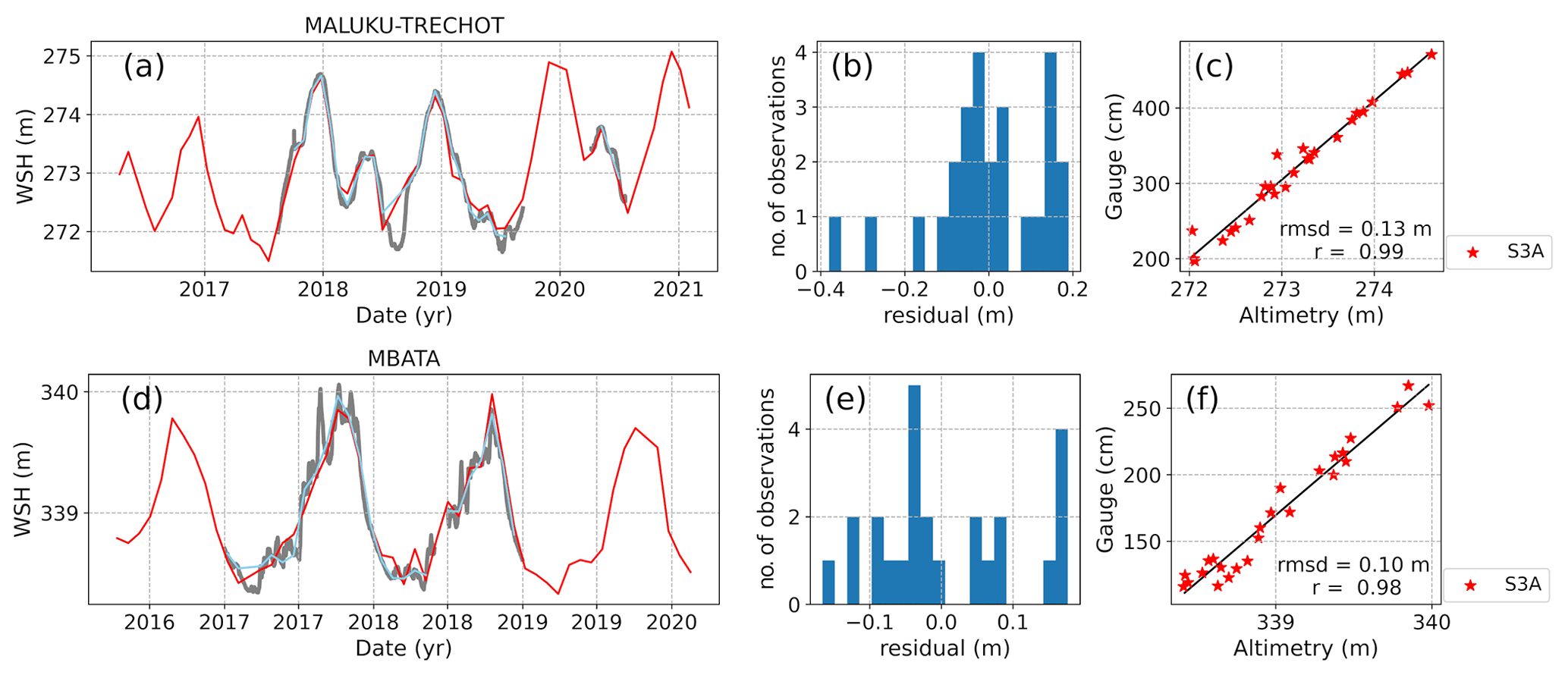
Figure 4Similar to Fig. 3 but the in situ stations are located right below the satellite track of S3A. A comparison of the in situ water stage (Table 1) and S3A altimeter-derived SWH at different sites is shown (see Fig. 1 for their locations). (a, d) The time series of both in situ and altimetry-derived water heights, where the grey line in the background shows the in situ daily WS variations (grey), and the sky blue line indicates the in situ WS sampled at the same date as the altimeter-derived SWH from S3A (red) mission. (b, e) The histogram of the difference between the altimeter-derived SWH and the in situ WS. (c, f) The scatterplot between altimeter-derived SWH and in situ WS. The linear correlation coefficient r and the root mean square deviation (rmsd), considering all the observations, are indicated. The solid line shows the linear regression between both variables.
Figure 3 (left column) provides the first comparison of long-term SWH time series at seven gauging stations. It generally shows a very good agreement, presenting a similar behaviour in the peak-to-peak height variations, within a large set of hydraulic regimes (low- and high-flow seasons). Similar results in the CRB were found by Paris et al. (2022), where the comparisons were done at a seasonal timescale, with a few tens of centimetres of standard error. Note that the VSs of different missions were not located at the same distance from the in situ gauges (distance ranges between 1 and 38 km). The gauge is considered right below the satellite track when its distance is less than 2 km (as in Fig. 4a and d), as reported by Da Silva et al. (2010). This can explain some discrepancies generally observed for the VSs far away from the in situ gauges (distance > 10 km; Fig. 3a). Such discrepancies can be due to severe changes in the cross section between the gauge and the VS, such as changes in river width. For Ouésso (Fig. 3a), ENV2 overestimates the lower water level as compared to the other missions. Figure 3j, m, and p present the benefit of spatial altimetry for completing actual temporal gaps of the in situ observations. Nevertheless, for Kindu (Fig. 3p), ENV and J2 are showing different amplitudes. The difference between radar altimetry water levels and in situ observations (Fig. 3; centre column) shows values of the order of few tens of centimetres (concentration of points around zero in the histograms). The scatterplots between altimetry-derived SWH and in situ water stage presented in Fig. 3 (right column) confirm the good relationship observed in the time series. The correlation coefficient ranges between 0.84 and 0.99, with the average standard error of the overall entire series varying from 0.10 to 0.46 m. The values of root mean square deviation (rmsd) are found to be comparable to others obtained in other basins over the world (Leon et al., 2006; Da Silva et al., 2010; Papa et al., 2012; Kittel et al., 2021). The results obtained from the analysis for each satellite mission at each station are summarized in Table 2.
Table 2The rmsd and r per satellite mission for each in situ station related to Fig. 3.
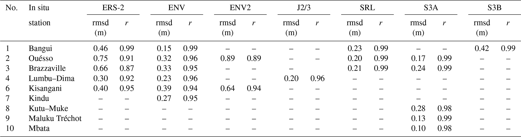
The highest rmsd is 0.75 m at Ouésso station on the Sangha River, related to the ERS-2 mission (Table 2), and the lowest value of rmsd is 0.10 m at Mbata station on the Lobaye River, with S3A mission (Fig. 4d). The pattern observed in Table 2 is that the rmsd decreases continuously from ERS-2 to S3A. In general, ERS-2 presents larger values of rmsd (above 40 cm) than its successor ENV and the lowest coefficient correlation (r) compared to other satellite missions.
These results are in good accordance with Bogning et al. (2018) and Normandin et al. (2018), who observed that the slight decrease in performances of ERS-2 against ENV can be attributed to the lowest chirp bandwidth acquisition mode which degrades the range resolution. The increasing performance with time (from ERS-2 to S3A) is linked to the mode of the acquisition of data from the satellite sensor. ERS-2, ENV, J2/3, and SRL operate in low-resolution mode (LRM) with a large ground footprint, while S3A/B (like other missions such as CryoSat-2) uses the synthetic aperture radar (SAR mode), also known as delay-Doppler altimetry, with a small ground spot (Raney, 1998), resulting in a better spatial resolution than the LRM missions along the track and, thus, a better performance. SRL operating at the Ka band (smaller footprint) and at a higher sampling frequency also shows good performances, as already reported (Bogning et al., 2018; Bonnefond et al., 2018; Normandin et al., 2018). As mentioned above, the accuracy of SWH depends on several factors, among them the width and the morphology of the river. For instance, at the Bangui station on the Ubangui River, S3B surprisingly presents a rmsd of 0.42 m, which is much higher than expected. This can be explained by, amongst others, the fact that its ground track intersects the river in a very oblique way over a large distance (∼3 km) and at a location where the section presents several sandbanks, thus impacting the return signal and resulting in less accurate estimates.
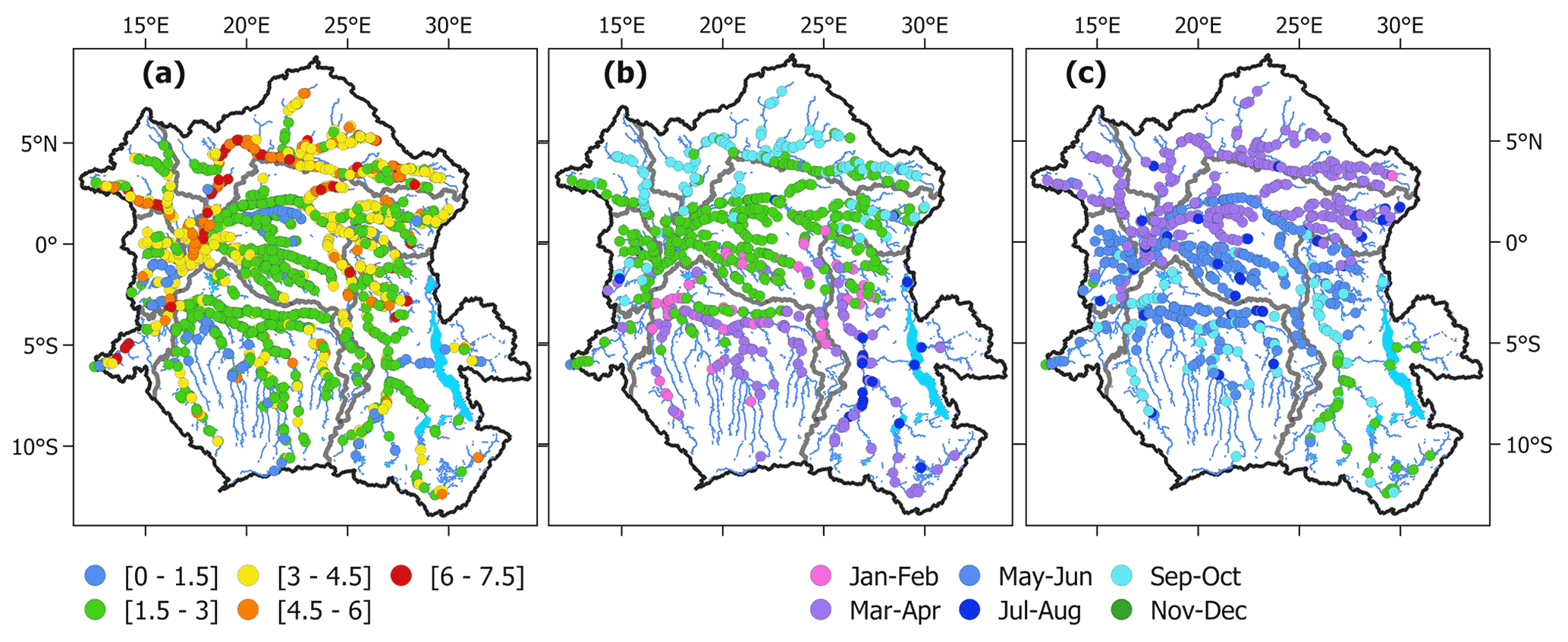
Figure 5Statistics for radar altimetry VSs. (a) The maximum amplitude of SWH (in metres). (b) The average month of the maximum of SWH. (c) The average month of the minimum of SWH.
These validations of radar altimetry SWH in six subbasins of the CRB provide confidence in using the large sets of VSs to characterize the hydrological dynamics of SWH across the basin. Figure 5a provides a representation of the mean maximal amplitude of SWH at each one of those VSs. The Ubangui and Sangha rivers in the northern part of the basin present the largest amplitude variations, up to more than 5 m, while the Congo River main stem and Cuvette Centrale region tributaries vary in smaller proportions (1.5 to 4.5 m). This finding aligns with previous amplitude values reported in the main stem of the Congo River (O'Loughlin et al., 2013). The variation in amplitude in the southern part is similar to the variation observed in the central part, and only a few locations present different behaviours. This is the case, for instance, for the Lukuga river (bringing water from the Tanganyika Lake to the Lualaba river), which is characterized by an amplitude lower than 1.5 m, such as some parts of the Kasaï basin (upper Kasaï, Kwilu, and Wamba rivers) and some tributaries from the Batéké plateaus. The latter are well known for the stability of their flows, due to a strong groundwater regulation.
Figure 5b and c shows the average month for the annual highest and lowest SWH, respectively, at each VS. The high period of water levels in the northern subbasins is September to October, November to December in the central part, and March to April in the southern part. Conversely, the season of low water levels in the northern subbasins is March to April, while the central part of the CRB is at the lowest in May to June, with an exception for the Lulonga river and the right bank tributaries upstream the confluence with the Ubangui (e.g. Aruwimi), for which the driest period is March to April. The Kasaï subbasin is characterized by two periods of low water level, namely September to October and May to June, on the main Kasaï river stem and its other tributaries. Similarly, the major highland Lualaba tributaries (e.g. Ulindi, Lowa, and Elila), fed by the precipitation in the South Kivu region, present lowest levels in May and June. From its confluence with the Lukuga river and up to Kisangani, the Lualaba river reaches its lowest level in September to October. In the Upemba depression, the low SWH period is November–December. This evidences the strong seasonal signal of the gradual floods of the CRB, clearly illustrating the influence of the rainfall partition in the northern and southern parts of the basin and the gradual shifts due to the flood travel time along the rivers and floodplains. This will be further analysed and discussed in Sect. 5.
4.2 Evaluation of surface water extent characteristics from GIEMS-2
Figure 6 shows the surface water extent (SWE) main patterns over the CRB. Figure 6a and b display, respectively, the mean and the mean annual maximum in the extent of surface water over the 1992–2015 period. Figure 6c shows the variability in SWE, expressed in terms of the standard deviation over the period. Figure 6d provides the average month of SWE annual maximum over the record. The figures show plausible spatial distributions of the major drainage systems, rivers, and tributaries (Lualaba, Congo, Ubangui, and Kasaï) of the CRB. The dataset indeed delineates the main wetlands and inundated areas in the region such as in the Cuvette Centrale region, the Bangweulu swamps, and the valley that contains several lakes (Upemba). These regions are generally characterized by a large maximum inundation extent (Fig. 6b) and variability (Fig. 6c), especially in the Cuvette Centrale region and in the Lualaba subbasin, and are dominated by the presence of large lakes and seasonally inundated floodplains. The spatial distribution of GIEMS-2 SWE is in agreement with several other estimates of SWE over the CRB (see Figs. 3 and 6 of Fatras et al., 2021), including L-band SMOS-derived products (SWAF – surface water fraction; Parrens et al., 2017), Global Surface Water extent dataset (GSW; Pekel et al., 2016), the ESA-CCI (European Space Agency Climate Change Initiative) product and SWAMPS (Surface WAter Microwave Product Series) over the 2010–2013 time period. At the basin scale, and in agreement with the results from the altimetry-derived SWH, GIEMS-2 shows that the Cuvette Centrale region is flooded at its maximum in October–November (Fig. 6d), while the Northern Hemisphere part of the basin reaches its maximum in September–October, and the Kasaï and southeastern part reaches its maximum in January–February.
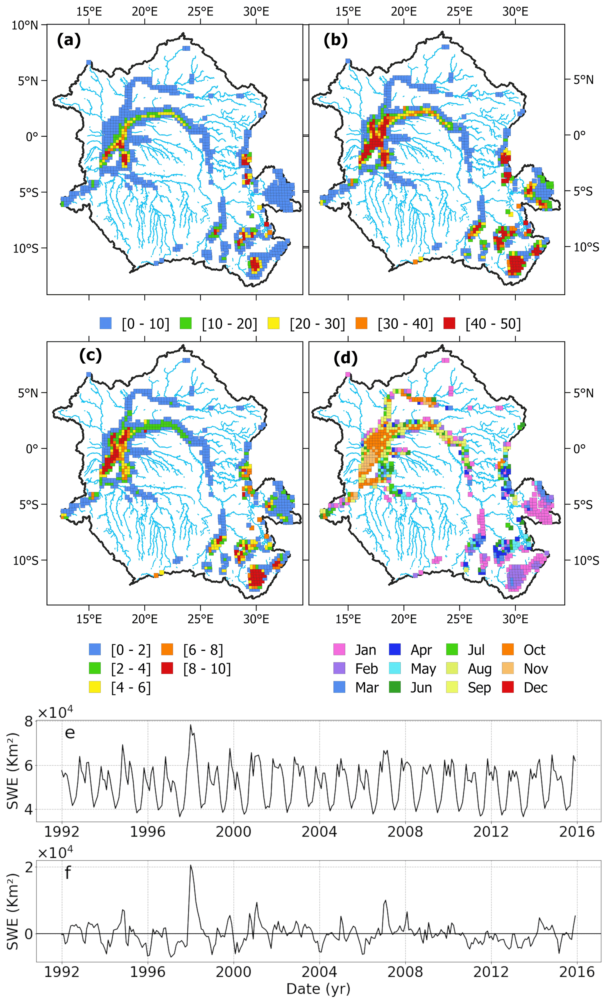
Figure 6Characterization of SWE from GIEMS-2 over the CRB. (a) Mean SWE (1992–2015) for each pixel, expressed as a percentage of the pixel coverage size of 773 km2. (b) SWE variability (standard deviation over 1992–2015; also in percent). (c) Annual maximum SWE averaged over 1992–2015 (in percent). (d) Monthly mean SWE for 1992–2015 for the entire CRB. (e) Time series of SWE. (f) Corresponding deseasonalized anomalies obtained by subtracting the 24 years of mean monthly values from individual months.
Seasonal and interannual variations in the CRB scale total SWE and the associated anomalies over 1992–2015 are shown in Fig. 6e and f. The deseasonalized anomalies are obtained by subtracting the 25-year mean monthly value from each individual month. The total CRB SWE extent shows a strong seasonal cycle (Fig. 6e), with a mean annual averaged maximum of ∼65 000 km2 over the 1992–2015 period, with a maximum ∼80 000 km2 in 1998. The time series shows a bimodal pattern that characterizes the hydrological annual cycle of the CRB. It also displays a substantial interannual variability, especially near the annual maxima. The deseasonalized anomaly in Fig. 6f reveals anomalous events that have recently affected the CRB in terms of flood or drought events. As discussed in Becker et al. (2018), the positive Indian Ocean Dipole (pIOD) events, in conjunction with the El Niño events that happened in 1997–1998 and 2006–2007, triggered floods in east Africa, the western Indian Ocean, and southern India (Mcphaden, 2002; Ummenhofer et al., 2009) and resulted in the large positive peaks observed. The CRB was also impacted by significantly severe and sometimes multi-year droughts during the 1990s and 2000s, often impacting about half of the basin (Ndehedehe et al., 2019). These events can be depicted from GIEMS-2 anomaly time series with repetitive negative signal peaks.
In order to evaluate SWE dynamics at basin and subbasin scales, here we compare at the monthly time step for the seasonal and interannual variability in the GIEMS-2 estimates against the variability in the available in situ water discharge and stages (Table 1).
First, at the entire basin scale, Fig. 7 displays the comparison between the total area of the CRB SWE with the river discharge measured at the Brazzaville/Kinshasa station, which is the most downstream station available for our study near the mouth of the CRB. There is a fair agreement between the interannual variation (Fig. 7a) in the surface water extent and the in situ discharge over the period from 1992 to 2015, with a significant correlation coefficient (r=0.67 with a 0-month lag; p value < 0.01) and a fair correlation for its associated anomaly (r=0.58; p value < 0.01). On both the raw time series and its anomaly (Fig. 7b), SWE captures major hydrological variations, including the yearly and bimodal peaks. The seasonal comparison (Fig. 7c) shows that the SWE reaches its maximum 1 month before the maximum of the discharge in December. From January to March, the discharge decreases, while the SWE remains high. For the secondary peak, the SWE maximum is reached 2 months before the one for discharge in May. This is in agreement with the results shown with the SWE spatial distribution of the average month of the maximum inundation in October–November in the Cuvette Centrale region (Fig. 6a).
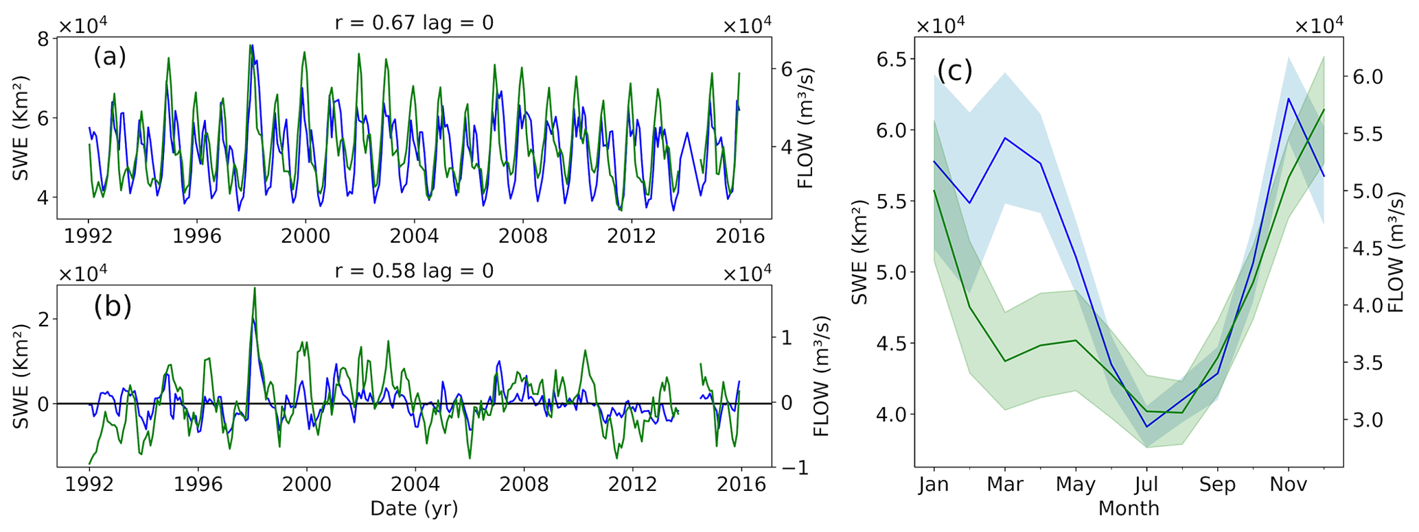
Figure 7Comparison of monthly SWE (a) and its anomalies (b) at CRB scale against the in situ monthly mean water discharge at the Brazzaville/Kinshasa station. The blue line is the SWE, and the green line is the mean water discharge. (c) The annual cycle for both variables (1992–2015), with the shaded areas illustrating the standard deviations around the SWE and discharge means.
Further, the evaluation of SWE dynamics is performed at the subbasin level against available observations at the outlets of each of the 5 subbasins. Similar to Fig. 7, Fig. 8 shows the comparisons of the aggregated SWE at the subbasin scale against in situ observations at their respective outlet stations (Bangui for Ubangui, Ouésso for Sangha, Lumbu–Dima for Kasaï, Kisangani for Lualaba, and Brazzaville/Kinshasa for the middle Congo subbasin). For Lualaba and Kasaï (Fig. 9), in situ SWHs are used since no discharge observation is available. For each subbasin, we estimate the maximum linear correlation coefficient of point time records between the SWE and the other variables when lagged in time (months). The temporal shift helps to express an estimated travel time of water to reach the basin outlet. There is a general good agreement (with high lagged correlations r>0.8; Figs. 8a, d, g and 9a) between both variables, and lag time ranging between 0 and 2 months, with SWE preceding the discharge, except for the Lualaba. The seasonal analysis in Ubangui and Sangha subbasins shows that the discharge starts to increase one month prior to SWE (from May), probably related to local precipitation downstream the basins, before both variables increase steadily and reach their maximum in October–November (Fig. 8c and f). For the Kasaï subbasin (Fig. 9c), SWE increases from July, followed within a month by the water stage, reaching a peak respectively in December and January. While SWE slowly decreases from January, only the discharge continues to increase to reach a maximum in April. For the middle Congo subbasin (Fig. 8), the variability in SWE and discharge are in good agreement (r=0.89, Fig. 8g) with the SWE steadily preceding the discharge by one month (Fig. 8i). The annual dual peak is also well depicted. On the other hand, the Lualaba subbasin with a moderate correlation (r=0.54 and lag = 0 month; Fig. 9d) shows a particular behaviour with the water stage often preceding the SWE (Fig. 9f). This could be explained by the upstream part of the Lualaba subbasin where the hydrology might be disconnected from the drainage system due to the large seasonal floodplains and lakes, well captured by GIEMS. These water bodies store freshwater and delay its travel time, while the outlet still receives water from other tributaries in the basin. For all subbasins, the inter-annual deseasonalized anomalies present in general positive and moderate linear correlations (; p value < 0.01 with 0-month lag; Figs. 8b, e and 9b, e) except for the middle Congo where the correlation is greater (0.63; p value < 0.01) with temporal shift of one month (Fig. 8h). This confirms the good capabilities of satellite-derived SWE to portray anomalous hydrological events in agreement with in situ observations at the subbasin scale.
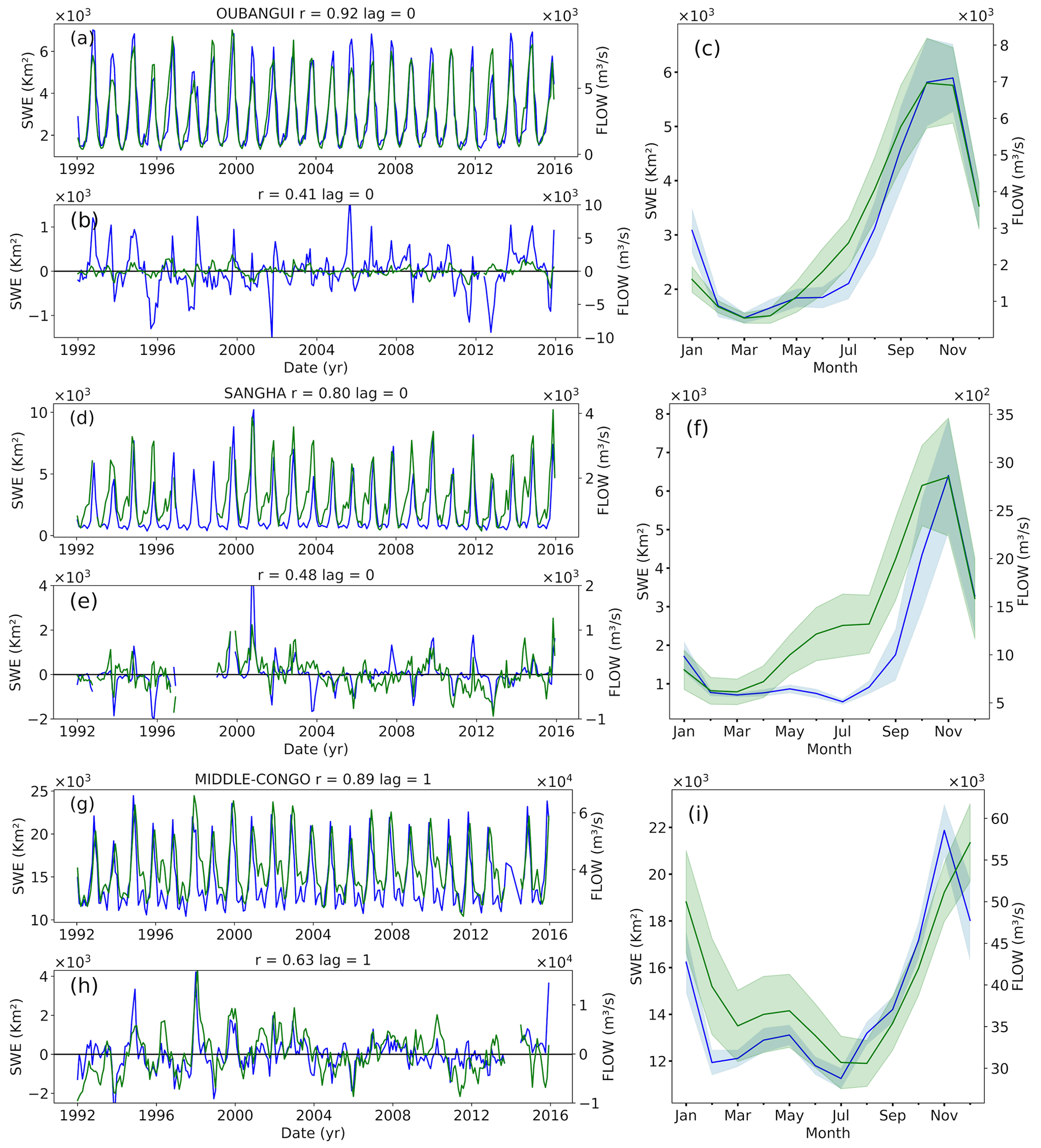
Figure 8Similar to Fig. 7 but for each of the five subbasins. A comparison of the monthly SWE (absolute and anomaly values) against the in situ water discharge at each subbasin outlet is shown. The blue line is for the SWE, and the green line is for the water discharge. The annual cycle for both variables (1992–2015) is also displayed, with the shaded areas illustrating the standard deviations around SWE and discharge means.

Figure 9Similar to Fig. 8 using available in situ water stage. A comparison of the monthly SWE (absolute and anomaly values) against the in situ water stage at each subbasin outlet is shown. The blue line is for the SWE, and the green line is for the water stage. The annual cycle for both variables (1992–2015) is also displayed, with the shaded areas illustrating the standard deviations around SWE and discharge means.
At the basin scale, we have already showed that the annual variability in the CRB discharge is in fair agreement with the dynamic of SWE, from seasonal to interannual timescales. Figure 10 investigates the comparison between water flow at the Brazzaville/Kinshasa station against the variability in SWE for each subbasin. For Ubangui, Sangha, and middle Congo (Fig. 10a, d and g), the variability in water discharge is strongly related to the SWE variations with a respective lag of 2, 1, and 0 months, related to the decreasing distance between the subbasin and the gauging station. The time series of the anomalies of the above subbasins capture also some of the large peak variations while other peaks are observed at the subbasin scale. Kasaï subbasin presents a good correspondence (r=0.74 and lag = 0) between the variability in water flow and SWE, as well as for their associated anomaly (r=0.47 and lag = 0). Unlike the other four sub-catchments, Lualaba presents again a low agreement (r=0.05 and lag = 0) with, as already seen in Fig. 9, a non-consistent behaviour and shifted variations between SWE and discharge (Fig. 10m), related to lakes and floodplains storage which delay the water transfer to the main river. Nevertheless, anomalies like the strong one in 1998, with large floods linked to a positive Indian Ocean Dipole in conjunction with an El Niño (Becker et al., 2018) are in phase and within same order of magnitude (Fig. 10n).
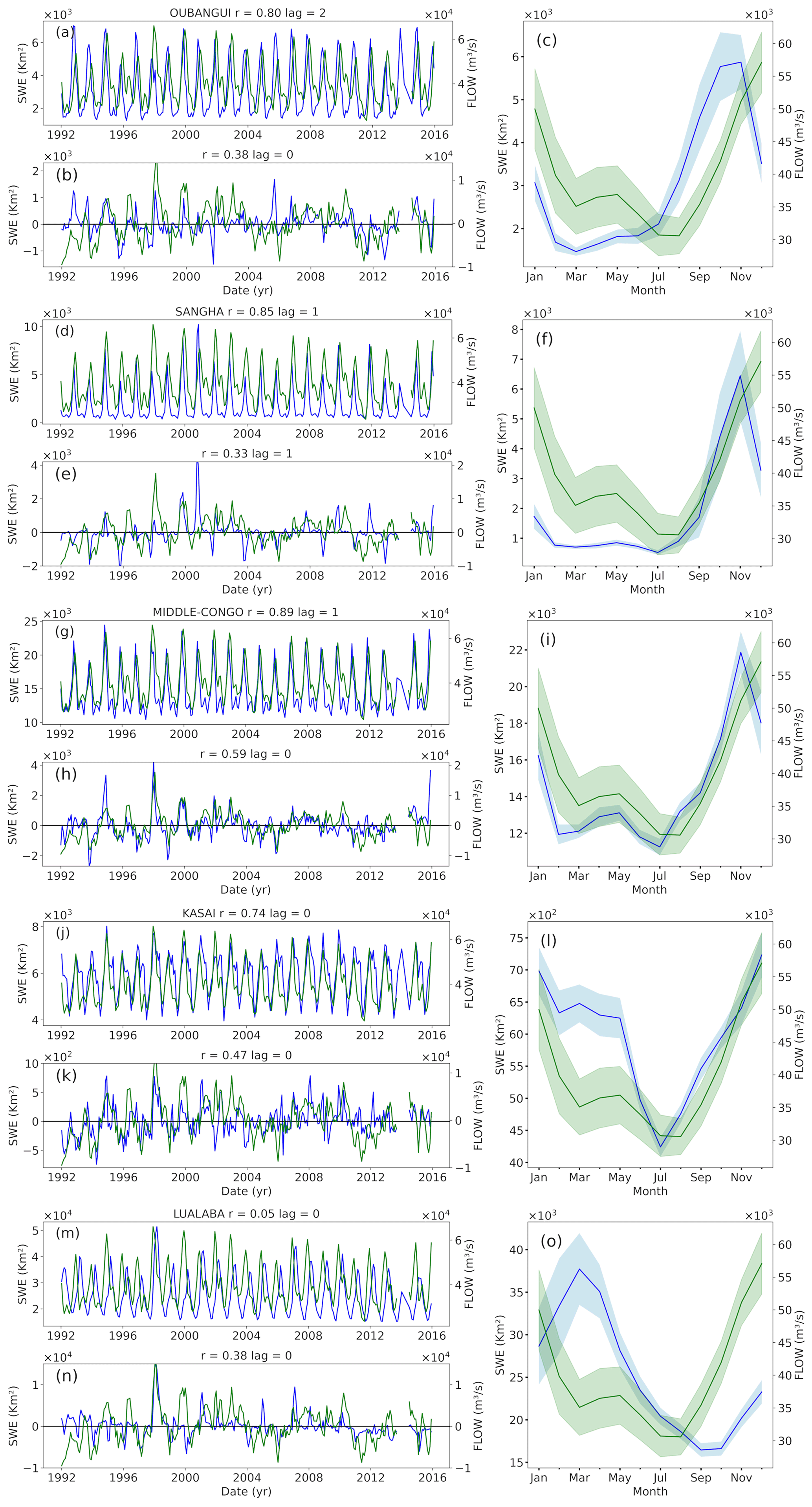
Figure 10Similar to Figs. 7–9 but the SWE estimated at each of the five subbasins is compared against the in situ monthly mean water discharge at the Brazzaville/Kinshasa station. The blue line is for the SWE, and the green line is for the water flow at the Brazzaville/Kinshasa station. The annual cycle for each variable (1992–2015) is also displayed, with the shaded areas illustrating the standard deviations around the SWE and discharge means.
A focus on the middle Congo anomaly time series reveals that it is the only subbasin where all the variations in the peak discharge are well captured in SWE. This reflects the strong influence of the middle Congo floodplains on the flow at the Brazzaville/Kinshasa station, for which the variability may be explained, at ∼35 %, by the variations in SWE in the Cuvette Centrale region, based on the maximum lagged correlation of 0.59 for the deseasonalized anomalies of the two variables. More interestingly, while the river discharge shows a double peak in its seasonal climatology (a maximum peak in December and a secondary peak in May), it is not portrayed in the SWE in most subbasins, except for the middle Congo that also receives contributions from Sangha, Ubangui, Kasaï, and Lualaba. The next section investigates these characteristics.
The evaluation of both SWH from radar altimetry and SWE from GIEMS-2, presented in the previous sections, provides the confidence to further analyse the dynamics of surface water and their patterns within the CRB.
5.1 Seasonal water travel time through the rivers and subbasins of the CRB
The water travel time through the rivers and subbasins of the CRB was previously investigated by using observations from a few in situ gauges (Bricquet, 1993). In this study, SWH and SWE datasets enable a similar analysis at the large scale, with an extended analysis to the entire CRB.
Here, we determine the maximum of the linear Pearson correlation coefficient by considering a time lag between the satellite-derived SWH at each VS (from ERS-2, ENV, J2/3, SRL, and S3A missions) and GIEMS SWE at each cell, against the Brazzaville/Kinshasa SWH and discharge, respectively. For this, we use the scipy.stats.pearsonr package from Python that also includes the computation of the p value that we use for performing the hypothesis test of the significance of the correlation coefficient. In the following, we consider the significance level to be 0.1.
Note that the temporal shift between SWH/SWE and in situ stages and discharges is constrained between acceptable values, i.e. it cannot be negative, as we are investigating the time needed by surface waters to reach the Brazzaville/Kinshasa station. For each VS, the longest possible time series is used. For GIEMS-2, the data over the 24-year record are used against the entire river discharge record (1992–2015). The maps of the highest correlations and their corresponding time shifts are provided in Fig. 11. Note that both satellite-derived datasets are jointly analysed to support and complement each other's individual result. As a validation, the linear Pearson correlation coefficients between altimeter-derived SWH and GIEMS-2 SWE for each location within a 25 km distance and a common availability of data were estimated (figure not shown). The correlations found are generally high (>0.9) across the entire CRB.

Figure 11Maps of the optimal coefficient correlation and associated lag at each VS and GIEMS-2 cell. (a) Optimum coefficient correlation between altimetry-derived SWH (from ERS2, ENV, SRL, J2/3, and S3A missions) at each VS against the in situ water stage at the Brazzaville/Kinshasa station. (b) Same as (a) for each GIEMS-2 cell against the river discharge at the Brazzaville/Kinshasa station. Panels (c) and (d) show, respectively, their optimum lag in months. In panels (c) and (d), only the time lags for which the maximum correlation has a p value < 0.05 are displayed.
Figure 11a and b evidences that the northern (Sangha and Ubangui) and the central (western middle Congo and downstream tributaries of Kasaï) parts are fairly well correlated (r>0.6; p value < 0.1), both in terms of SWH and SWE to the discharge at Brazzaville/Kinshasa. In the eastern part of the middle Congo and downstream part of the Lualaba river, SWH and SWE show different patterns, with higher maximal correlations for SWH (>0.6) than SWE (<0.5). On the other hand, the southeastern part of the Lualaba subbasin presents a low correlation (r<0.2) for both variables, confirming again that the discharge at the Brazzaville/Kinshasa station is not strongly influenced by the remote water dynamics from the southeastern part of the CRB. The temporal shifts (in months) associated to the maximum correlation (Fig. 11c and d) at each VS and GIEMS-2 cell (only locations where r≥0.6 are displayed) help to estimate the water travel time to the Brazzaville/Kinshasa reach. As expected, the time lag for both SWH and SWE increases with the distance from the Brazzaville/Kinshasa station from 0 up to 3 months in remote areas and small tributaries of the upper CRB. The mainstream of the Congo in the middle Congo subbasin and northern Kasaï are characterized by 0 months of lag due to their proximity with the reference station (Brazzaville/Kinshasa). However, left- and right-margin tributaries (for instance, the Likouala-aux-Herbes and Ngoko rivers) present a 1-month lag. The Ubangui and Sangha subbasins show a minimum of 2 months' lag and up to 3 months for the remote area in the far northern part of the Ubangui basin (Kotto and Mbomou rivers; Fig. 11c). Interestingly, on the downstream part of the Ubangui river, and in the Cuvette Centrale region, there is a notable 1-month difference between the lag in SWH and SWE. While SWH shows a lag time of 0–1 month, it is 1–2 months for SWE. This can be explained by specific hydrological mechanisms of wetlands and large floodplains and the processes between river and floodplains connectivity. These differences can be due, on the one hand, to the different behaviours between the water level dynamics and water extent in shallow flooded areas, where SWH in river generally increases before the surface water extent increases with riverbank overflows, while the waters stand for a longer time in the wetlands than in the rivers. The differences might also be attributed to relatively disconnected wetlands and rivers and/or to the presence of interfluvial wetlands fed directly by local precipitation instead of overbank flooding.
In order to confirm and validate the results on the dynamics of water surface flows obtained from altimeter-derived SWH and GIEMS-derived SWE, we perform a similar analysis using water level and flow observations from historical (<1994) and current gauges, as presented in Table 2. For each station, covering all the subbasins considered, we estimated the correlation between the available observations and the observations at the Brazzaville/Kinshasa station at daily and monthly time steps. The results are presented in Table 3. In order to facilitate the comparisons, results for the VSs and SWE cells (as presented in Fig. 11) related to the nearest available in situ gauge stations are reported in Table 3, even if not covering the same period of time.
Table 3Optimal coefficient correlation and associated lag for each in situ station against SWH and discharge at the Brazzaville/Kinshasa station, with their closest VS and GIEMS-2 cell (SWE) and their latitude and longitude in parentheses (second column). In the last two columns, in parenthesis, the r and lag values are given at the daily timescale when daily observations are available. Only correlations with a 95 % significance are reported.
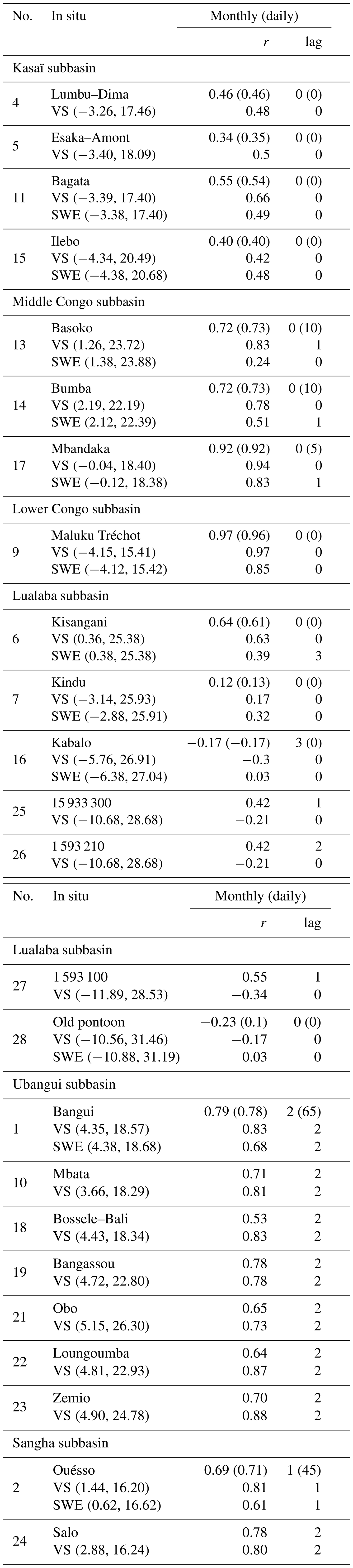
Overall, the results from the Table 3 support the general findings reported in Fig. 11, both in terms of optimum coefficient correlation and in terms of lag, with a general good agreement between in situ and satellite observations. The correlation analysis (with p value < 0.05; the change in the p value is related to the in situ record length) between observations at Brazzaville/Kinshasa and the various other stations confirms the higher positive values (r>0.7; with a mean time lag of 8 d and 0 months) with increasing maximum correlation when closest to Brazzaville/Kinshasa in situ station. Lower Congo also shows very high correlations (r>0.8). The Kasaï subbasin presents low to moderate positive lagged correlation (0.35 to 0.55; lag = 0), with values decreasing with respect to longer distance from the month, which is in agreement with the results from the satellite estimates. For the Lualaba subbasin, the results at the Kisangani outlet station present a moderate maximum correlation (r>0.6), similar to the values obtained with SWH from altimetry. In agreement with the results for both SWH and SWE, in situ observations confirm that, in other upstream locations of the Lualaba, which are connected to lakes and floodplains, very low correlations (r<0.2) are observed. Both Ubangui and Sangha subbasins have large positive correlations (r>0.7), with a respective time lag of 2 months (65 d when using in situ daily observations) and 1 month (45 d), similar to what satellite observations provided. The difference observed in the correlation coefficient and the lag between SWH and SWE, for the Basoko station in middle Congo, for instance, also confirms the different hydrological behaviour between the adjacent wetlands and the main river channel. This is also in line with the 1-month lag observed at some locations in the Cuvette Centrale region between both satellite-derived SWH and SWE, supporting the idea that different processes drive the relation between river channel height and flood extent dynamics.
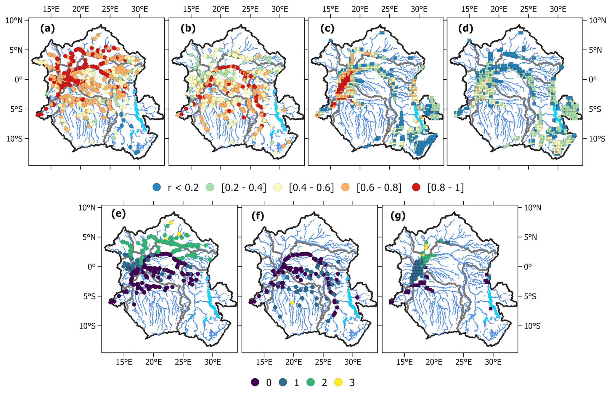
Figure 12Similar to Fig. 11 but considering the two distinct periods of the year corresponding to each hydrological peak observed at Brazzaville/Kinshasa. (a) The optimum coefficient correlation between altimetry-derived SWH (from ERS2, ENV, SRL, J2/3, and S3A missions) at each VS against the in situ water stage at the Brazzaville/Kinshasa station for the period of August–February. (b) Same as panel (a) but for the period of March–July. (c) The optimum coefficient correlation between SWE at each GIEMS-2 against in situ discharge at the Brazzaville/Kinshasa station for the period of August–February. (d) Same as panel (c) but for the period of March–July. (e–g) The time lag (in months) associated, respectively, to panels (a–c) but only for cases where the maximum correlation has p value < 0.05. The time lag associated to panel (d) has too few values with a p value < 0.05 and is therefore not shown.
5.2 Subbasin contributions to the CRB bimodal hydrological regime
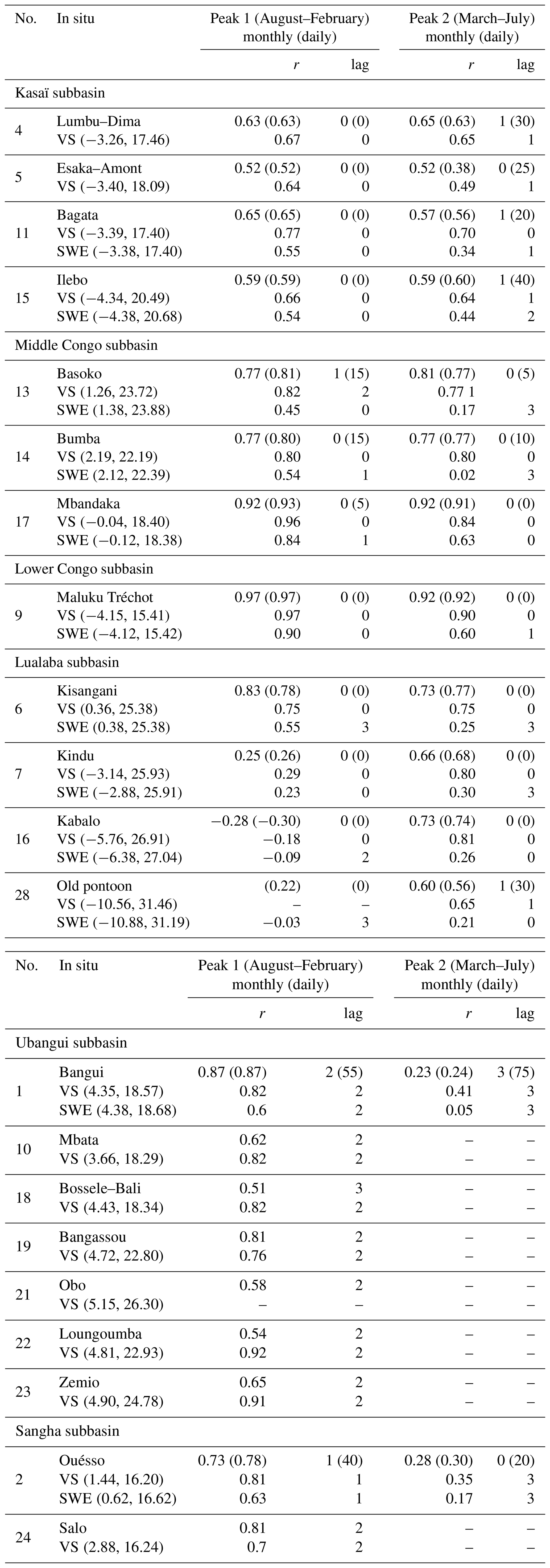
A supplementary analysis was performed in order to better illustrate the spatial distribution of the CRB flood dynamics over all the various tributaries and also their different timing and how each subbasin contributes to the peculiar bimodal pattern of the hydrological regime downstream the main stem at Brazzaville/Kinshasa (Figs. 11 and 12). Here, we reproduced the same analysis as above but now considering, individually, the two distinct periods of the year corresponding to each hydrological peak observed at Brazzaville/Kinshasa. We first consider the August–February period (the first large peak) for each time series and estimate the correlation. Then we consider the March–July period corresponding to the secondary peak. The results are shown in Fig. 12, and the comparison/validation of the results with historical and current in situ records are summarized in Table 4.
Figure 12 clearly depicts the relative contributions of the northern subbasins and the southern subbasins to the first peak and to the second peak, respectively. Regarding the first peak (Fig. 12a, c, e, and g), the major contribution of the Ubangui and Sangha rivers (r>0.6) to the downstream main stem at Brazzaville/Kinshasa during the August–February period is evidenced, with a water transfer time to the Brazzaville/Kinshasa station ranging between 1 and 3 months (again, increasing with the distance to the gauging station). Middle Congo, northern Kasaï, and the highland of the Lualaba subbasin also show some contribution during this period but with 0 to 1 month lag. Water that supplies the second peak of the hydrograph essentially comes from the centre and the southern part of the basin (Fig. 12b, d, and f), including remote rivers in the Kasaï subbasin with a 1–2 month lag and the western part of the Lualaba. The very low correlations between the upper part of the basin (Kivu region, Luapula, and upper Lualaba) and the discharge at Brazzaville/Kinshasa suggest that the contribution in terms of discharge of this region to the hydrological cycle downstream is negligible, for both peaks, in comparison to that from other tributaries. These conclusions are supported by the similar analyses performed using the in situ observation records (Table 4). This confirms the relatively low contribution of the northern part to the second peak at the Brazzaville/Kinshasa station. On the monthly basis, the lags are found to be similar to the in situ and satellite observations, while the daily data from the in situ records help to provide a better characteristic of the travel time at a finer timescale. For instance, with the second peak of the hydrograph, the Kasaï and middle Congo subbasins are characterized, respectively, by a mean time lag of 1 month (28 d) and 0 months (7 d), depending on the data sampling interval considered.
Table 4Optimal coefficient correlation and associated lag for each in situ station against SWH and discharge at the Brazzaville/Kinshasa station for the two periods of time corresponding to the first and second peak and for their closest VS and GIEMS-2 cell (SWE). Their latitude and longitude are in parentheses in the second column. In parenthesis, in the last two columns, the r and lag values, using daily observations are shown. Only correlations with a 95 % significance are reported.
The present study uses a unique joint analysis of in situ and satellite-derived observations to better characterize the CRB surface hydrology and its variability. First, thanks to the availability of an in situ database of historical and contemporary observations of water levels and discharges, we provide an intensive and comprehensive validation of long-term (∼25-year) time series from space-borne water level variations and surface water extent throughout the CRB. The comparison of radar-altimetry-derived water levels with the in situ water stage at the interannual scale shows an overall good agreement, with standard errors, in general, lower than 0.30 m. The analysis of the rmsd across the various missions shows an improvement over time from ERS-2 (tens of centimetres) to S3A/B (a few centimetres) missions, confirming the technological improvement in terms of sensors and data processing. A total of more than 2300 VSs covering the 1995–2020 period was used in this study and is now freely available. When compared to in situ observations, GIEMS-2 SWE also shows consistent and complementary information at the subbasin and basin scales. These two long-term records are then used to analyse the spatiotemporal dynamics of surface freshwater and its propagation at subbasin and basin scales, significantly improving our understanding of how surface water flows in the CRB.
The analysis of the large database of SWH from altimetry shows that the amplitude varies greatly across the basin, from more than 5 m in the Ubangui and Sangha rivers, while the Cuvette Centrale region and the southern basins display smaller annual variations (1.5 to 4.5 m). The maximum level is reached in September–October in the northern part of the basin, in November–December in the central part, and in March–April in the Lualaba region. Surface water bodies and wetlands in the Lualaba subbasin and Cuvette Centrale region present the highest variation in extent across the subbasins and reach their maximum inundation, respectively, in January–February and November–December. Then we investigate the hydrology contributions and water travel times from upstream to downstream reaches by comparing SWE and SWH to stage and discharge at the Brazzaville/Kinshasa station. In particular, the methodology permitted us to better illustrate the spatial distribution of the CRB flood dynamics on the various tributaries, their different timing, and how each subbasin contributes to the peculiar bimodal pattern of the hydrological regime downstream of the main stem in Brazzaville/Kinshasa. The time shift for both SWH and SWE increases with the distance from the Brazzaville/Kinshasa station from no time lag at the vicinity of the outlet up to 3 months in remote areas and small tributaries of the CRB. Northern subbasins and the central Congo region highly contribute to the large August–March peak, while the southern part supplies water to both peaks and in particular to the second one. These results are supported by in situ observations to confirm the findings from satellite observations and from previous studies. Our results therefore confirm the suitability of both long-term water surface elevation time series from radar altimetry and flooded areas from GIEMS-2 for monitoring the CRB surface water dynamics, potentially bridging the gap between past in situ databases and current and future monitoring as an ensemble. Their use in hydrological models will permit a better representation of local- and basin-scale hydrodynamics and ensure an improved monitoring of hydrological variables from space.
The very first use of a large dataset of VSs spread over more than 100 tributaries across the basin and spanning the whole altimetry period permitted an unprecedented analysis in terms of both the length of the observation and number of observations, providing time series of more than 20 years over the CRB. This unique dataset of surface water levels variations, combined to the ∼25-year SWE from GIEMS, should permit us to generate estimates of surface water storage. Complementary to the GRACE/GRACE-FO (Gravity Recovery and Climate Experiment Follow-On) total water storage estimates, it will further permit the estimation of long-term and interannual variations in the freshwater volume in the CRB, including subsurface and groundwater storage and their link with hydro-climatic processes across the region. Furthermore, the use of both satellite datasets in the hydrological models will permit a better representation of local- and basin-scale hydrodynamics and ensure an improved real-time monitoring of hydrological variables from space, as well as a better evaluation of climate variability impacts on water availability. These datasets will also play a key role in the evaluation and validation of future hydrology-oriented satellite missions, such as the NASA-CNES Surface Water and Ocean Topography (SWOT), which is to be launched in late 2022. More generally, the use of satellite-derived observations dedicated to surface hydrology will contribute to a better fundamental understanding of the CRB and its hydro-climatic processes, bringing more opportunities for other river basins in Africa to improve the management of water resources.
Finally, the better understanding of large-scale CRB surface hydrology variability will help to improve the comprehension at the local and regional scales of the hydrological and biogeochemical cycles, as the CRB is recognized to be one of the three main convective centres in the tropics, and its inland waters strongly contribute to the carbon cycle of the basin. Our findings also highlight the large spatiotemporal variability in the surface hydrologic components within the basin that will help understand the links and feedback with regional climate and the influence of events such as El Niño–Southern Oscillation (ENSO) on water resources. The results from both long-term SWH from radar altimetry and flooded areas from GIEMS-2 have confirmed the benefits of Earth observation in characterizing and understanding the variability in the surface hydrologic components in a sparsely gauged basin such as the CRB. Since these datasets are global, our study and the methodology will benefit similar investigations in other ungauged tropical river basins.
The altimetry data over inland water bodies are distributed via the Hydroweb website (time series of water levels in the rivers and lakes around the world, http://hydroweb.theia-land.fr/; Hydroweb, 2022). The SWH dataset over the Congo is freely available from this online platform. For GIEMS-2, the dataset is available upon request to Catherine Prigent (catherine.prigent@obspm.fr).
BK, FP, AP, RTM, and SC conceived the study. BK processed the data and performed the analysis. BK, FP, and AP analysed and interpreted the results and wrote the draft. RTM and CP were responsible for the data curation. All authors discussed the results and contributed to the final version of the paper.
The contact author has declared that neither they nor their co-authors have any competing interests.
Publisher's note: Copernicus Publications remains neutral with regard to jurisdictional claims in published maps and institutional affiliations.
Benjamin Kitambo has been supported by a doctoral grant from the French Space Agency (CNES), Agence Française du Développement (AFD), and Institut de Recherche pour le Développement (IRD). This research has been supported by the CNES TOSCA project “DYnamique hydrologique du BAssin du CoNGO (DYBANGO)” (2020–2023).
This research has been supported by the Centre National d'Etudes Spatiales (project TOSCA DYBANGO).
This paper was edited by Shraddhanand Shukla and reviewed by Paul Bates and one anonymous referee.
Aires, F., Papa, F., and Prigent, C.: Along-term, high-resolution wetland dataset over the Amazon basin, downscaled from a multiwavelength retrieval using SAR data, J. Hydrometeorol., 14, 594–607, https://doi.org/10.1175/JHM-D-12-093.1, 2013.
Aloysius, N. and Saiers, J.: Simulated hydrologic response to projected changes in precipitation and temperature in the Congo River basin, Hydrol. Earth Syst. Sci., 21, 4115–4130, https://doi.org/10.5194/hess-21-4115-2017, 2017.
Alsdorf, D., Beighley, E., Laraque, A., Lee, H., Tshimanga, R., O'Loughlin, F., Mahé, G., Dinga, B., Moukandi, G., and Spencer, R. G. M.: Opportunities for hydrologic research in the Congo Basin, Rev. Geophys., 54, 378–409, https://doi.org/10.1002/2016RG000517, 2016.
Andriambeloson, J. A., Paris, A., Calmant, S., and Rakotondraompiana, S.: Re-initiating depth-discharge monitoring in small-sized ungauged watersheds by combining remote sensing and hydrological modelling: a case study in Madagascar, Hydrolog. Sci. J., 65, 2709-2728, https://doi.org/10.1080/02626667.2020.1833013, 2020.
Becker, M., Santos, J., Calmant, S., Robinet, V., Linguet, L., and Seyler, F.: Water Level Fluctuations in the Congo Basin Derived from ENVISAT Satellite Altimetry, Remote Sens., 6, 9340–9358, https://doi.org/10.3390/rs6109340, 2014.
Becker, M., Papa, F., Frappart, F., Alsdorf, D., Calmant, S., da Silva, J. S., Prigent, C., and Seyler, F.: Satellite-based estimates of surface water dynamics in the Congo River Basin, Int. J. Appl. Earth Obs. Geoinf., 66, 196–209, https://doi.org/10.1016/j.jag.2017.11.015, 2018.
Bele, Y., Mulotwa, E., Bokoto de Semboli, B., Sonwa, D., and Tiani, A.: Afrique centrale: Les effets du changement climatique dans le Bassin du Congo: la nécessité de soutenir les capacités adaptatives locales, CRDI/CIFOR, Canada, 5 pp., https://idl-bnc-idrc.dspacedirect.org/bitstream/handle/10625/45639/132108.pdf (last access; 6 April 2022), 2010.
Betbeder, J., Gond, V., Frappart, F., Baghdadi, N. N., Briant, G., and Bartholomé, E.: Mapping of Central Africa forested wetlands using remote sensing, IEEE J. Select. Top. Appl. Earth Obs. Remote Sens., 7, 531–542, https://doi.org/10.1109/JSTARS.2013.2269733, 2014.
Bogning, S., Frappart, F., Blarel, F., Niño, F., Mahé, G., Bricquet, J. P., Seyler, F., Onguéné, R., Etamé, J., Paiz, M. C., and Braun, J. J.: Monitoring water levels and discharges using radar altimetry in an ungauged river basin: The case of the Ogooué, Remote Sens., 10, 350, https://doi.org/10.3390/rs10020350, 2018.
Bonnefond, P., Verron, J., Aublanc, J., Babu, K., Bergé-Nguyen, M., Cancet, M., Chaudhary, A., Crétaux, J.-F., Frappart, F., Haines, B., Laurain, O., Ollivier, A., Poisson, J.-C., Prandi, P., Sharma, R., Thibaut, P., and Watson, C.: The Benefits of the Ka-Band as Evidenced from the SARAL/AltiKa AltimetricMission: Quality Assessment and Unique Characteristics of AltiKa Data, Remote Sens., 10, 83, https://doi.org/10.3390/rs10010083, 2018.
Bricquet, J.-P.: Les écoulements du Congo à Brazzaville et la spatialisation des apports, in: Grands bassins fluviaux périatlantiques: Congo, Niger, Amazone, Paris, ORSTOM, edited by: Boulègue, J. and Olivry, J.-C., Colloques et Séminaires, Grands Bassins Fluviaux Péri-Atlantiques: Congo, Niger, Amazone, Paris, France, 1993/11/22-24, 27–38, ISBN 2-7099-1245-7, ISSN 0767-2896, 1995
Burnett, M. W., Quetin, G. R., and Konings, A. G.: Data-driven estimates of evapotranspiration and its controls in the Congo Basin, Hydrol. Earth Syst. Sci., 24, 4189–4211, https://doi.org/10.5194/hess-24-4189-2020, 2020.
Bwangoy, J. R. B., Hansen, M. C., Roy, D. P., De Grandi, G., and Justice, C. O.: Wetland mapping in the Congo Basin using optical and radar remotely sensed data and derived topographical indices, Remote Sens. Environ., 114, 73–86, 2010.
Carr, A. B., Trigg, M. A., Tshimanga, R. M., Borman, D. J., and Smith, M. W.: Greater water surface variability revealed by new Congo River field data: Implications for satellite altimetry measurements of large rivers, Geophys. Res. Lett., 46, 8093–8101, https://doi.org/10.1029/2019GL083720, 2019.
Corbari, C., Huber, C., Yesou, H., Huang, Y., and Su, Z.: Multi-Satellite Data of Land Surface Temperature, Lakes Area, and Water Level for Hydrological Model Calibration and Validation in the Yangtze River Basin, Water, 11, 2621, https://doi.org/10.3390/w11122621, 2019.
Cretaux, J., Frappart, F., Papa, F., Calmant, S., Nielsen, K., and Benveniste, J.: Hydrological Applications of Satellite Altimetry Rivers, Lakes, Man-Made Reservoirs, Inundated Areas, in: Satellite Altimetry over Oceans and Land Surfaces, edited by: Stammer, D. C. and Cazenave, A., Taylor & Francis Group, New York, 459–504, ISBN 9781315151779, https://doi.org/10.1201/9781315151779, 2017.
Crowhurst, D., Dadson, S., Peng, J., and Washington, R.: Contrasting controls on Congo Basin evaporation at the two rainfall peaks, Clim. Dynam., 56, 1609–1624, https://doi.org/10.1007/s00382-020-05547-1, 2021.
Dargie, G. C., Lewis, S. L., Lawson, I. T., Mitchard, E. T. A., Page, S. E., Bocko, Y. E., and Ifo, S. A.: Age, extent and carbon storage of the central Congo Basin peatland complex, Nature, 542, 86–90, https://doi.org/10.1038/nature21048, 2017.
Da Silva, J., Calmant, S., Seyler, F., Corrêa, O., Filho, R., Cochonneau, G., and João, W.: Water levels in the Amazon basin derived from the ERS 2 and ENVISAT radar altimetry missions, Remote Sens. Environ., 114, 2160–2181, https://doi.org/10.1016/j.rse.2010.04.020, 2010.
Datok, P., Fabre, C., Sauvage, S., N'kaya, G. D. M., Paris, A., Santos, V. D., Laraque, A. and Sánchez-Pérez, J.-M. : Investigating the Role of the Cuvette Centrale in the Hydrology of the Congo River Basin, in: Congo Basin Hydrology, Climate, and Biogeochemistry, edited by: Tshimanga, R. M., N'kaya, G. D. M., and Alsdorf, D., AGU, https://doi.org/10.1002/9781119657002.ch14, 2022.
Decharme, B., Douville, H., Prigent, C., Papa, F., and Aires, F.: A new river flooding scheme for global climate applications: Off-line evaluation over South America, J. Geophys. Res.-Atmos., 113, 1–11, https://doi.org/10.1029/2007JD009376, 2008.
Decharme, B., Alkama, R., Papa, F., Faroux, S., Douville, H., and Prigent, C.: Global off-line evaluation of the ISBA-TRIP flood model, Clim. Dynam., 38, 1389–1412, https://doi.org/10.1007/s00382-011-1054-9, 2011.
de Paiva, R. C. D., Buarque, D. C., Collischonn, W., Bonnet, M., Frappart, F., Calmant, S., and Mendes, C. A. B.: Large-scale hydrologic and hydrodynamic modeling of the Amazon River basin, Water Resour. Res., 49, 1226–1243, https://doi.org/10.1002/wrcr.20067, 2013.
Fan, L., Wigneron, J.-P., Ciais, P., Chave, J., Brandt, M., Fensholt, R., Saatchi, S. S., Bastos, A., Al-Yaari, A., Hufkens, K., Qin, Y., Xiao, X., Chen, C., Myneni, R. B., Fernandez-Moran, R., Mialon, A., Rodriguez-Fernandez, N. J., Kerr, Y., Tian, F., and Penuelas, J.: Satellite-observed pantropical carbon dynamics, Nat. Plants, 5, 944–951, https://doi.org/10.1038/s41477-019-0478-9, 2019.
Fatras, C., Parrens, M., Peña Luque, S., and Al Bitar, A.: Hydrological Dynamics of the Congo Basin From Water Surfaces Based on L-Band Microwave, Water Resour. Res., 57, e2020WR027259, https://doi.org/10.1029/2020wr027259, 2021.
Frappart, F., Calmant, S., Cauhopé, M., Seyler, F., and Cazenave, A.: Preliminary results of ENVISAT RA-2-derived water levels validation over the Amazon basin, Remote Sens. Environ., 100, 252–264, https://doi.org/10.1016/j.rse.2005.10.027, 2006.
Frappart, F., Papa, F., Malbeteau, Y., León, J. G., Ramillien, G., Prigent, C., Seoane, L., Seyler, F., and Calmant, S.: Surface freshwater storage variations in the Orinoco floodplains using multi-satellite observations, Remote Sens., 7, 89–110, https://doi.org/10.3390/rs70100089, 2015a.
Frappart, F., Papa, F., Marieu, V., Malbeteau, Y., Jordy, F., Calmant, S., Durand, F. and Bala, S.: Preliminary assessment of SARAL/AltiKa observations over the Ganges-Brahmaputra and Irrawaddy Rivers, Mar. Geod., 38, 568–580, https://doi.org/10.1080/01490419.2014.990591, 2015b.
Frappart, F., Zeiger, P., Betbeder, J., Gond, V., Bellot, R., Baghdadi, N., Blarel, F., Darrozes, J., Bourrel, L., and Seyler, F.: Automatic Detection of Inland Water Bodies along Altimetry Tracks for Estimating Surface Water Storage Variations in the Congo Basin, Remote Sens., 13, 3804, https://doi.org/10.3390/rs13193804, 2021a.
Frappart, F., Blarel, F., Fayad, I., Bergé-Nguyen, M., Crétaux, J. F., Shu, S., Schregenberger, J., and Baghdadi, N.: Evaluation of the Performances of Radar and Lidar Altimetry Missions for Water Level Retrievals in Mountainous Environment: The Case of the Swiss Lakes, Remote Sens., 13, 2196, https://doi.org/10.3390/rs13112196, 2021b.
Garambois, P. A., Calmant, S., Roux, H., Paris, A., Monnier, J., Finaud-Guyot, P., Samine Montazem, A., and da Silva, J. S.: Hydraulic visibility: Using satellite altimetry to parameterize a hydraulic model of an ungauged reach of a braided river, Hydrol. Process., 31, 756–767, https://doi.org/10.1002/hyp.11033, 2017.
Hastenrath, S.: Climate and circulation of the tropics, D. Reidel Publishing Company, Holland, https://doi.org/10.1007/978-94-009-5388-8, 1985.
Hastie, A., Lauerwald, R., Ciais, P., Papa, F., and Regnier, P.: Historical and future contributions of inland waters to the Congo Basin carbon balance, Earth Syst. Dynam., 12, 37–62, https://doi.org/10.5194/esd-12-37-2021, 2021.
Hess, L. L., Melack, J. M., Novo, E., Barbosa, C., and Gastil, M.: Dual-season mapping of wetland inundation and vegetation for the central Amazon basin, Remote Sens. Environ., 87, 404–428, https://doi.org/10.1016/j.rse.2003.04.001, 2003.
Hydroweb: http://hydroweb.theia-land.fr/, last access: 6 April 2022.
Ingram, V., Tieguhong, J. C., Schure, J., Nkamgnia, E., and Tadjuidje, M. H.: Where artisanal mines and forest meet: Socio-economic and environmental impacts in the Congo Basin, Nat. Resour. Forum, 35, 304–320, https://doi.org/10.1111/j.1477-8947.2011.01408.x, 2011.
Inogwabini, B.-I.: The changing water cycle: Freshwater in the Congo, WIREs Water, 7, e1410, https://doi.org/10.1002/wat2.1410, 2020.
Kao, H., Kuo, C., Tseng, K., Shum, C. K., Tseng, T.-P., Jia, Y.-Y., Yang, T.-Y., Ali, T. A., Yi, Y., and Hussain, D.: Assessment of Cryosat-2 and SARAL/AltiKa altimetry for measuring inland water and coastal sea level variations: A case study on Tibetan Plateau Lake and Taiwan Coast, Mar. Geod., 42, 327–343, https://doi.org/10.1080/01490419.2019.1623352, 2019.
Kim, D., Lee, H., Laraque, A., Tshimanga, R. M., Yuan, T., Jung, H. C., Beighley, E., and Chang, C.-H.: Mapping spatio-temporal water level variations over the central Congo River using PALSAR ScanSAR and Envisat altimetry data, Int. J. Remote Sens., 38, 7021–7040, https://doi.org/10.1080/01431161.2017.1371867, 2017.
Kittel, C. M. M., Jiang, L., Tøttrup, C., and Bauer-Gottwein, P.: Sentinel-3 radar altimetry for river monitoring - A catchment-scale evaluation of satellite water surface elevation from Sentinel-3A and Sentinel-3B, Hydrol. Earth Syst. Sci., 25, 333–357, https://doi.org/10.5194/hess-25-333-2021, 2021.
Laraque, Alain, Bricquet, J. P., Pandi, A., and Olivry, J. C.: A review of material transport by the Congo River and its tributaries, Hydrol. Process., 23, 3216–3224, https://doi.org/10.1002/hyp.7395, 2009.
Laraque, A., Bellanger, M., Adele, G., Guebanda, S., Gulemvuga, G., Pandi, A., Paturel, J. E., Robert, A., Tathy, J. P., and Yambele, A.: Evolutions récentes des débits du Congo, de l'Oubangui et de la Sangha, Geo-Eco-Trop., 37, 93–100, 2013.
Laraque, Alain, N'kaya, G. D. M., Orange, D., Tshimanga, R., Tshitenge, J. M., Mahé, G., Nguimalet, C. R., Trigg, M. A., Yepez, S., and Gulemvuga, G.: Recent budget of hydroclimatology and hydrosedimentology of the congo river in central Africa, Water, 12, 2613, https://doi.org/10.3390/w12092613, 2020.
Lee, H., Beighley, R. E., Alsdorf, D., Chul, H., Shum, C. K., Duan, J., Guo, J., Yamazaki, D., and Andreadis, K.: Remote Sensing of Environment Characterization of terrestrial water dynamics in the Congo Basin using GRACE and satellite radar altimetry, Remote Sens. Environ., 115, 3530–3538, https://doi.org/10.1016/j.rse.2011.08.015, 2011.
Leon, J. G., Calmant, S., Seyler, F., Bonnet, M. P., Cauhopé, M., Frappart, F., Filizola, N., and Fraizy, P.: Rating curves and estimation of average water depth at the upper Negro River based on satellite altimeter data and modeled discharges, J. Hydrol., 328, 481–496, https://doi.org/10.1016/j.jhydrol.2005.12.006, 2006.
Mcphaden, M. J.: El Niño and La Niña: Causes and Global Consequences, in: Encyclopedia of Global Environmental Change, edited by: MacCracken, M. C. and Perry, J. S., USA, 353–370, ISBN 0-471-97796-9, https://www.pmel.noaa.gov/gtmba/files/PDF/pubs/ElNinoLaNina.pdf (last access: 6 April 2022), 2002.
Moreira, D. M., Calmant, S., Perosanz, F., Xavier, L., Rotunno Filho, O. C., Seyler, F., and Monteiro, A. C.: Comparisons of observed and modeled elastic responses to hydrological loading in the Amazon basin, Geophys. Res. Lett., 43, 9604–9610, https://doi.org/10.1002/2016GL070265, 2016.
Munzimi, Y. A., Hansen, M. C., and Asante, K. O.: Estimating daily streamflow in the Congo Basin using satellite-derived data and a semi-distributed hydrological model, Hydrolog. Sci. J., 64, 1472–1487, https://doi.org/10.1080/02626667.2019.1647342, 2019.
Ndehedehe, C. E., Anyah, R. O., Alsdorf, D., Agutu, N. O., and Ferreira, V. G.: Modelling the impacts of global multi-scale climatic drivers on hydro-climatic extremes (1901–2014) over the Congo basin, Sci. Total Environ., 651, 1569–1587, https://doi.org/10.1016/j.scitotenv.2018.09.203, 2019.
Nogherotto, R., Coppola, E., Giorgi, F., and Mariotti, L.: Impact of Congo Basin deforestation on the African monsoon, Atmos. Sci. Lett., 14, 45–51, https://doi.org/10.1002/asl2.416, 2013.
Normandin, C., Frappart, F., Diepkilé, A. T., Marieu, V., Mougin, E., Blarel, F., Lubac, B., Braquet, N., and Ba, A.: Evolution of the performances of radar altimetry missions from ERS-2 to Sentinel-3A over the Inner Niger Delta, Remote Sens., 10, 833, https://doi.org/10.3390/rs10060833, 2018.
O'Loughlin, F., Trigg, M. A., Schumann, G. J.-P., and Bates, P. D. : Hydraulic characterization of the middle reach of the Congo River, Water Resour. Res., 49, 5059–5070, https://doi.org/10.1002/wrcr.20398, 2013.
O'Loughlin, F., Neal, J., Schumann, G. J., Beighley, R. E., and Bates, P. D.: A LISFLOOD-FP hydraulic model of the middle reach of the Congo, J. Hydrol., 580, 124203, https://doi.org/10.1016/j.jhydrol.2019.124203, 2019.
OMM: CONGO-HYCOS, Organisation météorologique mondiale, 101 pp., https://library.wmo.int/doc_num.php?explnum_id=4883 (last access: 6 April 2022), 2010.
Papa, F, Gu, A., Frappart, F., Prigent, C., and Rossow, W. B.: Variations of surface water extent and water storage in large river basins: A comparison of different global data sources, Geophys. Res. Lett., 35, 1–5, https://doi.org/10.1029/2008GL033857, 2008.
Papa, F., Prigent, C., Aires, F., Jimenez, C., Rossow, W. B., and Matthews, E.: Interannual variability of surface water extent at the global scale, 1993–2004, J. Geophys. Res.-Atmos., 115, 1–17, https://doi.org/10.1029/2009JD012674, 2010.
Papa, F., Bala, S. K., Pandey, R. K., Durand, F., Gopalakrishna, V. V, Rahman, A., and Rossow, W. B.: Ganga-Brahmaputra river discharge from Jason-2 radar altimetry: An update to the long-term satellite-derived estimates of continental freshwater forcing flux into the Bay of Bengal, J. Geophys. Res., 117, C11021, https://doi.org/10.1029/2012JC008158, 2012.
Papa, F., Frappart, F., Güntner, A., Prigent, C., Aires, F., Getirana, A. C. V., and Maurer, R.: Surface freshwater storage and variability in the Amazon basin from multi-satellite observations, 1993–2007, J. Geophys. Res.-Atmos., 118, 11951–11965, https://doi.org/10.1002/2013JD020500, 2013.
Papa, F., Frappart, F., Malbeteau, Y., Shamsudduha, M., Vuruputur, V., Sekhar, M., Ramillien, G., Prigent, C., Aires, F., Pandey, R. K., Bala, S., and Calmant, S.: Satellite-derived surface and sub-surface water storage in the Ganges-Brahmaputra River Basin, J. Hydrol. Reg. Stud., 4, 15–35, https://doi.org/10.1016/j.ejrh.2015.03.004, 2015.
Paris, Adrien, De Paiva, R. D., Da Silva, J. S., Moreira, D. M., Calmant, S., Garambois, P.-A., Collischonn, W., Bonnet, M., and Seyler, F.: Stage-discharge rating curves based on satellite altimetry and modeled discharge in the Amazon basin, Water Resour. Res., 52, 3787–3814, https://doi.org/10.1002/2014WR016618, 2016.
Paris, A., Calmant, S., Gosset, M., Fleischmann, A. S., Conchy, T. S. X., Garambois, P.-A., Bricquet, J.-P., Papa, F., Tshimanga, R. M., Guzanga, G. G., Siqueira, V. A., Tondo, B.-L., Paiva, R., da Silva, J. S., and Laraque, A.: Monitoring Hydrological Variables from Remote Sensing and Modeling in the Congo River Basin, in: Congo Basin Hydrology, Climate, and Biogeochemistry edited by: Tshimanga, R. M., N'kaya, G. D. M., and Alsdorf, D., AGU, https://doi.org/10.1002/9781119657002.ch18, 2022.
Park, E.: Characterizing channel–floodplain connectivity using satellite altimetry: Mechanism, hydrogeomorphic control, and sediment budget, Remote Sens. Environ., 243, 111783, https://doi.org/10.1016/j.rse.2020.111783, 2020.
Parrens, M., Al Bitar, A., Frappart, F., Papa, F., Wigneron, J.-P., and Kerr, Y.: Mapping dynamic water fraction under the tropical rain forests of the Amazonian basin from L-band brightness temperature, Water, 9, 350, https://doi.org/10.3390/w9050350, 2017.
Pekel, J.-F., A. Cottam, N. Gorelick, and Belward, A. S.: High-resolution mapping of global surface water and its long-term changes, Nature, 540, 418–422, https://doi.org/10.1038/nature20584, 2016.
Plisnier, P. D., Nshombo, M., Mgana, H., and Ntakimazi, G.: Monitoring climate change and anthropogenic pressure at Lake Tanganyika, J. Great Lakes Res., 44, 1194–1208, https://doi.org/10.1016/j.jglr.2018.05.019, 2018.
Prigent, Catherine, Papa, F., Aires, F., Rossow, W. B., and Matthews, E.: Global inundation dynamics inferred from multiple satellite observations, 1993–2000, J. Geophys. Res.-Atmos., 112, 1993–2000, https://doi.org/10.1029/2006JD007847, 2007.
Prigent, C., Jimenez, C., and Bousquet, P.: Satellite-Derived Global Surface Water Extent and Dynamics Over the Last 25 Years (GIEMS-2), J. Geophys. Res.-Atmos., 125, 1–21, https://doi.org/10.1029/2019JD030711, 2020.
Pujol, L., Garambois, P. A., Finaud-Guyot, P., Monnier, J., Larnier, K., Mosé, R., Biancamaria, S., Yesou, H., Moreira, D., Paris, A., and Calmant, S.: Estimation of multiple inflows and effective channel by assimilation of multi-satellite hydraulic signatures: The ungauged anabranching Negro river, J. Hydrol., 591, 125331, https://doi.org/10.1016/j.jhydrol.2020.125331, 2020.
Raney, R. K.: The delay/Doppler radar altimeter, IEEE T. Geosci. Remote, 36, 1578–1588, https://doi.org/10.1109/36.718861, 1998.
Rosenqvist, Å. and Birkett, C. M.: Evaluation of JERS-1 SAR mosaics for hydrological applications in the Congo River basin, Int. J. Remote Sens., 23, 1283–1302, https://doi.org/10.1080/01431160110092902, 2002.
Runge, J.: The Congo River, Central Africa, in: Large Rivers: Geomorphology and Management, edited by: Gupta, A., John Wiley and Sons, 293–309, https://doi.org/10.1002/9780470723722.ch14, 2007.
Seyler, F., Calmant, S., Silva, J., Filizola, N., Roux, E., Cochonneau, G., Vauchel, P., and Bonnet, M.: Monitoring water level in large trans-boundary ungauged basins with altimetry: the example of ENVISAT over the Amazon basin, in: 6th SPIE Asia Pacific Remote Sensing Conference, November 2008, Nouméa, France, https://doi.org/10.1117/12.813258, 2008.
Stammer, D. and Cazenave, A.: Satellite Altimetry over Oceans and Land Surfaces, Taylor and Francis Group, Boca Raton, London, New York, 645 pp., 2017.
Sun, W., Ishidaira, H., and Bastola, S.: Calibration of hydrological models in ungauged basins based on satellite radar altimetry observations of river water level, Hydrol. Process., 26, 3524–3537, https://doi.org/10.1002/hyp.8429, 2012.
Tshimanga, R. M.: Two decades of hydrologic modeling and predictions in the Congo River Basin: Progress and prospect for future investigations, Under press, in: Congo Basin Hydrology, Climate, and Biogeochemistry: A Foundation for the Future, edited by: Alsdorf, D., Tshimanga, R. M., and Moukandi, G. N., Wiley-AGU, ISBN 9781119656975, 2021.
Tshimanga, R. M. and Hughes, D. A.: Climate change and impacts on the hydrology of the Congo Basin: the case of the northern sub-basins of the Oubangui and Sangha Rivers, Phys. Chem. Earth, 50–52, 72–83, https://doi.org/10.1016/j.pce.2012.08.002, 2012.
Tshimanga, R. M. and Hughes, D. A.: Basin-scale performance of a semi-distributed rainfall-runoff model for hydrological predictions and water resources assessment of large rivers: the Congo River, Water Resour. Res., 50, 1174–1188, https://doi.org/10.1002/2013WR014310, 2014.
Tshimanga, R. M., Hughes, D. A., and Kapangaziwiri, E.: Initial calibration of a semi-distributed rainfall runoff model for the Congo River basin, Phys. Chem. Earth, 36, 761–774, https://doi.org/10.1016/j.pce.2011.07.045, 2011.
Ummenhofer, C. C., England, M. H., Mcintosh, P. C., Meyers, G. A., Pook, M. J., Risbey, J. S., and Gupta, A. S., and Taschetto, A. S.: What causes southeast Australia's worst droughts?, Geophys. Res. Lett., 36, L04706, https://doi.org/10.1029/2008GL036801, 2009.
Verhegghen, A., Mayaux, P., De Wasseige, C., and Defourny, P.: Mapping Congo Basin vegetation types from 300 m and 1 km multi-sensor time series for carbon stocks and forest areas estimation, Biogeosciences, 9, 5061–5079, https://doi.org/10.5194/bg-9-5061-2012, 2012.
Zakharova, E., Nielsen, K., Kamenev, G., and Kouraev, A.: River discharge estimation from radar altimetry: Assessment of satellite performance, river scales and methods, J. Hydrol., 583, 124561, https://doi.org/10.1016/j.jhydrol.2020.124561, 2020.
- Abstract
- Introduction
- Study region
- Data and methods
- Validation of satellite surface hydrology datasets and their characteristics in the CRB
- Results: a better understanding on how CRB surface water flows
- Conclusion and perspectives
- Data availability
- Author contributions
- Competing interests
- Disclaimer
- Acknowledgements
- Financial support
- Review statement
- References