Critical transitions in the hydrological system: early-warning signals and network analysis

One critical challenge of studying Earth's hydroclimate system, in the face of global environmental changes, is to predict whether the system approaches a critical threshold. Here, we identified the critical transitions of hydrological processes, including precipitation and potential evapotranspiration, by analyzing their early-warning signals and system-based network structures. The statistical early-warning signals are manifest in increasing trends of autocorrelation and variance in the hydrologic system ranging from regional to global scales, prior to climate shifts in the 1970s and 1990s, in agreement with observations. We further extended the conventional statistics-based measures of early-warning signals to system-based network analysis in urban areas across the contiguous United States. The topology of an urban precipitation network features hub-periphery (clustering) and modular organization, with strong intra-regional connectivity and inter-regional gateways (teleconnection). We found that several network parameters (mean correlation coefficient, density, and clustering coefficient) gradually increased prior to the critical transition in the 1990s, signifying the enhanced synchronization among urban precipitation patterns. These topological parameters can not only serve as novel system-based early-warning signals for critical transitions in hydrological processes but also shed new light on structure–dynamic interactions in the complex hydrological system.

1 Introduction

The hydrological cycle plays an important role in the Earth's changing climate system, especially via the exchanges of heat and moisture between the atmosphere and the Earth's surface (Chahine, 1992; Held and Soden, 2006; Oki and Kanae, 2006). However, compared with temperature shifts, changes in the global hydrological cycle (e.g., precipitation) are relatively less well understood, despite the strong coupling between energy and water transport (Allen and Ingram, 2002; Marvel and Bonfils, 2013; Yang et al., 2019). Andrews et al. (2010) pointed out that the precipitation response to climate change can be roughly split into a fast response part that is strongly correlated with radiative forcing absorbed by the atmosphere and a relatively slow response to global surface temperature change. Existing studies have also shown that the change in global precipitation can be attributed to both natural changes (e.g., solar–volcanic forcing) and anthropogenic forcing (e.g., emission of greenhouse gases) (Liu et al., 2013; Marvel and Bonfils, 2013). A comprehensive review by Dore (2005) suggested increased precipitation at high latitudes in the Northern Hemisphere; decreased precipitation in China, Australia, and the small island states in the Pacific; and increased variance in precipitation in equatorial regions. According to IPCC (2014), annual precipitation over the midlatitude land areas of the Northern Hemisphere has increased on average since 1901, with an increasing number of heavy precipitation events in some regions. In addition, the Coupled Model Intercomparison Project Phase 5 (CMIP5) models (IPCC, 2014) predicted a nonuniform change in precipitation in the future. For example, mean precipitation will likely decrease in many midlatitude and subtropical dry regions, whereas an increase in mean precipitation is projected in many midlatitude wet regions under the RCP8.5 scenario.

Precipitation in the contiguous United States (CONUS) has increased since 1990 with substantial seasonal and regional variation, and the projected precipitation changes over this century are not uniform (Melillo et al., 2014). Insaf et al. (2013) observed an increasing trend in annual precipitation over New York State, with a significant positive trend in several precipitation indicators from 1948 to 2008. Similar wetting trends were observed in Brown et al. (2010) over the northeastern CONUS. Existing studies have identified connections between CONUS precipitation and some climate indices (especially those related to sea surface temperature, SST, anomalies), highlighting the important role that climate variability plays in changing regional rainfall patterns (e.g., Barlow et al., 2001; Miller et al., 1994). Gutzler et al. (2002) found that the Southwest winter precipitation anomalies are strongly affected by the El Niño–Southern Oscillation (ENSO) cycle and the phase of the Pacific decadal oscillation using long-term (1950–1997) index analysis. In particular, the shift between dry and wet periods is tied to the phase change of the Interdecadal Pacific Oscillation (IPO), as has been observed in many studies (e.g., Dai, 2013; Deser et al., 2004). Owing to the close interactions among the hydrological cycle (especially precipitation), ecosystems, and human society, critical transitions in the hydrological system pose severe risks to humans, economies, and ecosystems, increasing their vulnerability to water shortage, storms, flooding, and drought (Melillo et al., 2014). Future climate changes, along with population growth, will further amplify these existing risks in many regions (IPCC, 2014). To adjust existing mitigation and adaptation policies and proactively develop new strategies, it is imperative to identify critical hydrological transitions and their interplay with climate system dynamics.

Existing research has identified critical transitions, also known as “tipping points”, in various dynamic systems, during which the system shifts from one state to another, induced by small perturbations (Scheffer et al., 2009; Lenton, 2013). As it approaches a critical threshold, a dynamic system will slow down with respect to its recovery from small perturbations; this phenomenon is also known as critical slowing down (Litt et al., 2001; Van Nes and Scheffer, 2007; Venegas et al., 2005). Intuitively, the intrinsic rate of change in a system decreases with increasing memory for perturbations (Scheffer et al., 2009). Mathematically, the maximum real part of the eigenvalues of the Jacobian matrix tends to zero in critical slowing down, often with early-warning signals such as increasing autocorrelation, return time, skewness, and variance (Lenton, 2011; Ives, 1995; Carpenter and Brock, 2006; Scheffer et al., 2009). In particular, early-warning signals have been identified for abrupt climate change based on paleoclimatic records and numerical simulations (Dakos et al., 2008; Lenton, 2011). For example, Dakos et al. (2008) found that eight ancient abrupt climate shifts were all preceded by a slowing down of the fluctuations (with early-warning signals of increased autocorrelation) before the actual shift. It is noteworthy that these studies usually have timescales ranging from 10⁴ to 10⁶ years, with relatively few implications for concurrent climate and variability in the Anthropocene. Recently, Wang et al. (2020b) identified early-warning signals of the early 20th century global warming and several recent heat waves with timescales much shorter than existing paleoclimate studies.

On the other hand, interactions among hydrological processes and climate variability reveal that the complex system dynamics run on top of the topological substrata of connected players (nodes), or “networks”. Over recent years, more research effort has been devoted to applications of network theory to hydrological and climate systems (e.g., Boers et al., 2016, 2019; Fan et al., 2017; Konapala and Mishra, 2017; Wang and Wang, 2020). For instance, Konapala and Mishra (2017) analyzed the spatiotemporal propagation of droughts in the CONUS based on three network-based metrics (strength, direction, and distance). Complex network theory has also been employed to investigate regional and global nonlinear and long-range connections (teleconnections) for different types of rainfall events as well as the synchronization of extreme rainfall events (Boers et al., 2016, 2019; Rheinwalt et al., 2016). In particular, change in the hydrologic cycle may be reflected by the variations in the topological structure of networks. The climate shift in the mid-1970s, for instance, has been investigated via the coupling strength of the network based on major climate indices (Tsonis et al., 2007). Tsonis et al. (2008) also showed that the “supernodes” (nodes connecting with many other nodes) in the climate network correspond to major atmospheric teleconnections. Wang et al. (2020a) identified urban clustering patterns in response to environmental stressors (precipitation, surface temperature, and aerosol optical depth) with different temporal scales based on the affinity propagation method. Nevertheless, despite being a powerful new tool, the application of network analysis to urban climates remains hitherto underexplored, especially with respect to its potential use to detect critical transitions in complex dynamic systems.

In this paper, we aim to investigate critical transitions in hydrological processes (primarily precipitation) at various spatial scales (ranging from city to global scales), using both conventional statistical and novel network measures. Detailed analyses at different scales demonstrate the versatility of the proposed method and will be of interest to locality-concerned researchers and policymakers. In particular, analysis in individual US cities (see Sect. 3.1 and Fig. 3 below) will enhance our understanding of the physics of urban hydroclimate via local land–atmosphere interactions (Song and Wang, 2015, 2016).

The remainder the paper is organized as follows. We present the data sources for precipitation and potential evapotranspiration (PET) in Sect. 2 as well as the definition of early-warning signals and basic network analysis techniques. These methods are then applied to urban areas in the CONUS, and the results are presented in Sect. 3: statistical variance and autocorrelation in Sect. 3.1 and changes in network structure in Sect. 3.2. Specifically, the results of Sect. 3.1 are for PET analysis at the global scale and precipitation climatology at city and global scales. The network analysis in Sect. 3.2 is applied to regional precipitation in the CONUS. The choice of different scales in Sect. 3 is partly due to data availability (e.g., the inadequacy of precipitation data to construct precipitation network at individual city or global scales) and partly to avoid the repetition of similar findings (e.g., the trend of statistical variance and autocorrelation of the CONUS precipitation closely resembles its urban-scale counterparts). We then conclude this study with main findings and future perspectives in Sect. 4.

2 Methods

2.1 Data sources

In this study, we analyze the statistical and topological measures of abrupt precipitation and PET changes at multiple scales, ranging from regional to global scales. For global-scale analysis of early-warning signals, we retrieved the long-term (1901–2018) gridded global monthly precipitation and PET data with a spatial resolution of $\mathrm{0.5}{}^{\circ }\times \mathrm{0.5}{}^{\circ }$ from the University of East Anglia Climatic Research Unit Time-Series (CRU TS) version 4.03 dataset (Centre for Environmental Data Analysis, 2022). This gridded dataset covers all land domains of the world except Antarctica (Harris et al., 2020). CRU TS was produced using the angular distance weighting (ADW) method to interpolate monthly climate anomalies based on extensive weather station observations. Here, we calculated the annual global means of precipitation and PET over land as the weighted averages of the Northern Hemisphere and Southern Hemisphere, following Osborn and Jones (2014). Note that means for each hemisphere are the areal-weighted averages of all non-missing values.

For regional-scale analysis of early-warning signals, we obtained annual precipitation time series for selected cities in the CONUS from the National Oceanic and Atmospheric Administration (NOAA) National Centers for Environmental Information (NCEI) Climate at a Glance database (NOAA, 2022). This city-level database contains monthly temperature and precipitation data for 215 US cities: 27 cities have data recorded by Automated Surface Observing System (ASOS) stations, and the remaining 188 cities use Global Summary of the Month (GSOM) data. In particular, the GSOM dataset is based on the Summary of the Day observations of the Global Historical Climatology Network–Daily (GHCN-Daily) dataset (Menne et al., 2012), in which the total monthly precipitation is based on daily or multiday (if daily is missing) precipitation reports. GHCN-Daily data have been quality controlled using a suite of automated algorithms designed to detect as many errors as possible while maintaining a low false-positive rate (valid observations erroneously identified as invalid) (Durre et al., 2010). Additional quality control has also been performed with a validation process that involves independent calculations and cross-comparisons to ensure computational accuracy.

For the subsequent network analysis, we focus on precipitation over all cities in the CONUS. We retrieved the 1 km × 1 km monthly precipitation data over the region (1980–2018) from the Daymet Version 3 dataset (Thornton et al., 2018). This dataset uses spatial convolution of a truncated Gaussian weighting filter applied to a number of stations (on average 15 for precipitation) (Thornton et al., 1997). Daymet uses daily precipitation measured by ground-based meteorological stations from the GHCN-Daily dataset (Menne et al., 2012). In contrast to the regional-scale analysis of early-warning signals (single station for each city), here we derived the time series of monthly precipitation spatially averaged over each urban area in the CONUS based on Daymet dataset. Note that urban areas (or cities) in this study are defined as areas with densely developed land and a population over 50 000, and the city boundaries are retrieved from the Topologically Integrated Geographic Encoding and Referencing (TIGER) system, US Census Bureau (2022).

2.2 Early-warning signals for critical transition

2.2.1 The characteristic changes of critical slowing down

A critical slowing down near the transition can be related to many statistical measures of the system dynamics subject to perturbations. The most widely used two measures are variance (or standard deviation – SD) and autocorrelation, which are both expected to increase near the critical transition. This can be expressed with a simple autoregressive model with lag 1 (AR₁) of the perturbation (Scheffer et al., 2009; Wang et al., 2020b):

$$\begin{array}{}\text{(1)}& \mathit{\epsilon }\left(t_{n+\mathrm{1}}\right)=\mathit{\alpha }\mathit{\epsilon }\left(t_n\right)+\mathit{\sigma }{R}_n,\end{array}$$

where ε(t_n) is the deviation of the state variable (e.g., precipitation or PET in this study) from the equilibrium at time t_n, R_n is a random number sampled from a normal distribution with a standard deviation of σ, and α=e^λΔt (where λ is the rate of recovery from the perturbation – zero for white noise and one for red noise). Therefore, the statistical expectation of this autocorrelation process is (Ives, 1995)

$$\begin{array}{}\text{(2)}& E\left(\mathit{\epsilon }\right)={\displaystyle \frac{\mathrm{1}}{\mathrm{1}-\mathit{\alpha }}},\end{array}$$

and the variance is given by

$$\begin{array}{}\text{(3)}& \mathrm{Var}\left(\mathit{\epsilon }\right)={\displaystyle \frac{{\mathit{\sigma }}^{\mathrm{2}}}{\mathrm{1}-{\mathit{\alpha }}^{\mathrm{2}}}}.\end{array}$$

The recovery speed λ approaches zero as the return speed to equilibrium decreases (i.e., slows down) when a system is close to a critical transition. As a result, the autocorrelation coefficient increases to one and the variance (or standard deviation) evolves toward infinity (Scheffer et al., 2009). The increase in the autocorrelation and variance (or standard deviation) of the fluctuations due to critical slowing down near transitions could serve as early-warning signals for the threshold in the system.

2.2.2 Statistical measures of early-warning signals for critical transition

To quantify the early-warning signals presaging the system slowing down, we first identified the time instant (year) of critical transition in the precipitation and PET time series. More specifically, we first calculated the cumulative precipitation and PET time series (not shown here) based on original time series. The year of critical transition was determined based on the abrupt change in slopes in each cumulative time series. We then divided each original precipitation (or PET) time series into two (quasi-)stationary parts (each with a constant slope in cumulative data) using this critical transition year. The anomalies of PET and precipitation were derived by subtracting their mean values from the time series in the periods prior and posterior to the transition correspondingly. The subsequent analyses focus on the parts prior to the occurrence of critical transitions, whereas the parts posterior to the transitions are truncated as irrelevant to early warning.

The early-warning signals for global- and city-scale changes are quantified using the AR₁ and SD; the mechanism is detailed in Sect. 2.2.1 above (Ives, 1995; Carpenter and Brock, 2006; Van Nes and Scheffer, 2007). In addition, 7 and 13 years are selected as the sliding window sizes (w) for the early-warning signal analysis of short-term and long-term data series, respectively, based on a previous sensitivity analysis (Tsonis et al., 2007). Sliding windows ensure a sufficient number of samples for estimating correlations and standard deviations while avoiding the dilution of signals in critical transitions (Wang et al., 2020b).

The lag-1 autocorrelation, AR₁, with sliding window size w centered at x_k is given by

$$\begin{array}{}\text{(4)}& \begin{array}{rl}& {\mathrm{AR}}_{\mathrm{1},k}=\\ & {\displaystyle \frac{\sum _{i=k-(w-\mathrm{1})/\mathrm{2}-\mathrm{1}}^{k+(w-\mathrm{1})/\mathrm{2}-\mathrm{1}}\left[\left(x_i-{\mathit{\mu }}_{t_{\mathrm{1}}}\right)\left(x_{i+\mathrm{1}}-{\mathit{\mu }}_{t_{\mathrm{2}}}\right)\right]}{{\left[\sum _{i=k-(w-\mathrm{1})/\mathrm{2}-\mathrm{1}}^{k+(w-\mathrm{1})/\mathrm{2}-\mathrm{1}}{\left(x_i-{\mathit{\mu }}_{t_{\mathrm{1}}}\right)}^{\mathrm{2}}\right]}^{\mathrm{1}/\mathrm{2}}{\left[\sum _{i=k-(w-\mathrm{1})/\mathrm{2}-\mathrm{1}}^{k+(w-\mathrm{1})/\mathrm{2}-\mathrm{1}}{\left(x_{i+\mathrm{1}}-{\mathit{\mu }}_{t_{\mathrm{2}}}\right)}^{\mathrm{2}}\right]}^{\mathrm{1}/\mathrm{2}}}},\end{array}\end{array}$$

where x_i denotes the variables (annual precipitation and PET anomalies), and ${\mathit{\mu }}_{t_{\mathrm{1}}}$ and ${\mathit{\mu }}_{t_{\mathrm{2}}}$ are arithmetic averages of variables in the intervals [$k-(w-\mathrm{1})/\mathrm{2}-\mathrm{1}$, $k+(w-\mathrm{1})/\mathrm{2}-\mathrm{1}$] and [$k-(w-\mathrm{1})/\mathrm{2}$, $k+(w-\mathrm{1})/\mathrm{2}$], respectively. The (sample) standard deviation (SD_k) is computed as follows (Wang et al., 2020b):

$$\begin{array}{}\text{(5)}& {\mathrm{SD}}_k=\sqrt{{\displaystyle \frac{\mathrm{1}}{w-\mathrm{1}}}\sum _{i=k-(w-\mathrm{1})/\mathrm{2}}^{k+(w-\mathrm{1})/\mathrm{2}}{\left(x_i-{\mathit{\mu }}_{t\mathrm{2}}\right)}^{\mathrm{2}}}.\end{array}$$

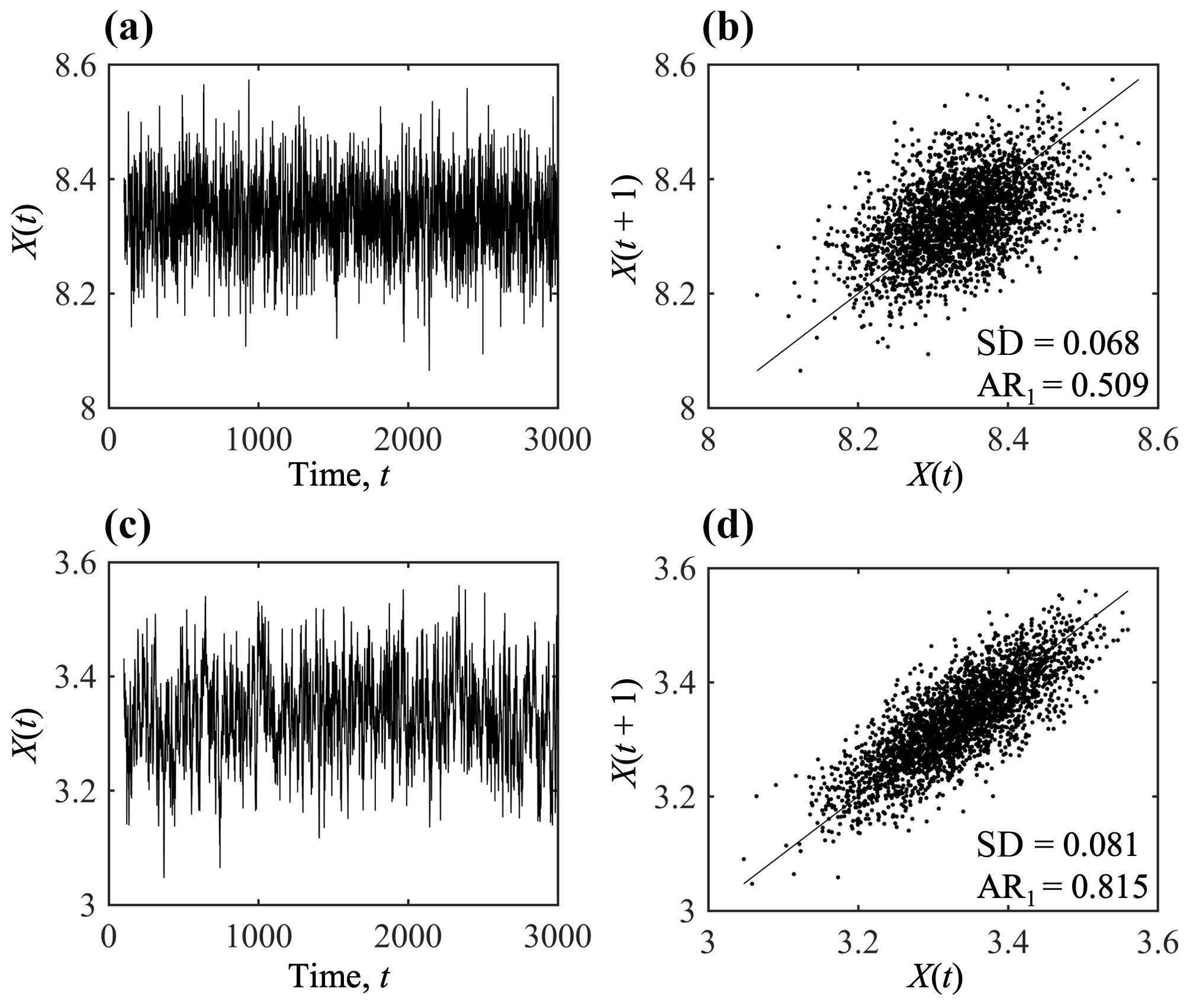
Figure 1 Characteristic changes in the system of a harvested population when approaching the critical transition: (a) population dynamics and (b) statistical metrics when the system is far from tipping (E=0.1); (c) population dynamics and (d) statistical metrics when the system is closer to tipping (E=0.4). Note that the spin-up periods are removed.

2.2.3 Illustrative example of the autocorrelation process

The characteristic changes in the AR₁ and SD in an autocorrelation process are illustrated here using a benchmark example of a harvested population (Beddington and May, 1977). Its governing dynamics are given by a stochastic differential equation:

$$\begin{array}{}\text{(6)}& {\displaystyle \frac{\mathrm{d}X}{\mathrm{d}t}}=\left[r\right(t)-E]X-r_{\mathrm{0}}{X}^{\mathrm{2}}/K.\end{array}$$

Here, $\mathrm{d}X/\mathrm{d}t$ is the net growth rate of population X; $r\left(t\right)=r_{\mathrm{0}}+\mathit{\gamma }\left(t\right)$, where r₀ is the mean value of intrinsic growth rate (set to 0.6 in this example), and γ(t) is a white noise with zero mean; K is the carrying capacity (set to 10); and E is the harvesting rate. Figure 1 shows the evolution of the population subject to the dynamics in Eq. (6) and the results of two statistical metrics with different harvesting rates (0.1 and 0.4 for low and high rates, respectively). When the system is far from the tipping point (low harvesting rate; Fig. 1a and b), its resilience to perturbations is large with a relatively high recovery rate, characterized by a relatively low AR₁ and SD. In comparison, the resilience decreases when the system is closer to the critical transition (high harvesting rate; Fig. 1c and d), and the rate of recovery from perturbations declines as a consequence of critical slowing down. The system has a relatively long memory for perturbations, resulting in a stronger correlation between subsequent states and a larger SD in a stochastic environment (Scheffer et al., 2009).

2.3 Precipitation network analysis

The hydrological system dynamics often evolve on top of complex topological structures such as climate networks (Konapala and Mishra, 2017); their interactions modulate the potential tipping of the system. In this section, we extend the analysis of early-warning signals for precipitation transitions beyond the changes in conventional means (AR₁ and variance) and investigate the system structure represented by the precipitation network of all CONUS cities.

In its simplest form, a network (or graph) can be mathematically represented as a group of nodes or vertices that are connected together. The connection between a pair of nodes is called a link (edge), representing the similarity (or inverse distance) of attributes of the two nodes. Note that we focus here on undirected and unweighted networks only, although the proposed procedure of analysis in this study remains applicable to more complicated (e.g., directed and/or weighted) networks with slight modification.

More specifically, in this study, we treat 481 CONUS cities (see Sect. 2.1) as nodes and construct the network based on monthly precipitation retrieved from the Daymet dataset (Thornton et al., 2018) for the period from 1980 to 2018 (see Sect. 2.1). The connectivity of precipitation networks is constructed using the Pearson correlation coefficient (a commonly adopted distance function) between monthly precipitation time series of two cities i and j (ρ_ij), which is defined as follows:

$$\begin{array}{}\text{(7)}& {\mathit{\rho }}_{ij}={\displaystyle \frac{E\left[\left(P_i-{\mathit{\mu }}_{P_i}\right)\left(P_j-{\mathit{\mu }}_{P_j}\right)\right]}{{\mathit{\sigma }}_{P_i}{\mathit{\sigma }}_{P_j}}},\end{array}$$

where P_i is the precipitation time series, with the subscript i denoting the node (city) number; and μ and σ are the mean and standard deviation of the precipitation time series, respectively. Note that the correlation coefficient is only one kind of measure to describe connectivity, and other similarity (or dissimilarity) functions (e.g., Minkowski distance) (Wang et al., 2020a) are also applicable in network construction. The connectivity between a pair of nodes forms the adjacency matrix A (or A_ij, i, j=1, 2, …, N), which is defined as follows (Tsonis and Roebber, 2004):

$$\begin{array}{}\text{(8)}& {\mathbf{A}}_{ij}=\mathrm{\Theta }\left({\mathit{\rho }}_{ij}-{\mathit{\rho }}_{\mathrm{threshold}}\right),\end{array}$$

where Θ is the Heaviside step function, ρ_threshold is the threshold value, and N is the number of cities. Here, we choose a threshold of 0.5, which is a statistically significant example, as suggested by previous studies (Tsonis and Roebber, 2004; Wang and Wang, 2020).

To investigate the topological feature of the precipitation network and how it evolves over time, four representative metrics are then analyzed: the mean distance (or equivalently the network-average Pearson correlation coefficient), the density, the network modularity, and the clustering coefficient. The mean distance describes the overall connectivity of the network and is given by (Tsonis et al., 2007)

$$\begin{array}{}\text{(9)}& d\left(t\right)={\displaystyle \frac{\mathrm{2}}{N(N-\mathrm{1})}}\sum _{d_{ij}^t\in {\mathbf{D}}^t}{d}_{ij}^t,\end{array}$$

where d(t) denotes the mean network distance at current time t at the center of a sliding window, $d_{ij}^t$ represents the distance between a pair nodes i and j at time t, and D^t is the distance matrix for each sliding window. Equivalently, the mean network distance can be measured using the Pearson correlation coefficient:

$$\begin{array}{}\text{(10)}& d_{ij}^t=\sqrt{\mathrm{2}\left(\mathrm{1}-\mathrm{|}{\mathit{\rho }}_{ij}^t\mathrm{|}\right)}.\end{array}$$

The distance can be thought of as the average correlation between all possible pairs of nodes and is interpreted as a measure of synchronization among different components of a network: a distance of zero corresponds to a complete synchronization (Tsonis et al., 2007). The mean (nodal) Pearson correlation coefficient is

$$\begin{array}{}\text{(11)}& \mathit{\rho }\left(t\right)={\displaystyle \frac{\mathrm{2}}{N(N-\mathrm{1})}}\sum _{{\mathit{\rho }}_{ij}^t\in {\mathbf{D}}^t}{\mathit{\rho }}_{ij}^t,\end{array}$$

and it is clear that the mean distance and the mean Pearson correlation coefficient are inversely correlated when the latter is positive.

The density of a network is the fraction of edges that are present and can have a value between zero and one. It is calculated as follows:

$$\begin{array}{}\text{(12)}& {\mathit{\rho }}^{\prime }={\displaystyle \frac{\mathrm{2}m}{N(N-\mathrm{1})}},\end{array}$$

where m is the total number of edges. The density represents the probability that a pair of nodes picked at random from the whole network are connected by an edge. It plays an important role in the random graph model (Newman, 2018). The larger the density value, the denser the network.

The modularity is the number of edges falling within groups minus the expected number in an equivalent network with edges placed at random. It describes how strong the community structure is (Newman et al., 2006) and is defined as follows:

$$\begin{array}{}\text{(13)}& Q={\displaystyle \frac{\mathrm{1}}{\mathrm{2}m}}\sum _{ij}\left(A_{ij}-{\displaystyle \frac{k_i{k}_j}{\mathrm{2}m}}\right){\mathit{\delta }}_{g_i{g}_j},\end{array}$$

where g_i is the group to which node i belongs, δ_ij is the Kronecker delta function, and k_i is the degree (number of links) of node i. A network with positive and large modularity values is preferable for research and real-world applications (Newman and Girvan, 2004).

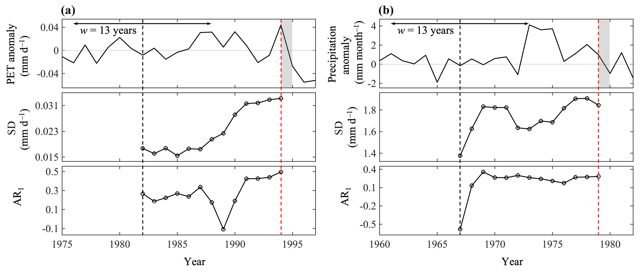
Figure 2 Time series of anomalies, AR₁, and SD of global (a) PET and (b) precipitation. The horizontal lines with arrows show the width of one moving window (13 years), the vertical dashed red lines represent critical transitions, and the gray bands represent the transition phase.

The clustering coefficient of a network is defined as follows:

$$\begin{array}{}\text{(14)}& C={\displaystyle \frac{\mathrm{1}}{N}}\sum _{i=\mathrm{1}}^N{\displaystyle \frac{n_i}{k_i\left(k_i-\mathrm{1}\right)/\mathrm{2}}},\end{array}$$

where n_i is the number of edges among the nearest neighbors of the ith node. Topologically, the clustering coefficient is the fraction of paths with the length equal to two in the network that are closed, and it quantifies the extent to which a pair of nodes with common neighbor are also neighbors of each other (Newman, 2018).

3 Results and discussion

3.1 Statistical measures of early-warning signals

We first identify the conventional early-warning signals at the global scale, the AR₁ and SD, for the potential evapotranspiration and precipitation anomalies using the algorithm detailed in Sect. 2.2. Figure 2 shows PET and precipitation anomalies and the early-warning signals prior to critical transitions. The critical transition of global PET occurred in the year 1994 (denoted by the red dashed line in Fig. 2a), which is generally consistent with the transition of the solar radiation trend at the Earth's surface in ∼1990 (Pinker et al., 2005; Wild et al., 2005). This transition from decreasing to increasing global radiation (also known as the transition from global dimming to brightening) has been found in many observational records, primarily due to changes in cloudiness, aerosol loadings, and atmospheric transparency (Pinker et al., 2005). It is clear from Fig. 2a that both the AR₁ and SD of global PET increased gradually over time for more than 1 decade (one sliding window) prior to the critical transition. Per theoretical analysis in Sect. 2, the increase in the AR₁ and SD apparently presages the critical slowing down of the rate of recovery from perturbation, as the system evolved approaching the transition in 1994.

We then proceed to identify early-warning signals for precipitation at the city scale, following the same procedure as that utilized for the global-scale analysis above. Figure 3 shows the results for four CONUS cities (New York City, NY; Seattle, WA; Fresno, CA; and Miami, FL). These cities were preselected as being representative of the distinct regional geographic conditions and background climates of their locations. Note that the monthly precipitation data are from 1895 to 2019 (125 years) for New York City and Fresno, whereas the data are from 1948 to 2019 (72 years) for Seattle and Miami. For individual cities, the times (years) at which the critical transition occurred in the precipitation records differ: 1967 for New York City, 1993 for Seattle, 1971 for Fresno, and 1993 for Miami. The results are generally in good agreement with studies on climate phase changes. Those phase changes have been associated with significant changes in climate variability, such as global temperature, ENSO, and the IPO. For example, the switch of the IPO from a cold phase to a warm phase around 1977 induced a clear upward trend in precipitation over much of the western and central regions (e.g., Oklahoma, Kansas, and Missouri) of the CONUS, whereas a latter shift in around 1999 (back to a cold phase) resulted in decreased precipitation (Dai, 2013). The results of early-warning signals are also shown in Fig. 3. Here, again, we find that the statistical measures of the AR₁ and SD generally increase with time in all four cities prior to the emergence of transitions.

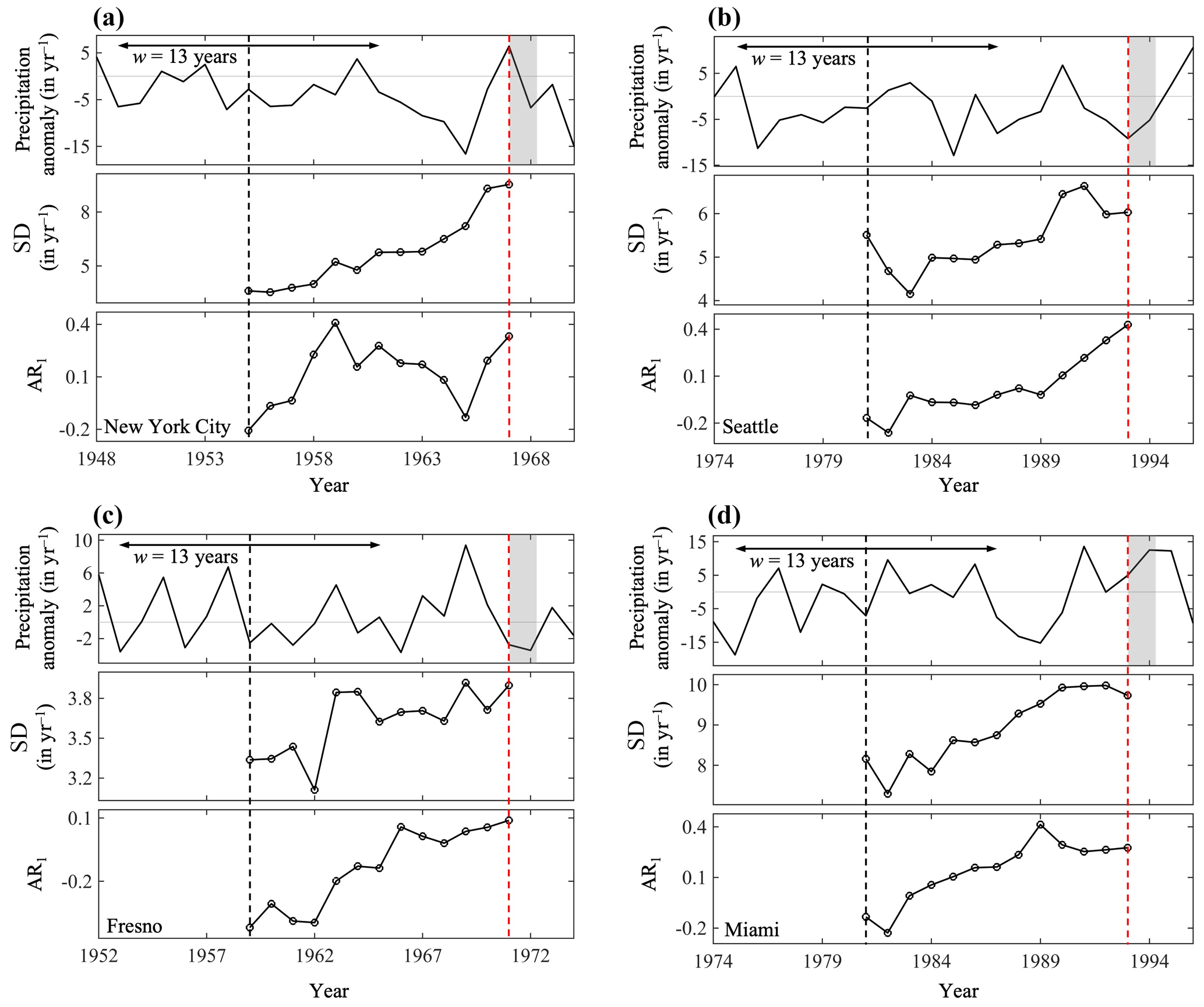
Figure 3 Time series of anomalies, AR₁, and SD of precipitation in (a) New York, (b) Seattle, (c) Fresno, and (d) Miami in the CONUS. The horizontal lines with arrows show the width of one moving window (13 years), the vertical dashed red lines represent critical transitions, and the gray bands represent the transition phase.

Table 1 The division of CONUS cities into nine geographical regions.

3.2 Network representation of critical transitions

In this section, we extend the concept of early-warning signals for critical transitions in hydrological systems from conventional time series analysis to the topological analysis of their network structure. We first construct the precipitation networks based on the monthly precipitation data for all CONUS 481 cities in the period from 1980 to 2018 retrieved from the Daymet dataset (Thornton et al., 2018), with a threshold similarity of 0.5 (detailed in Sect. 2.3). The CONUS precipitation network generated using the entire time series (39 years × 12 months) is shown in Fig. 4a. All CONUS cities are further subdivided into nine geographic regions following Wang and Wang (2020), as listed in Table 1. The connectivity, represented by the adjacency matrix, of the precipitation network is shown in Fig. 4b, with the nine regions marked.

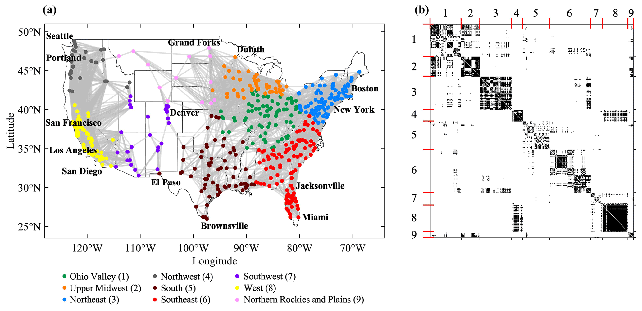
Figure 4 The precipitation network of CONUS cities: (a) the geographic map of connectivity and (b) the adjacency matrix, with A_ij=1 in black (connected), A_ij=0 in white, and the short red lines marking the divisions of the nine geographic regions in accordance with panel (a).

From Fig. 4, it is clear that the 39-year aggregated CONUS urban precipitation network is largely occupied by intra-regional connection, manifest as regional clusters on the geographic map (Fig. 4a) and dark (connected) diagonal blocks in the adjacency matrix (Fig. 4b). This is consistent with a clustering analysis based on monthly precipitation (1981–2010) in CONUS cities (Wang et al., 2020a). This is physical, as the patterns of precipitation and its anomalies in a city are predominated by the geographic controls and background climate conditions in the region where the city is located. Thus, the dense intra-regional connections (diagonal blocks in Fig. 4b) reveal the similarity of precipitation patterns among cities with a similar climate environment, or, in other words, “like is connected to like” (Newman and Girvan, 2004). This topological feature also shows that the CONUS precipitation network is highly assortative with large modularity (Q=0.589), as the modularity reveals network community structures.

In addition to the modular structure reflected as dense intra-regional connectivity, the precipitation network also includes some inter-regional (Fig. 4a) or “off-diagonal” (Fig. 4b) connections. The presence of long-range, out-of-region connectivity is usually formed by complex interactions via atmospheric gateways (teleconnection) (Boers et al., 2019). For example, it is found that precipitation patterns are similar in the Ohio Valley (Region 1) and Upper Midwest (Region 2) (same for the West and Northwest), which is shown as the off-diagonal connection in Fig. 4b. Similar hydrological teleconnections have been observed in Konapala and Mishra (2017) and Wang et al. (2020a). For example, Konapala and Mishra (2017) found that the Ohio Valley region plays an important role in propagating droughts (with higher values of outward strength) toward adjacent regions such as the Upper Midwest (Region 2) and Northeast (Region 3), consistent with the off-diagonal connections shown in Fig. 4b.

To find how the network structure responds to (or presages, as early-warning signals of AR₁ and SD) critical transitions in the CONUS precipitation system, we then proceed to construct the time-varying networks (cf. the aggregated 39-year network in Fig. 4) using a sliding window of 7 years (following Sect. 2.2) from the same 39-year (1980–2019) set of Daymet precipitation data. In addition, we follow the same procedure for analyzing the time series of cumulative precipitation in the CONUS and determine the year of critical transition at the emergence of abrupt change in the slope of cumulative precipitation. In this case, the critical transition for precipitation in the CONUS urban areas was around the year 1998, which is consistent with the IPO phase changes in the 1990s (Dai, 2013; Deser et al., 2004). This can also be seen from Fig. 5a, as the early-warning signal of SD had a clear increasing trend, whereas the trend of AR₁ was slightly obscure with a 7-year window size. Nevertheless, a clear increase immediately prior to the transition is still observed for the AR₁ in Fig. 5a.

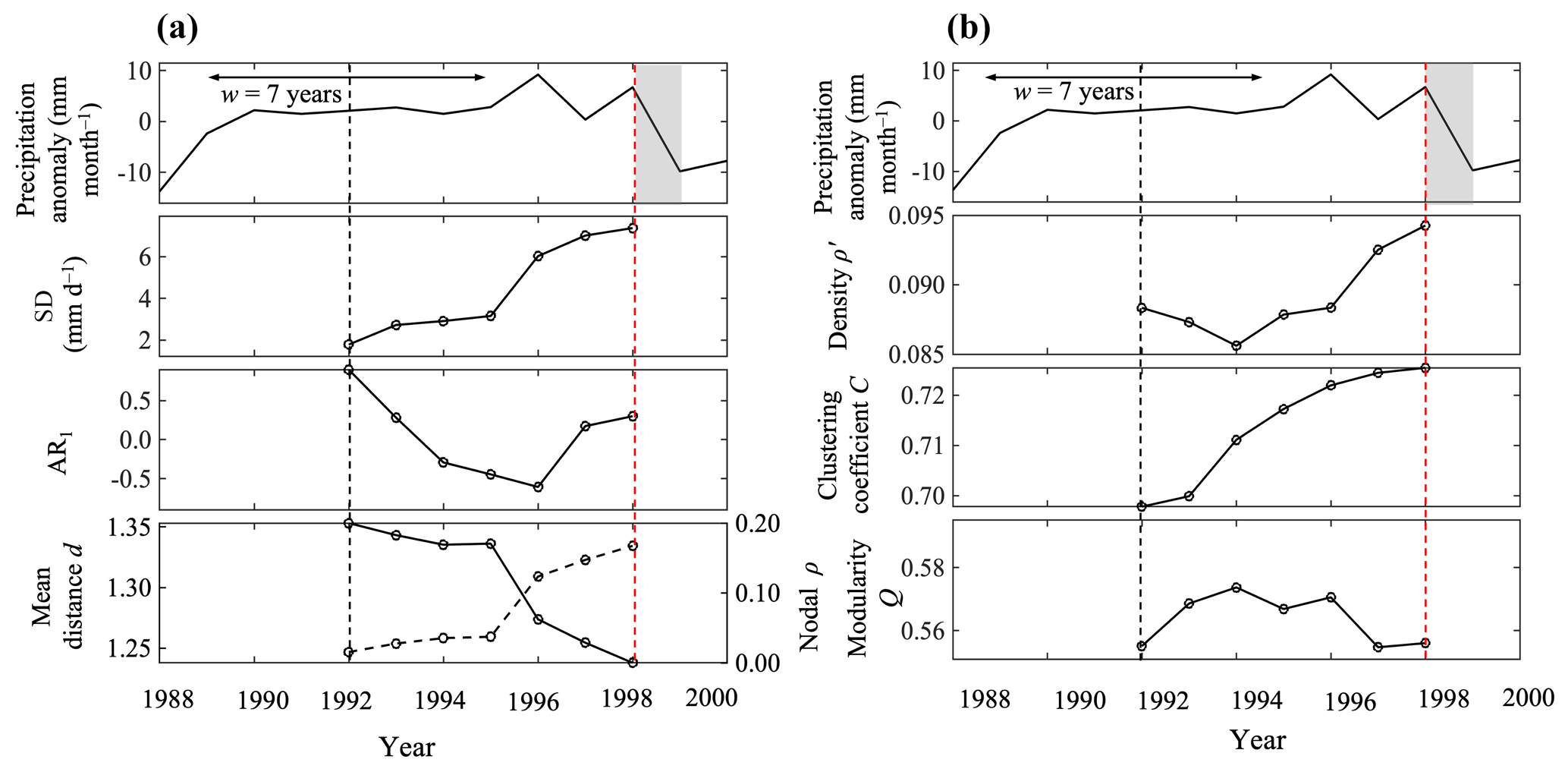
Figure 5 Early-warning signals and structural responses to the critical transitions (in the year 1998) in time-varying CONUS precipitation, as the time evolutions of (a) precipitation anomalies, AR₁, SD, and the mean distance (d) and similarity (ρ) functions for network construction, and (b) network topological parameters of clustering coefficient (C), density (ρ^′), and modularity (Q). The horizontal lines with arrows show the width of one moving window (7 years), the vertical dashed red lines represent critical transitions, and the gray bands represent the transition phase.

In addition, we also find that the network topology has a significant response to the critical transition, as shown in Fig. 5. The mean nodal correlation coefficient ρ, the network density ρ^′, and the clustering coefficient C all exhibited a clear trend of increase prior to the transition. Note that ρ is the structural parameter prior to the construction of networks, whereas ρ^′ and C are posterior parameters determined from the topology of constructed networks. Furthermore, the mean distance d is (nearly) inversely correlated with the mean nodal correlation coefficient, so it is expected that d decreased prior to the transition. The increase in ρ (or, equivalently, the decrease in d) suggests that, on average, the connectivity among all cities in the CONUS precipitation network was enhanced prior to the transition. This is likely attributable to the strengthening of synchronization of precipitation events (Boers et al., 2016; Rheinwalt et al., 2016) via, e.g., propagation of precipitation fronts entraining larger urban areas than before, as a result of critical slowing down in recovery from system perturbation (e.g., extreme rainfalls). Similar patterns of increases in structural correlation ρ and decreases in mean distance have been observed in other climate networks by Tsonis et al. (2007).

The enhanced network connectivity prior to critical transitions, manifested as an increase in nodal correlation ρ (or a decrease in mean distance d), led to the increase in the total number of links and the network density ρ^′ (the fraction of edges in the network) (Fig. 5b). The clustering coefficient C also increased as a result of enhanced community structure predominated by the intra-regional connections (Fig. 4). In contrast, the modular structure of the precipitation network remained insusceptible to the emergence of critical transition and enhanced synchronization of precipitation events, with the value of modularity Q fluctuating around 0.55–0.57 in the 7-year window size. This is seemingly because the critical transition tends to enhance both the local community structure (intra-regional connection) and the teleconnection (inter-regional connection), thereby leaving the modular organization of the entire network unchanged. Qualitatively, this means that the topological structure of the CONUS precipitation network, despite its temporal evolution and changes in the overlying dynamics (the occurrence of critical transition or slowing down), remains “like is connected to like”.

4 Concluding remarks

In this study, we investigated the early-warning signals of potential critical transitions in the hydrological system, in particular the precipitation and PET, as a result of the critical slowing down of system recovery rate from dynamic perturbation. The occurrence of critical transitions in precipitation climatology agreed with recorded observation, consistent with climate shifts in the 1970s and 1990s due to low-frequency variability such as SST or IPO. The theoretical basis of their early-warning signals, statistically measured in terms of the AR₁ and SD (variance), was illustrated using an autocorrelation process and a harvested population model. We applied the analysis to the long-term global-scale precipitation and PET time series as well as a city-scale precipitation dataset in the CONUS. It was found that the emergence of increasing trends in the AR₁ and SD, prior to critical transitions in all cases, agrees well with theoretical predictions.

In addition, we extended the conventional statistical measures of early-warning signals to system-based network analysis. We constructed precipitation networks over all urban areas in the CONUS and calculated some key topological parameters including the mean similarity/distance function, network density, clustering coefficient, and modularity. The system evolution toward the critical transition apparently enhances the synchronization of precipitation events over CONUS urban areas, leading to the strengthening of the community structure as well as teleconnections in the network. As a result, we identified the increasing trends of the mean network correlation, the density, and the clustering coefficients due to system transitions; therefore, these structural parameters can be used as network-based precipitation system early-warning signals, similar to the process-based measures of the AR₁ and variance. The network modularity, on the other hand, is not susceptible to and cannot be interpreted as a harbinger of critical transitions in the precipitation system. These findings help to shed new light on the intricate structure–dynamic interactions in complex climate systems that modulate the future trend of the evolution of hydrological processes under global climate change.